
 ?Mathematical formulae have been encoded as MathML and are displayed in this HTML version using MathJax in order to improve their display. Uncheck the box to turn MathJax off. This feature requires Javascript. Click on a formula to zoom.
ABSTRACT
In this paper, we focus on multivariate doubly truncated first two moments of generalized skew-elliptical distributions. This class of distributions includes many useful distributions, such as skew-normal, skew Student-, skew-logistic and skew-Laplace-normal distributions, as special cases. The formulas of multivariate doubly truncated covariance (MDTCov) for generalized skew-elliptical distributions are also given. Further, we compute multivariate doubly truncated expectations (MDTEs) and MDTCovs for
-variate skew-normal, skew-Student-
, skew-logistic and skew-Laplace-normal distributions, and use Monte-Carlo method to simulate and compare with the above results. As applications, the results of multivariate tail conditional expectation (MTCE) and multivariate tail covariance (MTCov) for generalized skew-elliptical distributions are derived. In addition, an optimal problem involving MDTE and MDTCov risk measures is proposed. Finally, we use real data to fit skew-normal distribution and to discuss MTCEs and MTCovs of logarithm of adjusted prices for two portfolios consisting of three companies from S&P (Standard & Poor’s) sectors.
1. Introduction
Truncated moments’ expansions are applied to many fields including the design of experiment (Thompson Citation1976), robust estimation (Cuesta-Albertos et al. Citation2008), outlier detections (Riani et al. Citation2009; Cerioli Citation2010), robust regression (Torti et al. Citation2012), robust detection (Cerioli et al. Citation2014), statistical estates’ estimation (Shi et al. Citation2014), risk averse selection (Hanasusanto et al. Citation2015), and entropy computation and application (Milev et al. Citation2012; Zellinger and Moser Citation2021). Therefore, the related research of truncated moment is developed to different distributions by many scholars.
Since (Tallis Citation1961) has given an explicit formula for the first two moments of a lower truncated multivariate standard normal distribution by moment generating function, (Amemiya Citation1974 and Lee Citation1979) used results (Tallis Citation1961) for extending (Tobin Citation1958)‘s model to the multivariate regression and simultaneous equations models when the dependent variables are truncated normal. Lien (Citation1985) provided the expressions for the moments of lower truncated bivariate log-normal distributions. Kim (Citation2008) studied the moments of a doubly truncated generalized Student- distribution and its utility for solving statistical problems. Manjunath and Wilhelm (Citation2012) computed the first and second moments for the rectangularly double-truncated multivariate normal density, and extended the derivation of Tallis to general
,
and for double truncation. Arismendi (Citation2013) derived formulae for the higher order tail moments of the lower truncated multivariate standard normal, Student-
, lognormal and a finite-mixture of multivariate normal distributions. Arismendi and Broda (Citation2017) deeply derived multivariate elliptical lower truncated moment generating function, and first second-order moments of quadratic forms of the multivariate normal, Student-
and generalized hyperbolic distributions. Moreover, Ho et al. (Citation2012) presented general formulae for computing the first two moments of the truncated multivariate Student-
distribution under the double truncation. Recently, Kan and Robotti (Citation2017) provided expressions of the moments for folded and doubly truncated multivariate normal distribution. Galarza et al. (Citation2021) and Morales et al. (Citation2022) generalized moments of folded and double truncated to multivariate Student-
and extended skew-normal distributions, respectively. Also, Ogasawara (Citation2021b) presented unified and non-recursive formulas for moments of the normal distribution with stripe truncation. Ogasawara (Citation2021a) further derived a non-recursive formula for various moments of the multivariate normal distribution with sectional truncation, and introduced the importance of truncated moments in biological field, such as animals or plants breeding programmes (Herrendörfer and Tuchscherer Citation1996) and medical treatments with risk variables as blood pressures and pulses, where low and high values of the variables are of primary concern. Valeriano et al. (Citation2021) investigated moments and random number generation for the truncated elliptical family of distributions. Galarza et al. (Citation2022) further computed doubly truncated moments for the selection elliptical class of distributions, and established sufficient and necessary conditions for the existence of these truncated moments.
From a practical viewpoint, skewed distribution model is more useful than non-skewed distribution model because of data sets possessing large skewness and/or kurtosis measures (for instant, in economic and financial data sets). Based on this reason, many skew distributions and their some properties were researched, including skew normal (Azzalini and Capitanio Citation1999), skew- (Azzalini and Capitanio Citation2003), mixture of skew-normal (Mousavi et al. Citation2019), mixture of elliptical (Zuo and Yin Citation2021), generalized skew normal (Huang et al. Citation2013), generalized skew-elliptical (Genton Citation2004), generalized skew two-piece skew-normal (Jamalizadeh et al. Citation2011) and generalized skew two-piece skew-elliptical (Salehi et al. Citation2014) distributions and so on. Also, Roozegar et al. (Citation2020) derived explicit expressions of the first two moments for doubly truncated multivariate normal mean-variance mixture distributions.
Firstly, since the real data set is not symmetric or has a heavy tail, the symmetric distribution does not fit to it well (see Eini and Khaloozadeh Citation2021). Secondly, the majority of researches has been done to calculate the doubly (or lower) truncated moments to symmetric (elliptical) distribution but less attention has been paid to asymmetric distribution. Thirdly, the (doubly) truncated moments can be applied to many fields, especially, in economics and finance (computing measures of risk or portfolio risk). Finally, due to the great flexibility of the skewing function and the extent of the elliptical family, the generalized skew-elliptical (GSE) distributions family include many commonly used skewed and symmetric distributions. This family of distributions not only facilitates the modelling of skewness but also adeptly captures heavy tails. Interesting special cases are discussed in Fang et al. (Citation1990); Fang and Zhang (Citation1990); Azzalini and Capitanio (Citation1999); Branco and Dey (Citation2001); Genton (Citation2004). Based on the above reasons, we derive multivariate doubly truncated first two moments for GSE distributions and provide expressions of multivariate doubly truncated expectation and covariance for this class of distributions. Some important cases of those distributions, including skew-normal (SN), skew Student- (SSt), skew-logistic (SLo) and skew-Laplace-normal (SLaN) distributions, are also presented. As applications, formulas of MTCE and MTCov for GSE distributions are derived by our results established. Furthermore, an optimal problem involving MDTE and MDTCov risk measures is proposed and its solution is given.
The remainder of the paper proceeds as follows. In Section 2, we introduce preliminaries, including the GSE distributions and notation. Section 3 focuses on multivariate doubly truncated moments for GSE distributions, deriving formulas for their multivariate doubly truncated first two moments. In Section 4, we show some special cases. As applications, MTCE and MTCov risk measures for GSE, and an optimal problem involving MDTE and MDTCov risk measures are given in Section 5. Numerical illustrations are shown in Section 6. Specifically, this section compares MDTE and MDTCov of the several distributions, presents a comparison between simulated estimation and formula calculation, and also discusses MTE and MTCov of logarithm of adjusted prices for six companies. Finally, the paper closes with the concluding remarks.
2. Preliminaries
We start with the definition of GSE distributions as follows.
2.1. Generalized skew-elliptical distributions
Class of generalized skew-elliptical distributions was introduced by Genton (Citation2004) and has been widely discussed in many literatures (e.g. Genton and Loperfido (Citation2005); Shushi (Citation2016); Adcock et al. (Citation2021)). A random vector
is said to have a generalized skew-elliptical distribution if its probability density distribution (pdf) exists and has the form
where
is the pdf of a -dimensional elliptical random vector with location vector
, scale matrix
and density generator
,
(see, for instance, Landsman and Valdez (Citation2003)). Here
is normalizing constant. The density generator satisfies
Here is the skewing function, which satisfies
and
for
. From
, we can define skewing function
through
for
and
. If
is a
-dimensional generalized skew-elliptical random vector with pdf
, the random vector
(
means ‘equally distributed’) will follow a doubly truncated multivariate distribution with pdf given by
where ,
,
and
, i.e.
, for
,
denoted by
and
is the indicator function.
We define cumulative generators and
as follows (see Landsman et al. (Citation2018)):
and
and their normalizing constants are, respectively, written as (see Zuo et al. (Citation2021)):
and
For those density generators, it is necessary to meet the following conditions
and
Now, we define elliptical random vectors and
. Their form of pdf (if them exist) are as follows, respectively:
Let and
be the corresponding generalized skew-elliptical random vectors.
Next, we introduce some notations.
Notation
Assume is an arbitrary random vector with probability density function
, for any fixed
, writing
and
Denoting
and
To give an expression for the multivariate doubly truncated moment, we denote the doubly truncated expectation of
-dimensional random vector
with pdf
as
where is a function.
Remark 1. When = 1, doubly truncated expectation will be denoted by
; When
, the doubly truncated expectation will be tail expectation:
which is defined by Zuo and Yin (Citation2022a).
The following notation will be used throughout this paper: ,
and
denote the cumulative distribution functions (cdf) of the univariate standard normal, Student-
(with degrees of freedom
) and logistic distributions;
,
and
denote the pdfs of the univariate standard normal, Student-
(with degrees of freedom
) and logistic distributions, respectively.
3. Multivariate doubly truncated moments
Let be a random vector with finite fixed vector
, positive defined fixed matrix
and pdf
. Let
Writing
.
Now, we define ,
and
, the pdfs associated with elliptical random vectors
,
and
, respectively:
where
,
and
. In addition,
,
and
are corresponding normalizing constants of
,
and
, which are written as:
and
Next, we present explicit expressions for the multivariate doubly truncated (first two) moments of generalized skew-elliptical distributions.
Theorem 1.
Let
be as in (1). Suppose that
satisfies conditions (3), (5) and (6). Further, assume
and
exist for
. Then
where is a
symmetric matrix, and
is a
vector. Here
,
,
,
, and pdfs of
,
and
are same as in (7), (8) and (9), respectively. The corresponding normalizing constants
,
and
are as in (10), (11) and (12), respectively. In addition,
and
.
See the Appendix.
Zuo et al. (Citation2023) proposed multivariate range Value-at-Risk (MRVaR) and covariance (MRCov) risk measures for a random vector
:
where The above two risk measures are applicable in finance and risk management. Furthermore, they pointed out that regulatory constrains, investment target and risk management requirement (e.g. credit rating level) can be considered in determining desirable
and
.
As their generalization, we define MDTE and MDTCov for a random vector
as follows, respectively:
and
Now, we can give following result of MDTE and MDTCov for GSE distributions.
Proposition 1.
Under the conditions of Theorem 1, we have
where and
are the same as those in Theorem 1.
See the Appendix.
The MDTE and MDTCov for a random vector
include multivariate upper expectation (MUE) and Covariance (MUCov), respectively:
and
In Landsman et al. (Citation2018), authors derived multivariate tailed Chebyshev-type inequality. For the MUE and MUCov, we have multivariate upper Chebyshev-type inequality as follows.
Proposition 2.
For any and
random vector
, we have the following inequality:
See the Appendix.
4. Special cases
This section focuses ,
and
for important special cases of the GSE distributions, including SN, SSt, SLo and SLaN distributions. Their forms of
,
and
are given in (13), (14) and (18), respectively, so that we merely present
,
,
and
.
Corollary 1
(SN distribution). Let . The pdf of
is
In this case, ,
and
where
. Since
denotes the pdf of
(the
-variate normal distribution with mean vector
and covariance matrix
). So
and
. Thus,
,
,
and
.
Corollary 2
(SSt distribution). Let . Here
is degrees of freedom and
. The pdf of
is
In this case,
and
with . So
and
can be expressed, respectively, as
and
In addition,
and
where and
denote Gamma function and Beta function, respectively. Since
and
so that
and
Then
,
,
,
,
,
,
,
,
and
.
Therefore, ,
and
can be further simplified as
and
Corollary 3
(SLo distribution). Let , where
. The pdf of
is
In this case,
and .
denotes generalized Hurwitz-Lerch zeta function (see, for instance, Lin et al. (Citation2006)).
and
are expressed as
In addition,
Since
and
so that
and
Then
,
,
,
and
.
Therefore,
and
Corollary 4
(SLaN distribution). Let , where
. The pdf of
is
In this case, and
So
In addition,
Since
and
thus
and
Then
,
,
,
and
.
,
and
can be further simplified as
and
5. Applications
In this section, we mainly consider MTCE and MTCov for GSE distributions. Furthermore, we apply MDTE and MDTCov risk measures to construct an optimal problem.
Landsman et al. (Citation2018) proposed a new MTCE for a vector of risks
with cdf
:
where
and ,
, denotes the
-th quantile of
. See Landsman et al. (Citation2016) for a special case when
Landsman et al. (Citation2018) further proposed a novel form of MTCov:
From Proposition 1, we give the following corollary.
Corollary 5
Let
be as in (1). Suppose that it satisfies conditions
and
Further, assume and
exist for
. Then
where is a
symmetric matrix, and
is a
vector. Here
,
,
,
,
,
and
are given in Theorem 1. In addition,
is the tail function of
.
Proof.
Letting and
in Theorem 1 and Proposition 1, and combining with conditions (22) and (23), we can instantly obtain above results, ending the proofs.
Note that the results and
of Corollary 5 coincide with Theorem 3.1 and Theorem 1 in Zuo and Yin (Citation2022b, Citation2022a), respectively.
Example 1
(SN distribution). Let . Then, forms of MTCE and MTCov of
are the same as in (24) and (25), and
and
are given by
where
,
,
and
are given in Corollary 1.
Let be an
risk assets,
be expected returns, and
be covariance matrix of
. For our portfolio
, there is following optimal problem:
which satisfies condition and
, where
,
, and
is a risk-free rate.
Suppose that we have a system of risks of assets such that
. The above classical optimal model can extend to following optimal problem involving MDTE and MDTCov risk measures of
. That is to say, we suggest taking the MDTE and MDTCov measures instead of the expectation and covariance matrix of the portfolio risk, i.e.
We would have following an optimal problem:
which satisfies condition .
For above optimal problem, there is following theorem.
Theorem 2.
Assume is invertible, the optimal solution of (27) subject to
, is given by
The proof relies on the classical optimal solution of (26) if
and
substitute with
and
.
6. Numerical illustrations
In this section, we compare MDTEs and MDTCovs for the skew-normal (SN), skew-Student- (SSt), skew-logistic (SLo) and skew-Laplace-normal (SLaN) distributions, examine MDTE, MDTCov for the skew-normal (SN) distribution, and discuss MTCE and MTCov of logarithm of adjusted prices for six companies.
A comparison of MDTE and MDTCov for several skewed distributions
Firstly, we compute and compare MDTEs and MDTCovs for the SN, SSt, SLo and SLaN distributions. Let , and denote
,
,
and
with parameters
By Theorem 1, Proposition 1 and Corollaries 1-4, we can obtain MDTEs and MDTCovs for ,
,
and
in
, as follows:
The MDTEs of ,
,
and
for
are pictured in .
Figure 1. of
,
,
and
for
.
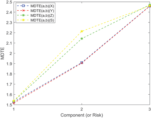
For MDTEs, from we find that the MDTE of skew-Student- distribution is least among the four at
, and skew-Laplace-normal distribution is almost largest among the four at
except for component (or risk) 3. Moreover, the MDTE of the skew-Student-
and skew-normal models distinguishes little from each other. As for MDTCovs, we observe that the diagonal of
matrix under skew-logistic distribution is almost largest among the four at
except for component (or risk) 2, and the diagonal of
matrix under skew-normal is almost largest among all models at
except for component (or risk) 3.
6.2. A comparison between simulated estimation and formula calculation
Now, to compare our approach and Monte Carlo method, without loss of generality (or for the sake of simplicity), we use -dimensional skew-normal, skew-Student-
, skew-logistic and skew-Laplace-normal distributions as examples. We compute multivariate doubly truncated expectation, multivariate doubly truncated covariance for SN, SSt, SLo and SLaN distributions. Let
,
,
,
and
with parameters
From Theorem 1, Proposition 1 and Corollaries 1-4, the multivariate doubly truncated expectation and multivariate doubly truncated covariance matrix of ,
,
and
for
can be obtained as
We use Monte-Carlo method (R software) to simulate them as presented in :
Figure 2. The trace plots of the Monte Carlo estimates of the elements of μ
(
(left) and
(right)).
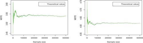
Figure 3. The trace plots of the Monte Carlo estimates of the three elements of Σ (
(left),
(center) and
(right)).
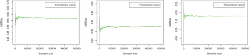
Figure 4. The trace plots of the Monte Carlo estimates of the elements of μ
(
(left) and
(right)).
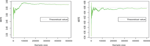
Figure 5. The trace plots of the Monte Carlo estimates of the three elements of (
(left),
(center) and
(right)).
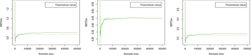
Figure 6. The trace plots of the Monte Carlo estimates of the elements of μ
(
(left) and
(right)).
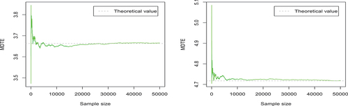
Figure 7. The trace plots of the Monte Carlo estimates of the three elements of Σ (
(left),
(center) and
(right)).
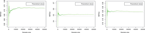
Figure 8. The trace plots of the Monte Carlo estimates of the elements of μ
(
(left) and
(right)).
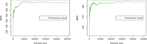
Figure 9. The trace plots of the Monte Carlo estimates of the three elements of Σ (
(left),
(center) and
(right)).
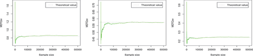
The trace plots in , respectively, display the evolution of Monte-Carlo estimates of the elements of and
, for growing sample sizes. Here, the dotted line represents the corresponding theoretical value. As we see in , with the increase of the number of samples, the MDTE or MDTCov value estimated by Monte Carlo becomes more stable and closer to the theoretical value (as we expect). Furthermore, we observe that the number of samples need to be large enough in order to get the parameter value estimated by Monte Carlo method closer to the theoretical value.
The trace plots in , respectively, display the evolution of Monte Carlo estimates of the elements of and
, for growing sample sizes. The trace plots in , respectively, display the evolution of Monte Carlo estimates of the elements of
and
, for growing sample sizes. The trace plots in , respectively, display the evolution of Monte Carlo estimates of the elements of
and
, for growing sample sizes. Here the dotted line represents the corresponding theoretical value. From , we find that for theoretical value and estimated value by Monte Carlo method, (skewed normal distribution), (skewed Student-t distribution), (skewed logistic distribution) and (skewed Laplace-normal distribution) have similar conclusions.
6.3. Real data analysis
Next, we discuss the logarithm of adjusted prices of two portfolios consisting of three companies from SP (Standard
Poor’s) sectors. Financials sector (the first portfolio) includes Chubb Limited, Cincinnati Financial and Citigroup Inc. companies, and Energy sector (the second portfolio) includes ConocoPhillips, Devon Energy and Chevron Corp. companies (see Amiri and Balakrishnan (Citation2022) for details). The data are from the workdays for the period 1 April 2020 to 31 March 2021.
Because parameter evaluation of GSE distributions is still an unresolved and complex issue (or problem). At present, we find that R Package has a selection function for different subfamilies through their Akaike information criteria (AIC) and Bayesian information criteria (BIC). The subfamilies of this package include the multivariate scale mixtures of normal (SMN), the multivariate scale mixtures of skew-normal (SMSN) and the multivariate skew scale mixtures of normal (SSMN) classes.
Let and
, where
and
are, respectively, the logarithm of opening prices of the
th company in the Financials and Energy sectors. Then, we use the
package to choose the model in each subclass, and their AIC and BIC values are shown in .
Table 1. Fitted distributions and their information criterion values to the logarithm of adjusted prices of different sectors.
The skew-normal distribution has the minimum AIC and BIC among others for and
. Thus, we consider the skew-normal distribution for the observations as
and
. Parameters are estimated by maximum likelihood method:
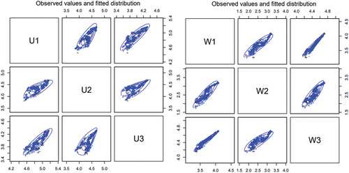
PP-plots and bivariate scatter plots, with contour lines, for the skew-normal distributions are shown in .
Figure 10. PP plot for the skew-normal distribution for the logarithm of adjusted prices of companies in the financials (left) and energy sectors (right).
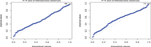
Figure 11. Bivariate scatter plots with contour lines for the skew-normal distribution for the logarithm of adjusted prices of companies in the financials (left) and energy sectors (right).
Let , from Example 1 and Corollary 5, VaRs and MTCEs of
and
for
are presented in , respectively. Specifically,
and
can be computed by EquationEquation (20)
(20)
(20) . As for
and
, we can calculate corresponding
,
and
by Example 1, then we can obtain
and
by EquationEquation (24)
(24)
(24) .
Table 2. The VaRs of and
for
.
Table 3. The MTCEs of and
for
.
As we see in , there is a clear difference between the and
. For
, the value of MTCE of Risk
(first component) is greatest, and the value of MTCE of Risk
(second component) is least. That is to say, for Financials sector, value of MTCE of Chubb Limited company is greatest, and value of MTCE of Cincinnati Financial company is least. However, for
, the value of MTCE of Risk
(third component) is greatest, and the value of MTCE of Risk
(second component) is least. It means that for Energy sector, value of MTCE of Chevron Corp. company is greatest, and value of MTCE of Devon Energy company is least. On the principle that the larger MTCE will have the better return, for Financials sector, we may prefer Chubb Limited company; For Energy sector, we may prefer Chevron Corp. company.
Then, MTCovs of and
for
are presented as follows:
and
From MTCov of (diagonal elements), we observe that value of MTCov of
is greater than the others, and value of MTCov of
is least than the others. It indicates that for Financials sector, value of MTCov of Chubb Limited company is greater than the others, and value of MTCov of Cincinnati Financial company is least than the others. However, there is a big difference between
and
. As we can see, value of MTCov of
is greater than the others, and value of MTCov of
is least than the others. It signifies that for Energy sector, the value of MTCov of Devon Energy company is greater than the others, and value of MTCov of Chevron Corp. company is least than the others. On the principle that the smaller MTCov will have the smaller the risk, for Financials sector, we may prefer Cincinnati Financial company; For Energy sector sector, we may prefer Chevron Corp. company.
By Proposition 2 of Landsman et al. (Citation2018), for and
, we can construct two confidence ellipsoids with probability
:
and
For example, we find that , but
. This indicates that
belongs to the
-tail confidence ellipsoid of
, while it is outside of
-dimensional ellipsoid of
.
7. Concluding remarks
In this paper, we have studied multivariate doubly truncated first two moments of GSE distributions, which provide further generalization of the moments for the doubly truncated multivariate normal mean-variance mixture distributions (Roozegar et al. (Citation2020)). With more emphasis on several important cases, for examples, SN, SSt, SLo and SLaN distributions. We have also presented MDTE and MDTCov for GSE distributions providing further generalization of the MDTE and MDTCov for elliptical distributions. As applications of our results, the MTCE and MTCov for generalized skew-elliptical distributions and an optimal problem involving MDTE and MDTCov risk measures are given. Aim to examine established results, we have used Monte Carlo method to estimate parameters. Kollo (Citation2008) have introduced skewness and kurtosis characteristics of a multivariate -dimensional distribution, and derived expressions for the measures of skewness and kurtosis for the multivariate Laplace distribution. Loperfido (Citation2020) have investigated some properties of Koziol’s measures of multivariate kurtosis. It will, of course, be of interest to introduce and research doubly truncated skewness and kurtosis characteristics of a multivariate distribution, and present expressions of multivariate doubly truncated skewness and kurtosis for GSE distributions in a future paper.
CRediT authorship contribution statement
B. Zuo: Investigation, Writing, Software. S. Wang: Software. C. Yin: Writing – review editing, Supervision, Validation.
Acknowledgments
The authors thank two anonymous reviewers and the Editor for their helpful comments and suggestions, which have led to the improvement of this article.
Disclosure statement
No potential conflict of interest was reported by the authors.
Additional information
Funding
References
- Adcock C, Landsman Z, Shushi T. 2021. Stein’s lemma for generalized skew-elliptical random vectors. Commun Stat Theory Meth. 50(13):3014–3029. doi: 10.1080/03610926.2019.1678642.
- Amemiya T. 1974. Multivariate regression and simultaneous equation models when the dependent variables are truncated normal. Econometrica. 42(6):999–1012. doi: 10.2307/1914214.
- Amiri M, Balakrishnan N. 2022. Hessian and increasing-hessian orderings of scale-shape mixtures of multivariate skew-normal distributions and applications. J Comput Appl Math. 402:113801. doi: 10.1016/j.cam.2021.113801.
- Arismendi J. 2013. Multivariate truncated moments. J Multivar Anal. 117:41–75. doi: 10.1016/j.jmva.2013.01.007.
- Arismendi JC, Broda S. 2017. Multivariate elliptical truncated moments. J Multivar Anal. 157:29–44. doi: 10.1016/j.jmva.2017.02.011.
- Azzalini A, Capitanio A. 1999. Statistical applications of the multivariate skew normal distribution. J Royal Stat Soc: Series B. 61(3):579–602. doi: 10.1111/1467-9868.00194.
- Azzalini A, Capitanio A. 2003. Distributions generated by perturbation of symmetry with emphasis on a multivariate skew t-distribution. J Royal Stat Soc: Series B. 65(2):367–389. doi: 10.1111/1467-9868.00391.
- Branco MD, Dey DK. 2001. A general class of multivariate skew-elliptical distributions. J Multivar Anal. 79(1):99–113. doi: 10.1006/jmva.2000.1960.
- Cerioli A. 2010. Multivariate outlier detection with high-breakdown estimators. J Am Stat Assoc. 105(489):147–156. doi: 10.1198/jasa.2009.tm09147.
- Cerioli A, Farcomeni A, Riani M. 2014. Strong consistency and robustness of the forward search estimator of multivariate location and scatter. J Multivar Anal. 126:167–183. doi: 10.1016/j.jmva.2013.12.010.
- Cuesta-Albertos JA, Matrán C, Mayo-Iscar A. 2008. Trimming and likelihood: robust location and dispersion estimation in the elliptical model. Ann Stat. 36(5):2284–2318. doi: 10.1214/07-AOS541.
- Eini EJ, Khaloozadeh H. 2021. Tail conditional moment for generalized skew-elliptical distributions. J Appl Stat. 48(13–15):2285–2305. doi: 10.1080/02664763.2021.1896687.
- Fang K, Kotz S, Ng K-W. 1990. Symmetric multivariate and related distributions. New York: Chapman & Hall.
- Fang K, Zhang Y. 1990. Generalized multivariate analysis. Beijing: Science Press & Sringer.
- Galarza C, Lin T, Wang W, Lachos V. 2021. On moments of folded and truncated multivariate student-t distributions based on recurrence relations. Metrika. 84(6):825–850. doi: 10.1007/s00184-020-00802-1.
- Galarza C, Matos L, Castro L, Lachos V. 2022. Moments of the doubly truncated selection elliptical distributions with emphasis on the unified multivariate skew-t distribution. J Multivar Anal. 189:104944. doi: 10.1016/j.jmva.2021.104944.
- Genton MG. 2004. Skew-elliptical distributions and their applications: a journey beyond normality 88–89. Boca Raton: Chapman & Hall/CRC.
- Genton M, Loperfido N. 2005. Generalized skew-elliptical distributions and their quadratic forms. Ann Inst Stat Math. 57(2):389–401. doi: 10.1007/BF02507031.
- Hanasusanto G, Kuhn D, Wallace S, Zymler S. 2015. Distributionally robust multi-item newsvendor problems with multimodal demand distributions. Math Program. 152(1–2):1–32. doi: 10.1007/s10107-014-0776-y.
- Herrendörfer G, Tuchscherer A. 1996. Selection and breeding. J Stat Plan Inference. 54(3):307–321. doi: 10.1016/0378-3758(95)00175-1.
- Ho H, Lin T, Chen H, Wang W. 2012. Some results on the truncated multivariate t distribution. J Stat Plan Inference. 142(1):25–40. doi: 10.1016/j.jspi.2011.06.006.
- Huang W, Su N, Gupta A. 2013. A study of generalized skew-normal distribution. Statistics. 47(5):1–12. doi: 10.1080/02331888.2012.697164.
- Jamalizadeh A, Arabpour A, Balakrishnan N. 2011. A generalized skew two-piece skew-normal distribution. Stat Pap. 52(2):431–446. doi: 10.1007/s00362-009-0240-x.
- Kan R, Robotti C. 2017. On moments of folded and truncated multivariate normal distributions. J Comput Graph Stat. 26(4):930–934. doi: 10.1080/10618600.2017.1322092.
- Kim HJ. 2008. Moments of truncated student-t distribution. J Korean Stat Soc. 37(1):81–87. doi: 10.1016/j.jkss.2007.06.001.
- Kollo T. 2008. Multivariate skewness and kurtosis measures with an application in ica. J Multivar Anal. 99(10):2328–2338. doi: 10.1016/j.jmva.2008.02.033.
- Landsman Z, Makov U, Shushi T. 2016. Multivariate tail conditional expectation for elliptical distributions. Insur Math Econ. 70:216–223. doi: 10.1016/j.insmatheco.2016.05.017.
- Landsman Z, Makov U, Shushi T. 2018. A multivariate tail covariance measure for elliptical distributions. Insur Math Econ. 81:27–35. doi: 10.1016/j.insmatheco.2018.04.002.
- Landsman Z, Valdez E. 2003. Tail conditional expectations for elliptical distributions. N Am Actuar J. 7(4):55–71. doi: 10.1080/10920277.2003.10596118.
- Lee L. 1979. On the first and second moments of the truncated multi-normal distribution and a simple estimator. Econ Lett. 3(2):165–169. doi: 10.1016/0165-1765(79)90111-3.
- Lien D. 1985. Moments of truncated bivariate log-normal distributions. Econ Lett. 19(3):243–247. doi: 10.1016/0165-1765(85)90029-1.
- Lin S, Srivastava H, Wang P. 2006. Some expansion formulas for a class of generalized hurwitz-lerch zeta functions. Integral Transform Spec Funct. 17(11):817–827. doi: 10.1080/10652460600926923.
- Loperfido N. 2020. Some remarks on koziol’s kurtosis. J Multivar Anal. 175:104565. doi: 10.1016/j.jmva.2019.104565.
- Manjunath B, Wilhelm S. 2012. Moments calculation for the double truncated multivariate normal density. SSRN Electron J. doi: 10.2139/ssrn.1472153.
- Milev M, Novi-Inverardi P, Tagliani A. 2012. Moment information and entropy evaluation for probability densities. Appl Math Comput. 218(9):5782–5795. doi: 10.1016/j.amc.2011.11.093.
- Morales CG, Matos L, Dey D, Lachos V. 2022. On moments of folded and doubly truncated multivariate extended skew-normal distributions. J Comput Graph Stat. 31(2):455–465. doi: 10.1080/10618600.2021.2000869.
- Mousavi SA, Amirzadeh V, Rezapour M, Sheikhy A. 2019. Multivariate tail conditional expectation for scale mixtures of skew-normal distribution. J Stat Comput Simul. 89(17):3167–3181. doi: 10.1080/00949655.2019.1657864.
- Navarro J. 2016. A very simple proof of the multivariate chebyshev’s inequality. Commun Stat Theory Meth. 45(12):3458–3463. doi: 10.1080/03610926.2013.873135.
- Ogasawara H. 2021a. A non-recursive formula for various moments of the multivariate normal distribution with sectional truncation. J Multivar Anal. 183:104729. doi: 10.1016/j.jmva.2021.104729.
- Ogasawara H. 2021b. Unified and non-recursive formulas for moments of the normal distribution with stripe truncation. Commun Stat Theory Meth. 51(19):6834–6862. doi: 10.1080/03610926.2020.1867742.
- Riani M, Atkinson A, Cerioli A. 2009. Finding an unknown number of multivariate outliers. J Royal Stat Soc: Series B. 71(2):447–466. doi: 10.1111/j.1467-9868.2008.00692.x.
- Roozegar R, Balakrishnan N, Jamalizadeh A. 2020. On moments of doubly truncated multivariate normal mean-variance mixture distributions with application to multivariate tail conditional expectation. J Multivar Anal. 177:104586. doi: 10.1016/j.jmva.2019.104586.
- Salehi M, Jamalizadeh A, Doostparast M. 2014. A generalized skew two-piece skew-elliptical distribution. Stat Pap. 55(2):409–429. doi: 10.1007/s00362-012-0485-7.
- Shi D, Chen T, Shi L. 2014. An event-triggered approach to state estimation with multiple point- and set-valued measurements. Automatica. 50(6):1641–1648. doi: 10.1016/j.automatica.2014.04.004.
- Shushi T. 2016. A proof for the conjecture of characteristic function of the generalized skew-elliptical distributions. Stat Probab Lett. 119:301–304. doi: 10.1016/j.spl.2016.08.017.
- Tallis G. 1961. The moment generating function of the truncated multi-normal distribution. J Royal Stat Soc: Series B. 23(1):223–229. doi: 10.1111/j.2517-6161.1961.tb00408.x.
- Thompson R. 1976. Design of experiments to estimate heritability when observations are available on parents and offspring. Biometrics. 32(2):283–304. doi: 10.2307/2529499.
- Tobin J. 1958. Estimation of relationships for limited dependent variables. Econometrica. 26(1):24–36. doi: 10.2307/1907382.
- Torti F, Perrotta D, Atkinson A, Riani M. 2012. Benchmark testing of algorithms for very robust regression: fs, lms and lts. Comput Stat Data Anal. 56(8):2501–2512. doi: 10.1016/j.csda.2012.02.003.
- Valeriano K, Galarza C, Matos L. 2021. Moments and random number generation for the truncated elliptical family of distributions. Stat Comput. 33(1):32. doi: 10.1007/s11222-022-10200-4.
- Zellinger W, Moser B. 2021. On the truncated hausdorff moment problem under sobolev regularity conditions. Appl Math Comput. 400:126057. doi: 10.1016/j.amc.2021.126057.
- Zuo B, Yin C. 2021. Tail conditional risk measures for location-scale mixture of elliptical distributions. J Stat Comput Simul. 91(17):3653–3677. doi: 10.1080/00949655.2021.1944142.
- Zuo B, Yin C. 2022a. Multivariate tail covariance risk measure for generalized skew-elliptical distributions. J Comput Appl Math. 410:114210. doi: 10.1016/j.cam.2022.114210.
- Zuo B, Yin C. 2022b. Tail conditional expectations for generalized skew-elliptical distributions. Probab Eng Inf Sci. 36(2):500–513. doi: 10.1017/S0269964820000674.
- Zuo B, Yin C, Balakrishnan N. 2021. Expressions for joint moments of elliptical distributions. J Comput Appl Math. 391:113418. doi: 10.1016/j.cam.2021.113418.
- Zuo B, Yin C, Yao J. 2023. Multivariate range value-at-risk and covariance risk measures for elliptical and log-elliptical distributions, arXiv preprint arXiv:2305.09097.
Appendix
(i) Using the transformation
and basic algebraic calculations, we have
where
.
By definition of conditional expectation, we obtain
where .
Note that
where ,
, and we have used integration by parts in the third equality. Therefore, we obtain (17), and then we get (13), as required.
(ii) Similarly, using the transformation and basic algebraic calculations, we have
For , by the definition of conditional expectation we obtain
where .
Note that, for
where and we have used integration by parts in the third and fifth equalities. Hence, we have (15).
While
where we have used integration by parts in the third and fourth equalities. Thus, we get (16).
As for , using (i) we directly obtain
Consequently, we obtain (14), ending the proof of (ii).
By the definition of MDTCov, we have
Applying (i) and (ii) of Theorem 1, and using basic algebraic calculations we instantly obtain (18), completing the proof.
By definition of conditional probability, we have
where ,
,
,
is a truncated pdf.
Using Theorem 1 of Navarro (Citation2016), we obtain
as required.