Analytical and approximate monotone solutions of the mixed order fractional nabla operators subject to bounded conditions

ABSTRACT

In this study, the sequential operator of mixed order is analysed on the domain $({\mu }_2,{\mu }_1)\in (0,1)\times (0,1)$ with $1<{\mu }_2+{\mu }_1<2$. Then, the positivity of the nabla operator is obtained analytically on a finite time scale under some conditions. As a consequence, our analytical results are introduced on a set, named ${\mathcal{E}}_{\mathit{m},\mathit{\zeta }}$, on which the monotonicity analysis is obtained. Due to the complicatedness of the set ${\mathcal{E}}_{\mathit{m},\mathit{\zeta }}$ several numerical simulations so are applied to estimate the structure of this set and they are provided by means of heat maps.

KEYWORDS:

• Nabla Riemann-Liouville fractional difference
• negative boundedness
• monotonicity analysis

1. Introduction

Theoretical and applied discrete fractional calculus have been widely employed in many fields such as engineering, astronomy, physics, biology, economics, computer science, and other domains, as described in the published articles (Atici and Eloe 2008; Wu and Baleanu 2015; Gholami and Ghanbari 2016; Baleanu et al. 2017; Mozyrska et al. 2019). In recent years, many researchers have introduced fractional sums and difference operators with new kernels including fractional Riemann-Liouville, Liouville-Caputo, AB, CF difference operators (cf. Goodrich and Peterson 2015; Abdeljawad 2018; Mohammed and Abdeljawad 2023).

In many branches relying upon fractional difference operators, the positivity and monotonicity analyses with or without some initial conditions are abundantly applied. Positivity and monotonicity analyses have proven to be useful tools with a wide variety of applications in the mathematical analysis. Among them, they have been applied to determine the existence and uniqueness of fractional difference models, and to determine a function to be increasing or decreasing. Analysing fractional difference problems involves a distinct set of challenges and techniques until we get the positivity of the delta or nabla function for all of the fractional Riemann-Liouville, Liouville-Caputo, AB, and CF difference operators (Abdeljawad and Baleanu 2016; Goodrich and Lyons 2020; Liu et al. 2020; Mohammed et al. 2021b; Mohammed 2024).

Furthermore, some analyses (monotonicity and positivity), those are related to the sequential fractional operators or mixed order difference operators, are more complicated to analyse than the above ones. As a result, various problems of importance in discrete fractional calculus have been investigated on sequential fractional operators, including Riemann-Liouville, Liouville-Caputo difference operators (Dahal et al. 2021; Mohammed and Almusawa 2023), and CF and AB difference operators (Goodrich and Jonnalagadda 2021; Mohammed et al. 2022, 2022).

In this article, our objective is to study a new discrete sequential fractional operator of mixed order of the form

(1.1) $\left({ }_{a+1}^{RL}{\mathrm{\nabla }}^{{\mu }_2}{}_a^{\mathrm{R}\mathrm{L}}{\mathrm{\nabla }}^{{\mu }_1}\mathit{f}\right)(\mathit{x}),$(1.1)

on the set $\mathcal{W}$, defined by

(1.2) $\mathcal{W}:=\{({\mu }_1,{\mu }_2)\in (0,1)\times (0,1)\mathrm{with}1<{\mu }_2+{\mu }_1<2\},$(1.2)

where ${ }_a^{\mathrm{R}\mathrm{L}}{\mathrm{\nabla }}^{{\mu }_1}$ is defined in (2.2). As a result, the monotonicity of the function $\mathit{f}$ will be deduced analytically and numerically. The objective of the work is to show that the sequential fractional operator (1.1) with negative in lower boundedness can give the positivity of the function. The obtained results can be easily applied to other sequential fractional operators using the proposed domain and further different conditions.

Let us now describe the plan of this study: First, Section 2 reviews definitions of discrete operator, and the basic results for (1) defined on the set $\mathit{W}$ are stated and proved as needed in the paper. Then, in Section 3, we demonstrate that, with detailed information about the initial and negative lower bounded conditions, the function will be increasing on a finite subset set of ${\mathbb{N}}_{\mathit{a}+2}\{\mathit{a}+2,\mathit{a}+3,\dots \}$. The numerical simulations and heatmap illustration is discussed in Section 4. Finally, we conclude the paper by presenting a summary and discussion in Section 5.

2. Preliminaries

The nabla fractional sum and difference operators are the main definitions used in the current article; see [6, Definition 3.58] and [13, Lemma 2.1]. They are, respectively, defined by

(2.1) $\left({ }_a^{\mathrm{R}\mathrm{L}}{\mathrm{\nabla }}^{-{\mu }_1}\mathit{f}\right)(\mathit{x})=\sum _{\mathrm{s}=a+1}^x\frac{{(\mathit{x}+1-\mathrm{s})}^{\overline{{\mu }_1-1}}}{\mathrm{\Gamma }({\mu }_1)}\mathit{f}(\mathrm{s}),$(2.1)

for $0<{\mu }_1$ and $\mathit{x}\in {\mathbb{N}}_{\mathit{a}+1}$, and

(2.2) $\left({ }_a^{\mathrm{R}\mathrm{L}}{\mathrm{\nabla }}^{{\mu }_1}\mathit{f}\right)(\mathit{x})=\frac{1}{\mathrm{\Gamma }(-{\mu }_1)}\sum _{\mathrm{s}=a+1}^x(\mathit{x}+1-\mathrm{s}{)}^{\overline{-{\mu }_1-1}}\mathit{f}(\mathrm{s}),$(2.2)

for $\mathit{m}-1<{\mu }_1<\mathit{m}$ and $\mathit{x}\in {\mathbb{N}}_{\mathit{a}+\mathit{m}}$ with $\mathit{m}\in {\mathbb{N}}_1$. Above we have used $\left(\mathrm{\nabla }\mathit{f}\right)(\mathit{x})=\mathit{f}(\mathit{x})-\mathit{f}(\mathit{x}-1)$ and

(2.3) $\mathrm{\nabla }{x}^{\overline{{\mu }_1}}={\mu }_1{x}^{\overline{{\mu }_1-1}},x^{\overline{{\mu }_1}}=\frac{\mathrm{\Gamma }\left({\mu }_1+\mathrm{x}\right)}{\mathrm{\Gamma }\left(\mathrm{x}\right)},$(2.3)

where the last identity leads to zero when $\mathrm{\Gamma }\left(\mathrm{x}\right)$ is undefined while $\mathrm{\Gamma }\left({\mu }_1+\mathrm{x}\right)$ is well-defined.

Lemma 2.1.

Let $0<{\mu }_2$, $0<{\mu }_1<1$ and $\mathit{f}$ be defined on ${\mathbb{N}}_a$. Then we have

(2.4) $\left({ }_{a+1}^{\mathrm{R}\mathrm{L}}{\mathrm{\nabla }}^{-{\mu }_2}{}_a^{\mathrm{R}\mathrm{L}}{\mathrm{\nabla }}^{{\mu }_1}\mathit{f}\right)(\mathit{x})=\left({ }_a^{\mathrm{R}\mathrm{L}}{\mathrm{\nabla }}^{{\mu }_1-{\mu }_2}\mathit{f}\right)(\mathit{x})-\frac{{(\mathit{x}-\mathit{a})}^{\overline{{\mu }_2-1}}}{\mathrm{\Gamma }({\mu }_2)}\mathit{f}(\mathit{a}+1),$(2.4)

for $\mathit{x}\in {\mathbb{N}}_{\mathit{a}+1}.$

Proof.

Denoting $\mathit{g}(\mathit{x})$ by $\left({ }_a^{\mathrm{R}\mathrm{L}}{\mathrm{\nabla }}^{{\mu }_1}\mathit{f}\right)(\mathit{x})$. Then by considering (2.1), we have

$\begin{array}{rl}\left({ }_{a+1}^{\mathrm{R}\mathrm{L}}{\mathrm{\nabla }}^{-{\mu }_2}{}_a^{\mathrm{R}\mathrm{L}}{\mathrm{\nabla }}^{{\mu }_1}\mathit{f}\right)(\mathit{x})& =\left({ }_{a+1}^{\mathrm{R}\mathrm{L}}{\mathrm{\nabla }}^{-{\mu }_2}\mathit{g}\right)(\mathit{x})\\ & =\frac{1}{\mathrm{\Gamma }({\mu }_2)}\sum _{\mathrm{s}=a+2}^x(\mathit{x}-\mathrm{s}+1{)}^{\overline{{\mu }_2-1}}\mathit{g}(\mathrm{s})\\ & =\frac{1}{\mathrm{\Gamma }({\mu }_2)}\sum _{\mathrm{s}=a+1}^x(\mathit{x}-\mathrm{s}+1{)}^{\overline{{\mu }_2-1}}\mathit{g}(\mathrm{s})-\frac{{(\mathit{x}-\mathit{a})}^{\overline{{\mu }_2-1}}}{\mathrm{\Gamma }({\mu }_2)}\mathit{g}(\mathit{a}+1)\\ & =\left({ }_a^{\mathrm{R}\mathrm{L}}{\mathrm{\nabla }}^{-{\mu }_2}{}_a^{\mathrm{R}\mathrm{L}}{\mathrm{\nabla }}^{{\mu }_1}\mathit{f}\right)(\mathit{x})-\frac{{(\mathit{x}-\mathit{a})}^{\overline{{\mu }_2-1}}}{\mathrm{\Gamma }({\mu }_2)}\mathit{f}(\mathit{a}+1)\\ & =\left({ }_a^{\mathrm{R}\mathrm{L}}{\mathrm{\nabla }}^{{\mu }_1-{\mu }_2}\mathit{f}\right)(\mathit{x})-\frac{{(\mathit{x}-\mathit{a})}^{\overline{{\mu }_2-1}}}{\mathrm{\Gamma }({\mu }_2)}\mathit{f}(\mathit{a}+1),\end{array}$

where we have used,

$\begin{array}{c}\mathit{g}\left(\mathit{a}+1\right)=\left({ }_a^{\mathrm{R}\mathrm{L}}{\mathrm{\nabla }}^{{\mu }_1}\mathit{f}\right)\left(\mathit{a}+1\right)\\ =\frac{1}{\mathrm{\Gamma }\left(-{\mu }_1\right)}\sum _{\mathrm{s}=a+1}^{\mathit{a}+1}{\left(\mathit{a}+2-\mathit{s}\right)}^{\overline{-{\mu }_1-1}}\mathit{f}\left(\mathrm{s}\right)=\mathit{f}\left(\mathit{a}+1\right),\end{array}$

which gives the required result. Hence, our proof is completed.

Theorem 2.1.

Let $\mathit{f}$ be defined on ${\mathbb{N}}_a$. Then, for ${\mu }_1$ and ${\mu }_2$ in the interval $(0,1)$, we obtain

(2.5) $\left({ }_{a+1}^{\mathrm{R}\mathrm{L}}{\mathrm{\nabla }}^{{\mu }_2}{}_a^{\mathrm{R}\mathrm{L}}{\mathrm{\nabla }}^{{\mu }_1}\mathit{f}\right)(\mathit{x})=\left({ }_a^{\mathrm{R}\mathrm{L}}{\mathrm{\nabla }}^{{\mu }_1+{\mu }_2}\mathit{f}\right)(\mathit{x})-\frac{{(\mathit{x}-\mathit{a})}^{\overline{-{\mu }_2-1}}}{\mathrm{\Gamma }(-{\mu }_2)}\mathit{f}(\mathit{a}+1),$(2.5)

for $\mathit{x}\in {\mathbb{N}}_{\mathit{a}+2}.$

Proof.

Considering Lemma 2.1, we have for $0<{\mu }_1,{\mu }_2<1:$

$\begin{array}{rl}& \left({ }_{a+1}^{\mathrm{R}\mathrm{L}}{\mathrm{\nabla }}^{{\mu }_2}{}_a^{\mathrm{R}\mathrm{L}}{\mathrm{\nabla }}^{{\mu }_1}\mathit{f}\right)(\mathit{x})={\mathrm{\nabla }}^2\left({ }_{a+1}^{\mathrm{R}\mathrm{L}}{\mathrm{\nabla }}^{-(-{\mu }_2+2)}{}_a^{\mathrm{R}\mathrm{L}}{\mathrm{\nabla }}^{{\mu }_1}\mathit{f}\right)(\mathit{x})\\ & ={\mathrm{\nabla }}^2\left[\left({ }_{a+1}^{\mathrm{R}\mathrm{L}}{\mathrm{\nabla }}^{{\mu }_1+{\mu }_2-2}\mathit{f}\right)(\mathit{x})-\frac{{(\mathit{x}-\mathit{a})}^{\overline{{\mu }_2-1}}}{\mathrm{\Gamma }({\mu }_2)}\mathit{f}(\mathit{a}+1)\right].\end{array}$

Next, by applying [6, Lemma 3.108] on the last equality, we get

$\begin{array}{rl}& \left({ }_{a+1}^{\mathrm{R}\mathrm{L}}{{\mathrm{\nabla }}^{{\mu }_2}}_{\mathit{a}}^{\mathrm{RL}}{\mathrm{\nabla }}^{{\mu }_1}\mathit{f}\right)(\mathit{x})={\mathrm{\nabla }}^2\left({ }_{a+1}^{\mathrm{R}\mathrm{L}}{\mathrm{\nabla }}^{{\mu }_1+{\mu }_2-2}\mathit{f}\right)(\mathit{x})-{\mathrm{\nabla }}^2\frac{{(\mathit{x}-\mathit{a})}^{\overline{{\mu }_2-1}}}{\mathrm{\Gamma }({\mu }_2)}\mathit{f}(\mathit{a}+1)\\ & =\left({ }_{a+1}^{\mathrm{R}\mathrm{L}}{\mathrm{\nabla }}^{{\mu }_1+{\mu }_2}\mathit{f}\right)(\mathit{x})-\mathit{f}(\mathit{a}+1){\mathrm{\nabla }}^2\frac{{(\mathit{x}-\mathit{a})}^{\overline{{\mu }_2-1}}}{\mathrm{\Gamma }({\mu }_2)}.\end{array}$

Consequently, by applying [6, Theorem 3.57] on this equality, we obtain

$\left({ }_{a+1}^{\mathrm{R}\mathrm{L}}{\mathrm{\nabla }}^{{\mu }_2}{}_a^{\mathrm{R}\mathrm{L}}{\mathrm{\nabla }}^{{\mu }_1}\mathit{f}\right)(\mathit{x})=\left({ }_a^{\mathrm{R}\mathrm{L}}{\mathrm{\nabla }}^{{\mu }_1+{\mu }_2}\mathit{f}\right)(\mathit{x})-\frac{{(\mathit{x}-\mathit{a})}^{\overline{-{\mu }_2-1}}}{\mathrm{\Gamma }(-{\mu }_2)}\mathit{f}(\mathit{a}+1),$

and this proves (2.5). Thus, we have completed the proof.

3. Nabla positivity results

Here, we get our positivity results for the nabla difference operator. This section starts with finding $(\mathrm{\nabla f})(\mathit{a}+\mathit{n})$ on the set $\mathit{W}$.

Lemma 3.1.

Let $\mathit{f}$ be defined on ${\mathbb{N}}_a$, $({\mu }_1,{\mu }_2)\in \mathit{W}$ and $\mathit{a}+1\mathrm{RL}{\mathrm{\nabla }}^{{\mu }_2}1\mathit{p}{t}_a^{\mathrm{R}\mathrm{L}}{\mathrm{\nabla }}^{{\mu }_1}\mathit{f}(\mathit{x}).3\mathit{ex}=\mathit{x}$, for $\mathit{x}\in {\mathbb{N}}_{\mathit{a}+3}$. Then we have

(3.1) $\begin{array}{rl}& (\mathrm{\nabla f})(\mathit{a}+\mathit{n})\stackrel{>}{=\phantom{{ }_x}}\$\left\{\frac{\mathrm{\Gamma }(-{\mu }_2+\mathrm{n}-1)}{(\mathit{n}-1)!\mathrm{\Gamma }(-{\mu }_2)}-\frac{\mathrm{\Gamma }(-{\mu }_2-{\mu }_1+\mathrm{n})}{\mathrm{\Gamma }(-{\mu }_2-{\mu }_1+1)(\mathrm{n}-1)!}-\mathit{\zeta }\right\}\mathit{f}(\mathit{a}+1)\\ & -\sum _{\mathit{i}=0}^{\mathit{n}-3}\frac{\mathrm{\Gamma }(-{\mu }_2-{\mu }_1+\mathrm{n}-\mathrm{i}-1)}{\mathrm{\Gamma }(\mathrm{n}-\mathrm{i}-1)\mathrm{\Gamma }(-{\mu }_2-{\mu }_1+1)}(\mathrm{\nabla }\mathit{f})(\mathit{a}+\mathit{i}+2),\end{array}$(3.1)

for $\mathit{n}\in {\mathbb{N}}_3$ and $\mathit{\zeta }.3\mathit{ex}=\mathit{x}0$. Furthermore,

(3.2) $\frac{\mathrm{\Gamma }(-{\mu }_2+\mathrm{n}-1)}{(\mathit{n}-1)!\mathrm{\Gamma }(-{\mu }_2)}>\frac{\mathrm{\Gamma }(-{\mu }_2-{\mu }_1+\mathrm{n})}{\mathrm{\Gamma }(-{\mu }_2-{\mu }_1+1)(\mathrm{n}-1)!},$(3.2)

and

(3.3) $-\frac{\mathrm{\Gamma }(-{\mu }_2-{\mu }_1+\mathrm{n}-\mathrm{i}-1)}{\mathrm{\Gamma }(\mathrm{n}-\mathrm{i}-1)\mathrm{\Gamma }(-{\mu }_2-{\mu }_1+1)}>0,$(3.3)

for $\mathit{i}=0,1,\dots ,\mathit{n}-4$ and $\mathit{n}\in {\mathbb{N}}_4$.

Proof.

Based on the identity (2.5) and Definition (2.2), one can have

(3.4) $\begin{array}{rl}& \left({ }_{a+1}^{\mathrm{R}\mathrm{L}}{\mathrm{\nabla }}^{{\mu }_2}{}_a^{\mathrm{R}\mathrm{L}}{\mathrm{\nabla }}^{{\mu }_1}\mathit{f}\right)(\mathit{x})=\left({ }_a^{\mathrm{R}\mathrm{L}}{\mathrm{\nabla }}^{{\mu }_1+{\mu }_2}\mathit{f}\right)(\mathit{x})-\frac{{(\mathit{x}-\mathit{a})}^{\overline{-{\mu }_2-1}}}{\mathrm{\Gamma }(-{\mu }_2)}\mathit{f}(\mathit{a}+1)\\ & =\frac{1}{\mathrm{\Gamma }(-{\mu }_1-{\mu }_2)}\sum _{\mathrm{s}=a+1}^x(\mathit{x}-\mathrm{s}+1{)}^{\overline{-{\mu }_1-{\mu }_2-1}}\mathit{f}(\mathrm{s})-\frac{{(\mathit{x}-\mathit{a})}^{\overline{-{\mu }_2-1}}}{\mathrm{\Gamma }(-{\mu }_2)}\mathit{f}(\mathit{a}+1)\\ & \stackrel{\mathit{by}}{\underset{(2.3)}{=}}\frac{1}{\mathrm{\Gamma }(-{\mu }_1-{\mu }_2+1)}\sum _{\mathrm{s}=a+1}^x\mathrm{\nabla }(\mathit{x}-\mathrm{s}+1{)}^{\overline{-{\mu }_1-{\mu }_2}}\mathit{f}(\mathrm{s})-\frac{{(\mathit{x}-\mathit{a})}^{\overline{-{\mu }_2-1}}}{\mathrm{\Gamma }(-{\mu }_2)}\mathit{f}(\mathit{a}+1)\\ & =\frac{1}{\mathrm{\Gamma }(-{\mu }_1-{\mu }_2+1)}[(\mathit{x}-\mathit{a}{)}^{\overline{-{\mu }_1-{\mu }_2}}\mathit{f}(\mathit{a}+1)+\mathrm{\Gamma }(-{\mu }_1-{\mu }_2+1)(\mathrm{\nabla }\mathit{f})(\mathit{x})\\ & +\sum _{\mathrm{s}=a+2}^{\mathit{x}-1}(\mathit{x}-\mathrm{s}+1{)}^{\overline{-{\mu }_1-{\mu }_2}}(\mathrm{\nabla }\mathit{f})(\mathrm{s})]-\frac{{(\mathit{x}-\mathit{a})}^{\overline{-{\mu }_2-1}}}{\mathrm{\Gamma }(-{\mu }_2)}\mathit{f}(\mathit{a}+1)\\ & =(\mathrm{\nabla f})(\mathit{x})+[\frac{{(\mathit{x}-\mathit{a})}^{\overline{-{\mu }_1-{\mu }_2}}}{\mathrm{\Gamma }(-{\mu }_1-{\mu }_2+1)}-\frac{{(\mathit{x}-\mathit{a})}^{\overline{-{\mu }_2-1}}}{\mathrm{\Gamma }(-{\mu }_2)}]\mathit{f}(\mathit{a}+1)\\ & +\frac{1}{\mathrm{\Gamma }(-{\mu }_1-{\mu }_2+1)}\sum _{\mathrm{s}=a+2}^{\mathit{x}-1}(\mathit{x}-\mathrm{s}+1{)}^{\overline{-{\mu }_1-{\mu }_2}}(\mathrm{\nabla }\mathit{f})(\mathrm{s}),\end{array}$(3.4)

where we have used that $(0{)}^{\overline{-{\mu }_1-{\mu }_2}}=0$. By using the assumption that $\mathit{a}+1\mathrm{RL}{\mathrm{\nabla }}^{{\mu }_2}1\mathit{p}{t}_a^{\mathrm{R}\mathrm{L}}{\mathrm{\nabla }}^{{\mu }_1}\mathit{f}(\mathit{x}).3\mathit{ex}=\mathit{x}-\mathit{\zeta }1\mathit{ptf}(\mathit{a}+1)$, it follows that:

$(\mathrm{\nabla }\mathit{f})(\mathit{x})\stackrel{>}{=\phantom{{ }_x}}\$\left[\frac{{(\mathit{x}-\mathit{a})}^{\overline{-{\mu }_2-1}}}{\mathrm{\Gamma }(-{\mu }_2)}-\frac{{(\mathit{x}-\mathit{a})}^{\overline{-{\mu }_1-{\mu }_2}}}{\mathrm{\Gamma }(-{\mu }_1-{\mu }_2+1)}-\mathit{\zeta }\right]\mathit{f}(\mathit{a}+1)-\frac{1}{\mathrm{\Gamma }(-{\mu }_1-{\mu }_2+1)}\sum _{\mathrm{s}=a+2}^{\mathit{x}-1}(\mathit{x}-\mathrm{s}+1{)}^{\overline{-{\mu }_1-{\mu }_2}}(\mathrm{\nabla }\mathit{f})(\mathrm{s}).$

Letting $\mathit{n}:=\mathit{x}-\mathit{a}$. Then it follows that

$\begin{array}{c}\left(\mathrm{\nabla f}\right)\left(\mathit{a}+\mathit{n}\right)\geqq \left[\frac{{\left(\mathit{n}\right)}^{\overline{-{\mu }_2-1}}}{\mathrm{\Gamma }\left(-{\mu }_2\right)}-\frac{{\left(\mathit{n}\right)}^{\overline{-{\mu }_2-{\mu }_1}}}{\mathrm{\Gamma }\left(-{\mu }_2-{\mu }_1+1\right)}-\mathit{\zeta }\right]\mathit{f}\left(\mathit{a}+1\right)\\ -\frac{1}{\mathrm{\Gamma }\left(-{\mu }_2-{\mu }_1+1\right)}\sum _{\mathit{i}=0}^{\mathit{n}-3}{\left(\mathit{n}-\mathit{i}-1\right)}^{\overline{-{\mu }_2-{\mu }_1}}\left(\mathrm{\nabla f}\right)\left(\mathit{a}+\mathit{i}+2\right),\end{array}$

which rearranges to (3.1) for $\mathit{n}\in {\mathbb{N}}_3$.

Now, let us prove the inequalities (3.2) and (3.3):

$\frac{\mathrm{\Gamma }(-{\mu }_2+\mathrm{n}-1)}{(\mathit{n}-1)!\mathrm{\Gamma }(-{\mu }_2)}=\frac{\underset{<0}{\underbrace{(-{\mu }_2)}}\underset{<0}{\underbrace{(-{\mu }_2+1)}}\cdots (\mathit{n}-3-{\mu }_2)(\mathit{n}-{\mu }_2+2)}{(\mathit{n}-1)!}>0,$

and

$\begin{array}{rl}& \frac{\mathrm{\Gamma }(-{\mu }_2-{\mu }_1+\mathrm{n})}{\mathrm{\Gamma }(-{\mu }_2-{\mu }_1+1)(\mathrm{n}-1)!}\\ & =\frac{\underset{<0}{\underbrace{(-{\mu }_2-{\mu }_1+1)}}(-{\mu }_2-{\mu }_1+2)\cdots (\mathit{n}-{\mu }_2-{\mu }_1+2)(-{\mu }_2+\mathit{n}-1-{\mu }_1)}{(\mathit{n}-1)!}<0,\end{array}$

these give the required inequality (3.2) for $\mathit{n}\in {\mathbb{N}}_3$, $1<{\mu }_2<2$ and $1<{\mu }_2+{\mu }_1<2$. Furthermore, the inequality (3.3) can be obtained as follows:

$\begin{array}{rl}& -\frac{\mathrm{\Gamma }(-{\mu }_2-{\mu }_1+\mathrm{n}-\mathrm{i}-1)}{\mathrm{\Gamma }(\mathrm{n}-\mathrm{i}-1)\mathrm{\Gamma }(-{\mu }_2-{\mu }_1+1)}\\ & -\frac{(-{\mu }_2-{\mu }_1+\mathit{n}-\mathit{i}-2)(-{\mu }_2-{\mu }_1+\mathit{n}-\mathit{i}-3)\cdots (-{\mu }_2-{\mu }_1+2)\stackrel{<0}{\overbrace{(-{\mu }_2-{\mu }_1+1)}}}{(\mathit{n}-\mathit{i}-2)!}>0,\end{array}$

when $\mathit{i}=0,1,\dots ,\mathit{n}-4$ with $\mathit{n}\in {\mathbb{N}}_4$ and $1<{\mu }_2+{\mu }_1<2$. This finishes the proof.

Theorem 3.1.

Let $\mathit{f}$ be defined on ${\mathbb{N}}_a$, $({\mu }_1,{\mu }_2)\in \mathit{W}$. Then having the following conditions

$\begin{array}{rl}& (\mathrm{a})\mathit{f}(\mathit{a}+1)\stackrel{>}{=\phantom{{ }_x}}\$0,\\ & (\mathrm{b})(\mathrm{\nabla }\mathit{f})(\mathit{a}+2)\stackrel{>}{=\phantom{{ }_x}}\$0,\\ & (\mathrm{c})\left({ }_{a+1}^{\mathrm{R}\mathrm{L}}{\mathrm{\nabla }}^{{\mu }_2}{}_a^{\mathrm{R}\mathrm{L}}{\mathrm{\nabla }}^{{\mu }_1}\mathit{f}\right)(\mathit{a}+3)\stackrel{>}{=\phantom{{ }_x}}\$-\mathit{\zeta }\mathit{f}(\mathit{a}+1),\\ & (\mathrm{d}){\mu }_2\stackrel{>}{=\phantom{{ }_x}}\$\frac{2-{\mu }_1}{2}-\frac{\zeta }{{\mu }_1-1},\end{array}$

give that $(\mathrm{\nabla f})(\mathit{a}+3).3\mathit{ex}=\mathit{x}0$.

Proof.

If we reuse (3.1) for $\mathit{n}=3$, we see that

(3.5) $\begin{array}{rl}& (\mathrm{\nabla f})(\mathit{a}+3)\stackrel{>}{=\phantom{{ }_x}}\$\left[\frac{\mathrm{\Gamma }(-{\mu }_2+2)}{2!\mathrm{\Gamma }(-{\mu }_2)}-\frac{\mathrm{\Gamma }(-{\mu }_2-{\mu }_1+3)}{\mathrm{\Gamma }(-{\mu }_2-{\mu }_1+1)(\mathrm{n}-1)!}-\mathit{\zeta }\right]\underset{\stackrel{>}{=\phantom{{ }_x}}\$0\mathrm{by}(\mathrm{a})}{\underbrace{\mathit{f}(\mathit{a}+1)}}\\ & \underset{>0}{\underbrace{-(-{\mu }_2-{\mu }_1+1)}}\underset{\stackrel{>}{=\phantom{{ }_x}}\$0\mathrm{by}(\mathrm{b})}{\underbrace{(\mathrm{\nabla }\mathit{f})(\mathit{a}+2)}},\end{array}$(3.5)

which is $.3\mathit{ex}=\mathit{x}0$ such that

$\frac{\mathrm{\Gamma }(-{\mu }_2+2)}{2!\mathrm{\Gamma }(-{\mu }_2)}-\frac{\mathrm{\Gamma }(-{\mu }_2-{\mu }_1+3)}{\mathrm{\Gamma }(-{\mu }_2-{\mu }_1+1)(\mathrm{n}-1)!}-\mathit{\zeta }\stackrel{>}{=\phantom{{ }_x}}\$0.$

This is equivalent to,

$\frac{-{\mu }_2(-{\mu }_2+1)}{2}-\frac{(-{\mu }_2-{\mu }_1+1)(-{\mu }_2-{\mu }_1+2)}{2}-\mathit{\zeta }\stackrel{>}{=\phantom{{ }_x}}\$0.$

Simplifying this inequality carefully give us

${\mu }_2\stackrel{>}{=\phantom{{ }_x}}\$\frac{2-{\mu }_1}{2}-\frac{\zeta }{{\mu }_1-1},$

and which is true according to the condition (d). Hence $(\mathrm{\nabla f})(\mathit{a}+3)\mathit{\hspace{0.17em}}.3\mathit{ex}=\mathit{x}0$ due to (3.5), as requested.

In the next lemma, we will prove that the collection $\{{\mathcal{E}}_{\mathit{n},\mathit{\zeta }}{\}}_{n=3}^{\mathrm{\infty }}$ is a decreasing collection of the sets ${\mathcal{E}}_{\mathit{n},\mathit{\zeta }}\subseteq \mathit{W}$, defined by

(3.6) ${\mathcal{E}}_{\mathit{n},\mathit{\zeta }}\left\{({\mu }_1,{\mu }_2)\in \mathit{W}:\frac{\mathrm{\Gamma }(-{\mu }_2+\mathrm{n}-1)}{\mathrm{\Gamma }(-{\mu }_2)(\mathrm{n}-1)!}-\frac{\mathrm{\Gamma }(-{\mu }_2-{\mu }_1+\mathrm{n})}{\mathrm{\Gamma }(-{\mu }_2-{\mu }_1+1)(\mathrm{n}-1)!}\stackrel{>}{=\phantom{{ }_x}}\$\mathit{\zeta }\right\},$(3.6)

for each $\mathit{n}\in {\mathbb{N}}_3$ and $\mathit{\zeta }\mathit{\hspace{0.17em}}.3\mathit{ex}=\mathit{x}0$.

Lemma 3.2.

For any $\mathit{\zeta }\mathit{\hspace{0.17em}}.3\mathit{ex}=\mathit{x}0$ and $\mathit{n}\in {\mathbb{N}}_3$, we have

${\mathcal{E}}_{\mathit{n}+1,\mathit{\zeta }}\subseteq {\mathcal{E}}_{\mathit{n},\mathit{\zeta }},$

furthermore, we have,

$\stackrel{\mathrm{\infty }}{\bigcap _{\mathit{n}=3}}{\mathcal{E}}_{\mathit{n},\mathit{\zeta }}=\underset{\mathit{n}\to \mathrm{\infty }}{lim}{\mathcal{E}}_{\mathit{n},\mathit{\zeta }}=\mathrm{\varnothing },$

Proof.

Let $\mathit{\zeta }\mathit{\hspace{0.17em}}.3\mathit{ex}=\mathit{x}0$. Then we will try to prove that

${\mathcal{E}}_{\mathit{n}+1,\mathit{\zeta }}\subseteq {\mathcal{E}}_{\mathit{n},\mathit{\zeta }},$

for any $\mathit{n}\in {\mathbb{N}}_3$ and $({\mu }_1,{\mu }_2)\in \mathit{W}$ $-$ that is, if

$\frac{\mathrm{\Gamma }(-{\mu }_2+\mathrm{n})}{\mathrm{\Gamma }(-{\mu }_2)(\mathrm{n})!}-\frac{\mathrm{\Gamma }(-{\mu }_2-{\mu }_1+\mathrm{n}+1)}{\mathrm{\Gamma }(-{\mu }_2-{\mu }_1+1)(\mathrm{n})!}\stackrel{>}{=\phantom{{ }_x}}\$\mathit{\zeta },$

then we must have,

$\frac{\mathrm{\Gamma }(-{\mu }_2+\mathrm{n}-1)}{(\mathit{n}-1)!\mathrm{\Gamma }(-{\mu }_2)}-\frac{\mathrm{\Gamma }(-{\mu }_2-{\mu }_1+\mathrm{n})}{\mathrm{\Gamma }(-{\mu }_2-{\mu }_1+1)(\mathrm{n}-1)!}\stackrel{>}{=\phantom{{ }_x}}\$\mathit{\zeta }.$

It is enough to show that,

(3.7) $\frac{\mathrm{\Gamma }(-{\mu }_2+\mathrm{n}-1)}{\mathrm{\Gamma }(-{\mu }_2)(\mathrm{n}-1)!}-\frac{\mathrm{\Gamma }(-{\mu }_2-{\mu }_1+\mathrm{n})}{\mathrm{\Gamma }(-{\mu }_2-{\mu }_1+1)(\mathrm{n}-1)!}\stackrel{>}{=\phantom{{ }_x}}\$\frac{\mathrm{\Gamma }(-{\mu }_2+\mathrm{n})}{\mathrm{\Gamma }(-{\mu }_2)(\mathrm{n})!}-\frac{\mathrm{\Gamma }(-{\mu }_2-{\mu }_1+\mathrm{n}+1)}{\mathrm{\Gamma }(-{\mu }_2-{\mu }_1+1)(\mathrm{n})!},$(3.7)

because (3.7) and our hypothesis ($({\mu }_1,{\mu }_2)\in {\mathcal{E}}_{\mathit{n}+1}$) immediately give that

$\frac{\mathrm{\Gamma }(-{\mu }_2+\mathrm{n}-1)}{\mathrm{\Gamma }(-{\mu }_2)(\mathrm{n}-1)!}-\frac{\mathrm{\Gamma }(-{\mu }_2-{\mu }_1+\mathrm{n})}{\mathrm{\Gamma }(-{\mu }_2-{\mu }_1+1)(\mathrm{n}-1)!}\stackrel{>}{=\phantom{{ }_x}}\$\frac{\mathrm{\Gamma }(-{\mu }_2+\mathrm{n})}{\mathrm{\Gamma }(-{\mu }_2)(\mathrm{n})!}-\frac{\mathrm{\Gamma }(-{\mu }_2-{\mu }_1+\mathrm{n}+1)}{\mathrm{\Gamma }(-{\mu }_2-{\mu }_1+1)(\mathrm{n})!}\stackrel{>}{=\phantom{{ }_x}}\$\mathit{\zeta },$

and this implies that $({\mu }_1,{\mu }_2)\in {\mathcal{E}}_n$. Now, we can rewrite inequality (3.7) as follows

(3.8) $\frac{\mathrm{\Gamma }(-{\mu }_2+\mathrm{n}-1)}{(\mathit{n}-1)!\mathrm{\Gamma }(-{\mu }_2)}-\frac{\mathrm{\Gamma }(-{\mu }_2+\mathrm{n})}{\mathrm{\Gamma }(-{\mu }_2)(\mathrm{n})!}\stackrel{>}{=\phantom{{ }_x}}\$\frac{\mathrm{\Gamma }(-{\mu }_2-{\mu }_1+\mathrm{n})}{\mathrm{\Gamma }(-{\mu }_2-{\mu }_1+1)(\mathrm{n}-1)!}-\frac{\mathrm{\Gamma }(-{\mu }_2-{\mu }_1+\mathrm{n}+1)}{\mathrm{\Gamma }(-{\mu }_2-{\mu }_1+1)(\mathrm{n})!},$(3.8)

or equivalently,

$\begin{array}{rl}& \frac{\mathrm{\Gamma }(-{\mu }_2+\mathrm{n}-1)}{(\mathit{n}-1)!\mathrm{\Gamma }(-{\mu }_2)}-\frac{\left(-{\mu }_2+\mathit{n}-1\right)\mathrm{\Gamma }(-{\mu }_2+\mathrm{n}-1)}{\mathrm{\Gamma }(-{\mu }_2)\mathrm{n}(\mathrm{n}-1)!}\stackrel{>}{=\phantom{{ }_x}}\$\frac{\mathrm{\Gamma }(-{\mu }_2-{\mu }_1+\mathrm{n})}{\mathrm{\Gamma }(-{\mu }_2-{\mu }_1+1)(\mathrm{n}-1)!}\\ & -\frac{\left(-{\mu }_2-{\mu }_1+\mathit{n}\right)\mathrm{\Gamma }(-{\mu }_2-{\mu }_1+\mathrm{n})}{\mathrm{\Gamma }(-{\mu }_2-{\mu }_1+1)\mathrm{n}(\mathrm{n}-1)!},\end{array}$

or equivalently,

$-(-{\mu }_2-1)\frac{\mathrm{\Gamma }(-{\mu }_2+\mathrm{n}-1)}{\mathrm{\Gamma }(-{\mu }_2)(\mathrm{n}-1)!}\stackrel{>}{=\phantom{{ }_x}}\$-(-{\mu }_2-{\mu }_1)\frac{\mathrm{\Gamma }(-{\mu }_2-{\mu }_1+\mathrm{n})}{\mathrm{\Gamma }(-{\mu }_2-{\mu }_1+1)(\mathrm{n}-1)!}.$

Simplifying this to have

(3.9) $\frac{\mathrm{\Gamma }(-{\mu }_2-{\mu }_1+\mathrm{n})}{\mathrm{\Gamma }(-{\mu }_2-{\mu }_1)(\mathrm{n}-1)!}-\frac{\mathrm{\Gamma }(-{\mu }_2+\mathrm{n}-1)}{\mathrm{\Gamma }(-{\mu }_2-1)(\mathrm{n}-1)!}\stackrel{>}{=\phantom{{ }_x}}\$0.$(3.9)

But the inequality is (3.9) true and one can show it by the same technique used in (3.2). This gives the result of the first part.

To end the proof of the second part of the lemma, we define the sequences $\{A_n{\}}_{n=1}^{\mathrm{\infty }}$ and $\{B_n{\}}_{n=1}^{\mathrm{\infty }}$, where

$A_n=\frac{\mathrm{\Gamma }(-{\mu }_2+\mathrm{n}-1)}{(\mathit{n}-1)!\mathrm{\Gamma }(-{\mu }_2)},$

and

$B_n=\frac{\mathrm{\Gamma }(-{\mu }_2-{\mu }_1+\mathrm{n})}{\mathrm{\Gamma }(-{\mu }_2-{\mu }_1+1)(\mathrm{n}-1)!}.$

Then taking the limits, we see that

$\begin{array}{rl}& \underset{\mathit{n}\to \mathrm{\infty }}{lim}{A}_n=\underset{\mathit{n}\to \mathrm{\infty }}{lim}\frac{\mathrm{\Gamma }(-{\mu }_2+\mathit{n}-1)}{\mathrm{\Gamma }(-{\mu }_2)(\mathit{n}-1)!}=\underset{\mathit{n}\to \mathrm{\infty }}{lim}\frac{\mathrm{\Gamma }(-{\mu }_2+\mathit{n}-1)}{\mathrm{\Gamma }(-{\mu }_2)(\mathit{n}-1)!{(\mathit{n}-1)}^{-{\mu }_2-1}}\cdot (\mathit{n}-1{)}^{-{\mu }_2-1}\\ & =\underset{=1\mathrm{by}\mathrm{using}[19,\mathrm{Theorem}3.4-1]}{\underbrace{\underset{\mathit{n}\to \mathrm{\infty }}{lim}\frac{\mathrm{\Gamma }(-{\mu }_2+\mathit{n}-1)}{\mathrm{\Gamma }(\mathit{n}-1)}{(\mathit{n}-1)}^{{\mu }_2}}}\cdot \underset{=0}{\underbrace{\underset{\mathit{n}\to \mathrm{\infty }}{lim}\frac{{(\mathit{n}-1)}^{-{\mu }_2-1}}{\mathrm{\Gamma }(-{\mu }_2)}}}=0,\end{array}$

and

$\begin{array}{rl}& \underset{\mathit{n}\to \mathrm{\infty }}{lim}{B}_n=\underset{\mathit{n}\to \mathrm{\infty }}{lim}\frac{\mathrm{\Gamma }(-{\mu }_2-{\mu }_1+\mathrm{n})}{\mathrm{\Gamma }(-{\mu }_2-{\mu }_1+1)(\mathrm{n}-1)!}\\ & =\underset{=1}{\underbrace{\underset{\mathit{n}\to \mathrm{\infty }}{lim}\frac{\mathrm{\Gamma }(-{\mu }_2-{\mu }_1+\mathrm{n})}{\mathrm{\Gamma }(\mathit{n}-1)}{(\mathit{n}-1)}^{{\mu }_2+{\mu }_1}}}\cdot \underset{=0}{\underbrace{\underset{\mathit{n}\to \mathrm{\infty }}{lim}\frac{{(\mathit{n}-1)}^{-{\mu }_2-{\mu }_1-1}}{\mathrm{\Gamma }(-{\mu }_2-{\mu }_1+1)}}}=0.\end{array}$

Consequently, we have

$\underset{\mathit{n}\to \mathrm{\infty }}{lim}\left[\frac{\mathrm{\Gamma }(-{\mu }_2+\mathrm{n}-1)}{(\mathit{n}-1)!\mathrm{\Gamma }(-{\mu }_2)}-\frac{\mathrm{\Gamma }(-{\mu }_2-{\mu }_1+\mathrm{n})}{\mathrm{\Gamma }(-{\mu }_2-{\mu }_1+1)(\mathrm{n}-1)!}\right]=\underset{\mathit{n}\to \mathrm{\infty }}{lim}\left[A_n-B_n\right]=0.$

As a result, since $\mathit{\zeta }.3\mathit{ex}=\mathit{x}0$, we see that

$n_0:=sup\{\mathit{n}\in \mathbb{N};A_n-B_n\stackrel{>}{=\phantom{{ }_x}}\$\mathit{\zeta }\}<+\mathrm{\infty },$

and this suggests that ${\mathcal{E}}_{\mathit{n},\mathit{\zeta }}=\mathrm{\varnothing }$, for each $\mathit{n}\mathit{\hspace{0.17em}}.3\mathit{ex}=\mathit{x}{n}_0$. Therefore, $\stackrel{\mathrm{\infty }}{\underset{\mathit{n}=3}{\cap }}{\mathcal{E}}_{\mathit{n},\mathit{\zeta }}=\mathrm{\varnothing }$, as required.

Lemmas 3.1−3.2 and Theorem 3.1 help us to state and prove the following major corollary which generalizes the positivity result in Theorem 3.1.

Corollary 3.1.

Assume that $({\mu }_1,{\mu }_2)\in \mathit{W}$ and $\mathit{f}$ is defined on ${\mathbb{N}}_a$ having the following conditions on it

$\begin{array}{rl}& (\mathrm{a})\mathit{f}(\mathit{a}+1)\stackrel{>}{=\phantom{{ }_x}}\$0,\\ & (\mathrm{b})(\mathrm{\nabla }\mathit{f})(\mathit{a}+2)\stackrel{>}{=\phantom{{ }_x}}\$0,\\ & (\mathrm{c})\left({ }_{a+1}^{\mathrm{R}\mathrm{L}}{\mathrm{\nabla }}^{{\mu }_2}{}_a^{\mathrm{R}\mathrm{L}}{\mathrm{\nabla }}^{{\mu }_1}\mathit{f}\right)(\mathit{x})\stackrel{>}{=\phantom{{ }_x}}\$-\mathit{\zeta }\mathit{f}(\mathit{a}+1),\mathrm{\forall }\mathit{x}\in {\mathbb{N}}_{\mathit{a}+3}^{a+m_0-1},\\ & (\mathrm{d}){\mu }_2\stackrel{>}{=\phantom{{ }_x}}\$\frac{2-{\mu }_1}{2}-\frac{\zeta }{{\mu }_1-1},\end{array}$

for some $m_0\in {\mathbb{N}}_{\mathit{a}+3}$. Let $({\mu }_1,{\mu }_2)\in {\mathcal{E}}_{m_0,\mathit{\zeta }}$. Then $(\mathrm{\nabla f})(\mathit{x}).3\mathit{ex}=\mathit{x}0$ for each $\mathit{x}\in {\mathbb{N}}_{\mathit{a}+2}^{a+m_0-1}$.

Proof.

Let $m_0$ be a fixed point in ${\mathbb{N}}_{\mathit{a}+3}$. Then based on Lemma 3.1 one can have

(3.10) $(\mathrm{\nabla f})(\mathit{a}+2+m_0)\stackrel{>}{=\phantom{{ }_x}}\$\left[\frac{\mathrm{\Gamma }(-{\mu }_2+\mathrm{m}-1)}{\mathrm{\Gamma }(-{\mu }_2)(\mathrm{m}-1)!}-\frac{\mathrm{\Gamma }(-{\mu }_2-{\mu }_1+\mathrm{m})}{\mathrm{\Gamma }(-{\mu }_2-{\mu }_1+1)(\mathrm{m}-1)!}-\mathit{\zeta }\right]\mathit{f}(\mathit{a}+1)\stackrel{>}{=\phantom{{ }_x}}\$0$(3.10)

iff

(3.11) $({\mu }_1,{\mu }_2)\in \stackrel{m_0}{\bigcap _{\mathit{i}=3}}{\mathcal{E}}_{\mathit{i},\mathit{\zeta }},$(3.11)

for each $\mathit{m}\in [3,m_0]$. Now, since $({\mu }_1,{\mu }_2)\in \mathit{W}$, we see from Lemma 3.2 that

$\stackrel{m_0}{\bigcap _{\mathit{i}=3}}{\mathcal{E}}_{\mathit{i},\mathit{\zeta }}={\mathcal{E}}_{m_0,\mathit{\zeta }}.$

Therefore, $\left({\mu }_1,{\mu }_2\right)\in \stackrel{m_0}{\underset{\mathit{i}=3}{\cap }}{\mathcal{E}}_{\mathit{i},\mathit{\zeta }}$ because $({\mu }_1,{\mu }_2)\in {\mathcal{E}}_{\mathit{m},\mathit{\zeta }}$. Thus (3.11) is satisfied, and hence (3.10) is satisfied. As consequences of (3.10) and Theorem 3.1, we obtain the desired result

$(\mathrm{\nabla f})(\mathit{x})\stackrel{>}{=\phantom{{ }_x}}\$0,$

for each $\mathit{x}\in {\mathbb{N}}_{\mathit{a}+2}^{a+m_0-1}$.

4. The application

We dedicate this section to give an example to demonstrate the applicability of Theorem 3.1. As we noted in Section 3, it is very complicated to analyse the set ${\mathcal{E}}_{\mathit{m},\mathit{\zeta }}$ analytically even if $\mathit{m}$ is small enough and $\mathit{\zeta }>0$. For this reason, we dedicate another part of this section to discuss the structure of the set ${\mathcal{E}}_{\mathit{m},\mathit{\zeta }}$ via numerical simulations (heat maps). For instance, we have performed all implementations using Matlab.

The following example confirm the applicability of Corollary 3.1 (or specifically Theorem 3.1).

Example 4.1

Consider the function $\mathit{f}:{\mathbb{N}}_1\to \mathbb{R}$ having the following values

Further, we set ${\mu }_1=0.5,{\mu }_2=0.97$ and $\mathit{\zeta }=0.1$. From Table 1, we see that

Table 1. Data values.

$\mathit{x}$	$\mathit{x}=1$	$\mathit{x}=2$	$\mathit{x}=3$ $\cdots$
$\mathit{f}(\mathit{x})$	$0.99$	$1$	$1.02$ $\cdots$

$\mathit{f}(1)\stackrel{>}{=\phantom{{ }_x}}\$0,(\mathrm{\nabla f})(2)\stackrel{>}{=\phantom{{ }_x}}\$0.$

In addition,

$0.97={\mu }_2\stackrel{>}{=\phantom{{ }_x}}\$\frac{2-{\mu }_1}{2}-\frac{\zeta }{{\mu }_1-1}=\frac{2-0.5}{2}-\frac{0.1}{0.5-1}=0.95,$

and

$\begin{array}{c}\left({ }_1^{\mathrm{R}\mathrm{L}}{{\mathrm{\nabla }}^{0.97}}_0^{\mathrm{RL}}{\mathrm{\nabla }}^{0.5}\mathit{f}\right)\left(3\right)=\frac{1}{\mathrm{\Gamma }\left(-1.45\right)}\sum _{\mathrm{s}=1}^3{\left(4-\mathrm{s}\right)}^{\overline{-2.45}}\mathit{f}\left(\mathrm{s}\right)-\frac{{\left(\mathit{x}\right)}^{\overline{-1.97}}}{\mathrm{\Gamma }\left(-0.97\right)}\mathit{f}\left(1\right)\\ =-0.0936\geqq -0.099=-\left(0.1\right)\left(0.99\right)=-\mathit{\zeta f}\left(1\right).\end{array}$

Thus, conditions (a)–(d) of Theorem 3.1 is satisfied. Although it is clear that $(\mathrm{\nabla f})(3)\mathit{\hspace{0.17em}}.3\mathit{ex}=\mathit{x}0$, Theorem 3.1 confirms it.

Example 4.2.

Reconsidering the above example in another view, we have.

${\mathcal{E}}_{3,0.1}\left\{({\mu }_1,{\mu }_2)\in \mathit{W}:\frac{(-{\mu }_2)(-{\mu }_2+1)}{2}-\frac{(-{\mu }_2-{\mu }_1+1)(-{\mu }_2-{\mu }_1+2)}{2}\stackrel{>}{=\phantom{{ }_x}}\$0.1\right\},$

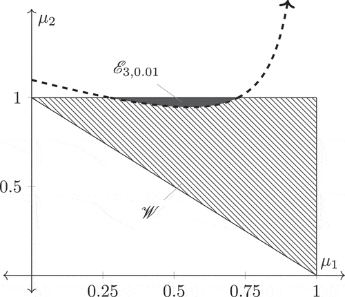
as it is shown in Figure 1.

Figure 1. The region of the set ${\mathcal{E}}_{3,0.01}$ in $\mathit{W}$.

Next, we indicate the cardinality of the set

$F_{\zeta }\{\mathit{m};({\mu }_1,{\mu }_2)\in {\mathcal{E}}_{\mathit{m},\mathit{\zeta }}\},$

for $\mathit{\zeta }\in \{0.1,0.001,0.00001,0.0000001\}$ in Figure 2 and for $\mathit{\zeta }\in \{\frac{1}{100},\frac{1}{400},\frac{1}{700},\frac{1}{1000}\}$ in Figure 3 via heat map representations. Note that the sidebar of subplots are the actual cardinalities. We can note from the figures that the cardinality of $F_{\zeta }$ changes from dark blue to dark red $-$ i.e. it increases from small to large.

Figure 2. Heat maps for $F_{\zeta }$ for $\mathit{\zeta }\in \{0.1,0.001,0.00001,0.0000001\}$.

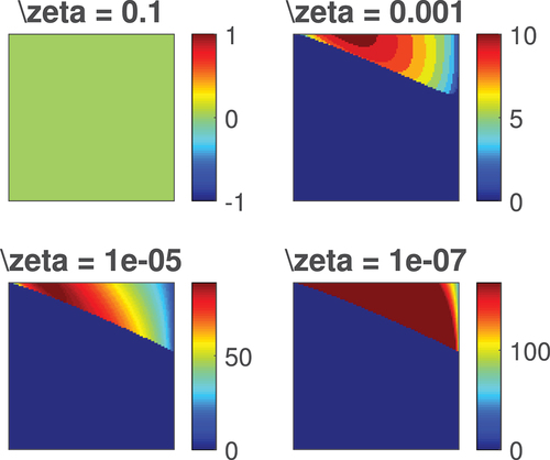
Figure 3. Heat maps for $F_{\zeta }$ for $\mathit{\zeta }\in \{\frac{1}{100},\frac{1}{400},\frac{1}{700},\frac{1}{1000}\}$.

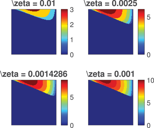
In particular, the change in the acuity of the boundaries of the heat map regions enables us to conclude the following results:

• $\underset{\mathit{\zeta }\to 0+}{lim}|F_{\zeta }|=+\mathrm{\infty }$. Particularly, it means that if we have $\mathit{f}:{\mathbb{N}}_a\to \mathbb{R}$ with

$\left({ }_{a+1}^{\mathrm{R}\mathrm{L}}{\mathrm{\nabla }}^{{\mu }_2}{}_a^{\mathrm{R}\mathrm{L}}{\mathrm{\nabla }}^{{\mu }_1}\mathit{f}\right)(\mathit{x})\stackrel{>}{=\phantom{{ }_x}}\$-\mathit{\zeta }\mathit{f}(\mathit{a}+1),$

then the number of points at which $(\mathrm{\nabla f})(\mathit{x})>0$ tends to $+\mathrm{\infty }$ when $\mathit{\zeta }\to 0^{+}$.

• If the negative lower bound on $\left({ }_{a+1}^{\mathrm{R}\mathrm{L}}{\mathrm{\nabla }}^{{\mu }_2}{}_a^{\mathrm{R}\mathrm{L}}{\mathrm{\nabla }}^{{\mu }_1}\mathit{f}\right)(\mathit{x})$ is not negative, then $\mathit{f}$ maybe increase for a long-time as in Corollary 3.1.

• It appears that,

$|{\mathcal{E}}_{\mathit{m},\mathit{\zeta }}\mathrm{\setminus }\{({\mu }_1,{\mu }_2)\mathit{W};{\mu }_2\stackrel{>}{=\phantom{{ }_x}}\$\frac{2-{\mu }_1}{2}\}|\approx 0,$

for a sufficiently small value of $\mathit{\zeta }$ and not too large value of $\mathit{m}$. In other words, if $\mathit{\zeta }\to 0^{+}$, then for plenty of time steps the admissible parameter space converges to the configuration of parameter space as $\mathit{\zeta }=0$ $-$ i.e.

${\mathcal{E}}_{\mathit{m},\mathit{\zeta }}\approx \{({\mu }_1,{\mu }_2)\mathit{W};{\mu }_2\stackrel{>}{=\phantom{{ }_x}}\$\frac{2-{\mu }_1}{2}\},$

for $\mathit{m}$ is not too large.

5. Concluding remarks

This study has dealt with analysing the sequential operator of order $({\mu }_2,{\mu }_1)\in (0,1)\times (0,1)$, where $0<{\mu }_2+{\mu }_1<1$ analytically. As a consequence, we have found the main formula for $(\mathrm{\nabla f})(\mathit{a}+\mathit{m})$ in Lemma 3.1 as an inequality. This helped us to find that $(\mathrm{\nabla f})(\mathit{a}+3).3\mathit{ex}=\mathit{x}0$ with four conditions as a preliminary main result. However, it was not the only aim of the article and we have continued by considering the set ${\mathcal{E}}_{\mathit{m},\mathit{\zeta }}$, which we have structured it from the inequality (3.1). We have found that this set is decreasing. Due to the decrease of this set we have then investigated that $(\mathrm{\nabla f})(\mathit{a}+\mathit{m})\mathit{\hspace{0.17em}}.3\mathit{ex}=\mathit{x}0$ on a finite time scale $\mathit{m}\in {\mathbb{N}}_2^{\tau }$, where $\mathit{\tau }\in {\mathbb{N}}_2$. On the other hand, even for small values $\mathit{m}$ and $0<\mathit{\zeta }$ we couldn’t analyse the set ${\mathcal{E}}_{\mathit{m},\mathit{\zeta }}$ accurately. Therefore, we have jumped for numerical simulations to estimate the set ${\mathcal{E}}_{\mathit{m},\mathit{\zeta }}$ numerically as we have demonstrated it graphically in the last section of the article based on the heat maps. We have concluded that the cardinality of $F_{\zeta }$ increases from small to large as shown in Figures 2–3 for different values of $\mathit{\zeta }$.

Extensions of our theory of the nabla sequential operators to more general fractional difference operators are underway, and constitute the focus of a promising research line, in which the researchers can use the following generalized articles (see Mohammed et al. 2021a; Mohammed and Abdeljawad 2023).

Acknowledgments

Researchers Supporting Project number (RSP2024R153), King Saud University, Riyadh, Saudi Arabia.

Disclosure statement

No potential conflict of interest was reported by the author(s).

References

- Abdeljawad T. 2018. Different type kernel h–fractional differences and their fractional h–sums. Chaos Solit Fract. 116:146–156. doi: 10.1016/j.chaos.2018.09.022.
- Abdeljawad T, Baleanu D. 2016. Discrete fractional differences with nonsingular discrete Mittag-Leffler kernels. Adv Differ Equ. 2016(1):1–5. doi: 10.1186/s13662-016-0949-5.
- Atici FM, Eloe PW. 2008. Initial value problems in discrete fractional calculus. Proc Amer Math Soc. 137(3):981–989. doi: 10.1090/S0002-9939-08-09626-3.
- Baleanu D, Wu GC, Bai YR, Chen FL. 2017. Stability analysis of Caputo-like discrete fractional systems. Commun Nonlinear Sci Numer Simul. 48:520–530. doi: 10.1016/j.cnsns.2017.01.002.
- Dahal R, Goodrich CS, Lyons B. 2021. Monotonicity results for sequential fractional differences of mixed orders with negative lower bound. J Differ Equ Appl. 27(11):1574–1593. doi: 10.1080/10236198.2021.1999434.
- Gholami Y, Ghanbari K. 2016. Coupled systems of fractional ∇-difference boundary value problems. Differ Eq Appl. 8(4):459–470. doi: 10.7153/dea-08-26.
- Goodrich CS, Jonnalagadda JM. 2021. Monotonicity results for CFC nabla fractional differences with negative lower bound. Anal (Berlin). 41(4):221–229. doi: 10.1515/anly-2021-0011.
- Goodrich CS, Lyons B. 2020. Positivity and monotonicity results for triple sequential fractional differences via convolution. Analysis. 40(2):89–103. doi: 10.1515/anly-2019-0050.
- Goodrich CS, Peterson AC. 2015. Discrete fractional calculus. (NY): Springer.
- Liu X, Du F, Anderson D, Jia B. 2020. Monotonicity results for nabla fractional h-difference operators. Math Meth Appl Sci. 1–21. doi: 10.1002/mma.6823.
- Mohammed PO. 2024. Some positive results for exponential-kernel difference operators of Riemann-Liouville type. Math Model Control. 4(1):133–140. doi: 10.3934/mmc.2024012.
- Mohammed PO, Abdeljawad T. 2023. Discrete generalized fractional operators defined using h-discrete Mittag-Leffler kernels and applications to AB fractional difference systems. Math Meth Appl Sci. 46(7):7688–7713. doi: 10.1002/mma.7083.
- Mohammed PO, Abdeljawad T, Hamasalh FK. 2021a. Discrete Prabhakar fractional difference and sum operators. Chaos Solit Fractals. 150:111182. doi: 10.1016/j.chaos.2021.111182.
- Mohammed PO, Abdeljawad T, Hamasalh FK. 2021b. On Riemann—Liouville and Caputo fractional forward difference monotonicity analysis. Mathemat. 9(11):1303. doi: 10.3390/math9111303.
- Mohammed PO, Almusawa MY. 2023. On analysing discrete sequential operators of fractional order and their monotonicity results. AIMS Math. 8(6):12872–12888. doi: 10.3934/math.2023649.
- Mohammed PO, Almutairi O, Agarwal RP, Hamed YS. 2022. On convexity, monotonicity and positivity analysis for discrete fractional operators defined using exponential kernels. Fractal Fract. 6(2):55. doi: 10.3390/fractalfract6020055.
- Mohammed PO, Goodrich CS, Hamasalh FK, Kashuri A, Hamed YS. 2022. On positivity and monotonicity analysis for discrete fractional operators with discrete Mittag–Leffler kernel. Math Methods In App Sci. 45(10):6391–6410. doi: 10.1002/mma.8176.
- Mozyrska D, Torres DFM, Wyrwas M. 2019. Solutions of systems with the Caputo–Fabrizio fractional delta derivative on time scales. Nonlinear Anal Hybrid Syst. 32:168–176. doi: 10.1016/j.nahs.2018.12.001.
- Wu G, Baleanu D. 2015. Discrete chaos in fractional delayed logistic maps. Nonlinear Dyn. 80(4):1697–1703. doi: 10.1007/s11071-014-1250-3.