The stabilizing effect of small prey immigration on competitive predator-prey dynamics

ABSTRACT

In this paper, we propose competitive predator-prey models with a small immigration into the prey. The dynamics of these models are investigated by addressing the boundedness, coexistence, and extinction conditions, as well as the local and global stability of equilibria. Immigrants stabilize the systems and increase the probability of coexistence. A Hopf bifurcation analysis shows that the model with Holling type II exhibits a Hopf bifurcation with respect to immigration parameter, but there is no bifurcation of the model with Holling type I. The numerical results support the theoretical results. Additionally, incorporating a few immigrants into the prey has a high sensitivity when the dynamic is periodic, but it has a lower sensitivity when the dynamic is stable. The obtained results can be biologically interpreted to improve the survival of species in the environment by adding immigrants. The rescue effect is considered as one of the implications in the real world that interpret the obtained results in this study.

KEYWORDS AND PHRASES:

• Holling Type
• prey predator model
• small immigrations

1. Introduction

A theoretical ecology has been developed by connecting mathematics and ecology to discuss many phenomena and ideas. To explain such phenomena, many predictions have been made. Mathematical modelling is one of the most effective methods for explaining the process and predicting its progress. Nevertheless, it remains a major challenge to define ecological principles and describe them mathematically (Murray 2002). In biological mathematics, numerous researchers have paid considerable attention to construct models of predator-prey relationships. Several ideas have been introduced to interpret and predict the dynamic behaviour of predator-prey interactions especially investigating the stability of these models such as (Huang et al. 2006; Samanta 2010, 2021; Sarwardi et al. 2011; Ali and Jazar 2013; Tripathi et al. 2014; Alebraheem and Hasan 2014; Panja and Mondal 2015; Molla et al. 2019; Wang et al. 2020; Saha and Samanta 2020; Mondal and Samanta 2020; Panja 2021, 2023; He and Li 2022; Dawud and Jawad 2022; Alebraheem and Yang 2023; Jawad and Al Nuaimi 2023). Based on the Lotka-Voltera model (Lotka 1925; Volterra 1926), this field evolved. Prey predator models have been studied and developed to make them more realistic by adding various external stimuli that mimic real-life effects in natural life. One of the most significant external stimuli is immigration.

In nature, many predator-prey systems do not exist in isolation, also there is a need to support some ecosystems that help to achieve stability in these ecosystems, which in turn maintains the continuity of species survival. The survival of the predator is closely linked to the presence of prey, and with increasing the predation rates, the existence of this ecosystem will be threatened. When addressing ecosystem threats, the impact of rescue phenomena on prey is a significant factor. Biological systems in which endangered ecosystems are at risk of extinction can be perceived as being saved by the rescue effect phenomenon. As a result, new creatures are being added to the ecosystem because of this support process or by supplying more suitable living conditions in their environment, those creatures will be able to live longer (Ovaskainen 2017).

From the previous paragraph, the effects of small immigration have a significant role to consider. In the literature, only limited recent research has investigated immigration impact to discuss its effects on prey predator dynamics. Sugie and Saito (Sugie and Saito 2012) constructed populations interacting spatially in a simple manner by adding constant immigration of Rosenzweig – MacArthur predator-prey model, their model assumed that using Holling type II as functional response and the prey population grows logistically. Their analytical findings explain that adding constant prey immigration to the system dampens the large fluctuations and stabilizes the coexistence equilibrium point globally.

Mukherjee (2016) studied the dynamics of a three-species system under the effect of immigration and refuge. His model includes two prey species and one predator species. For species that are not attacked by predators, he assumed a constant immigration rate. He showed in his results that immigration destabilizes the system. Tahara et al. (2018) studied the effect of small immigration on the asymptotic stability of the Lotka Voltera model. They concluded that by adding a small immigrant population to the prey or predator population, the system could be stabilized. Alebraheem (2021) discussed the effect of the oscillation of constant immigration of the prey on the dynamics of the predator-prey model with Crowley – Martin functional and numerical responses. By adding the oscillation of the prey’s immigration, he showed numerically how it exhibits stable fluctuations and increases the likelihood of coexistence. In addition, delay equations are used to build some models in this regard (Chen and Zhang 2013; Al-Darabsah et al. 2016; Zhu and Wei 2016; Samuel 2020). Diz-Pita and Victoria Otero-Espinar (2021) introduced a review of some recent advances in prey predator models; one of the main sections of this article is revision of immigration in prey predator models.

It is noticed from the previously mentioned studies that there is a discrepancy in the results between these studies, this is due to the nature of the models that formulate the interacted populations of these models. However, the leitmotif idea is that immigration stabilizes predator-prey populations. In contrast to previous studies, we introduce to the state of the art a novel predator-prey models by taking into account intraspecific competition in both species with a few immigrants added to the prey to study the dynamics of these models. Also, we will present some analytical and numerical results from our analysis that improve ecological stability and probability of survival as main contributions. These kinds of models without consideration of immigration are utilized by Alebraheem (2018), who describes the growth rate of species using the logistic equation for both species. In addition, two types of Holling types functional responses are utilized to study different environments especially using Holling type II, which has two different dynamics steady state and limit cycle in these kinds of predator- prey models. The rest of this paper is organized as follows. In Section 2, we present the competitive predator-prey models with a small immigration into prey. In Section 3, we analyse these models by considering the boundedness, Kolmogorov analyses, the local and global stability of equilibria, as well as a Hopf bifurcation. Numerical simulations are presented to explain and support the mathematical analysis in Section 4. In Section 5, we give a brief conclusion to this paper.

2. The construction of the models

In this section, we consider autonomous competitive predator-prey models with few prey immigrants to investigate their long-term effects. Holling types I and II are used to describe the functional and numerical responses. The densities of prey and predator species are symbolized by x and y, respectively, to describe the interactions between predator and prey. The parameters are explained in Table 1. The non-dimensional prey predator model with Holling type I is as follows:

Table 1. List of symbols with their biological meaning.

symbol	The meaning
r	Inherent growth rate of prey
k	Carrying capacity of the system
u	Death rate of predator
$\mathit{\alpha }$	Accessibility parameter of prey by a predator
h	Handling and digestion rates of the predator
e	Efficiency of converting consumed prey into predator birth
$\frac{m}{x}$	Few prey immigrants

(1) $\begin{array}{rl}& \frac{\mathit{dx}}{\mathit{dt}}=\mathit{rx}\left(1-\frac{x}{k}\right)-\mathit{\alpha xy}+\frac{m}{x}=N_1\left(\mathit{x},\mathit{y}\right),\\ & \frac{\mathit{dy}}{\mathit{dt}}=-\mathit{uy}+\mathit{e\alpha xy}-\mathit{e\alpha }{y}^2=N_2\left(\mathit{x},\mathit{y}\right).\end{array}$(1)

The non-dimensional prey predator model with Holling type II is as follows:

(2) $\begin{array}{rl}& \frac{\mathit{dx}}{\mathit{dt}}=\mathit{rx}\left(1-\frac{x}{k}\right)-\frac{\mathit{\alpha xy}}{1+\mathit{h\alpha x}}+\frac{m}{x}=M_1(\mathit{x},\mathit{y}),\\ & \frac{\mathit{dy}}{\mathit{dt}}=-\mathit{uy}+\frac{\mathit{e\alpha xy}}{1+\mathit{h\alpha x}}-\frac{\mathit{e\alpha }}{1+\mathit{h\alpha x}}{y}^2=M_2(\mathit{x},\mathit{y}),\end{array}$(2)

subject to initial conditions

$\mathit{x}(0)=x_0>0,\mathit{y}(0)=y_0>0$ and all the parameters are supposed to be positive and assuming $\mathit{m}<\mathit{k}$.

The biological significance of the terms and expressions in the model (1) and (2) are clarified as follows:

$\mathit{rx}(1-\frac{x}{k})$ represents the growth rate of prey that involves intraspecific competition. The terms $\mathit{\alpha xy}$ and $\frac{\mathit{\alpha xy}}{1+\mathit{h\alpha x}}$ indicate to the functional responses of Holling types I and II, respectively, which represent predator consumption of prey, while the terms $\mathit{e\alpha xy}$ and $\frac{\mathit{e\alpha xy}}{1+\mathit{h\alpha x}}$ represent the numerical responses of Holling types I and II, respectively, which indicate to changing predator density in response to prey consumption. $-\mathit{uy}$ represents predator death rate term. $\frac{\mathit{e\alpha }}{1+\mathit{h\alpha x}}{y}^2$ represents intraspecific competition between predators. $\frac{m}{x}$ represents small prey immigration term.

3. The analysis of the models

3.1. The boundedness of the models

Lemma 1.

(i) In the system (1), if $\mathit{\alpha }{x}^2\mathit{y}-\mathit{m}\ge 0$,the differential equation $\frac{\mathit{dx}}{\mathit{dt}}\le \mathit{rx}(1-\frac{x}{k})$.

(ii) In the system (2), if $\mathit{\alpha }{x}^2\mathit{y}-\mathit{m}\ge 0$, the differential equation $\frac{\mathit{dx}}{\mathit{dt}}\le \mathit{rx}(1-\frac{x}{k})$.

As the second part is a generalization of the first part, the proof of the first part is omitted and can be performed in the same manner.

Proof.

We can write the first equation in system (2) as follows:

(3) $\frac{\mathit{dx}}{\mathit{dt}}=\mathit{rx}\left(1-\frac{x}{k}\right)-\left(\frac{\alpha x^2\mathit{y}-\mathit{m}-\mathit{h\alpha mx}}{\mathit{x}(1+\mathit{h\alpha x})}\right)$(3)

From (3), we assume

(4) $\frac{\alpha x^2\mathit{y}-\mathit{m}-\mathit{h\alpha mx}}{\mathit{x}(1+\mathit{h\alpha x})}\ge 0$(4)

More simplification and since $\mathit{x}(1+\mathit{h\alpha x})>0$, we can get

(5) $\mathit{\alpha }{x}^2\mathit{y}-\mathit{m}-\mathit{h\alpha mx}\ge 0$(5)

Since $\mathit{h\alpha mx}\ge 0$, we can consider for both systems (1) and (2)

(6) $\mathit{\alpha }{x}^2\mathit{y}-\mathit{m}\ge 0$(6)

Under the condition (6), we can get that

(7) $\frac{\mathit{dx}}{\mathit{dt}}\le \mathit{rx}\left(1-\frac{x}{k}\right)$(7)

Theorem 2.

(i) All the solutions of system (1) that start in $R_{+}^2$ for $\mathit{t}\ge 0$ are ultimately bounded under the condition (6).

(ii) All the solutions of system (2) that start in $R_{+}^2$ for $\mathit{t}\ge 0$ are ultimately bounded under the condition (6).

We prove the second part that is a generalization of the first part, so the proof of the first part can be done in the same manner and therefore is omitted.

Proof.

For system (2), assume $(\mathit{x}(\mathit{t}),\mathit{y}(\mathit{t}))$ be any solution. Based on Lemma 1, we have

(8) $\frac{\mathit{dx}}{\mathit{dt}}\le \mathit{rx}\left(1-\frac{x}{k}\right).$(8)

The solution of the Equation (7)(7) $\frac{\mathit{dx}}{\mathit{dt}}\le \mathit{rx}\left(1-\frac{x}{k}\right)$(7) is $\mathit{x}(\mathit{t})=\frac{\mathit{k}{\mathit{e}}^{\mathit{t}+\mathit{kc}}}{-1+e^{\mathit{t}+\mathit{kc}}}$, $\mathit{c}$ is an integration constant. Then

(9) $\underset{\mathit{t}\to \mathrm{\infty }}{lim}sup\mathit{x}\left(\mathit{t}\right)\le \mathrm{k}\mathrm{\forall }\mathit{t}>0.$(9)

Now, we show that $\mathit{x}\left(\mathit{t}\right)+\mathit{y}\left(\mathit{t}\right)\le \mathit{\theta },\mathrm{\forall t}\ge 0$.

Consider $\mathit{J}(\mathit{t})\in C^1(R_{+}\to R_{+})$ as

$\mathit{J}(\mathit{t})=\mathit{x}\left(\mathit{t}\right)+\mathit{y}\left(\mathit{t}\right)>0.$

The derivative of J with respect to time (t) is

(10) $\frac{\mathit{dJ}}{\mathit{dt}}=\frac{\mathit{dx}}{\mathit{dt}}+\frac{\mathit{dy}}{\mathit{dt}},$(10)

(11) $\frac{\mathit{dJ}}{\mathit{dt}}=\mathit{rx}\left(1-\frac{x}{k}\right)-\frac{\mathit{\alpha xy}}{1+\mathit{h\alpha x}}+\frac{m}{x}-\mathit{uy}+\frac{\mathit{e\alpha xy}}{1+\mathit{h\alpha x}}-\frac{e\alpha y^2}{1+\mathit{h\alpha x}}.$(11)

Since ${lim}_{\mathit{t}\to \mathrm{\infty }}sup\mathit{x}\left(\mathit{t}\right)\le \mathit{k},$, $max\{\mathit{rx}(1-\frac{x}{k})\}=\frac{4\mathit{r}}{k}$ and cancelling some terms since all the variables and parameters are positive, then we can assume

(12) $\frac{\mathit{dJ}}{\mathit{dt}}\le \frac{4\mathit{r}}{k}+\frac{m}{k}-\mathit{uy}+\frac{\mathit{e\alpha ky}}{1+\mathit{h\alpha x}}-\frac{e\alpha y^2}{1+\mathit{h\alpha x}}+\mathit{J}-\mathit{J}$(12)

(13) $\frac{\mathit{dJ}}{\mathit{dt}}+\mathit{J}\le \frac{4\mathit{r}}{k}+\frac{m}{k}-\mathit{uy}+\frac{\mathit{e\alpha ky}}{1+\mathit{h\alpha k}}-\frac{e\alpha y^2}{1+\mathit{h\alpha k}}+\mathit{x}+\mathit{y}$(13)

The term $\left(1-\mathit{u}+\frac{\mathit{e\alpha k}}{1+\mathit{h\alpha k}}\right)\mathit{y}-\frac{e\alpha y^2}{1+\mathit{h\alpha k}}$ has maximum value $\frac{1+\mathit{e\alpha k}+\mathit{hk\alpha }-\mathit{u}{(1+\mathit{hk\alpha })}^2}{4\mathit{e\alpha }(1+\mathit{hk\alpha })}=\mathit{\gamma }$, then

(14) $\frac{\mathit{dJ}}{\mathit{dt}}\le \frac{4\mathit{r}}{k}+\frac{m}{k}+\mathit{k}+\mathit{\gamma },$(14)

$\mathrm{Let}\mathit{\eta }=\frac{4\mathit{r}}{k}+\frac{m}{k}+\mathit{k}+\mathit{\gamma }$

(15) $\frac{\mathit{dJ}}{\mathit{dt}}+\mathit{J}\le \mathit{\eta },$(15)

Thus,

$\mathit{J}\left(\mathit{t}\right)\le \mathit{\eta }+\mathit{J}\left(0\right)e^{-\mathit{t}}.$

for $\mathit{t}\to \mathrm{\infty }$, then $\mathit{J}\le \mathit{\eta }$. So, $\mathit{J}$ is bounded. As a result, all the solutions of (2) are contained within

(16) $\mathit{\omega }=\{(\mathit{x},\mathit{y})\in R_{+}^2:\mathit{J}=\mathit{\eta }+\mathit{\epsilon }\}.$(16)

Thus, the solution of system (2) is bounded.

□

3.2. Kolmogorov analyses

Kolmogorov type analysis states that the system of Kolmogorov type has a unique interior equilibrium point and this point has two possible dynamics whether asymptotically stable or a limit cycle that is asymptotically stable from the outside (Freedman 1980; Sigmund 2007). Kolmogorov analyses involve many conditions that are used to validate predator- prey models (Huang et al. 1995) and to attain the conditions of coexistence and extinction of predators (Freedman 1980), which the coexistence concept means analytically if $\mathit{x}(0)>0$ and ${lim}_{\mathit{t}\to \mathrm{\infty }}\mathit{x}(\mathit{t})>0$, while geometrically differential equation trajectories are defined as bounding away from the coordinate planes. Extinction concept that means if $\mathit{x}(0)>0$ implies $\mathit{x}(\mathit{t})=0$ for $\mathit{t}>0$, while geometrically differential equation trajectories are defined as touching the coordinate planes. Systems (1) and (2) are assigned to the Kolmogorov type.

For the analysis of system (1), we have

(17) $\begin{array}{rl}& \mathit{x}{\mathrm{A}}_1(\mathit{x},\mathit{y})=\mathit{x}\left(\mathit{r}\left(1-\frac{x}{k}\right)-\mathit{\alpha y}+\frac{m}{x^2}\right),\\ & \mathit{y}{\mathrm{B}}_1(\mathit{x},\mathit{y})=\mathit{y}(-\mathit{u}+\mathit{e\alpha x}-\mathit{e\alpha y}),\end{array}$(17)

and for the analysis of system (2), we have

(18) $\begin{array}{rl}& \mathit{x}{\mathrm{A}}_2(\mathit{x},\mathit{y})=\mathit{x}\left(\mathit{r}\left(1-\frac{x}{k}\right)-\frac{\mathit{\alpha y}}{1+\mathit{h\alpha x}}+\frac{m}{x^2}\right),\\ & \mathit{y}{\mathrm{B}}_2(\mathit{x},\mathit{y})=\mathit{y}(-\mathit{u}+\frac{\mathit{e\alpha x}}{1+\mathit{h\alpha x}}-\frac{\mathit{e\alpha }}{1+\mathit{h\alpha x}}\mathit{y}).\end{array}$(18)

We determine the carrying capacity of the environment and the minimum prey values until a small predator population is present in order to derive the conditions of coexistence and extinction. The carrying capacity represents the maximum sustainable population, which gives such systems to be more validated and realistic. Thus, they are expressed mathematically as follows:

For the analysis of system (17), the carrying capacity is obtained as follows:

$\mathrm{\exists \zeta }>0$ ${\mathrm{A}}_1(\mathit{\zeta },0)=0$, then the carrying capacity $\mathit{\zeta }$ is

(19) $\begin{array}{rl}& \mathit{\zeta }=\frac{1}{3}(\mathit{k}-\frac{2^{\frac{1}{3}}{k}^2\mathit{r}}{{(-27km{r}^2-2k^3{r}^3+3\sqrt{3}\sqrt{27k^2{m}^2{r}^4+4k^4\mathit{m}{r}^5})}^{\frac{1}{3}}}\\ & -\frac{{(-27km{r}^2-2k^3{r}^3+3\sqrt{3}\sqrt{27k^2{m}^2{r}^4+4k^4\mathit{m}{r}^5})}^{\frac{1}{3}}}{2^{\frac{1}{3}}\mathit{r}}\end{array}$(19)

The minimum prey value with a small predator population is obtained as follows:

$\mathrm{\exists \delta }>0B_1(\mathit{\delta },0)=0$, then the minimum prey value is

(20) $\mathit{\delta }=\frac{u}{\mathit{e\alpha }}.$(20)

The coexistence condition of the system (1) is satisfied if $\mathit{\zeta }>\mathit{\delta }$, one gets:

(21) $\begin{array}{rl}& \frac{1}{3}(\mathit{k}-\frac{2^{\frac{1}{3}}{k}^2\mathit{r}}{{(-27km{r}^2-2k^3{r}^3+3\sqrt{3}\sqrt{27k^2{m}^2{r}^4+4k^4\mathit{m}{r}^5})}^{\frac{1}{3}}}\\ & -\frac{{(-27km{r}^2-2k^3{r}^3+3\sqrt{3}\sqrt{27k^2{m}^2{r}^4+4k^4\mathit{m}{r}^5})}^{\frac{1}{3}}}{2^{\frac{1}{3}}\mathit{r}}>\frac{u}{\mathit{e\alpha }}\end{array}$(21)

However, if condition (21) is not met, then

(22) $\begin{array}{rl}& \frac{1}{3}(\mathit{k}-\frac{2^{\frac{1}{3}}{k}^2\mathit{r}}{{(-27km{r}^2-2k^3{r}^3+3\sqrt{3}\sqrt{27k^2{m}^2{r}^4+4k^4\mathit{m}{r}^5})}^{\frac{1}{3}}}\\ & -\frac{{(-27km{r}^2-2k^3{r}^3+3\sqrt{3}\sqrt{27k^2{m}^2{r}^4+4k^4\mathit{m}{r}^5})}^{\frac{1}{3}}}{2^{\frac{1}{3}}\mathit{r}}\le \frac{u}{\mathit{e\alpha }}\end{array}$(22)

and the predator is extinct.

For the analysis of system (18), we proceed in a similar way. We find that the carrying capacity of system (2) satisfies the same condition (i.e. condition (19)) as in system (1).

The minimum prey value with a small predator population is obtained as follows:

$\mathrm{\exists \gamma }>0{\mathrm{B}}_2(\mathit{\gamma },0)=0$, then the minimum prey value is

(23) $\mathit{\gamma }=\frac{u}{\mathit{e\alpha }-\mathit{uh\alpha }}.$(23)

The coexistence condition of the system (2) is satisfied if $\mathit{\zeta }>\mathit{\delta }$, one gets:

(24) $\begin{array}{rl}& \frac{1}{3}(\mathit{k}-\frac{2^{\frac{1}{3}}{k}^2\mathit{r}}{{(-27km{r}^2-2k^3{r}^3+3\sqrt{3}\sqrt{27k^2{m}^2{r}^4+4k^4\mathit{m}{r}^5})}^{\frac{1}{3}}}\\ & -\frac{{(-27km{r}^2-2k^3{r}^3+3\sqrt{3}\sqrt{27k^2{m}^2{r}^4+4k^4\mathit{m}{r}^5})}^{\frac{1}{3}}}{2^{\frac{1}{3}}\mathit{r}}>\frac{u}{\mathit{e\alpha }-\mathit{uh\alpha }}\end{array}$(24)

However, if condition (24) is not met, then

(25) $\begin{array}{rl}& \frac{1}{3}(\mathit{k}-\frac{2^{\frac{1}{3}}{k}^2\mathit{r}}{{(-27km{r}^2-2k^3{r}^3+3\sqrt{3}\sqrt{27k^2{m}^2{r}^4+4k^4\mathit{m}{r}^5})}^{\frac{1}{3}}}\\ & -\frac{{(-27km{r}^2-2k^3{r}^3+3\sqrt{3}\sqrt{27k^2{m}^2{r}^4+4k^4\mathit{m}{r}^5})}^{\frac{1}{3}}}{2^{\frac{1}{3}}\mathit{r}}\le \frac{u}{\mathit{e\alpha }-\mathit{uh\alpha }}\end{array}$(25)

and the predator is extinct.

From this analysis, we deduce the following propositions and corollaries:

Proposition 3.

There is a coexistence between predator and prey in the system (1) if the condition (21) is satisfied.

Corollary 4.

There is an extinction of the predator under condition (22).

Proposition 5.

There is a coexistence between predator and prey in the system (2) if the condition (24) is satisfied.

Corollary 6.

In the system (2), there is an extinction of the predator under the condition (25).

3.3. The existence of equilibria and local and global stability analysis

In this subsection, we show the existence of nonnegative equilibria and study local and global stability. It is noticed that the systems (1) and (2) have two equilibrium points for each system that are nonnegative and biologically feasible.

3.3.1. Equilibria of system (1)

$E_f(\mathit{x}\ne 0,\mathit{y}=0)$ that is called the predator free equilibrium point, and while $E_c(\mathit{x}\ne 0,\mathit{y}\ne 0)$ we symbolize $E_c(\dot{x},\dot{y})$, it is called the coexistence equilibrium point. The predator free equilibrium point with Holling type I $E_{\mathit{fI}}(\mathit{x},0)$ is found by substituting $\mathit{y}=0$ in the system (1), then we get

(26) $-\frac{r}{k}{x}^3+\mathit{r}{x}^2+\mathit{m}=0$(26)

By using Descartes’ rule of signs, if the sequence of signs of equation (26)(26) $-\frac{r}{k}{x}^3+\mathit{r}{x}^2+\mathit{m}=0$(26) is $\left(-,+,+\right)$ and changes once, then there is only one positive root. This positive root, denoted as $\mathit{\zeta }$, is calculated in condition (19).

The coexistence equilibrium point of the system (1) $E_{\mathit{cI}}(\mathit{x}\ne 0,\mathit{y}\ne 0)$ that we symbolize $E_{\mathit{cI}}(\dot{x},\dot{y})$, it is gotten as follows:

(27) $-\left(\frac{r}{k}+\mathit{\alpha }\right){\dot{x}}^3+\left(\mathit{r}+\frac{u}{e}\right){\dot{x}}^2+\mathit{m}=0$(27)

and

(28) $\dot{y}=\frac{-u+e\alpha \dot{x}}{\mathit{e\alpha }}$(28)

By using Descarte’s rule of signs and the sequence of signs is $\left(-,+,+\right)$ of Equation (27)(27) $-\left(\frac{r}{k}+\mathit{\alpha }\right){\dot{x}}^3+\left(\mathit{r}+\frac{u}{e}\right){\dot{x}}^2+\mathit{m}=0$(27) that changes once, then there is only one positive root. $\dot{y}$ is a positive, if

(29) $\mathit{e\alpha }\dot{x}>\mathit{u}.$(29)

Proposition 7.

As long as the condition (29) holds, the coexistence equilibrium point $E_{\mathit{cI}}(\dot{x},\dot{y})$ exists.

Theorem 8.

Under the following conditions:

(30) $\bullet \frac{2\mathit{r\zeta }}{k}+\frac{m}{{\zeta }^2}>\mathit{r},$(30)

(31) $\bullet \mathit{u}>\mathit{e\alpha \zeta },$(31)

the equilibrium point $E_{\mathit{fI}}\left(\mathit{x},0\right)$ is locally asymptotically stable.

Proof.

By substituting $\mathit{x}=\mathit{\zeta }\ne 0$ and $\mathit{y}=0$, then the Jacobian matrix of system (1) is□

$\mathit{J}\left(\mathit{x},0\right)=\left[\begin{array}{cc}\mathit{r}-\frac{2\mathit{r\zeta }}{k}-\frac{m}{{\zeta }^2}& -\mathit{\alpha \zeta }\\ 0& -\mathit{u}+\mathit{e\alpha \zeta }\\ \mathit{\hspace{0.17em}}& \mathit{\hspace{0.17em}}\end{array}\right].$

The eigenvalues are ${\lambda }_1=\mathit{r}-\frac{2\mathit{r\zeta }}{k}-\frac{m}{{\zeta }^2}\mathrm{and}{\lambda }_2=-\mathit{u}+\mathit{e\alpha \zeta }$

Then, the eigenvalues are negative if $\frac{2\mathit{r\zeta }}{k}+\frac{m}{{\zeta }^2}>\mathit{r}$ and $\mathit{u}>\mathit{e\alpha \zeta }$.

So, $E_{\mathit{fI}}\left(\mathit{x},0\right)$ is locally asymptotically stable under the conditions (30) and (31).

Theorem 9.

The coexistence equilibrium point is globally asymptotically stable in $R_{+}^2$, whenever it exists.

Proof.

Assume $\mathit{G}\left(\mathit{x},\mathit{y}\right)=\frac{1}{\mathit{xy}}$ be a Dulac function, which is smooth in $R_{+}^2$

Let $N_1\left(\mathit{x},\mathit{y}\right)=\frac{\mathit{dx}}{\mathit{dt}}$ and $N_2\left(\mathit{x},\mathit{y}\right)=\frac{\mathit{dy}}{\mathit{dt}}$. Now, the Dulac function is multiplied by the prey equation of system (1) and taking the partial derivatives according to $\mathit{x}$, which gives:

(32) $\begin{array}{rl}& \mathit{G}{N}_1=\frac{1}{\mathit{xy}}\left(\mathit{rx}\left(1-\frac{x}{k}\right)-\mathit{\alpha xy}+\frac{m}{x}\right)\\ & \mathit{G}{N}_1=\frac{1}{y}\left(\mathit{r}-\frac{\mathit{rx}}{k}\right)-\frac{1}{\mathit{xy}}\mathit{\alpha xy}+\frac{1}{\mathit{xy}}\frac{m}{x}\\ & \mathit{G}{N}_1=\frac{r}{y}-\frac{\mathit{rx}}{\mathit{ky}}-\mathit{\alpha }+\frac{m}{y{x}^2}\end{array}$(32)

(33) $\frac{\mathrm{\partial }G{N}_1}{\mathrm{\partial x}}=-\frac{r}{\mathit{ky}}-\frac{2\mathit{m}}{x^3\mathit{y}}$(33)

In the same manner, the Dulac function is multiplied by the predator equation of system (1) and taking the partial derivatives according to $\mathit{y}$, we get:

(34) $\begin{array}{rl}& \mathit{G}{N}_2=\frac{1}{\mathit{xy}}(-\mathit{uy}+\mathit{e\alpha xy}-\mathit{e\alpha }{y}^2)\\ & \mathit{G}{N}_2=\frac{-\mathit{uy}}{\mathit{xy}}+\frac{\mathit{e\alpha xy}}{\mathit{xy}}-\frac{e\alpha y^2}{\mathit{xy}}\\ & \mathit{G}{N}_2=\frac{-\mathit{u}}{x}+\mathit{e\alpha }-\frac{\mathit{e\alpha y}}{x}\\ & \frac{\mathrm{\partial }G{N}_2}{\mathrm{\partial y}}=-\frac{\mathit{e\alpha }}{x}\end{array}$(34)

Thus,

(35) $\mathrm{\Delta }(\mathit{G}{N}_1,\mathit{G}{N}_2)=\frac{\mathrm{\partial }G{N}_1}{\mathrm{\partial x}}+\frac{\mathrm{\partial }G{N}_2}{\mathrm{\partial y}}=-\frac{r}{\mathit{ky}}-\frac{2\mathit{m}}{x^3\mathit{y}}-\frac{\mathit{e\alpha }}{x}.$(35)

Since $\mathit{x}>0$ and $\mathit{y}>0$ as well as all the parameters are positive, then $\mathrm{\Delta }(\mathit{G}{N}_1,\mathit{G}{N}_2)$ is negative in $R_{+}^2$. To complete the proof, Poincare- Bendixson theorem is applied, so the conditions of this theorem are checked $\left(\mathit{x},\mathit{y}\right)\in R_{+}^2$, $N_1\left(\mathit{x},\mathit{y}\right)\mathit{and}{N}_2\left(\mathit{x},\mathit{y}\right)$ are differentiable continuous functions, and the system (1) is bounded from Theorem 2. Therefore, by the Poincare- Bendixson theorem, the system (1) is globally stable whenever the coexistence equilibrium point exists.□

Theorem 10.

In $R_{+}^2$, the system (1) has no periodic dynamic.

Proof.

As the system (1) is globally stable in $R_{+}^2$ whenever the coexistence equilibrium point exists and by using the Bendixson-Dulac criterion, the system (1) has no periodic dynamic.□

3.3.2. Equilibria of system (2)

In the same manner, we get the predator free equilibrium point with Holling type II, which $E_{\mathit{fII}}(\mathit{x},0)$ is found by substituting $\mathit{y}=0$ in system (2), then we obtain

(36) $-\frac{r}{k}{x}^3+\mathit{r}{x}^2+\mathit{m}=0.$(36)

There is one positive root that is $\mathit{\zeta }$ that calculated in the condition (19).

The coexistence equilibrium point of the system (2) $E_{\mathit{cII}}(\mathit{x}\ne 0,\mathit{y}\ne 0)$ that we symbolize $E_{\mathit{cII}}(\ddot{x},\ddot{y})$, it is obtained as follows:

(37) $\mathit{hku\alpha }{x}^4+\left(\mathit{er}+\mathit{ek\alpha }-\mathit{e\alpha hkr}-\mathit{hk\alpha k}\right)x^3-\left(\mathit{erk}+\mathit{ku}\right)x^2-\mathit{ehkm\alpha x}-\mathit{ekm}=0$(37)

and

(38) $\ddot{y}=\frac{1}{\alpha }\left(\left(1-\frac{\ddot{x}}{\mathit{k}}\right)+\frac{m}{{\ddot{x}}^2}\right)\left(1+\mathit{h\alpha }\ddot{x}\right).$(38)

By using Descarte’s rule of signs and the sequence of signs is (-,-,+,+) of Equation (37)(37) $\mathit{hku\alpha }{x}^4+\left(\mathit{er}+\mathit{ek\alpha }-\mathit{e\alpha hkr}-\mathit{hk\alpha k}\right)x^3-\left(\mathit{erk}+\mathit{ku}\right)x^2-\mathit{ehkm\alpha x}-\mathit{ekm}=0$(37) that changes once, then there is only one positive root. $\ddot{y}$ is a positive, if

(39) $\mathit{k}>\ddot{x}.$(39)

Proposition 11.

As long as the condition (39) holds, the coexistence equilibrium point $E_{\mathit{cII}}(\ddot{x},\ddot{y})$ exists.

Theorem 12.

Under the following conditions:

(40) $\begin{array}{rl}\bullet & \frac{2\mathit{r\zeta }}{k}+\frac{m}{{\zeta }^2}>\mathit{r},(\mathrm{i}.\mathrm{e}.,\mathrm{condition}(30))\\ & \bullet \mathit{u}>\frac{\mathit{e\alpha \zeta }}{1+\mathit{h\alpha \zeta }},\end{array}$(40)

the equilibrium point $E_{\mathit{fII}}\left(\mathit{x},0\right)$ is locally asymptotically stable.

Proof.

By substituting $\mathit{x}=\mathit{\zeta }\ne 0$ and $\mathit{y}=0$, then the Jacobian matrix of system (2) is

$\mathit{J}\left(\mathit{x},0\right)=\left[\begin{array}{cc}\mathit{r}-\frac{2\mathit{r\zeta }}{k}-\frac{m}{{\zeta }^2}& \frac{-\mathit{\alpha \zeta }}{1+\mathit{h\alpha \zeta }}\\ 0& -\mathit{u}+\frac{\mathit{e\alpha \zeta }}{1+\mathit{h\alpha \zeta }}\\ \mathit{\hspace{0.17em}}& \mathit{\hspace{0.17em}}\end{array}\right]$

The eigenvalues are ${\lambda }_1=\mathit{r}-\frac{2\mathit{r\zeta }}{k}-\frac{m}{{\zeta }^2}$ and${\lambda }_2=-\mathit{u}+\frac{\mathit{e\alpha x}}{1+\mathit{h\alpha \zeta }}$, and then, the eigenvalues are negative if

$\frac{2\mathit{r\zeta }}{k}+\frac{m}{{\zeta }^2}>\mathit{r}\mathit{and}\mathit{u}>\frac{\mathit{e\alpha \zeta }}{1+\mathit{h\alpha \zeta }}.$

Therefore, the equilibrium point $E_{\mathit{fII}}\left(\mathit{x},0\right)$ is locally stable under the conditions (30) and (40).

□

Theorem 13.

The coexistence equilibrium point $E_{\mathit{cII}}(\ddot{x},\ddot{y})$ is locally asymptotically stable if the following conditions are satisfied:

(41) $\mathit{r}-\frac{2r\ddot{x}}{\mathit{k}}-\frac{\alpha \ddot{y}}{1+\mathit{h\alpha }\ddot{x}}+\frac{{\alpha }^2\mathit{h}\ddot{x}\ddot{y}}{{\left(1+h\alpha \ddot{x}\right)}^2}-\frac{m}{{\ddot{x}}^2}<0,$(41)

(42) $-\mathit{u}+\frac{e\alpha \ddot{x}-2\mathit{e\alpha }\ddot{y}}{1+\mathit{h\alpha }\ddot{x}}<0.$(42)

Proof.

The Jacobian matrix of the system (2) when substituting the coexistence equilibrium point $E_{\mathit{cII}}(\ddot{x},\ddot{y})$ is obtained as follows:

$\mathit{J}\left(\ddot{x},\ddot{y}\right)=\left[\begin{array}{cc}\mathit{r}-\frac{2r\ddot{x}}{\mathit{k}}-\frac{\alpha \ddot{y}}{1+\mathit{h\alpha }\ddot{x}}+\frac{{\alpha }^2\mathit{h}\ddot{x}\ddot{y}}{{\left(1+h\alpha \ddot{x}\right)}^2}-\frac{m}{{\ddot{x}}^2}& \frac{-\alpha \ddot{x}}{1+\mathit{h\alpha }\ddot{x}}\\ \frac{e\alpha \ddot{y}}{1+\mathit{h\alpha }\ddot{x}}-\frac{e{\alpha }^2\mathit{h}\ddot{x}\ddot{y}}{{\left(1+h\alpha \ddot{x}\right)}^2}+\frac{e{\alpha }^2\mathit{h}{\ddot{y}}^2}{{\left(1+h\alpha \ddot{x}\right)}^2}& -\mathit{u}+\frac{e\alpha \ddot{x}}{1+\mathit{h\alpha }\ddot{x}}-\frac{2e\alpha \ddot{y}}{1+\mathit{h\alpha }\ddot{x}}\\ \mathit{\hspace{0.17em}}& \mathit{\hspace{0.17em}}\end{array}\right].$

It is possible to simplify it as follows:

$\mathit{J}\left(\ddot{x},\ddot{y}\right)=\left[\begin{array}{cc}\mathit{r}-\frac{2r\ddot{x}}{\mathit{k}}-\frac{\alpha \ddot{y}}{1+\mathit{h\alpha }\ddot{x}}+\frac{{\alpha }^2\mathit{h}\ddot{x}\ddot{y}}{{\left(1+h\alpha \ddot{x}\right)}^2}-\frac{m}{{\ddot{x}}^2}& \frac{-\alpha \ddot{x}}{1+\mathit{h\alpha }\ddot{x}}\\ \frac{e\alpha \ddot{y}}{{\left(1+h\alpha \ddot{x}\right)}^2}+\frac{e{\alpha }^2\mathit{h}{\ddot{y}}^2}{{\left(1+h\alpha \ddot{x}\right)}^2}& -\mathit{u}+\frac{e\alpha \ddot{x}-2\mathit{e\alpha }\ddot{y}}{1+\mathit{h\alpha }\ddot{x}}\\ \mathit{\hspace{0.17em}}& \mathit{\hspace{0.17em}}\end{array}\right],$

which can be rewritten as follows:

$\mathit{J}\left(\ddot{x},\ddot{y}\right)=\left[\begin{array}{cc}{a}_{11}& -a_{12}\\ a_{21}& a_{22}\end{array}\right],$

where

$a_{11}=\mathit{r}-\frac{2r\ddot{x}}{\mathit{k}}-\frac{\alpha \ddot{y}}{1+\mathit{h\alpha }\ddot{x}}+\frac{{\alpha }^2\mathit{h}\ddot{x}\ddot{y}}{{\left(1+h\alpha \ddot{x}\right)}^2}-\frac{m}{{\ddot{x}}^2},$

$a_{12}=\frac{\alpha \ddot{x}}{1+\mathit{h\alpha }\ddot{x}},$

$a_{21}=\frac{e\alpha \ddot{y}}{{\left(1+h\alpha \ddot{x}\right)}^2}+\frac{e{\alpha }^2\mathit{h}{\ddot{y}}^2}{{\left(1+h\alpha \ddot{x}\right)}^2},$

$a_{22}=-\mathit{u}+\frac{e\alpha \ddot{x}-2\mathit{e\alpha }\ddot{y}}{1+\mathit{h\alpha }\ddot{x}}.$

Since $a_{12}<0$ and $a_{21}>0$, so $\left|\mathit{J}\left(\ddot{x},\ddot{y}\right)\right|>0$ and $\mathit{Trace}(\mathit{J}\left(\ddot{x},\ddot{y}\right))<0$, if $a_{11}<0$ and $a_{22}<0$.

Hence, the coexistence equilibrium point $\mathit{E}(\ddot{x},\ddot{y})$ is locally asymptotically stable under the conditions (41) and (42).□

Theorem 14.

The system (2) has a periodic dynamics in $R_{+}^2$.

Proof.

Assume $\mathit{G}\left(\mathit{x},\mathit{y}\right)=\frac{1}{\mathit{xy}}$ be a Dulac function, which is smooth in $R_{+}^2$

Let $M_1\left(\mathit{x},\mathit{y}\right)=\frac{\mathit{dx}}{\mathit{dt}}$ and $M_2\left(\mathit{x},\mathit{y}\right)=\frac{\mathit{dy}}{\mathit{dt}}$.

Now, the Dulac function is multiplied by the prey equation of system (2) and taking the partial derivatives according to $\mathit{x}$, which gives:

(43) $\begin{array}{rl}& \mathit{G}{M}_1=\frac{1}{\mathit{xy}}\left(\mathit{rx}\left(1-\frac{x}{k}\right)-\frac{\mathit{\alpha xy}}{1+\mathit{h\alpha x}}+\frac{m}{x}\right)\\ & \mathit{G}{M}_1=\frac{1}{y}\left(\mathit{r}-\frac{\mathit{rx}}{k}\right)-\frac{1}{\mathit{xy}}\frac{\mathit{\alpha xy}}{(1+\mathit{h\alpha x})}+\frac{1}{\mathit{xy}}\frac{m}{x}\\ & \mathit{G}{M}_1=\frac{r}{y}-\frac{\mathit{rx}}{\mathit{ky}}-\frac{\alpha }{1+\mathit{h\alpha x}}+\frac{m}{y{x}^2}\end{array}$(43)

In the same manner, the Dulac function is multiplied by the predator equation of system (2) and taking the partial derivatives according to $\mathit{y}$, we get:

(44) $\frac{\mathrm{\partial }G{M}_1}{\mathrm{\partial x}}=-\frac{r}{\mathit{ky}}+\frac{h{\alpha }^2}{{\left(1+\mathit{h\alpha x}\right)}^2}-\frac{2\mathit{m}}{x^3\mathit{y}}$(44)

(45) $\begin{array}{rl}& \mathit{G}{M}_2=\frac{1}{\mathit{xy}}(-\mathit{uy}+\frac{\mathit{e\alpha xy}}{1+\mathit{h\alpha x}}-\frac{\mathit{e\alpha }}{1+\mathit{h\alpha x}}{y}^2)\\ & \mathit{G}{M}_2=\frac{-\mathit{uy}}{\mathit{xy}}+\frac{\mathit{e\alpha xy}}{\mathit{xy}(1+\mathit{h\alpha x})}-\frac{e\alpha y^2}{\mathit{xy}(1+\mathit{h\alpha x})}\\ & \mathit{G}{M}_2=\frac{-\mathit{u}}{x}+\frac{\mathit{e\alpha }}{1+\mathit{h\alpha x}}-\frac{\mathit{e\alpha y}}{\mathit{X}\left(1+\mathit{h\alpha x}\right)}\\ & \frac{\mathrm{\partial }G{M}_2}{\mathrm{\partial y}}=-\frac{\mathit{e\alpha }}{\mathit{x}\left(1+\mathit{h\alpha x}\right)}\end{array}$(45)

Thus,

(46) $\mathrm{\Delta }(\mathit{G}{M}_1,\mathit{G}{M}_2)=\frac{\mathrm{\partial }G{M}_1}{\mathrm{\partial x}}+\frac{\mathrm{\partial }G{M}_2}{\mathrm{\partial y}}=-\frac{r}{\mathit{ky}}+\frac{h{\alpha }^2}{{\left(1+\mathit{h\alpha x}\right)}^2}-\frac{2\mathit{m}}{x^3\mathit{y}}-\frac{\mathit{e\alpha }}{\mathit{x}\left(1+\mathit{h\alpha x}\right)}$(46)

Since $\mathit{x}>0$ and $\mathit{y}>0$ as well as all the parameters are positive, then $\mathrm{\Delta }(\mathit{G}{M}_1,\mathit{G}{M}_2)$ changes sign and not equals to zero in $R_{+}^2$.

To complete the proof, Poincare- Bendixson theorem is applied, so the conditions of this theorem are checked $\left(\mathit{x},\mathit{y}\right)\in R_{+}^2,M_1\left(\mathit{x},\mathit{y}\right)$ and $M_2\left(\mathit{x},\mathit{y}\right)$ are differentiable continuous functions, and the system (2) is bounded from Theorem 2. Through using the Poincare- Bendixson theorem, the system (2) has periodic dynamics.

3.4. Hopf bifurcation

A Hopf bifurcation is the point in which a system loses its stability and a periodic solution arises as a specific parameter varies. In this subsection, we study the Hopf bifurcation of the coexistence equilibrium point. Through the previous subsection, we get the system (1) is globally stable as shown through Theorem 9, so there is no bifurcation under any conditions. However, through depending on model parameters, the coexistence equilibrium point ($E_{\mathit{cII}}(\ddot{x},\ddot{y})$) of the system (2) can be stable or unstable. To study the Hopf bifurcation, we select $\mathit{m}$ as a bifurcation parameter.

Theorem 15.

System (2) undergoes a Hopf bifurcation around the coexistence equilibrium point ($E_{\mathit{cII}}(\ddot{x},\ddot{y})$) at the threshold $\mathit{m}=m_H$, where $m_H=\mathit{r}{\ddot{x}}^2-\frac{2r{\ddot{x}}^3}{\mathit{k}}-\frac{\alpha \ddot{y}{\ddot{x}}^2}{1+\mathit{h\alpha }\ddot{x}}\text{break}+\frac{{\alpha }^2\mathit{h}{\ddot{x}}^3\ddot{y}}{{\left(1+h\alpha \ddot{x}\right)}^2}-\mathit{u}{\ddot{x}}^2+\frac{e\alpha {\ddot{x}}^3-2\mathit{e\alpha }\ddot{y}{\ddot{x}}^2}{1+\mathit{h\alpha }\ddot{x}}$.

Proof.

The equilibrium point $E_{\mathit{cII}}(\ddot{x},\ddot{y})$ will be unstable case if $\mathit{m}>m_H$, then $\mathit{m}=m_H$ is the critical value where the stability of $E_{\mathit{cII}}(\ddot{x},\ddot{y})$ changes.

Assume that $\mathit{\lambda }=\mathit{A}(\mathit{m})+\mathit{B}(\mathit{m})\mathit{i}$ represents an eigenvalue of the Jacobian matrix $\mathit{J}((\ddot{x},\ddot{y});m_H))$. Thus, $\mathit{\lambda }$ is a purely imaginary number, when $\mathit{m}=m_H$ that occurs a Hopf bifurcation, we test these conditions by substituting $\mathit{m}$ by $m_H$, we can obtain that

$\mathit{Trace}(\mathit{J}((\ddot{x},\ddot{y});m_H))=0$, $\mathit{Det}(\mathit{J}((\ddot{x},\ddot{y});m_H))>0$ and $\frac{d(t\mathrm{race}(J((\ddot{x},\ddot{y});m_H)))}{\mathit{dm}}=\frac{-1}{{\ddot{x}}^2}\ne 0$. Thus, a Hopf bifurcation occurs at the point $\mathit{m}=m_H$.

□

4. Numerical simulations

This section clarifies the theoretical results by presenting the effect of small immigration into the prey on prey predator dynamics for the two systems (1) and (2). The Mathematica software package is used to perform numerical simulations with the assumption of parameter values that fit with the theoretical assumptions in Section 3 to satisfy the coexistence between prey and predator (i.e. Propositions 3 and 5) and the existence of coexistence equilibria (i.e. Propositions 7 and 11). There is only one dynamic of the system (1), which is a steady state as shown through Theorems 9 and 10, so one set of presumptive values for the parameters is selected and fixed, except for the immigration parameter, whose value is changed. Nevertheless, two different sets of presumptive values are picked out and fixed, but the immigration parameter value is changed. These sets are taken because there are two types of dynamics: steady state and periodic dynamics for the system (2), as demonstrated through Theorems 13 and 14.

In system (1), the supposed values of the parameters and the initial conditions are selected as follows:

$\mathit{r}=1,\mathit{k}=6,\mathit{\alpha }=0.8,\mathit{u}=0.5,\mathit{e}=0.4,\mathit{x}(0)=2,\mathit{y}(0)=1$

By using the supposed set of parameter values for the system described in (1), as illustrated in Figures 1, 2, and 3, the following results are observed:

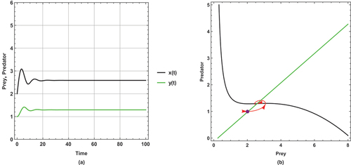
Figure 1. Prey predator dynamics of the system (1) when $(\mathit{m}=0)$: (a) time series (b) nullclines and phase portrait trajectories. Other parametric and initial values are: $\mathit{r}=1$, $\mathit{k}=6$, $\mathit{\alpha }=0.8$, $\mathit{u}=0.5$, $\mathit{e}=0.4$, $\mathit{x}(0)=2$, $\mathit{y}(0)=1$.

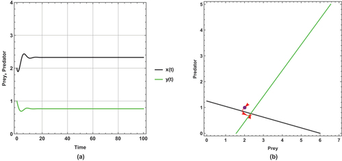
Figure 2. Prey predator dynamics of the system (1) when $(\mathit{m}=1.0)$: (a) time series (b) nullclines and phase portrait trajectories. Other parametric and initial values are: $\mathit{r}=1$, $\mathit{k}=6$, $\mathit{\alpha }=0.8$, $\mathit{u}=0.5$, $\mathit{e}=0.4$, $\mathit{x}(0)=2$, $\mathit{y}(0)=1$.

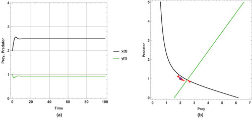
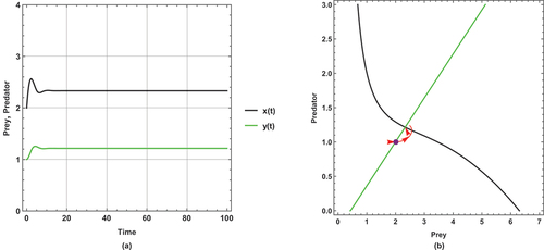
Figure 3. Prey predator dynamics of the system (1) when $(\mathit{m}=3.0)$: (a) time series (b) nullclines and phase portrait trajectories. Other parametric and initial values are: $\mathit{r}=1$, $\mathit{k}=6$, $\mathit{\alpha }=0.8$, $\mathit{u}=0.5$, $\mathit{e}=0.4$, $\mathit{x}(0)=2$, $\mathit{y}(0)=1$.

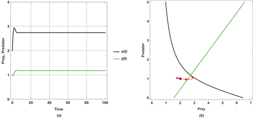
• The dynamical behaviours for all figures are steady state (i.e. no changes to the dynamical behaviours).

• There is a unique positive coexistence equilibrium point for each figure, which are Figure 1: (2.32759, 0.765086), Figure 2: (2.49391, 0.931412) and Figure 3: (2.74074,1.17824), respectively.

• With increasing small immigration, the density of prey and predator increases. The rise in density is explicitly displayed through the intersection between the prey and predator isoclines.

• Because the effect of small immigration is very less sensitive, large immigration parameter values are assumed in these cases.

In system (2), the first set of the parameter values and the initial conditions are given as follows:

$\mathit{r}=1,\mathit{k}=6,\mathit{\alpha }=3.25,\mathit{h}=0.40,\mathit{u}=0.45,\mathit{e}=0.5,\mathit{x}(0)=2,\mathit{y}(0)=1$

Using the first set of parameter values for the system (2) that are displayed in Figures 4, 5, and Figure 6, one gets the following results:

Figure 4. (a) Time series (b) nullclines and phase portrait trajectories of the first set of system (2) when $(\mathit{m}=0)$. Other parametric and initial values are: $\mathit{r}=1$, $\mathit{k}=6$, $\mathit{\alpha }=3.25$, $\mathit{h}=0.40$, $\mathit{u}=0.5$, $\mathit{e}=0.4$, $\mathit{x}(0)=2$, $\mathit{y}(0)=1$.

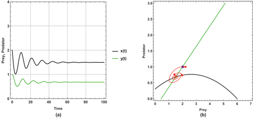
Figure 5. (a) Time series (b) nullclines and phase portrait trajectories of the first set of system (2) when $(\mathit{m}=0.5)$. Other parametric and initial values are: $\mathit{r}=1$, $\mathit{k}=6$, $\mathit{\alpha }=3.25$, $\mathit{h}=0.40$, $\mathit{u}=0.5$, $\mathit{e}=0.4$, $\mathit{x}(0)=2$, $\mathit{y}(0)=1$.

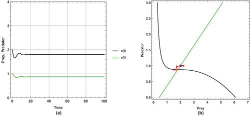
Figure 6. (a) Time series (b) nullclines and phase portrait trajectories of the first set of system (2) when $(\mathit{m}=2.0)$. Other parametric and initial values are: $\mathit{r}=1$, $\mathit{k}=6$, $\mathit{\alpha }=3.25$, $\mathit{h}=0.40$, $\mathit{u}=0.5$, $\mathit{e}=0.4$, $\mathit{x}(0)=2$, $\mathit{y}(0)=1$.

• The dynamical behaviour of Figure 4 begins with oscillation, but it stabilizes after some time. The other figures present steady state dynamical behaviour

• There is a unique positive coexistence equilibrium point for each figure. They are Figure 4: (1.4953, 0.680069), Figure 5: (1.80449, 0.877953) and Figure 6: (2.33083,1.21481), respectively.

• As immigration increases, prey and predator densities increase. The increased density is explicitly displayed through the intersection between the prey and predator isoclines.

• In this set of parameter values, the effect of the small immigration remains less sensitive, but it is more sensitive than the supposed set of parameter values for the system (1). As seen, it cancels any oscillation in Figure 4.

The second set of parameter values and the initial conditions in system (2) are as follows:

$\mathit{r}=1,\mathit{k}=8,\mathit{\alpha }=7.00,\mathit{h}=0.50,\mathit{u}=0.45,\mathit{e}=0.5,\mathit{x}(0)=2,\mathit{y}(0)=1$

Using the second set of parameter values for the system described in (2), as depicted in Figures 7, 8, and 9, the following results are concluded:

Figure 7. (a) Time series (b) nullclines and phase portrait trajectories of the second set of system (2) when $(\mathit{m}=0)$. Other parametric and initial values are: $\mathit{r}=1$, $\mathit{k}=8$, $\mathit{\alpha }=7.00$, $\mathit{h}=0.50$, $\mathit{u}=0.45$, $\mathit{e}=0.5$, $\mathit{x}(0)=2$, $\mathit{y}(0)=1$.

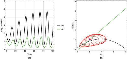
Figure 8. (a) Time series (b) nullclines and phase portrait trajectories of the second set of system (2) when $(\mathit{m}=0.1)$. Other parametric and initial values are: $\mathit{r}=1$, $\mathit{k}=8$, $\mathit{\alpha }=7.00$, $\mathit{h}=0.50$, $\mathit{u}=0.45$, $\mathit{e}=0.5$, $\mathit{x}(0)=2$, $\mathit{y}(0)=1$.

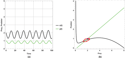
Figure 9. (a) Time series (b) nullclines and phase portrait trajectories of the second set of system (2) when $(\mathit{m}=1.5)$. Other parametric and initial values are: $\mathit{r}=1$, $\mathit{k}=8$, $\mathit{\alpha }=7.00$, $\mathit{h}=0.50$, $\mathit{u}=0.45$, $\mathit{e}=0.5$, $\mathit{x}(0)=2$, $\mathit{y}(0)=1$.

• Figure 7 shows a periodic dynamic with a large limit cycle and trajectory paths that approach the axes.

• In Figure 8, the dynamical behaviour remains periodic, but the limit cycle becomes smaller than in Figure 7 and the trajectories get away from the axes more than in Figure 7.

• However, the dynamical behaviour becomes steady state and has a unique positive coexistence equilibrium point (2.5861, 1.29378) as shown in Figure 9.

• This set of parameter values contains an important result: there is a change in the dynamical behaviour with increasing the small immigration from a periodic to a steady state, so this result ensures that the small immigration stabilizes the system and increases the probability of coexistence. This remarkable result is consistent with Theorem 14.

• This set of parameter values shows a high sensitivity to small immigration; this is demonstrated by changing the dynamical behaviour as small immigration is increased.

5. Conclusions

In this paper, a comprehensive study has been presented that discusses the small immigration effect on competitive predator-prey models with Holling types I and II. The model with Holling type I and without adding the small immigration factor is globally stable, and the model with Holling type II and without adding the small immigration factor has two different dynamics: steady state and periodic dynamics, respectively (Alebraheem 2018). The models are formed by adding a few prey immigrants to investigate their effects in the long term. In addition, competitive relationships are included in the model. The effect of immigration has been investigated in a few studies (Sugie and Saito 2012; Mukherjee 2016; Tahara et al. 2018; Alebraheem 2021). In contrast to the literature, in the model we investigate prey predator dynamics with few prey immigration and competitive relationships. The mathematical analysis of the systems (1) and (2) is displayed. One of the most significant features of these models is their boundedness, as proved in Theorem 2. The coexistence and extinction conditions are obtained, as seen from Propositions 3 and 5 as well as Corollaries 4 and 6. Each system has two nonnegative and biologically feasible equilibrium points. They are called the predator-free equilibrium point and the coexistence equilibrium point. Their existence is shown through Propositions 7 and 11. The dynamical behaviour of equilibrium points is studied in Theorems 8, 9, 10, 12, 13, and 14, which describe the local and global stability of the equilibrium points. A Hopf bifurcation analysis is investigated in Theorem 15, the theoretical results present that the model with Holling type II exhibits a Hopf bifurcation with respect to immigration parameter, but there is no bifurcation of the model with Holling type I. The numerical simulations explain and present the small immigration effect on prey. The addition of positive small-immigration acts as a stabilizing factor in competitive prey predator systems. The results are consistent with the literature (Sugie and Saito 2012; Tahara et al. 2018; Alebraheem 2021) and can be used to interpret stable prey and predator systems in nature because of a few immigrants over time. Increasing small immigration increases prey and predator densities. It also leads to a change in dynamic behaviour from periodic to stable dynamic, so this increases the probability of coexistence. The effect of the small immigration of prey has high sensitivity if the dynamic is periodic, but it is less sensitive when the dynamic is steady-stable. This study shows biologically that increasing small immigration of prey species will support the survival of both species in competitive predator models.

Acknowledgments

The first author extends the appreciation to the Deanship of Postgraduate Studies and Scientific Research at Majmaah University for funding this research work through the project number (R-2024-1032).

Disclosure statement

No potential conflict of interest was reported by the author(s).

References

- Al-Darabsah I, Tang X, Yuan Y. 2016. A prey-predator model with migrations and delays. Discrete Continuous Dyn Syst Ser B. 21(3):737–761. doi: 10.3934/dcdsb.2016.21.737.
- Alebraheem J. 2018. Relationship between the paradox of enrichment and the dynamics of persistence and extinction in prey-predator systems. Symmetry. 10(10):532. doi: 10.3390/sym10100532.
- Alebraheem J. 2021. Dynamics of a predator–prey model with the effect of oscillation of immigration of the prey. Diversity. 13(1):23. doi: 10.3390/d13010023.
- Alebraheem J, Hasan YA. 2014. Dynamics of a two predator–one prey system. Comput Appl Math. 33(3):767–780. doi: 10.1007/s40314-013-0093-8.
- Alebraheem J, Yang X. 2023. Predator interference in a predator–prey model with mixed functional and numerical responses. Pac J Math. 2023:1–13. Article ID 4349573. doi: 10.1155/2023/4349573.
- Ali N, Jazar M. 2013. Global dynamics of a modified leslie-gower predator-prey model with Crowley-Martin functional responses. J Appl Math Comput. 43(1–2):271–293. doi: 10.1007/s12190-013-0663-3.
- Chen Y, Zhang F. 2013. Dynamics of a delayed predator–prey model with predator migration. Appl Math Model. 37(3):1400–1412. doi: 10.1016/j.apm.2012.04.012.
- Dawud S, Jawad S. 2022. Stability analysis of a competitive ecological system in a polluted environment. Commun Math Biol Neurosci. 2022:1–34. doi: 10.28919/cmbn/7520.
- Diz-Pita É, Victoria Otero-Espinar M. 2021. Predator–prey models: a review of some recent advances. Mathematics. 9(15):1783. doi: 10.3390/math9151783.
- Freedman HI. 1980. Deterministic mathematical models in population ecology Vol. 57. (NY): Marcel Dekker Incorporated.
- He M, Li Z. 2022. Stability of a fear effect predator–prey model with mutual interference or group defense. J Biolog Dynamic. 16(1):480–498. doi: 10.1080/17513758.2022.2091800.
- Huang Y, Chen F, Zhong L. 2006. Stability analysis of a prey–predator model with Holling type III response function incorporating a prey refuge. Appl Math Comput. 182(1):672–683. doi: 10.1016/j.amc.2006.04.030.
- Huang L, Tang M, Yu J. 1995. Qualitative analysis of Kolmogorov-type models of predator-prey systems. Math Biosci. 130(1):85–97. doi: 10.1016/0025-5564(95)00038-F.
- Jawad SR, Al Nuaimi M. 2023. Persistence and bifurcation analysis among four species interactions with the influence of competition, predation and harvesting. Iraqi J Sci. 1369–1390. doi: 10.24996/ijs.2023.64.3.30.
- Lotka AJ. 1925. Elements of physical biology. Maryland (USA): Williams & Wilkins.
- Molla H, Sabiar Rahman M, Sarwardi S. 2019. Dynamics of a predator–prey model with Holling type II functional response incorporating a prey refuge depending on both the species. Int J Nonlinear Sci Numer Simul. 20(1):89–104. doi: 10.1515/ijnsns-2017-0224.
- Mondal S, Samanta GP. 2020. Dynamics of a delayed predator–prey interaction incorporating nonlinear prey refuge under the influence of fear effect and additional food. J Phys A: Math Theor. 53(29):295601. doi: 10.1088/1751-8121/ab81d8.
- Mukherjee D. 2016. The effect of refuge and immigration in a predator–prey system in the presence of a competitor for the prey. Nonlinear Anal Real World Appl. 31:277–287. doi: 10.1016/j.nonrwa.2016.02.004.
- Murray JD. 2002. Mathematical biology Vol. 2. (NY): springer. doi: 10.2307/40378655.
- Ovaskainen O. 2017. The interplay between immigration and local population dynamics in metapopulations. Ann Zool Fenn. 54(1–4):113–121. doi: 10.5735/086.054.0111.
- Panja P. 2021. Dynamics of a predator-prey model with Beddington-DeAngelis functional response, omnivory and predator switching. J Vibration Testing And System Dyn. 5(4):407–428. doi: 10.5890/JVTSD.2021.12.006.
- Panja P. 2023. Dynamics of a predator-prey model with group defense and exponential fading memory. Discontinuit, Nonlinearity, Complexit. 12(3):497–510. doi: 10.5890/DNC.2023.09.003.
- Panja P, Mondal SK. 2015. Stability analysis of coexistence of three species prey–predator model. Nonlinear Dyn. 81(1–2):373–382. doi: 10.1007/s11071-015-1997-1.
- Saha S, Samanta GP. 2020. A prey–predator system with disease in prey and cooperative hunting strategy in predator. J Phys A: Math Theor. 53(48):485601. doi: 10.1088/1751-8121/abbc7b.
- Samanta G. 2021. Deterministic, stochastic and thermodynamic modelling of some interacting species 4–13. Berlin: Springer.
- Samanta GP. 2010. A two-species competitive system under the influence of toxic substances. Appl Math Comput. 216(1):291–299. doi: 10.1016/j.amc.2010.01.061.
- Samuel AB. 2020. A predator-prey model with logistic growth for constant delayed migration. J Adv Math And Comput Sci. 35:51–61. doi: 10.9734/jamcs/2020/v35i330259.
- Sarwardi S, Haque M, Venturino E. 2011. Global stability and persistence in LG–Holling type II diseased predator ecosystems. J Biol Phys. 37(1):91–106. doi: 10.1007/s10867-010-9201-9.
- Sigmund K. 2007. Kolmogorov and population dynamics. In: Charpentier E, Lesne A Nikolski NK, Eds. Kolmogorov’s heritage in mathematics. Berlin, Heidelberg: Springer; p. 177–186.
- Sugie J, Saito Y. 2012. Uniqueness of limit cycles in a Rosenzweig-Macarthur model with prey immigration. SIAM J Appl Math. 72:299–316. doi: 10.1137/11084008X.
- Tahara T, Gavina MKA, Kawano T, Tubay JM, Rabajante JF, Ito H, Morita S, Ichinos G, Okabe T, Togashi T, et al. 2018. Asymptotic stability of a modified Lotka-Volterra model with small immigrations. Sci Rep. 8(1):7029. doi: 10.1038/s41598-018-25436-2.
- Tripathi J, Abbas S, Thakur M. 2014. Local and global stability analysis of a two prey one predator model with help. Commun Nonlinear Sci Numer Simul. 19(9):3284–3297. doi: 10.1016/j.cnsns.2014.02.003.
- Volterra V. 1926. Variazioni e fluttuazioni del numero d’individui in specie animali conviventi. in Memoire della Real Accademia Nazionale dei Lincei. Vol. 2. Taylor and Francis. p. 31–113. https://www.tandfonline.com/doi/full/10.1080/16583655.2020.1816027.
- Wang S, Yu H, Dai C, Zhao M. 2020. The dynamical behavior of a predator-prey system with Holling type II functional response and allee effect. J Comput And Appl Math. 11(5):407–425. doi: 10.4236/am.2020.115029.
- Zhu G, Wei J. 2016. Global stability and bifurcation analysis of a delayed predator–prey system with prey immigration. Electron J Qual Theory Differ Equ. 13(13):1–20. doi: 10.14232/ejqtde.2016.1.13.