Interval parameter estimation under model uncertainty

Abstract

This paper is devoted to the estimation of parameters of linear multi-output models with uncertain regressors and additive noise. The uncertainty is assumed to be described by intervals. Outer-bounding interval approximations of the non-convex feasible parameter set for uncertain systems are obtained. The method is based on the calculation of the interval solution for an interval system of linear algebraic equations and provides parameter estimators for models with a large number of measurements.

Keywords:

• Interval uncertainty
• interval equations
• uncertain model
• parameter estimation
• parameter bounding

1. Introduction

The set-membership estimation framework for uncertain systems has attracted much attention during the past few decades. It is an alternative to the stochastic approach where some prior information on the statistical distribution of errors is needed, because only bounds on uncertainty in system parameters and signals are required. This assumption is often much more acceptable in practice. Various types of compact sets (intervals, polytopes, ellipsoids, etc.) are usually used to characterize these bounds. They are called the membership set constraints on uncertain variables.

The parameter estimation problem for uncertain dynamic systems is one of the most natural in this context. The problem is to determine bounds or set constraints on system parameters based on output measurements, the model structure and bounds on uncertain variables. In this paper we focus on the so-called interval type of uncertainty. This means that each component of an uncertain vector or matrix is assumed to belong to a known finite interval. Although the description is natural and simple [1], combinatorial difficulties may become so severe as to make estimation intractable especially in the multidimensional case. The goal of the paper is to construct an effective interval parameter estimator for an uncertain multi-output static system that can be used with large sets of data.

Consider a linear regression model under interval uncertainty

where

is an unknown parameter vector,

denotes a vector of results of measurements,

is a matrix of regressors and

is an unknown vector of measurement errors. The classical parameter bounding approach is based on the assumption that the matrix C is known precisely, while the vector w is bounded and lies in the box

where

and

are known. This inclusion is understood componentwise. For instance, the set of all feasible parameter vectors x compatible with a single measurement

is the strip between two hyperplanes

The sequence of measurements y ₁, …, y_m then provides a convex polytope

. A number of methods has been developed to characterize this polytope or to construct outer-bounding approximations of it (see [2,3,4,5,6]).

The present paper deals with the more general problem of where the matrix of regressors is also uncertain, i.e. C∈C, and C is an interval matrix (

). This situation arises in many real-life problems when we do not have complete information concerning the plant. Furthermore, weakly non-linear systems can be treated in the same manner if non-linearity is replaced by uncertainty. Particular cases of this problem have been considered in the literature [3,7,8]. Any matrix or vector is said to belong to the interval family if its elements are from some real intervals [a;b], a ⩽ b. The standard notation

indicates the space of all interval (m × n) -matrices and

is the space of all n-dimensional interval vectors. The presence of matrix uncertainty in the model leads to serious difficulties due to the non-convexity of the resulting set constraints. In [9,10] ellipsoidal techniques were applied to state and parameter estimation for linear models with matrix uncertainty where non-convexity of reachable and feasible parameter sets was pointed out. The main purpose of this article is to apply an interval technique to parameter estimation. The basic tool for this is the interval solution of linear interval systems of equations.

The paper is organized as follows. Section 2 states the problem in detail. The scalar-measurement case is considered in section 3. In the multi-dimensional case the idea is to split a given linear model into a number of interval systems of linear algebraic equations. A simple method for solving these systems is proposed, which easily computes an optimal interval solution for moderate-scale problems (Section 4.2) whereas for large-scale problems effective interval over-bounding solutions are obtained (Section 4.3). The resulting method for parameter bounding is finally described in section 5.

2. Problem statement

Consider a multi-output model with measurement noise and uncertainty in the matrix of regressors

where

,

,

and

. The number of measurements is usually much larger than the dimension of the parameter vector, so

. Assume

The infinity norms of matrices and vectors are equal to the maximal absolute value of their elements, i.e.

Inequality (4) describes a particular case of interval uncertainty when all components of ΔC or w have the same bounds. The matrix C, vector y and scalars ϵ, δ are assumed to be known. All vectors

satisfying (3) under the constraints (4) form the feasible parameter set

Assume that x∈X ₀, where

. The initial approximation X ₀ should be taken large enough to guarantee inclusion of all parameter vectors of interest. The problem is to construct a more accurate outer-bounding interval approximation for the vector x in accordance with the large number of measurements {y ₁, …, y_m } and model structure (3) – (4). In other words, we look for an interval vector

(preferably of minimal size) containing the intersection

.

3. Scalar observation

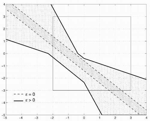
The single-measurement case (m = 1) is a good particular example of the parameter estimation. Set X for the scalar model

where

and

can be explicitly rewritten as

where

. Figure 1 depicts a typical shape of X ₁, which is non-convex for any ϵ > 0 (the region between two solid polygonal lines). This set reduces to a strip as ϵ→0. However it is convex in each orthant of

. Let E ^k be the k-th orthant of the vector space, k = 1, …, 2 ⁿ . If x∈E ^k for any fixed number k, the right-hand side of the inequality in (8) becomes a linear function and therefore

is a convex set.

Figure 1. Feasible parameter set (single measurement).

Assume x∈X ₀. Then the smallest interval vector X containing

can be found by solving a linear programming problem in each orthant of

. Indeed, the vector s ^k  = sign x for x∈E ^k is uniquely defined with elements

such that

. Thus

is a convex set given by linear constraints. Denote by e ^j the j-th unit coordinate vector of

, j = 1, …, n. Then the j-th lower and upper bounds on the intersection

are calculated by linear programming as

where (·,·) denotes the scalar product. Hence

gives an interval vector that is the minimal box containing

.

Notice however that the intersection of the set

with some orthants may be empty. The calculations in these orthants can obviously be omitted as long as the linear programming problem (10) turns out to become infeasible.

Further, let

. Then {E ^k :k∈K} represents a family of orthants containing

. Checking all orthants E ^k such that k∈K we obtain the inclusion

. Finally, take

gives the optimal interval approximation of

.

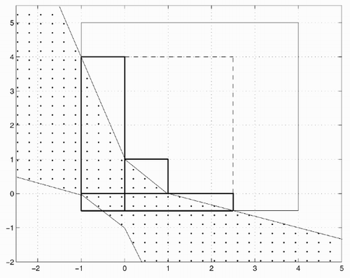
Example 1. Let X ₀ = ([ − 1,4],[ − 0.5,5]) ^T and y = 0, c = (1,1) ^T , ϵ = δ = 0.5. The set

is shown in figure 2 (shaded region). The auxiliary interval vectors X ^k are found via linear programming according to (10) in each orthant E ^k , k = 1, …, 4 (bold boxes). Then X = ([ − 1,2.5],[ − 0.5,4]) ^T .

Figure 2. Single-output interval parameter bounding.

In the multi-output case, one can consider the scalar observations recursively and apply the above linear programming procedure. However this technique becomes unsuitable for models with a large number of measurements (

). The main idea of the present paper is to consider blocks of n measurement equations in (3) and to treat each of them as a system of linear algebraic equations under interval uncertainties. A simple algorithm to obtain an interval solution for this system is described in the following section.

4. Interval system of linear algebraic equations

Let

, i.e. the number of parameters is equal to the number of observations. Then rewrite (3) in the form

with A = C, b = y, ΔA = ΔC and Δb =  – w such that ||ΔA||_∞ ⩽ ϵ, ||Δb||_∞ ⩽ δ.

The calculation of the interval solution for the interval system of equations (12) is a challenging problem in numerical analysis and robust linear algebra. This problem was first considered in the 1960s by Oettli and Prager [11]. Since then, the problem has attracted much attention and was developed in the context of the modelling of uncertain systems.

Assume that the matrix family

is non-singular (it contains no singular matrix) and that the interval vector is

. Then for any

and any

the ordinary linear system Ax = b has a unique solution. We are interested in a set

of all these solutions of the interval system:

Our main objective is to find an interval solution of the linear interval system (12), that is, to determine the smallest interval vector

containing all possible solutions (13). In other words, we want to embed the solution set

into the minimal box in

. This problem is known to be NP-hard [12] and complicated from a computational viewpoint for large-scale systems. Paper [11] shows how multiple linear programming can be used to obtain

; this line of research was continued in [13,14]. Iterative approaches have been established at this context as well as direct numerical methods that provide an over-bounding of

; see the monographs [15,16] and papers [17,18].

In this section we briefly describe a simple approach proposed in [19] for interval approximation of the solution set. Instead of employing linear programming in each orthant it is suggested to deal with a scalar equation. This method is based on Rohn's result [17] and simplifies his algorithm. In order to find the optimal interval estimate

of the solution set

, all vertices of its convex hull

should be obtained. The search of each vertex is via the solution of a scalar equation. In the case of large-scale systems we also provide a simple and fast procedure for over-bounding of the optimal interval solution.

4.1. The solution set

A detailed description of the solution set for the linear interval systems was given in the pioneering work by Oettli and Prager [11] for a general situation of interval uncertainty. In our case their result is reduced as follows.

Lemma 1 (Oettli & Prager [11]) The set of all admissible solutions of the system (12) is a non-convex polytope:

This result also follows from (8). The set

remains bounded as long as the interval matrix

is regular. This regularity is characterized by a non-singularity radius. For the interval family

this radius is equal to

see [20] for details. Recall that for any matrix G its (∞,1) -norm is defined as

Note also that the calculation of this norm is NP-hard.

While ϵ < ρ(A),

remains regular and

is bounded. If the solution set

lies in a given orthant of

, then it becomes convex, and the search for its interval approximation reduces to convex optimization. However this is no longer the case in most situations, and the problem then meets combinatorial difficulties.

4.2. Optimal interval estimates of the solution set

The problem is to determine exact lower

and upper

bounds on each component x_i of the vector

under the assumption that

. The approach is focused on searching for vertices of the convex hull

of the solution set

instead of employing linear programming in each orthant. The main base for this technique is the paper by Rohn [17], where a key result defining

was proved.

Let S be the set of vertices of the unit cube

. Consider a system of equations

for some s∈S, where a_i is the i-th row of the matrix A.

Lemma 2 (Rohn [17]). For a given nominal matrix A, let the interval family

be regular, i.e. all matrices in A are non-singular. Then the non-linear system of equations (17) has exactly one solution

for every fixed vector s∈S, and

.

To simplify the search for vertices x_s , introduce

. After change of the variables equalities (17) are converted to

Recall that s_i  =  ± 1; ∀i. The transformed solution set

is the affine image of

that is

. Note that

. For any positive value ϵ the intersection of

with each orthant of

is non-empty. Following Lemma 2 each orthant contains only one vertex of

that gives the solution of the system of equations (19) while the vector

specifies the choice of the orthant under consideration. Taking all vectors s from S we find all vertices for

. Moreover, (19) is equivalent to one scalar equation

where

,

and

. The function φ(τ) is defined for all τ ⩾ 0 and it is a convex piecewise linear function of τ.

Lemma 3 (see [19]) For any regular interval family

and any fixed vector s∈S the scalar equation (20) has a unique solution over [0,∞).

The solution τ* of (20) can be obtained using a simple iterative scheme, for example, Newton iterations

where we use the notation [α]₊ = max {0,α}. Procedure (21) converges to τ* for any initial τ₀ ⩾ 0 in a finite (no more than n) iterations. Finally, we can formulate the following theorem.

Theorem 1 The set

has 2 ⁿ vertices. Each vertex x_s can be found by solving the scalar equation (20) for a given vector s∈S by algorithm (21). Then

, where

and τ* is the solution of (20).

With these vertices we find the optimal lower and upper bounds for each component of x in the solution set

and finally

.

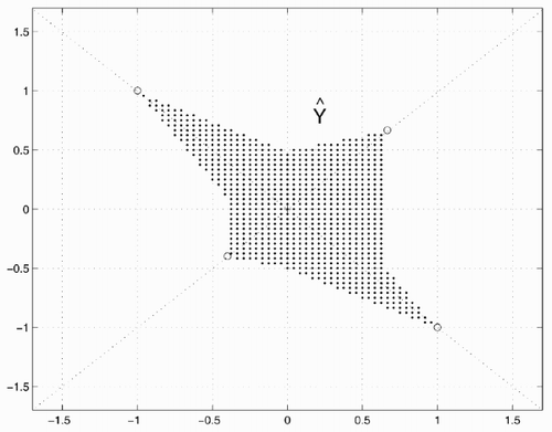
Example 2. For

,

, and ϵ = δ = 0.25 the solution set

is a bounded and non-convex polytope depicted in figure 3. Its image after the affine transformation

is shown in figure 4. All vertices of the convex hull

of the solution set with the variables

are represented by the vector s ^k with elements

and the value of τ from (20): y ¹ = (2/3, 2/3) ^T , y ² = ( – 1,1) ^T , y ³ = (1, – 1) ^T and y ⁴ = ( – 0.4, – 0.4) ^T . By inverse transformation

the vertices of

are obtained, and then it is trivial to find the interval bounds on

using (22). Finally X* = ([ – 1.5, 2.5], [ – 0.5, 1.5]) ^T .

Figure 3. The original solution set .

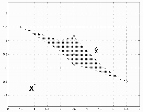
Figure 4. The transformed solution set .

4.3. Interval over-bounding technique

As already mentioned, the calculation of the optimal interval solution X* may be hard for large-dimensional problems. Hence, its simple interval over-bounding is of interest. This over-bounding is often said to be an interval solution of the interval system of equations as well. We provide below two such estimates.

According to the inequality

for the set

we write

where x* = A ^– 1 b. Therefore

All vectors

that belong to

thus also lie inside the ball in ∞-norm of radius γ. This ball is the first over-bounding interval estimate. In most cases (24) is the minimal cube centred at the origin containing

. The main difficulty here is to calculate the (∞,1) norm of A ^– 1; this is again an NP-hard problem. There exist tractable upper bounds for this norm; we use the simplest one: for any given matrix G with entries g_ij (i, j = 1, …, n) the value of

can always be approximated by a 1-norm:

Hence, the inequality (24) is replaced by

where ϵ should be less than

. An interval estimate for

implies an interval estimate for

. Indeed, x is an affine function of

and component-wise optimization for x_i on a cube can be performed explicitly. Then we arrive at the following result.

Theorem 2 The interval vector

with

contains the solution set

, where g_i is the i-th row of G = A ^– 1 while γ is the right-hand side of (24) or (26).

Thus the calculation of

given by (26), (27) is not involved, it does not lead to any combinatorial difficulties and does not require the solution of linear programming problems. Numerous examples confirm that this over-bounding solution is close to optimal. One such example is considered in [19] for the linear system Hx = b with H being a Hilbert matrix. Hilbert matrices are poorly conditioned even for small dimensions and for this reason it is a good test example in the framework of interval uncertainty. It was demonstrated in [19] that the over-bounding estimates (26), (27) and (24), (27) coincide in this case and give a very precise approximation of the smallest interval solution.

5. Large-scale interval parameter bounding

Assume now that

,

and

. The interval vector X ₀ is taken to be a prior approximation containing the parameter vector x. Let c_i be the i-th row of C. Below, we describe two recursive algorithms for an outer-bounding interval approximation of the intersection

.

In Algorithm 1, for simplicity, we assume m = Kn, where K is an integer.

Algorithm 1 Let k = 1. Assume

as an initial interval approximation.

1.	Step 1: Consider the interval system of linear equations from (3) that corresponds to the regressors c (kn-n + 1) , …, ckn . Compute the non-singularity radius ρ k for the nominal matrix A of this system. If ϵ < ρ k , then find its interval solution Xk, else (in particular, if A is singular) Xk is assumed to be infinitely large and go to step 3.
2.	Step 2: Find the smallest interval vector containing . Put .
3.	Step 3: If k = K, then terminate, else set k = k + 1 and go to step 1.

The interval solution X_k in step 1 can be calculated as described in section 2. For large-scale systems (e.g., n > 15) it can be obtained as a simple interval over-bounding, see section 3. The interval vector X computed by Algorithm 1 contains

. The main benefit of Algorithm 1 is its relatively low complexity. It requires the solution of K = m/n interval systems of equations.

Algorithm 2 Let k = 1. Assume X = X ₀ as an initial interval approximation.

1.	Step 1: Consider the interval system of linear equations from (3) corresponding to the regressors ck , … c k  + n – 1 . Compute the non-singularity radius ρ k for the nominal matrix A of this system. If ϵ < ρ k , then find its interval solution Xk , else go to step 3.
2.	Step 2: Find the smallest interval vector containing . Put .
3.	Step 3: If k = m – n + 1, then terminate, else set k = k + 1 and go to step 1.

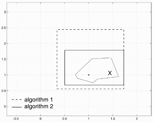
Algorithm 2 requires the solution of m – n + 1 interval systems of equations instead of m/n for Algorithm 1, but it provides a more accurate interval estimate.

Example 3 Let n = 2, m = 40 and x = (1,1) ^T be the parameter vector to be estimated, i.e. there are two parameters and 40 measurements in the model. The data are generated as follows. Take C be a (m × n) -matrix with rows c_i , which are samples of uniformly distributed vectors on the unit sphere. Interval uncertainty is defined by ϵ = 0.2 and δ = 0.5, and then ΔC = 2ε(rand(m,n) – 0.5) and w = 2δ(rand(m,1) – 0.5). The measurement vector

is taken to be y = (C + ΔC)x + w. These measurements are compatible with model (3) and given parameter vector x. Our purpose is to estimate x under given C, y. Algorithm 1 considers K = m/n = 20 linear interval systems. Let the initial interval approximation be X₀  = ([ − 5,5],[ − 5,5]) ^T . The interval estimator is constructed as an intersection of the optimal interval solutions for the linear interval systems; see figure 5. Algorithm 1 provides X₁ (dashed line box in figure 6) while Algorithm 2 computes a more precise interval approximation X₂ of the non-convex feasible parameter set X as the intersection of m – n + 1 = 39 optimal interval solutions for linear interval systems (solid line box in figure 6). Notice that the decrease in size of interval approximations in both recursive algorithms slows down after an initial rapid decrease. This effect often appears in parameter estimation.

Figure 5. Interval parameter estimator.

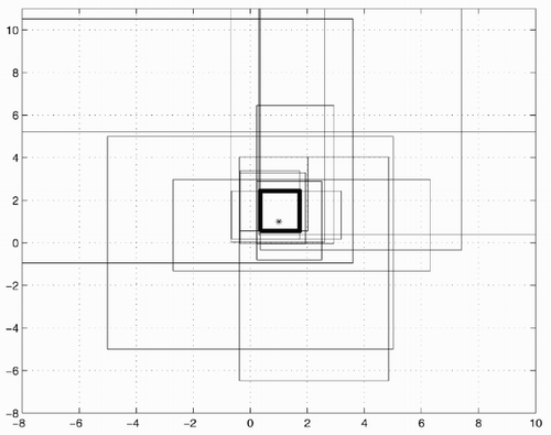
Figure 6. Interval approximations of X.

6. Conclusions

In this paper we considered the parameter estimation problem for linear multi-output models under interval uncertainty. The model uncertainty involves additive measurement noise vector and a bounded uncertain regressor matrix. Outer-bounding interval approximations of the non-convex feasible parameter set for this uncertain model are obtained. The algorithms described are based on the computation of interval solutions for square interval systems of linear equations. This approach allows computational difficulties to be avoided and provides a parameter estimator for models with a large number of measurements.

Acknowledgements

This work was supported in part by grant RFBR-02-01-00127. The work of S. A. Nazin was additionally supported by grant INTAS YSF 2002-181.

References

- Jaulin L Kieffer M Didrit O Walter E 2001 Applied Interval Analysis London Springer
- Walter , E and Piet-Lahanier , H . 1989 . Exact recursive polyhedral description of the feasible parameter set for bounded-error models . IEEE Transactions on Automatic Control , AC-34 : 911 – 914 .
- Walter E (Ed.) 1990 Special Issue on Parameter Identification with Error Bound Mathematics and Computing in Simulation 32
- Norton JP (Ed.) 1994 Special Issue on Bounded-Error Estimation, 1 International Journal of Adaptive Control and Signal Processing 8 1
- Norton JP (Ed.) 1995 Special Issue on Bounded-Error Estimation, 2 International Journal of Adaptive Control and Signal Processing 9 2
- Milanese M Norton J Piet-Lahanier H Walter E (Eds) 1996 Bounding Approaches to System Identification New York Plenum
- Cerone , V . 1993 . Feasible parameter set for linear models with bounded errors in all variables . Automatica , 29 : 1551 – 1555 .
- Norton JP 1999 Modal robust state estimator with deterministic specification of uncertainty In: A. Garulli, A. Tesi, A. Vicino (Eds) Robustness in Identification and Control London Springer pp. 62 – 71
- Chernousko , FL and Rokityanskii , DYa. 2000 . Ellipsoidal bounds on reachable sets of dynamical systems with matrices subjected to uncertain perturbations . Journal of Optimization Theory and Applications , 104 : 1 – 19 .
- Polyak , BT , Nazin , SA , Durieu , C and Walter , E . 2004 . Ellipsoidal parameter or state estimation under model uncertainty . Automatica , 40 : 1171 – 1179 .
- Oettli , W and Prager , W . 1964 . Compatibility of approximate solution of linear equations with given error bounds for coefficients and right-hand sides . Numerical Mathematics , 6 : 405 – 409 .
- Kreinovich , V , Lakeev , AV and Noskov , SI . 1993 . Optimal solution of interval linear systems is intractable (NP-hard) . Interval Computations , 1 : 6 – 14 .
- Cope , JE and Rust , BW . 1979 . Bounds on solutions of linear systems with inaccurate data . SIAM Journal of Numerical Analysis , 16 : 950 – 963 .
- Rust BW Burrus WR 1972 Mathematical Programming and the Numerical Solution of Linear Equations New York Elsevier
- Neumaier A 1990 Interval Methods for Systems of Equations Cambridge Cambridge University Press
- Higham NJ 1996 Accuracy and Stability of Numerical Algorithms Philadelphia SIAM
- Rohn , J . 1989 . Systems of linear interval equations . Linear Algebra and Its Applications , 126 : 39 – 78 .
- Shary , SP . 1995 . On optimal solution of interval linear equations . SIAM Journal of Numerical Analysis , 32 : 610 – 630 .
- Polyak , BT and Nazin , SA . Interval solution for interval algebraic equations . Mathematics and Computing in Simulation , 66 207 – 217 .
- Polyak BT 2003 Robust linear algebra and robust aperiodicity In: A. Rantzer and C. Byrnes (Eds) Directions in Mathematical System Theory and Optimization Berlin Springer pp. 249 – 260