Gender wage gap in Estonia: a non-parametric decomposition

Abstract

Estonia has the highest gender wage gap in the European Union and the highest degree of gender segregation by occupation and industry. Previous studies have found that most of the gap remains unexplained by personal and job characteristics. However, key job characteristics, occupation and industry, are usually imprecisely measured, leading to the question of whether all relevant characteristics have been properly taken into account in the decompositions. In this paper, we perform the decomposition of the wage gap to see how much of the wage gap remains unexplained after using more detailed data than has been common in previous studies (the Estonian Structure of Earnings Study data set), and discuss the related methodological challenges. Using a non-parametric method that takes into account differences in supports of distributions of male and female workers’ characteristics, we find that using more detailed data does not eliminate the unexplained wage gap: about half of the wage gap remains unexplained even using the full set of available variables.

Keywords:

• gender wage gap
• labour market segregation
• matching
• non-parametric decomposition

JEL Classification:

• J16
• D31
• J3
• J7

View addendum:

Addendum

1. Introduction

Estonia is the country with the highest gender wage gap in the European Union (EU). According to Eurostat's (2014) internationally comparable unadjusted gender wage gap indicator, the gap amounted to 30%,¹ substantially exceeding the next highest, that in Austria (23.7%). Yet, studies of the gender wage gap in Estonia have left a large portion of the gap unexplained. Although high levels of gender segregation by occupation and industry raise the question of whether these could be the reason behind the large gender wage gap, inclusion of these variables has so far been unable to explain more than a modest portion of the wage gap. In this paper, we examine whether a different methodology, accounting for differences in supports of male and female workers’ characteristics, and more detailed occupational and industry data could help explain more of the gender wage gap in Estonia.

There have not been many studies attempting to decompose the gender wage gap in Estonia into explained and unexplained portions. Rõõm and Kallaste (2004) find, using the Oaxaca–Blinder decomposition, that about two-thirds of the gender wage gap is unexplained. Anspal and Rõõm (2011), also using the same decomposition method, were able to explain only 10% of the wage gap. In Masso and Krillo's (2011) study, the explained Oaxaca–Blinder component makes up a maximum of 23% of the overall gap, depending on the year studied.² Christofides, Polycarpou, and Vrachimis (2013) estimate unexplained wage gaps for 26 European countries, including Estonia, using both Oaxaca and Ransom (1994) decomposition of the mean wage gap and the Melly (2005) quantile decomposition. They find that Estonia's gender wage gap is in large part unexplained – they are able to explain only 31–44% of the gap, depending on whether selection into employment is accounted for or not. Using quantile decomposition, they found no evidence of either ‘glass ceiling’ or ‘sticky floor’ effects, the gap being fairly similar across the wage distribution. Espenberg, Themas, and Masso (2013) use the Oaxaca–Blinder method to decompose the gender wage gap among university graduates and are able to explain 58% of the 25% wage gap among this group.

All of the gender wage gap decompositions for Estonia have been regression based. In applications of these methods, certain assumptions are made regarding the functional form of the wage equation which may not hold in practice and may result in misspecification. Namely, the effects of the explanatory variables on log wage are assumed to be additively separable. Thus, the effect of a college degree is typically estimated as a wage premium constant for all age groups, regions, or other values of explanatory variables. However, if particular combinations of characteristics have different effects from others, and if some combinations are observed for one gender but not for other, this approach is problematic. Ñopo (2008) gives the example of a married, highly educated worker in early 30s: it is much more difficult to find a female with these characteristics in the labour market than a male, and thus there is a problem of comparability.

In particular, if there is gender segregation by occupation or industry in the labour market (which is the case with Estonia, as shown below), the problem is exacerbated. It is difficult to ensure comparability if there are occupations that are dominated by or even exclusive to workers of one sex. A related problem is the measurement of occupation and industry in wage regressions: if the respective variables are not detailed enough, this may conceal the lack of common support in occupation or industry cells, while the underlying problem of incomparability – and the resulting risk of misspecification – remains. Studies on Estonia (e.g. Anspal & Rõõm, 2011; Christofides et al., 2013; Espenberg et al., 2013; Masso & Krillo, 2011; Rõõm & Kallaste, 2004) have included occupation and industry variables at the most general level (not more detailed than one-digit International Standard Classification of Occupations (ISCO) and Statistical Classification of Economic Activities in the European Community (NACE) classifications). However, given the high degree of gender segregation by occupation and industry in Estonia, a question remains as to whether the high levels of the unexplained wage gap could in fact also be ultimately due to the fact that males and females in Estonia have segregated into different and incomparable jobs, and whether this has been satisfactorily taken into account in existing studies.

For this reason, in this study, we perform the wage gap decomposition using a matching-based method developed by Ñopo (2008), which estimates the explained and unexplained gaps based on only those men and women who have identical combinations of characteristics (i.e. observations in common support of the distributions of those characteristics). This avoids the problem of differences in supports, thus enabling us to estimate the explained and unexplained components of the wage gap with more precision. In the decomposition exercise, the most detailed data on occupation and industry available (three-digit ISCO and two-digit NACE) are used.

In addition to the benefits of the matching-based decomposition method described above, another could be mentioned: the straightforward interpretation of the explained and unexplained wage gap estimates. In presenting estimates of the unexplained wage gap, obtained from regression models or decomposition exercises based on them, the unexplained gap is often presented as the differential between wages of male and female workers who have otherwise similar characteristics. This is only true if all assumptions made regarding the functional form of the wage regression hold, which might not be the case in reality (and if the relevant variables are measured with reasonable precision). In contrast, this simple interpretation of the unexplained gap is quite accurate in the case of matching-based decomposition. In addition, transforming parameter estimates from log wage regressions into the commonly understandable metric of per cent differentials is not trivial, as demonstrated by Blackburn (2007), among others.

Previous studies examining the effect of the level of occupational aggregation in gender wage gap decompositions include that of Kidd and Shannon (1996), who find that increasing the level of detail from 9 to 36 occupations increases the share of the explained part of the wage gap from 12.1% to 27.3%, based on Canadian data. In comparison, the novelty of the present study is in the level of detail of occupational data, which is much higher (we use 130 occupations and 79 industries) and also in our choice of method. We argue that because of the level of detail chosen, a matching-based method that explicitly confronts the issue of non-overlapping supports is more appropriate.

The paper is organized as follows. In Section 2, we give a brief overview of the methodology of Ñopo (2008) used in this paper. Section 3 describes the data set used and gives a descriptive analysis. Section 4 presents the results of the decomposition exercise. Section 5 concludes.

2. Methodology

To decompose the gender wage gap, we use Ñopo's (2008) method. The method recognizes that men's and women's supports of the distributions of individual characteristics may not overlap completely, and employs matching to calculate the explained and unexplained wage gaps (i.e. the parts of the wage gap due to differences in individual characteristics and differences in the returns to characteristics, respectively) on the basis of the sample restricted to common support only. In other words, explained and unexplained wage gaps are estimated only on the basis of those individuals whose particular combination of characteristics is also found among individuals of the opposite gender. In addition, the method also accounts for the part of the average gender wage gap due to out-of-support observations, as described below.

Ñopo (2008) starts out by expressing the gender wage gap, denoted as Δ, as follows: (1)

where Y denotes wages; M and F men and women, respectively; and denote the expected value of wages respectively for men and women, conditional on characteristics; and are cumulative distribution functions of individuals’ characteristics x ( and denote the respective probability measures); and and denote the supports of respectively men's and women's distributions of characteristics. As shown by Ñopo (2008), after partitioning the domains of the integrals and algebraic manipulation, this can further be expressed as (2)

where , that is, the probability measure of S under the distribution , and is defined analogously. Ñopo denoted the four components in Equation (2) as (3)

where and are, respectively, the explained (i.e. due to gender differences in characteristics) and unexplained (due to differences in returns to characteristics) portions of the gender wage gap. Thus, the interpretation of these components is analogous to that of the components from the Oaxaca–Blinder decomposition. However, as can be seen from the domains of the integrals of the middle two components of Equation (2), these components are defined over the common support only, that is, calculated on only on the basis of those individuals whose combinations of individual characteristics that are found among both men and women. The first component of Equation (3) is the portion of the wage gap that is due to the difference between wages of those males who have combinations of characteristics not found among females (i.e. out-of-support males who cannot be matched to females) and those males whose combinations of characteristics can be found among females and can be matched. Likewise, the last component, , is the portion of the wage gap attributable to the differences between out-of-support and in-support females. These components would be zero if there were no males or females with characteristics unmatched among the opposite sex, or if the average wages for out-of-support workers were the same as the average wages for in-support workers.

This non-parametric method has been successfully applied to decomposition of the wage gaps in studies such as Nicodemo and Ramos (2012), Ñopo, Daza, and Ramos (2012), and Görzig, Gornig, and Werwatz (2005), among others. The use of this method in this study is essentially similar, but differs in being applied to data that include detailed occupation and industry variables, greatly increasing the number of variables employed. This points out a drawback of using the Ñopo method, namely the so-called ‘curse of dimensionality’: as the number of variables increases, the share of men and women in common support could decrease markedly since men and women are matched on the specific combinations of all included variables. If the number of observations in common support is low, this widens the confidence intervals around the decomposition estimates, and there is also the possibility that the estimated unexplained and explained gaps do not account for much of the overall wage gap compared to out-of-support observations.

Nevertheless, we argue here that the curse of dimensionality here is not so much a shortcoming of the matching method as an aspect arising due to the choice of variables. If the use of very detailed variables is desired, then ignoring the problem of common support and using, for example, the Oaxaca method would not be a better solution but concealment of the problem, possibly resulting in biased estimates. As for the problem of wide confidence intervals, this may be possible to be remedied by using a large data set (as used in this study, described in the next section). There remains, however, the danger that the due to the small share of observations in common support, the share of explained and unexplained components in the overall wage gap turns out to be low. However, as we will see from the results of this study, this happens to be not the case with the Estonian data set used.

When using occupational variables, especially detailed ones, there is also the question of whether occupation should be interpreted as an exogenous variable – selection into occupations may involve gender specific barriers such as discrimination or societal attitudes. This complicates the interpretation of the explained and unexplained components in a decomposition involving detailed occupational variables: if it is found, for example, that the inclusion of more detailed occupational variables eliminates the unexplained gap, it would indeed be incorrect to interpret this as evidence of no labour market discrimination. If, however, a substantial unexplained gap remains (as is the case with Estonia, shown below), it is an indication that there exist gender inequalities that operate through different channels than occupational segregation. The decomposition thus remains informative with regard to the nature of the gender wage disparity.

3. Data

We use data from the Estonian Structure of Earnings Study (SES) for the year 2010. It is an employer survey that is carried out once in every four years by Statistics Estonia. The survey was conducted using a representative sample of 122,122 employees, at ages ranging from 15 to 91, from 10,872 establishments. The sample includes 19.2% of the total population of establishments. All of the establishments with at least 150 employees are included in the sample, but each of the establishments in this size group reports data on a sample drawn from its employees. A stratified (on the basis of industry) sample is drawn from establishments with less than 150 employees; these report on all of their employees.

The survey includes data on hourly earnings in the month of October in 2010. In addition, the data set includes the following background variables: sex; age; occupation; the highest successfully completed level of education and training; citizenship; whether the employee works full-time or part-time; type of employment contract; collective agreement coverage; ownership of the establishment (public or private); size of the establishment; industry; region of establishment; length of service in enterprise. Data on earnings do not include irregular bonuses, but data are collected separately for a number of different types of remuneration: overtime, special payments for shift work, annual bonuses, etc.

In this paper, we only consider hourly wage which includes pay for the month of October, overtime, night shift pay, monthly bonus, bonuses for difficult work conditions, bonuses for language skills, qualifications or tenure, and other such regular earnings, but not annual or irregular bonuses and payments. We limit our sample to full-time workers in order to avoid possible issues with measurement of working time (information on the number of hours was not available, only an indicator variable for full-time or part-time work). While leaving part-time work out of the purview of this study, we note that as in other countries, the topic of part-time work is very relevant to the gender wage gap also in Estonia. Part-time work is much more common for women than for men: in the Structure of Earnings Survey data set, 20% of women work part-time while only 9.99% of men work part-time.³ Krillo and Masso (2010) offer an excellent study of the part-time/full-time wage gap in Estonia, differentiating the effects by gender and also discussing the cyclical behaviour of the wage gaps.

The data set available for researchers includes industry on a two-digit level of NACE and occupation on a three-digit level of ISCO-08. Variables not available are collective agreement coverage, citizenship, region of the establishment.

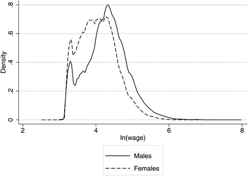
Next, we review the descriptive statistics. To start with wage, the dependent variable, we present kernel densities of men's and women's hourly wages (in natural logarithms) on Figure 1. The sample includes full-time employees only. As can be seen, the distribution of men's wages is located on the right compared to that of women's wages,⁴ in particular for wages higher than the local peak at about log wage 3.5 (corresponding to the monthly wage of 5000 Estonian kroons or EUR 320). For women, the density is much higher in the region between 3.5 and 4.3 (approximately corresponding to the monthly wage range of EEK 5000–10,000), while for men, the density is higher at log wages higher than 4.3. The raw wage gap (difference between men's and women's wages as a percentage of men's wages) in the sample is 30.6% in men's favour.

Figure 1. Kernel density of log wages by gender.

Source: Statistics Estonia, author's calculations.

Second, we look at the descriptive variables used in the decomposition, comparing averages for men and women (see Table 1). On average, women have a higher level of education than men: the share of women with a tertiary education is 27%, 6 percentage points higher than the corresponding figure for men.

Table 1. Means of the variables used in the study.

	Men	Women
Education
Primary	0.004	0.002
Secondary	0.78	0.73
Tertiary	0.21	0.27
Occupation
Armed forces occupations	0.02	0.001
Managers	0.12	0.06
Professionals	0.12	0.22
Technicians and associate professionals	0.16	0.20
Clerical support workers	0.03	0.09
Service and sales workers	0.08	0.22
Skilled agricultural, forestry, and fishery workers	0.001	0.001
Craft and related trades workers	0.23	0.05
Plant and machine operators, and assemblers	0.17	0.07
Elementary occupations	0.07	0.09
Industry
Mining and quarrying	0.02	0.003
Manufacturing	0.24	0.18
Electricity and gas supply	0.02	0.01
Water supply and waste management	0.01	0.005
Construction	0.13	0.01
Wholesale and retail trade	0.13	0.18
Transportation and storage	0.11	0.04
Accommodation and food service	0.01	0.04
Information and communication	0.04	0.02
Finance and insurance	0.01	0.03
Real estate	0.01	0.01
Professional, scientific, and technical activities	0.04	0.04
Administrative and support services	0.05	0.04
Public administration, defence, and social security	0.08	0.09
Education	0.04	0.15
Healthcare and social work	0.02	0.11
Arts, entertainment, and recreation	0.01	0.03
Other service activities	0.01	0.01
Firm size
1–9	0.18	0.13
10–49	0.27	0.23
50–249	0.27	0.30
250–499	0.08	0.10
500–999	0.07	0.08
1000+	0.12	0.17
Ownership
Public	0.21	0.38
Private	0.79	0.62

Source: Statistics Estonia, author's calculations.

The occupational structure of women's employment differs considerably from that of men. Indeed, an earlier report by the European Commission finds occupational segregation in Estonia to be the highest among the EU countries (European Commission 2012). The Duncan index of dissimilarity calculated on the basis of our data set is 67.08.⁵

In our data, the share of managers among women (6%) is about half the share of managers among men. However, women are more likely than men to work as professionals (22% of women, 12% of men). Considering managers and professionals together, the share of people working in either of those white-collar occupations is higher among women (28%) than among men (24%). However, as will be seen below, professionals’ higher share among women does not necessarily constitute an advantage in terms of wage, being due to women's high level of concentration in education and healthcare jobs, wages in which are strongly influenced by public policy. Women are also much less likely to work as craft and related trades workers (5% compared to 23% of men) and plant and machine operators (7% of women, 17% of men). They are more likely to work as service and sales workers (22% of women, 8% of men), clerical support workers (9% of women, 3% of men), technicians and associate professionals (20% of women, 16% of men), and elementary occupations (9% of women, 7% of men).

Segregation in industries is likewise high,⁶ with the European Commission (2012) again finding Estonia at the top among EU countries. The most important differences in the distribution of male and female workers among industries concern construction (13% of men, 1% of women); wholesale and retail trade (18% of women, 13% of men); education (15% of women, 4% of men), healthcare (11% of women, 2% of men) and manufacturing (18% of women, 24% of men). Notable in particular, the concentration of women into education and health care, both sectors with administratively regulated wages. This is also reflected in the large differences between men and women regarding work in the public sector. More than a third (38%) of all female employees work in the public sector, but only a fifth (21%) of men. As has been shown by Leping (2006), albeit for a different time period (1989–2004), working in the public sector is negatively related with wages in Estonia.

Size of the firm is a factor that is working in women's advantage in terms of wages. In Estonia, wages are, on average, higher in large enterprises. Among men, the share of those working in small and medium-sized companies is somewhat higher than among women.

Having described the differences between men's and women's characteristics, we turn in the next section to assessing the unexplained wage gap, controlling for these differences.

4. Results

In the decomposition exercise, we control for the following human capital and job characteristics: age (5-year age groups); level of education (primary, secondary, or tertiary); occupation (ISCO-08 three-digit code); industry (NACE two-digit code); firm size (six size groups); firm ownership (public or private); type of employment contract (fixed-term or permanent); full-time/part-time work (we only consider full-time employees in this paper).

The selection of variables is limited by available data. Ideally, it would have been desirable to include other important human capital characteristics, most importantly, work experience, but also information on the number and age of children, marriage status, union membership, collective agreement coverage, and so on. However, the SES data set, being collected through a company survey, does not include detailed information on many personal characteristics.

We present the decompositions using five different sets of characteristics as control variables:

• Set 1: age group, education level

• Set 2: age group, occupation (ISCO three-digit code)

• Set 3: age group, industry (NACE two-digit code)

• Set 4: age group, occupation, industry, firm size

• Set 5: age group, occupation, industry, firm ownership (public or private)

• Set 6: age group, occupation, industry, contract type, firm size, firm ownership (public or private)

• Set 7: same as Set 6, with one-digit ISCO and NACE

The results are presented in Table 2. For each set, the first column reports the raw wage gap, denoted as Δ (the same for all sets). Column 2 gives the unexplained wage gap, denoted as , for those employees for whom the sample included a match with identical characteristics, with standard error reported in column 3. Columns 4 and 5 report he portions of the average wage gap due to the wages of men () and women () outside the common support, respectively. Column 6 presents the portion of the wage gap attributable to gender differences in observed characteristics,. Columns 7 and 8 report, respectively, the percentages of men and women in common support. As can be seen, the percentages drop quite steeply with the inclusion of more control variables.

Table 2. Gender wage gap decompositions.

Column number	1	2	3	4	5	6	7	8
Item	Δ (%)	(%)	SE of (%)	(%)	(%)	(%)	% men in CS	% women in CS
Set 1: age, education level	30.6	35.6	0.33	0		−4.9	99.9	100
Set 2: age, occupation	30.6	19.7	0.35	−1.9	0.6	12.3	89.4	95.7
Set 3: age, industry	30.6	33.7	0.33	−0.15	0.02	−2.9	99.5	99.9
Set 4: age, occupation, industry, firm size	30.6	16.9	0.54	−8.3	6.7	15.3	43.4	51.2
Set 5: age, occupation, industry, firm ownership	30.6	16	0.45	−3.8	4.1	14.4	58.9	68
Set 6: age, education, occupation, industry, contract type, firm size, firm ownership	30.6	16.5	0.62	−9.2	8.1	15.3	32.5	39
Set 7: age, education, occupation (one-digit ISCO), industry (one-digit NACE), contract type, firm size, firm ownership	30.6	22.2	0.43	−5.0	2.2	11.2	71.2	76.6

Source: Statistics Estonia, author's calculations.

Set 1 includes only the personal control variables age and education level. This results in an estimate of the unexplained gap some 5 percentage points higher than the raw gap. The increase in the gap is due to the fact that women, on average, have a higher level of education than men, as shown above in the descriptive analysis. Hence, the portion of the wage gap ‘explained’ by characteristics, , is negative.

Set 2 includes only age and occupation. This results in the unexplained gap about two-thirds the size of the raw gap, indicating the remarkable explanatory power of occupation. The portion of the wage gap explained by differences in characteristics is 12.3%, indicating that a substantial part of the wage gap is due to women's concentration into lower paying occupation. There is some reduction in the percentages of men and women in common support: over 10% of the men and nearly 5% of the women work in occupations in which there are no employees from opposite sex in the same age group.

Set 3 includes age and industry as control variables. The results are in opposite direction compared to Set 2: unexplained wage gap increases by 3 percentage points and the portion of the wage gap explained by differences in characteristics is negative at −2.9%, indicating that the mix of industries where women are employed has, on average, higher pay than that employing men. There is almost no loss of observations in common support, suggesting that segregation by industry is less severe than occupational segregation. This could also be due to the fact that industry is measured in somewhat less detail than occupation (79 industries, compared to 130 occupations).

The remarkable difference in the explanatory power of occupation and industry variables differs from an earlier result by Anspal and Rõõm (2011) who estimate unexplained wage gaps from Mincer-type regressions and comparing estimates when leaving out one of the explanatory variables. They find that leaving out occupation or industry has roughly similar effect on the estimate of the unexplained wage gap. While their method and set-up are different (leaving out variables from the full set instead of adding to a minimal set), this result stands in contrast with our results in this paper, and may be due to differences in the level of detail of the industry variable.

Set 4 includes both industry and occupation, adding firm size and, as before, age group. There is a fairly minor reduction in the unexplained wage gap compared to Set 2: reduces to 16.9%, while correspondingly increases to 15.3%. The number of observations in common support drops precipitously: by almost half in case of women and more than half in case of men. Consequently, the components and become significant for the first time, accounting for respectively −8.3% and 6.7% of the average gender wage gap. The fact that is negative and is positive indicates that both men and women who are out of common support have lower wages than average. Their combined effect, thus, largely cancels out, summing to −1.6%.

Set 5 switches firm size in Set 4 with firm ownership (public or private). Compared to Set 4, this results in a slight reduction in the unexplained gap to 16% and a slight decrease in the part of the gap explained by characteristics (14.4%), while the share of observations in common support increases remarkably to 58.9% and 68% for men and women, respectively.

Set 6 constitutes the full set that includes all explanatory variables available in the data as controls. It includes both firm size and firm ownership from the previous two sets as well as employment contract type (fixed-term or permanent). There is no marked change in the unexplained wage gap, but a major loss of observations in common support: only 32.5% of men and 39% of women have counterparts with matching characteristics among the opposite sex. This again increases the and components of the wage gap to −9.2% and 8.1%, respectively, but again, it can be noted that they cancel each other out, their combined effect being only −1.1%.

In sets 4–6, the size of the unexplained component of the gender wage gap varies between 16% and 16.9%. Compared to previous studies, this is fairly low: the unexplained gap from the Oaxaca–Blinder decomposition carried out by Rõõm and Kallaste (2004) was estimated to be in the range of 20.5–21.4 log points, depending on specification. Anspal and Rõõm (2011) estimated the unexplained component to be 24.3 log points. Masso and Krillo (2011) estimate Oaxaca–Blinder unexplained components ranging from 24 to 28 log points, depending on the time period considered. The sum of unexplained male advantage and female disadvantage in Christofides et al. (2013) is 31 or 19.8 log points, depending on whether selection is accounted for or not, respectively. Of course, these estimates are not directly comparable with each other or with our results since they are found on the basis of data from different time periods (and as Masso & Krillo, 2011 show, the unexplained wage gap varies over time). The data sets used in previous studies are different as well: the studies quoted above, being surveys of individuals, are richer in detail about individual characteristics such as educational background, which may also contribute to a higher unexplained wage gap if female workers’ individual characteristics are rewarded lower than men's. But, as mentioned above, another important difference is the level of detail of occupation and industry characteristics.

With Set 7, we consider the problem of the extent to which detailed data on occupation and industry matter in wage gap decompositions. It is common in regression-based wage gap decompositions to include occupation and industry at the highest, one-digit level, considering only some 15 industries and 10 major occupational groups (the numbers of categories included vary in different studies). These are very broad categories. For example, the occupational group of professionals includes jobs as disparate as judges, librarians, surgeons, midwives, musicians, financial consultants, and so on. Although one-digit ISCO contains some information about occupational attainment in a broad sense, its explanatory power as a covariate in a wage education is limited.

The reason why less detailed occupation and industry variables are used in wage regressions is related to data availability as well methods of analysis used – it is rarely feasible to include 130 occupation dummies in a regression equation, for example, especially if one wishes to additionally include interactive variables. Matching-based methods, on the other hand, offer a way to include these detailed variables as controls in the decomposition. This, of course, as seen above, comes at the price of shrinking the common support. Nevertheless, it is interesting to see how the level of detail of control variables affects the size of the unexplained gap. As can be seen in Table 2, the effect is substantial: with one-digit occupation and industry variables, the unexplained gap is 22.2%, which is 5.7 percentage points more than the unexplained gap with detailed occupation and industry variables in Set 6, and is entirely in line with results from previous studies cited above. Taking job characteristics into account in more detail thus considerably increases the explanatory power of the decomposition.

Next we examine the wage gap in different industries, occupations, and levels of educational attainment. Figure 2 reports the unexpected wage gap by occupation, calculated using the full variable set as controls. Points and corresponding numerical labels on this and the following figures indicate point estimates of unexplained wage gap, the line segments surrounding the point estimate indicate the 95% confidence intervals.⁷

Figure 2. Unexplained gender wage gap by occupation. Estimates with 95% confidence intervals.

Source: Statistics Estonia, author's calculations.

As can be seen from the figure, the gender wage gap is the highest in craft and related trades workers at 31%. Two groups with the lowest wage gap are service and sales workers and professionals. Among the occupations in between, the differences are not statistically significant. Two occupations – skilled agricultural workers and armed forces occupations – have too few observations to estimate the unexplained wage gap with precision.

 Figure 3 presents unexplained wage gap by industry. The gap is the highest in mining and quarrying, but due to the small number of observations, differences from most other industries are not statistically significant. Among other industries, manufacturing stands out with a 54.3% unexplained gap, with a statistically significant difference from many other industries. The industries in which the unexplained gap is in the range of 17–26 are mostly industries with a high share of white-collar jobs, such as education, finance, public administration, and so on. The industries with the lowest unexplained gap are (omitting electricity and gas supply with statistically insignificant wage gap) construction, transportation and storage, information and communication, water supply, arts, and wholesale and retail trade – with the exception of arts, information and communication sectors with a high share of blue-collar jobs. It is difficult to speculate, based on this data, on what the relationship between the nature of typical jobs in the different industries and the gender wage gap might be, and it is a question we do not attempt to answer in this paper. Also, while these rankings of unexplained gaps by industry may be indicative of actual inter-industry differences in discrimination, these results may rather indicate need for caution in interpreting unexplained gaps at this level of detail – for example, it would be quite astonishing if wages for men and women with comparable personal and job characteristics indeed differed by 54.3% as in manufacturing. It would seem more likely that this is due to some unobserved differences in characteristics specific to manufacturing or some other statistical artefact.

Figure 3. Unexplained gender wage gap by industry. Estimates with 95% confidence intervals.

Source: Statistics Estonia, author's calculations.

As for education (Figure 4), there seems to be an inverse relationship between the level of educational attainment and the unexplained wage gap as far as ISCED levels 2–5 are concerned (although not all differences between the education levels are statistically significant). However, ISCED 6 is an exception with the highest level of the unexplained wage gap by far. This result, too, merits further research to see what factors are behind such a high unexplained wage gap among the highest educated.

Figure 4. Unexplained gender wage gap by education. Estimates with 95% confidence intervals.

Source: Statistics Estonia, author's calculations.

With regard to firm size, it was not possible to identify other statistically significant differences between size categories than the fact that the unexplained gap was the lowest in micro enterprises than large enterprises (Figure 5).

Figure 5. Unexplained gender wage gap by firm size. Estimates with 95% confidence intervals.

Source: Statistics Estonia, author's calculations.

5. Discussion

Our aim in this paper was to decompose the gender wage gap in Estonia, using a matching-based decomposition technique, in order to present straightforwardly interpretable estimates on the unexplained wage gap controlled for detailed occupation and industry variables, among others.

To summarize the results presented above, we have seen that a substantial unexplained gap remains after taking into account controlling variables. A little over a half of the raw wage gap (16.5 percentage points of the overall 30.6% gap) remains unexplained even after inclusion of the full set of explanatory variables. Although the set of variables available in our data set was fairly limited, especially with regard to human capital variables, we were able to control for very detailed industry and occupation variables and explain more of the gender wage gap than previous studies have been able to (with the exception of Espenberg et al. 2013, whose focus was on university graduates).

In previous studies of the gender wage gap in Estonia, a question of whether occupation has been properly controlled for has always remained unanswered: with nine occupational categories, can we really be sure that we have taken into account all the information about the jobs to make compare comparable workers? Our results show that even with detailed occupation and industry data, the unexplained gap does not disappear. Although the inclusion of more human capital variables could further reduce the unexplained gap, experience from previous studies such as Anspal and Rõõm (2011) shows that the ability to explain the gender wage gap using primarily human capital variables is limited.

We have also argued that when using detailed occupation and industry variables, the problem of non-overlapping support is exacerbated and the appropriate choice of method would take this into account. In this paper, we have used Ñopo's non-parametric method for the decomposition. This choice is ‘risky’ in the sense that applying it with many explanatory variables involves the so-called curse of dimensionality as the share of observations in common support diminishes. Nevertheless, in our case, we were able to estimate unexplained and explained portions of the wage gap that accounted for much of the overall wage gap, despite the small percentage of observations in common support.

Examining the gender wage gap at different segments of the labour market, we show that the unexplained gap is the lowest for professionals and the highest for craft workers. Among industries, the unexplained gap is the highest in manufacturing and the lowest in transportation, construction, and electricity supply. The gap decreases as the educational level increases until the first stage of tertiary education, but is the highest on the second stage of tertiary education. It is higher in large establishments than micro-enterprises. A full exploration and explanation of these findings is beyond the scope of the present paper and awaits further research.

There are several avenues that could be fruitfully pursued in future research of matching-based decomposition of the gender wage gap in Estonia. First is the distribution of the gender wage gap: the decomposition method used in this paper makes it possible to estimate not only the average unexplained wage gap, but its whole distribution. This would make it possible to check whether the unexplained gap is higher in the lower or higher end of the wage distribution (situations frequently called in literature ‘sticky floors’ and ‘glass ceilings’, respectively). Another possible area of further research concerns an issue that we have not considered in this paper, namely the reference category problem. Depending on the weighting scheme used in decomposition, the results may not be invariant to the choice of males or females as the reference category. The consequences of this invariance depend on the characteristics of the particular sample used, and a possible solution may necessitate new methodological development.

Acknowledgements

The author would like to thank, without implicating, Raul Eamets, Liina Malk, Jaanika Meriküll, Chang Woon Nam, Tairi Rõõm, Karsten Staehr, and Lenno Uusküla for their valuable comments and suggestions. Thanks also to Aira Veelmaa from Statistics Estonia for valuable assistance with the data used in this paper.

Disclosure statement

No potential conflict of interest was reported by the author.

Notes on contributor

Sten Anspal has studied at Tartu University and Oslo University. He has worked as adviser at the Estonian Ministry of Finance and as labour and social policy analyst at the PRAXIS Center for Policy Studies. At present, he works as Senior Analyst at the Estonian Center for Applied Research, and is working towards a Ph.D. degree in Economics at the University of Tartu.

Notes

1. This includes industry, construction and services (except public administration, defence, and compulsory social security).

2. Importantly, they show that the share of the explained component in the overall wage gap is not constant in time: while the explained component makes up 23% of the overall gap based on 2008 data, in 2009, the explained component is in fact negative.

3. These percentages are much higher than those obtained from the Estonian Labour Force Surveys, where the share of part-time work among women range typically between 10% and 12% and for men, 4% and 6%. The reason is that the LFS definition of part-time work is more restrictive: full-time work is defined as over 35 hours per week (the threshold is lower for some occupations, e.g. teachers).

4. The Kolmogorov–Smirnov test rejected the null hypothesis of equality of the two distributions with a test statistic of .1945, p = .0000.

5. The Duncan index can be interpreted as the share of male plus the share of female workers who would need to change occupations in order to equalize the gender distribution of workers in every occupation (Anker 1998).

6. There is a question regarding the extent to which high segregation by industry, especially on the more detailed level of measurement, could be due to the fact that in very small economies such as Estonia, the number of enterprises in each industry is lower than in larger countries. I owe this observation to an anonymous referee.

7. A rule of thumb in interpreting these is that the difference between two estimates is statistically significant if the confidence intervals overlap by less than a third. The confidence intervals are calculated from standard errors of unexplained wage gap estimates (calculated using the methodology of Ñopo (2008)), which are based on the assumption of normally distributed estimates. As such, they are symmetrical around the point estimate. This is realistic to the extent that the assumption of normality holds. In reality, the distribution could be asymmetrical, in which case, other methods should be used to estimate them.

References

- Anker, R. (1998). Gender and jobs: Sex segregation of occupations in the world. Geneva: International Labor Office.
- Anspal, S., & Rõõm, T. (2011). Gender pay gap in Estonia: Empirical analysis. Report for the Estonian ministry of social affairs. Tallinn: Ministry of Social Affairs.
- Blackburn, M. L. (2007). Estimating wage differentials without logarithms. Labour Economics, 14(1), 73–98. doi: 10.1016/j.labeco.2005.04.005
- Christofides, L. N., Polycarpou, A., & Vrachimis, K. (2013). Gender wage gaps, ‘sticky floors’ and ‘glass ceilings’ in Europe. Labour Economics, 21(2013), 86–102. doi:10.1016/j.labeco.2013.01.003
- Espenberg, K., Themas, A., & Masso, J. (2013). The graduate gender pay gap in Estonia. In E. Saar & R. Mõttus (Eds.), Higher education at a crossroad: The case of Estonia (pp. 391–413). Frankfurt: Peter Lang.
- European Commission. (2012). Report on progress on equality between women and men in 2012 accompanying the document 2012 report on the application of the EU Charter of Fundamental Rights (Commission Staff Working Document SWD(2013) 171 Final). Brussels, 2013. Retrieved from http://ec.europa.eu/justice/gender-equality/files/swd_2013_171_en.pdf
- Eurostat. (2014). Gender pay gap in unadjusted form in % – NACE Rev. 2 (structure of earnings survey methodology). March 5. Retrieved April 27, 2014, from http://epp.eurostat.ec.europa.eu/portal/page/portal/statistics/search_database.europe
- Görzig, B., Gornig, M., & Werwatz, A. (2005). Explaining Eastern Germany's wage gap: The impact of structural change. Post-Communist Economies, 17(4), 449–464. doi:10.1080/14631370500350744
- Kidd, M. P., & Shannon, M. (1996). Does the level of occupational aggregation affect estimates of the gender wage gap? Industrial and Labor Relations Review, 49(2), 317–329. doi: 10.2307/2524946
- Krillo, K., & Masso, J. (2010). The part-time/full-time wage gap in central and Eastern Europe: The case of Estonia. Research in Economics and Business: Central and Eastern Europe, 2(1), 47–75.
- Leping, K.-O. (2006). Evolution of the public-private sector wage differential during transition in Estonia. Post-Communist Economies, 18(4), 419–436. doi:10.1080/14631370601008548
- Masso, J., & Krillo, K. (2011). Labour markets in the Baltic States during the crisis 2008–2009: The effect on different labour market groups (Working Paper No. 79). Faculty of Economics and Business Administration, University of Tartu.
- Melly, B. (2005). Decomposition of differences in distribution using quantile regression. Labour Economics, 12(4), 577–590. doi: 10.1016/j.labeco.2005.05.006
- Nicodemo, C., & Ramos, R. (2012). Wage differentials between native and immigrant women in Spain: Accounting for differences in support. International Journal of Manpower, 33(1), 118–136. doi:10.1108/01437721211212556
- Ñopo, H. (2008). Matching as a tool to decompose wage gaps. The Review of Economics and Statistics, 90(2), 290–299. doi:10.1162/rest.90.2.290
- Ñopo, H., Daza, N., & Ramos, J. (2012). Gender earning gaps around the world: A study of 64 countries. International Journal of Manpower, 33(5), 464–513. doi:10.1108/01437721211253164
- Oaxaca, R. L., & Ransom, M. R. (1994). On discrimination and the decomposition of wage differentials. Journal of Econometrics, 61(1), 5–21. doi:10.1016/0304-4076(94)90074-4
- Rõõm, T., & Kallaste, E. (2004). Men and women in the Estonian labor market: An assessment of the gender wage gap (PRAXIS Policy Analysis No. 8/2004). Tallinn: PRAXIS Center for Policy Studies.