Monetary policy transmission: the case of Lithuania

ABSTRACT

We study the effect of a (standard) monetary policy shock in the euro area on the Lithuanian economy. We employ a structural vector autoregressive model incorporating variables from both the euro area and Lithuania. The model exhibits a block exogenous structure to account for the fact that Lithuania is a small economy. In general, we find that a monetary policy shock in the euro area has a stronger effect on the Lithuanian than it does on the euro area economy, though the effects are not statistically significant, preventing firm conclusions. We further broaden our analysis employing a panel vector autoregression (PVAR) model for the three Baltic states. PVAR model results suggest a stronger impact of monetary policy than that estimated using the Lithuanian model and a quite considerable degree of variation over time in the strength of monetary policy transmission.

KEYWORDS:

• Monetary policy
• euro area
• SVAR
• panel VAR

JEL Classifications:

• E31
• E52
• C32
• C33

1. Introduction

Understanding the monetary policy transmission mechanism in a country's economy is important for central banks seeking price stability and sustainable economic growth. This exercise is relevant for the ECB, which ‘steers’ monetary policy for currently 19 countries that might exhibit heterogeneity in monetary transmission. Therefore, the analysis within the framework of an individual country is as important as within the framework of the whole euro area. Indeed, a number of studies show that there is heterogeneity across the transmission mechanisms in different countries, including countries within the euro area (Georgiadis, 2015; Peersman & Smets, 2001).

Although Lithuania joined the euro area only in January 2015, the euro was the single most important foreign currency for the Lithuanian economy already since the early 2000s. Lithuania maintained a currency board regime with a peg to euro from February 2002 till the euro adoption. With the litas being pegged to the euro, combined with a significant share of trade with European Union partners, made the Lithuanian economy increasingly sensitive to monetary policy shocks coming from the euro area. We argue that these conditions allow us to treat the Lithuanian economy as if it were part of the monetary union in our data sample (we use the Euribor rate and do not include the Vilibor rate). Therefore, our results are relevant now that Lithuania is factually a part of the monetary union and is directly exposed to monetary policy shocks, although the data used for estimation is pre-accession.

The stance of conventional monetary policy is primarily reflected in the changes of the key policy rates, which directly affect the money market rates. In this paper we follow a standard approach, analysing the impact of changes in the 3-month Euribor rate. Such an approach may be criticised for not accurately reflecting the monetary policy stance during the times when monetary policy rates are close to zero. However, given the difficulties in estimating the non-standard monetary policy effects (lack of data, still short samples, etc.) and the lack of research on the effects of standard measures for Lithuanian data, the contribution of our analysis using the interest rate-based monetary policy is clear.

Monetary policy can affect the economy through many different channels of transmission (for a detailed review, see, e.g. Boivin, Kiley, & Mishkin, 2010). Changes in the interest rate affect the user cost of capital, asset prices/wealth (and thus consumption) as well as consumption profile over time (due to intertemporal substitution). The credit channels of monetary policy transmission (see Bernanke & Gertler, 1995) describe the mechanisms by which a small shock can lead to large fluctuations in the real economy via the financial accelerator. Lastly, we would like to point out that due to the question of the paper being quite specific (i.e. we are interested in the domestic effects of a ‘foreign’ monetary policy shock in the area which is also an important market for Lithuanian goods) at the time of the monetary policy shock we also observe changes in the euro area output and prices. Therefore, in the paper we also consider the ‘EA output’ channel. In our view, the euro area GDP works through various channels, such as demand and overall confidence.

The effectiveness of monetary policy depends partly on the structure of the financial sector, the role of which in Lithuania has been expanding in the last decade and is comparable to the other Baltic states. However, the financial sector in Lithuania still plays a smaller role compared to the euro area.¹ For example, stock market capitalisation in Lithuania is low – lower than in the euro area – which suggests that the asset price channel is only weakly important and the main financing by firms is done through credit.² This increases the importance of the credit channel. Banks play the leading role in Lithuania's financial system: assets of the banking sector comprise the major fraction of the financial system's total assets. Furthermore, the Lithuanian banking sector is highly concentrated.³ This implies that, on the one hand, the dominant position of banks strengthens the effectiveness of the interest rate and credit channel, but, on the other hand, relatively low competition in the banking sector weakens the two channels.

Vector autoregression (VAR) models have become the main tool for estimating the effects of monetary policy shocks. Their success can be attributed to requiring only a minimum number of restrictions and the fact that they are considered to be data-driven, i.e. the underlying structure in the estimated model is determined by the data.⁴ On the other hand, VAR models require relatively long time series, which are not always available (for all macro variables of interest), especially in such relatively new market economies as Lithuania. However, the latter might also be another reason to use VARs, since more theory-based models might not be well-represented for the Lithuanian economy, which in recent decades underwent big economic transformations. In the recent monetary policy literature, VAR models were refined allowing for time variation (Primiceri, 2005), identification by sign restrictions (Uhlig, 2005) or global interaction (Georgiadis, 2015). Although we agree on the potential value in these advances, in this study we chose to use a more ‘traditional’ VAR model identified by short-term zero restrictions. This approach not only gives us a basic understanding on the effects of monetary policy shock, but also allows to compare our results with other studies using the same methodology.

In this paper we employ a six-dimensional structural vector autoregression (SVAR) model to analyse the Lithuanian economy's response to a monetary policy shock originating in the euro area. Our model has a somewhat specific structure (compared to the other models in literature) as we estimated the euro area block of the model in levels, whereas the Lithuanian block – in differences (we use this specification in order to exploit advantages of both approaches). In addition, we estimated the two blocks in different (though overlapping) samples: the euro area block was estimated in Q1 1996–Q4 2014, while the Lithuanian block was estimated in Q1 2002–Q4 2014 period. The other features of the specification are more traditional – we used a set of endogenous variables: GDP, HICP (excluding energy), credit (to non-financial institutions and households), 3-month Euribor rate, and identified the monetary policy shock using short-term zero restrictions (recursive scheme). After computing the model's impulse response functions, we find that a monetary policy shock in the euro area has a stronger effect on the Lithuanian economy than it does on the euro area, though the effect is not statistically significant.

To make the results obtained from the Lithuanian VAR model more robust, we also estimated an analogous panel vector autoregression (PVAR) model using data from the three Baltic states (and the euro area). PVAR impulse responses show a stronger euro area monetary policy impact on the Baltic economies than in the case of Lithuanian VAR. This outcome is not too surprising, as the results in other (although few) studies such as Georgiadis (2015) and Errit and Uusküla (2014) suggest that the Baltic region's response to a monetary policy shock can be quite significant.

The empirical literature on the effects of monetary policy shock is vast; therefore, we will review only the findings of the studies that used the data of the Baltic countries. The Baltic countries have undergone similar economic developments, applied similar hard pegs to the euro without any adjustments to the fixed exchange rate and have similar economic structure.⁵ For broader reviews, summarising the estimates of monetary policy shock effects in VAR models, refer to meta-analysis studies by Rusnák, Havranek, and Horváth (2013) and Havranek and Rusnák (2013).

In a study highlighting the asymmetries in monetary policy transmission, Georgiadis (2015) analysed the euro area monetary policy shock effect across individual euro area countries. The study also included countries outside of the euro area (e.g. the Baltic states were aggregated into the Baltic region) to examine the monetary policy spillover effects. The asymmetric transmission, found by the paper, suggests that the study of monetary transmission mechanisms in individual countries is important and we cannot simply apply the estimated responses to shocks in the euro area to any individual European economy, especially to a small and open economy such as Lithuania. What is more, the results show strong spillovers from the euro area monetary policy tightening to non-euro area economies (e.g. the Baltic region). The paper also suggests that the asymmetries are due to the structural characteristics of the economies: labour market rigidities and differences in the industry mix.⁶

Several studies focus on monetary policy transmission specifically in the Baltic states. In the case for Latvia, Bitans, Stikuts, and Tillers (2003) applied monthly VAR analysis for the period of 1995–2001 and found that although the domestic interest rate shock has an effect on industrial output (a proxy for GDP), the channel is quite weak. In general, the authors observed that the Latvian economy's responses to various shocks is quicker than in the advanced economies.⁷ In the study for Estonia, Errit and Uusküla (2014) analysed the euro area monetary policy shock effect on the Estonian real economy indicators during the period of 2000–2012 (with the last 2 years in the euro area). The authors found strong and persistent effects on Estonian GDP, private consumption, corporate investment and imports. The study estimated Estonian GDP and the GDP deflator-based inflation rate reaction to be about four times stronger than the reaction of the euro area-wide aggregates, while the Estonian money market interest rate reacted about twice as strongly as the Euribor rate. The authors conjectured that the strong reaction of Estonian household interest rates for loans (due to sensitivity to financial conditions in the economy) played an important role in amplifying the initial euro area monetary policy shock.

Monetary policy transmission studies using Lithuanian data are few and previous findings do not provide a clear picture. In a somewhat older study, Marcellino (2004) applied a VAR model for Lithuanian data for the period of 1993–2003, finding that the interest rate shock has clear effects on Lithuanian GDP (with investment being more sensitive than consumption), but the effect on prices is weak. In a study based on a structural model for a small and open economy (Vetlov, 2004) gave an in-depth overview of the monetary transmission mechanism (relating to the currency board arrangement) in Lithuania during the period of the mid-1990s to 2002. The paper explored interest rate, bank lending, and exchange rate channels, concluding that a positive interest rate shock affect investment demand stronger than it does private consumption.

The remainder of this work is organised as follows. Section 2 describes the data and specification of our model. Section 3 presents SVAR results, while Section 4 describes PVAR specification and results. Finally, Section 5 concludes.

2. Model set-up

2.1. Model specification

We base our analysis on a VAR model framework, which has become a standard tool to estimate the effects of monetary policy shock on various macroeconomic variables. Our task in this analysis is somewhat specific: we estimate the impact of a monetary policy shock in the euro area on a small open economy, which largely trades with countries in the same monetary union.⁸ This dictates the need to account for both, the domestic effects, resulting from changes in the domestic economy, and the foreign effects, resulting from shifting the euro area prices and output, all due to changes in the same interest rate. For this reason, following the studies by Peersman and Smets (2001) and Errit and Uusküla (2014), we apply the ‘two block’ VAR specification with a block exogeneity structure:⁹(1) which in its more transparent form can be written as(2) where and are the euro area's and Lithuanian macroeconomic variable vectors, respectively. The assumed block-exogeneity of with respect to is induced by matrix . Matrices , , , C, on the other hand, include potentially non-zero coefficients. Finally, denotes the exogenous variable vector, while , are the intercept vectors, and , are the error terms.

In our benchmark model specification, we include six endogenous variables: euro area GDP, euro area HICP (excluding energy), 3-month Euribor interest rate, Lithuanian GDP, Lithuanian credit variable and Lithuanian HICP (excluding energy).¹⁰ Hence, the joint endogenous variable vector with the applied ordering of the variables is as follows:(3)

The choice of variables in Equation (3(3) ) was motivated by the minimum number of variables needed to identify a monetary policy shock (regarding the euro area variables) and by the interest in responses of Lithuanian output and consumer prices. We included HICP, which exclude energy prices, as we believe that reducing consumer prices' dependence on exogenous factors (such as oil prices) helps to estimate relations between endogenous variables more accurately. However, we stopped short of using a core inflation measure (i.e. excluding food prices as well), as food prices are still highly dependent on domestic factors and we wanted to keep a broader measure of consumer prices for interpretation purposes.¹¹ We also included the Lithuanian credit variable, as it was one of the main determinants of economic growth in Lithuania during the period under analysis (see credit dynamics in Figure 1).¹²

Figure 1. Lithuanian and euro area macro variables.

The exogenous variable vector in model (2(2) ) is used to account for some of the important factors determined largely outside of the analysed economies. In the euro area block, as the exogenous variables, we use time trend, US GDP () and commodity price index () (variables enter the equations contemporaneously and with a 1 quarter lag). In the Lithuanian block, we try to account for two specific aspects: the extraordinary sharp drop in GDP during Q1 2009 and changes in lending conditions. Therefore, as exogenous variables, we include dummy variable in Q1 2009 and a credit margin rate.¹³ We measure credit margin as a difference between interest rate on new loans and a weighted average of money market interest rate.¹⁴ In our view, the credit margin variable not only indicates profitability of new loans but also shows banks' risk assessment/willingness to issue loans (thus lower credit margins provide looser lending conditions and vice versa). Using the credit margin variable, we mainly try to account for the credit supply-side developments (especially in the pre-crisis period), which had huge impact on the Lithuanian economy, but can be thought as largely determined by factors absent from our model. We assume that the credit margin variable is exogenous in our model (2(2) ), because we believe that margins were largely driven by the competitiveness in the banking sector and the business models, which were ‘imported’ to the Lithuanian banking sector by foreign banks.

We estimate euro area and Lithuanian VAR blocks in Equation (2(2) ) separately.¹⁵ Separate estimation of VAR blocks gives us more flexibility in model specification. Specifically, it allows us to estimate the EA block in levels and the LT block in differences, subsequently integrating the estimates into a joint model.¹⁶

The joining of separate estimates is straightforward. Suppose we have the following estimates of the two VAR(1) models (omitting deterministic terms for brevity):(4) where , and are matrices of estimates. Rewriting the Lithuanian VAR in levels givesHence, we have the following joint VAR model for level variables:which is the estimated model (2(2) ).

The somewhat unusual combination of specifications in levels and differences is a compromise we make in order to obtain stable and reliable results. To the best of our knowledge, the preferred modelling choice in the literature is a specification in levels, which allows to estimate cointegrating relations. However, during the period under analysis, the Lithuanian economy experienced significant changes, caused by various internal and external factors, which make it very challenging to obtain reliable estimates for the specification in levels (the same argumentation can be found in (Georgiadis, 2015), who opts for specification in differences).¹⁷ On the other hand, the EA data have a relatively long time series, which has been used and tested in many studies concerning monetary policy transmission. For this reason, we chose to estimate the EA block in levels. This also allows us to observe long-term effects, such as neutrality of money, then feeding them into the Lithuanian block as more reasonable external ‘assumptions’ in the presence of a monetary policy shock.

For both model blocks, we use specifications with two lags. Although lag selection information criteria suggest either one or six lags, we believe one lag may not be enough to capture important relations between the variables, while using six lags (given the short sample) would considerably worsen estimates' precision.

2.2. Data

We estimated euro area and Lithuanian model blocks using data sampled at different but overlapping time periods. In order to obtain more accurate estimates for the euro area block, we used a longer sample, spanning from Q1 1996 to Q4 2014, while the Lithuanian block's estimation sample is limited to the period when Lithuanian currency, the litas, was pegged to the euro, i.e. from Q1 2002 till Q4 2014.¹⁸

For estimation we used quarterly data, since GDP is available only at a quarterly frequency. For a detailed data description (together with the data transformations used in the estimation), please refer to Appendix 1. The evolution of the main euro area and Lithuanian variables used in the estimation is presented in Figure 1.

Closer inspection of the data in Figure 1 leads to several observations. First, somewhat obviously, it shows that the Lithuanian macroeconomic variables are indeed related to the euro area ones. Also, the dynamics of the credit margin and credit in Figure 1 helps to justify our choice to include these variables into the model: the two variables seem to move in opposite directions suggesting that the evolution of the credit margin played an important role in the issue of credit (the supply side of credit). Lastly, it should be noted, that although the euro area and Lithuanian variables are related, they have rather different characteristics: during the 2002–2014 period the standard deviation of Lithuanian GDP was 3.6 times larger than that of the euro area, while the variable had a 5.3 times larger standard deviation. This suggests, that the reaction to the monetary policy shock in Lithuania may be stronger than in the euro area (assuming that the larger variance is due to the economy's sensitivity to shocks), or the estimates of the impulse responses may be less precise (assuming that the larger variance is due to a greater number of significant shocks hitting the economy, which may potentially lead to larger model errors (the unexplained part)).

2.3. Identification

We identify the monetary policy shock by imposing zero restrictions on the contemporaneous correlation matrix. We assume recursive structure for contemporaneous relations between the euro area variables. The reaction scheme is based on the Taylor rule – the central bank changes the interest rate, operating information on GDP and consumer prices. We assume it takes some time for the macroeconomic variables (in the euro area as well as in Lithuania) to react to the interest rate changes; therefore, they are restricted not to react to Euribor changes during the same quarter when the monetary policy shock is observed. The identifying restrictions in our analysis are similar to, for example, Errit and Uusküla (2014), Elbourne and de Haan (2009), Minea and Rault (2009), Peersman and Smets (2001) and Marcellino (2004). Having the estimates of the reduced form VAR (model (1(1) )), we consider a structural VAR model:where , is a vector of uncorrelated errors (structural innovations), , , and .

We use the following contemporaneous correlations matrix A:(5) where blocks and imply recursive contemporaneous effects among the euro area and the Lithuanian variables, respectively; block implies the contemporaneous effects of the euro area variables on the Lithuanian ones, while block implies no effects to the opposite direction.

The restrictions that the interest rate shock does not influence the Lithuanian variables contemporaneously, are overidentifying, i.e. we would be able to identify the monetary policy shock without these restrictions. However, in placing them, we see it to be more consistent with the analogous restrictions on the euro area variables' reactions. Also note that the ordering of Lithuanian variables does not have any effect on the results, as we are interested only in identifying monetary policy shock (and to some extent shock to ).

3. SVAR results

3.1. Impulse responses

The estimated impulse responses to a 100 bp Euribor increase for the euro area macro variables are presented in Figure 2.¹⁹ We observe that the euro area GDP follows a hump-shaped response and the trough response of −0.45% is reached after slightly more than a year. Our results are in line with findings in earlier studies, such as Peersman and Smets (2001). We estimate the euro area consumer prices to fall by 0.2% 10 quarters after the shock. Although the magnitude of the response is comparable with other studies, majority of the studies in the literature report no bottoming out of prices. However, Rusnák et al. (2013) show that when the misspecification issues are accounted for, the responses are usually hump-shaped (as in our case). Lastly, the shock imposed on the Euribor rate loses half of its initial magnitude by the fifth quarter and afterwards dies out very slowly.

Figure 2. Responses of euro area variables to the monetary policy shock.

The impulse response functions for the Lithuanian macro variables are presented in Figure 3. The graphs show accumulated responses, i.e. change in level. The responses of output and prices are stronger than what we observe for the euro area: output reaches its lowest point of −0.6% after five quarters (same period as the euro area output does) and prices fall by 0.6%. Note, however, that the reactions in both variables are statistically insignificant (apart from the drop in prices in the first quarter); therefore, we cannot draw firm conclusions about the monetary policy shock having stronger effects in Lithuania than in the euro area.

Figure 3. Responses of Lithuanian variables to the monetary policy shock.

Lithuanian credit reacts quickly and strongly reaching its lowest point of a 7% drop after three quarters. The strong effect on credit is not surprising, although it should be interpreted with caution, as during the sample period, before the crisis, Lithuania experienced high levels of credit growth (see the credit growth graph in Figure 1), which were to a large extent due to the big foreign capital inflows via Swedish banks operating in Lithuania and not due to monetary policy in the euro area. We also observe irregular paths for the impulse response functions of GDP and prices in the second quarter of the reaction's horizon. However, we believe that these irregularities do not reflect the actual behaviour of the macroeconomic variables – the spikes disappear in the slightly adjusted model's responses, which we present next.

To further motivate our decision to estimate the Lithuanian model block in differences, we also present responses to the monetary policy shock for a model, where both blocks are estimated in levels, while keeping the general specification unchanged (see results in Figure A1, Appendix 2). Results in Figure A1 would not only indicate 3 times stronger (than previously estimated) impact on credit stock and GDP, but also a positive (!) impact on consumer prices. The positive reaction of consumer prices, against the background of drop in GDP and credit stock, points to model specification problems: unstable long-term relations, omission of important variables, etc. This led to our choice of Lithuanian block estimation in differences.

We rerun our SVAR analysis, using the net international investment position (NIIP) variable and instead of and variables, respectively. The NIIP variable accounts for foreign capital inflows in the country and is defined as the amount of external assets owned by the country's private and public sectors minus the country's liabilities to foreigners. Inclusion of NIIP variable helps account for some of the specific economic developments, which occurred in Lithuania during the pre-crisis period. Specifically, Lithuania experienced huge net capital inflows until the beginning of the financial crisis in 2008 when the NIIP level stabilised. The use of different consumer price index variable provides some evidence on smoother response of prices than the one observed in Figure 3. The identification scheme of the model remains unchanged from the previous case.

The estimated impulse responses of the alternative specification are presented in Figure 4. This time we do not observe the unusual spikes in responses of Lithuanian GDP and consumer prices, which were present in Figure 3, while the magnitudes of responses remained very similar to the previous case.

Figure 4. Responses of Lithuanian variables to the monetary policy shock (model with NIIP).

In both model cases (with credit and with NIIP), the reactions of Lithuanian output and consumer prices are not statistically significant – the confidence intervals cover zero throughout the reaction horizon (except for the first quarter of response in Figure 3). This result contrasts with the results for the euro area, where we observe statistically significant decreases in both output and consumer prices in case of the monetary policy shock. We conjecture that the statistical insignificance of the reactions of Lithuanian variables can be explained by larger volatility of Lithuanian variables. If true responses to a monetary policy shock were of similar magnitude in both the euro area and Lithuania, it may be more difficult to obtain accurate estimates in the case of Lithuanian due to ‘noisier’ environment (of course, if the model would succeed in explaining a large portion of variables' volatility, leading to ‘small’ in Equation (1(1) ), which would not be the case).

3.2. ‘EA output’ channel

In this subsection, we examine the importance of ‘EA output’ channel in the euro area monetary policy transmission in Lithuania. Specifically, we are interested in how much Lithuanian GDP and consumer prices are affected by the change in the euro area output in the presence of an interest rate shock. To explore this question, we use counterfactual analysis. Note that when naming this channel we use quotation marks, because while we use the euro area GDP to analyse this channel, in our view, general output level may work through different channels, such as demand and overall confidence.

In the context of monetary policy transmission, counterfactual experiments were also applied by Ciccarelli, Maddaloni, and Peydró (2013), who analysed how monetary transmission is affected by the frictions in the credit markets. Ciccarelli et al. (2013) find that if credit conditions, measured by the Bank Lending Survey, would not change (this is the counterfactual scenario), the interest rate shock would lead to smaller responses of macroeconomic variables (hence, the amplification due to financial frictions). Our counterfactual experiments are based on the same logic, except that instead of keeping credit conditions unaffected we want to explore what happens when the euro area output does not change in the presence of an interest rate shock.

We perform a counterfactual exercise for the euro area GDP. To implement the scenario, we start with the impulse responses of the interest rate shock presented in Figure 4 (our model with the NIIP variable). In the subsequent steps, for every period, we introduce structural shocks to the euro area GDP of an appropriate magnitude, so that the resulting combined impulse responses for the euro area GDP would equal to zero. The circumstances, under which such scenario might realise, are, for example, an increase in the euro area government spending, completely neutralising the negative effects of monetary tightening on output.

Results of the counterfactual exercise are presented in Figure 5. The benchmark reactions of the specification with the NIIP variable (see Figure 4) are provided together with the counterfactual. Firstly, we observe that the shocks to did not affect the reactions of the Euribor rate significantly, while the effect on the euro area prices is much more pronounced. However, we are mainly interested in the effects on impulse reactions of Lithuanian output and prices. We observe that once the combined impulse responses of the euro area GDP are zero, the responses of the Lithuanian output are smaller compared to the benchmark case (the trough of the response is −0.3%, compared to −0.55%). The impact on the reactions of Lithuanian consumer prices is, however, quite puzzling – despite the drop in Lithuanian GDP and consumer prices in the euro area, consumer prices in Lithuania increase. This result may be explained by the overestimation of reaction to a shock, potentially, due to some omitted variables which were important determinants, but also coincided with dynamics (i.e. the coefficient in Equation (5(5) ) may be overestimated for the respective model).

Figure 5. Impulse responses to a 100 bp Euribor shock in the absence of reaction in ; model with NIIP.

In general, our results in the counterfactual exercise suggest that the ‘EA output’ channel is indeed strong in the monetary transmission in Lithuania. However, the additional shocks to have significant effects on the euro area prices and then on the Lithuanian prices (also due to the altered impulse reactions of euro area prices). Therefore, the inference from these results is not straightforward.

4. PVAR model for the three Baltic states

Estonia, Latvia and Lithuania experienced very similar economic developments in the period of 2002–2014. With the accession to the European Union in 2004, all three countries enjoyed fast GDP growth which was partly influenced by the rapid expansion in lending and followed by the rise in consumer prices (see Figure 6). Despite the sharp drop in GDP during the financial crisis, the Baltic countries quite quickly stepped into the credit-less recovery path and ultimately adopted the euro by January 2015.

Figure 6. GDP, consumer prices, credit stock and credit margins in the Baltic states during 2002–2014.²⁰

The three Baltic countries are a good choice for the panel data analysis because of similar paths of economic development as well as similar size and structure of the economies. In this section we apply the PVAR model in order to verify the euro area monetary policy transmission results obtained in Section 3. We argue that this small panel model helps make the Lithuanian monetary policy transmission estimates more robust as well as puts them into a broader perspective. Moreover, by using rolling window regressions, it allows us to gain insight into the time variation of the monetary policy transmission.

4.1. PVAR specification

We estimate the panel counterpart of the LT block VAR presented in Section 2. The model with variables in differences is as follows:(6) where , , , , are coefficient matrices and

We estimate the euro area VAR for using the same specification as it was presented in Section 2. In addition, we assume homogeneous covariance structure between EA and Baltic countries' residuals, i.e. .

In the exogenous variable vector (Equation (6(6) )), in addition to the credit margin variable and the crisis dummy, we also included contemporaneous US GDP variable. It helps to control for the global factor, the effect of which otherwise would be appointed to the EA variables. The crisis dummy variable is different for every country and marks the quarter in which the biggest drop in GDP was observed during the financial crisis: Q1 2009 for Lithuania, Q2 2009 for Latvia, and Q4 2008 for Estonia.²¹

4.2. PVAR model results

We estimated model (6(6) ) using fixed effects estimator.²² Figure 7 shows the Baltic variables' responses to a 100 bp increase in the 3-month Euribor rate together with the impulse responses for the Lithuanian VAR model from Section 2.²³

Figure 7. Impulse responses to a 100 bp Euribor increase in the panel and Lithuanian VAR models.

The PVAR impulse responses to the euro area monetary policy shock are stronger than the ones we observed in the Lithuanian VAR model (Figure 7), however, given broad confidence intervals in Figure 3 (at least for consumer prices and GDP), we cannot really conclude that the responses are essentially different. Interestingly, the differences are observed only for credit and GDP variables, while consumer price responses are more or less the same in both cases (disregarding fluctuations in the first quarters). It is hard to justify why impulse responses should be very different for the three Baltic states: in addition to the similar development paths highlighted earlier, the countries also have a similar industry structure (see Figure 8).²⁴ Interpreting PVAR model results as a robustness check for the Lithuanian VAR results, we conclude that PVAR results suggest, monetary policy may have a stronger impact (within the confidence bands) on Lithuanian GDP and credit than was previously estimated in Section 2.

Figure 8. Industry structure in the Baltics: shares of gross value added during 2002–2014.

Further, we performed some robustness tests to check if the differences of the results in Figure 7 could be explained by omission of important variables. We successively included additional endogenous variables into model (6(6) ), such as NIIP, effective exchange rate (real and nominal), government consumption, economic sentiment indicator, 3-month interbank lending rate in local currency as well as exogenous dummy variables for all time periods (for all countries at once and for each country separately). Inclusion of one of the effective exchange rate variables reduced the trough of PVAR GDP response to 1.4%, while inclusion of interbank lending rate variable reduced the trough to 1.2%. In most of the cases, inclusion of dummy variables did not change impulse responses noticeably. However, adding a dummy variable indicating one of the following dates: Q4 2007, Q2 2009, Q4 2011, Q3 2012, Q3 2014, reduced the trough of the GDP response to 1.2%. We conclude, that the results of model (6(6) ) are relatively stable and strong responses to the monetary policy shock, probably, should not be attributed to model misspecification due to omission of important variables.

4.3. Time variation of the monetary policy transmission in the Baltics

The Baltic region experienced significant economic transformations during the 2002–2014 period as the pre-crisis credit-driven growth with annual GDP changes of 7–8% after the financial crisis turned into a more moderate growth accompanied by lower inflation. One may expect that changes in economic subjects' behaviour led to changes in monetary policy transmission as well. The goal of this subsection is to gain insight into the time variation of monetary policy transmission in the Baltics. The motivation of exploring time variation is twofold. First and most important, the time-varying transmission has policy implications. Second, time variation analysis may be regarded as a robustness check, allowing to detect observations or short-term periods which considerably affect impulse responses.

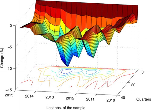
We measure time variation in the monetary policy transmission using 32 quarters rolling window regressions. Note, however, that we estimate the euro area VAR using the whole sample, thus keeping the external ‘assumptions’ unchanged.²⁵ The resulting impulse responses of the rolling window estimates are presented in Figures 9–11, where the dates in the figures correspond to the last date of the rolling 8 years sample.

Figure 9. Rolling window estimates of responses to a 100 bp Euribor shock.

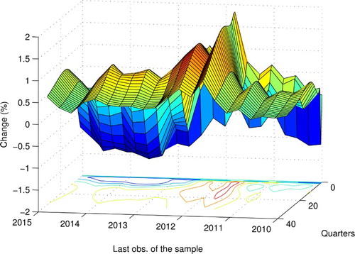
Figure 10. Rolling window estimates of responses to a 100 bp Euribor shock.

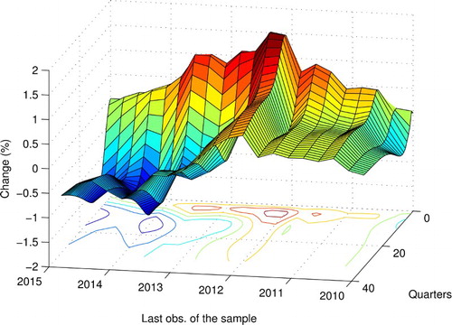
Figure 11. Rolling window estimates of responses to a 100 bp Euribor shock.

The surface plots in Figures 9–11 contain a lot of compressed information. They should be read as follows: if we sliced a graph along a selected date, we would obtain an impulse response estimated at that specific date using the sample of 8 years up to that date. In this way, a 100 bp Euribor shock effect on consumer prices (Figure 10) would have been estimated to be positive (price puzzle) in Q2 2012, while in Q4 2014 highly negative with the response trough of −1.7%.

Impulse responses in Figures 9–11, as expected, exhibit quite considerable degree of variation over time. The GDP responses seem to be the most stable of the three cases analysed: GDP always drops in the first quarters after the shock, but the effect is short-lived as the cumulative response comes back (with overshooting) towards zero. The troughs of GDP responses vary from −0.2% to −1.5% (with the trough equal to −0.9% in the last time window).

The pattern of consumer price responses is less stable over time and is also somewhat puzzling. Although it is generally agreed that contractionary monetary policy reduces prices, for samples ending up to Q3 2012 we observe mostly positive effect. One may argue that this positive effect may be due to the cost channel of monetary policy dominating other channels of transmission in the early samples; however, the model likely suffers from misspecification or omission of significant determinants present in the early samples.²⁶

Credit responses (Figure 11) are unidirectional, leading to the decrease of credit in case of contractionary shock. Note that credit is less responsive to monetary policy shock in the most recent samples with the trough of the response equal to −3.6% in the last sample. This result can be explained by less active crediting in the post-crisis period (see the graph in the lower-right corner of Figure 6).

5. Conclusions

In this work we study the effects of a euro area monetary policy shock on the Lithuanian economy. For this purpose we employ a six-dimensional SVAR model, identified using short-term zero restrictions, to analyse impulse responses of Lithuanian macro variables. Although during our sample period Lithuania was not yet part of the euro area, the domestic currency (litas) was pegged to the euro and the currency board arrangement was employed throughout the sample period. This created an environment in which Lithuanian economy showed sensitivity to the monetary policy shocks in the euro area. Therefore, our analysis is relevant in understanding the euro area monetary policy transmission in Lithuania, now that the country is within the monetary union.

We estimate the trough in the reaction of Lithuanian GDP (after a 100 bp Euribor shock) to be −0.6% (compared to −0.45% in the euro area), while the Lithuanian consumer prices reach the lowest reaction point approximately 10 quarters after the shock at −0.6% (compared to −0.2% in the euro area). The uncertainty surrounding the Lithuanian estimates, however, is also greater, resulting in statistically insignificant impulse responses of Lithuanian GDP and consumer prices.

We also find that euro area monetary policy shock has a very strong and statistically significant effect on Lithuanian credit: the trough of the response is reached three quarters after the shock at −7%. However, this result should be interpreted with a certain amount of caution, keeping in mind that during the sample period Lithuania experienced high levels of credit growth caused by the foreign capital inflows via Swedish banks operating in the Baltics, which makes it harder to separate this effect from the whole monetary effect on the real economy.

In addition to SVAR analysis, we also employed PVAR analysis using data from the three Baltic states. The estimated PVAR impulse responses for GDP and credit variables are stronger than the ones observed in the Lithuanian VAR model, though broadly within the confidence bands of Lithuanian impulse responses. The differences between impulse responses in the SVAR and PVAR analyses are hard to justify, as all three countries have had similar industry structure, hard pegs to the euro, and similar development paths. This hints that Lithuanian GDP response to a euro area monetary policy shock may be even stronger than the one estimated using the Lithuanian VAR model.

Conducting rolling regression analysis we observe quite considerable degree of variation over time in the impulse responses of PVAR model: for example, the troughs of GDP responses vary from −0.2% to −1.5%. We also observe smaller monetary policy shock impact on credit in the most recent samples, pointing to potentially weakening monetary policy transmission through crediting.

Acknowledgments

We would like to thank Lenno Uusküla, Rūta Rodzko, Sigitas Šiaudinis, Mihnea Constantinescu, Aurelijus Dabušinskas, Tomas Reichenbachas and the participants of the internal Bank of Lithuania seminars for their helpful comments and suggestions. The views expressed and the conclusions reached in this publication are those of the authors and do not necessarily represent those of the Bank of Lithuania or the Eurosystem.

Disclosure statement

No potential conflict of interest was reported by the authors.

Notes on contributors

Julius Stakėnas obtained his master in econometrics from Vilnius University, Lithuania. He is currently working as an economist in the Economics department of the Bank of Lithuania. His main interests lie in the issues of short-term forecasting: factor modelling, mixed-frequency data, forecast aggregation, global economy modelling.

Rasa Stasiukynaitė obtained her Ph.D. in Economics from Tilburg University, The Netherlands. Currently she works as an economist in the Economics department of the Bank of Lithuania. Her main interests are unconventional monetary policy transmission and policy stance assessment.

Notes

1. The assets of the financial system in Lithuania, by the end of 2014, constituted around 70% of GDP, while the same measure stood around 310% for the euro area. Source: ECB Statistical Data Warehouse and own calculations.

2. By the end of 2014, market capitalization in Lithuania was 9% of GDP, while in the euro area – around 59%. Source: ECB Statistical Data Warehouse and own calculations.

3. In 2014, the top three banks held 70% of the system's assets and over 70% of total loans, see Statistical Annex 2 of the Financial Stability Review, 2015, Lietuvos bankas.

4. Allowing the data to ‘speak’ can be perceived both as an advantage and disadvantage: without theoretical relations included in the model the outcomes might be counterintuitive, for example, a well-known ‘price puzzle’, and the results can be sensitive to various identification schemes (see, for example, Van Aarle, Garretsen, & Gobbin, 2003).

5. Estonia and Lithuania had currency boards, while Latvia – a quasi-currency board. The Estonian national currency was pegged to the DEM from 1992 and later to the euro from 1999 until the euro adoption in 2011; the Latvian currency was pegged to the euro from 2005 until the euro adoption in 2014.

6. In an earlier study, using the data for 20 industrialized countries, Georgiadis (2014) also points to financial structure, labour market rigidities and industry mix being the main determinants for differences in monetary policy transmission.

7. Note that during the period Latvia was in a fixed exchange regime.

8. In 2014 the share of Lithuanian exports to the euro area countries constituted 29% and imports — 39%. Source: Eurostat and own calculations.

9. For brevity reasons and due to the fact that every VAR(p) model can be written as VAR(1), we write the model as VAR(1). We elaborate on the lag structure later in the text.

10. For detailed data description, together with the applied data transformations, see Table A1 in Appendix 1.

11. Excluding the energy component from consumer prices helped to obtain more reasonable impulse responses to a monetary policy shock, whereas accounting for the oil price impact on HICP in the VAR model's framework proved to be a more difficult task. Nevertheless, we agree that when the Euribor equation in the euro area block is interpreted as the Taylor rule, it may be more realistic to condition the Euribor rate on the complete HICP, jointly with the commodity prices (and other indicators).

12. For the credit variable we use credit stock (nominal values). Although the data on new loans might be more relevant (it might react more to changes in the Euribor rate), due to shorter new loans data series we opted to use credit stock variable. We also tried to use credit deflated by consumer prices; however, it did not considerably change the results.

13. OLS estimates were sensitive to the inclusion of the Q1 2009 data point. We argue, that due to the various different factors (which are also difficult to account for) making this data point an outlier, it is reasonable to exclude this data point from the estimation of the Lithuanian block.

14. Credit margins are calculated as follows: where loan interest contains average interest rates on new loans (both in litas and in euros) to non-financial institutions and households; was the average 3-month interbank lending interest rate in litas.

15. In this regard our estimation strategy is reminiscent of the global VAR methodology (see Pesaran, Schuermann, & Weiner, 2004), which also uses individual country VAR estimates to build a joint model.

16. All estimations in the paper were carried out using R statistical package.

17. To illustrate this argument, we also present impulse response estimates for Lithuanian block specification in levels.

18. We use a longer sample for the euro area block because a model with levels requires longer time series. However, despite the fact that there is much more data available for the euro area block, we choose a period which is reasonable in a sense that we expect data within our chosen period to have the same structure.

19. The impulse response functions are plotted together with 68% confidence intervals. The confidence intervals are obtained using standard bootstrapping procedure with 10,000 draws.

20. Due to lack of data, we do not have the original data series for the credit margin in Latvia. However, due to largely the same main banks operating in the region (also experiencing similar economic environment), we might expect the credit margins to be very similar in the three Baltic states. Therefore, in the subsequent analysis, we will approximate the Latvian credit margin using the mean of the Lithuanian and Estonian credit margins.

21. The specific dummy variable treatment, for example, using the same dummy of Q1 2009 for all three countries, does not have a significant influence on the results.

22. Due to a fairly large T, the so-called Nickell bias should not be a cause of concern in this case. We thank the referee for pointing this out.

23. For PVAR shock identification, we applied the same identification scheme based on short-term zero restrictions as in Section 2.

24. Georgiadis (2015) points to differences in the industry mix as one of the main factors in explaining asymmetries in monetary policy transmission: economies with larger share of aggregate output accounted for by manufacturing and construction, all else being equal, exhibit larger declines in GDP in case of monetary tightening. Note that the manufacturing share in Lithuania is the largest among the three Baltic states (Figure 8), hence, the industry structure does not indicate that responses to monetary policy shock in Lithuania should be smaller than in other Baltic countries.

25. In our framework, the euro area variable responses to a 100 bp Euribor shock are the same for all rolling window regressions and are equal to the ones presented in Figure 2. Note that although this strategy helps to control for changes in monetary policy transmission in the euro area, we employed it due to the necessity to obtain reliable estimates. Panel treatment does not increase the number of observations for the EA model; therefore, it would suffer from small sample problems if it were estimated using the rolling window sample.

26. Barth and Ramey (2002) highlight the supply-side channel of monetary policy, noting that contractionary monetary policy shock may have positive effect on prices due to rising cost of firms' working capital.

Appendix 1. Data description

Table A1. Data description.

Variable	Source	Transformations	Description
GDP	Eurostat	Seasonally adjusted and adjusted by working days; Log	EA18; Gross domestic product at market prices; Chain linked volumes, index 2005=100; Eurostat code: [namq_10_gdp]
HICP	Eurostat	Seasonally adjusted using arima x12; Log	EA18: HICP excluding energy; After seasonal adjustment monthly data were aggregated to quarterly by averaging
Euribor	Bloomberg	—	3-month interbank lending interest rate in euros (average in a quarter)
GDP	Federal Reserve Bank of St. Louis	Seasonally Adjusted; Log	Real GDP; Billions of chained 2009 dollars
P	IMF	Log	All Commodity Price Index, 2005=100, includes both Fuel and Non-Fuel Price Indices
GDP	Eurostat	Seasonally adjusted and adjusted by working days; Log	Lithuanian gross domestic product at market prices; Chain linked volumes, index 2005=100; Eurostat code: [namq_10_gdp]; GDP values prior to 2005Q1 extrapolated using quarterly changes in GDP according to ESA95 ([namq_gdp_k])
Vilibor	Bank of Lithuania	—	3-month interbank lending interest rate in Lithunia in LTL (average in a quarter).
HICP	Eurostat	Seasonally adjusted using arima x12; Log	Lithuanian HICP excluding energy; After seasonal adjustment monthly data was aggregated to quarterly by averaging.
Credit	MFI balance sheet data	Log	MFI loans to non-financial corporations and households in Lithuania; Adjusted for reclassifications and technical changes.
NIIP	Eurostat		International investment position, net positions in Lithuania at the end of period
GDP	Eurostat	Seasonally adjusted and adjusted by working days; Log	Latvian gross domestic product at market prices; Eurostat code — [namq_10_gdp]; Chain linked volumes (2005), million units of national currency
HICP	Eurostat	Seasonally adjusted using arima x12; Log	Latvian HICP excluding energy; After seasonal adjustment monthly data was aggregated to quarterly by averaging.
Rigibor	Eurostat	–	3-month interbank lending interest rate in Latvia in LVL (average in a quarter); Euribor from 2014Q1
Credit	Bank of Latvia; Consolidated balance sheet of the MFIs	Log	Stock of loans to residents other than general government in Latvia; Monthly data was aggregated to quarterly by averaging
GDP	Eurostat	Seasonally adjusted and adjusted data by working days; Log	Estonian gross domestic product at market prices; Eurostat code: [namq_10_gdp]; Chain linked volumes (2005)
HICP	Eurostat	Seasonally adjusted using arima x12; Log	Estonian HICP excluding energy; After seasonal adjustment monthly data was aggregated to quarterly by averaging.
Talibor	Eurostat	–	3-month interbank lending interest rate in Estonia in EKK (average in a quarter); Euribor from 2011Q1
Credit	Eeesti Pank	Log	Loans to non-financial corporations and households (including NPISH)

Appendix 2. Additional results

Figure A1. Lithuanian variables' responses to a 100 bp Euribor shock based on the model with Lithuanian block estimated in levels.

References

- Barth III, M. J., & Ramey, V. A. (2002). The cost channel of monetary transmission. In B. S. Bernanke & K. Rogoff (Eds.), NBER Macroeconomics Annual 2001 (Vol. 16, pp. 199–256). Cambridge, MA: MIT Press.
- Bernanke, B. S., & Gertler, M. (1995). Inside the black box: The credit channel of monetary policy transmission. The Journal of Economic Perspectives, 9(4), 27–48. doi: 10.1257/jep.9.4.27
- Bitans, M., Stikuts, D., & Tillers, I., et al. (2003). Transmission of monetary shocks in Latvia (Technical report, Working paper, 2003/01). Latvijas Banka.
- Boivin, J., Kiley, M. T., & Mishkin, F. S. (2010). How has the monetary transmission mechanism evolved over time? In B. M. Friedman & M. Woodford (Eds.), Handbook of monetary economics (Vol. 3, pp. 369–422). Elsevier. Retrieved from http://econpapers.repec.org/bookchap/eeemonhes/3.htm.
- Ciccarelli, M., Maddaloni, A., & Peydró, J.-L. (2013). Heterogeneous transmission mechanism: monetary policy and financial fragility in the eurozone. Economic Policy, 28(75), 459–512. doi: 10.1111/1468-0327.12015
- Elbourne, A., & de Haan, J. (2009). Modeling monetary policy transmission in acceding countries: Vector autoregression versus structural vector autoregression. Emerging Markets Finance and Trade, 45(2), 4–20. doi: 10.2753/REE1540-496X450201
- Errit, G., & Uusküla, L. (2014). Euro area monetary policy transmission in Estonia. Baltic Journal of Economics, 14(1–2), 55–77. doi: 10.1080/1406099X.2014.980113
- Georgiadis, G. (2014). Towards an explanation of cross-country asymmetries in monetary transmission. Journal of Macroeconomics, 39, 66–84. doi: 10.1016/j.jmacro.2013.10.003
- Georgiadis, G. (2015). Examining asymmetries in the transmission of monetary policy in the Euro area: Evidence from a mixed cross-section global VAR model. European Economic Review, 75, 195–215. doi: 10.1016/j.euroecorev.2014.12.007
- Havranek, T., & Rusnák, M. (2013). Transmission lags of monetary policy: A meta-analysis. International Journal of Central Banking, 9(4), 39–75.
- Marcellino, M. (2004). The Euro area and the acceding countries. Technical report.
- Minea, A., & Rault, C. (2009). Some new insights into monetary transmission mechanism in Bulgaria. Journal of Economic Integration, 24(3), 563–595. doi: 10.11130/jei.2009.24.3.563
- Peersman, G., & Smets, F. (2001). The monetary transmission mechanism in the euro area: More evidence from VAR analysis (Working Paper Series 0091). European Central Bank.
- Pesaran, M. H., Schuermann, T., & Weiner, S. M. (2004). Modeling regional interdependencies using a global error-correcting macroeconometric model. Journal of Business and Economic Statistics, 22(2), 129–162. doi: 10.1198/073500104000000019
- Primiceri, G. E. (2005). Time varying structural vector autoregressions and monetary policy. The Review of Economic Studies, 72(3), 821–852. doi: 10.1111/j.1467-937X.2005.00353.x
- Rusnák, M., Havranek, T., & Horváth, R. (2013). How to solve the price puzzle? A meta-analysis. Journal of Money, Credit and Banking, 45(1), 37–70. doi: 10.1111/j.1538-4616.2012.00561.x
- Uhlig, H. (2005). What are the effects of monetary policy on output? Results from an agnostic identification procedure. Journal of Monetary Economics, 52(2), 381–419. doi: 10.1016/j.jmoneco.2004.05.007
- Van Aarle, B., Garretsen, H., & Gobbin, N. (2003). Monetary and fiscal policy transmission in the Euro-area: Evidence from a structural VAR analysis. Journal of Economics and Business, 55(5), 609–638. doi: 10.1016/S0148-6195(03)00056-0
- Vetlov, I. (2004). Monetary transmission mechanism in Lithuania. In D. G. Mayes (Ed.), The monetary transmission mechanism in Baltic States (pp. 61–107). Tallinn: Bank of Estonia.