Measurement and decomposition of Lithuania's income inequality

ABSTRACT

Even though Lithuania’s household income inequality is among the highest in the European Union (EU), little empirical work has been carried out to explain such disparities. We investigate it using the EU Statistics on Income and Living Conditions sample microdata. We confirm that income inequality in Lithuania is high compared to the EU average. Our decompositions reveal that the number of employed household members in Lithuania’s households affects income inequality more as compared to the EU. It is related to a larger labour income, and self-employment income, in particular, contribution to inequality in Lithuania. Moreover, taxes, social contributions, and transfers reduce income inequality in Lithuania less than in the EU. Specifically, income taxes and social contributions are less progressive while transfers constitute a smaller share of income in Lithuania than in the EU. Income taxes and social contributions are effectively regressive for the self-employed in Lithuania.

KEYWORDS:

• Income inequality
• factor decomposition
• subgroup decomposition
• Lithuania
• European Union
• Kakwani

JEL CLASSIFICATION:

• D31

1. Introduction

Income inequality in Lithuania has been one of the largest in the EU and is still growing. Specifically, the Gini coefficient of equivalised disposable income, a common measure of inequality, stood at 36.9% in 2018 for Lithuania (Eurostat, 2020). This was the second-largest Gini coefficient among the surveyed EU countries, second to Bulgaria, and exceeded the EU average income inequality by over 6 Gini points. Additionally, income inequality in Lithuania has increased by 5 Gini points since 2012. All this happened in the context of more general concern over rising income inequality within major countries (Atkinson & Piketty, 2010; OECD, 2011, 2015a, 2015b) and increasing empirical evidence that income inequality may hinder economic growth (Aghion et al., 1999; Cingano, 2014; Grigoli & Robles, 2017; Ostry & Berg, 2011; Ostry et al., 2014). The size and dynamics of income inequality in Lithuania along with warnings about its possible negative consequences encouraged political and economic debate in Lithuania. There was an interest to re-examine whether income inequality in Lithuania is indeed one of the largest within the EU, what contributes to income inequality, and what policy could be efficient at reducing it. This study focuses on these questions: how confident are we in claiming that Lithuania's income inequality is high, what factors lay behind such inequality and how much can redistribution of direct taxes and public transfers reduce income inequality.

We first analysed the extent to which income inequality is high. Even though the Gini of equivilised income does suggest this, a high Gini is not sufficient for such a claim. Besides the issue of estimating standard errors and testing for different equivalent scales, which can also change the ranking of countries according to income inequality (Buhmann et al., 1988), the Gini index itself is subject to criticism. This is because the Gini index, just like any summary inequality measure, entails social judgements on the undesirability of inequality (Atkinson, 1970). Specifically, the Gini is more sensitive to inequalities in the middle of the distribution rather than the tails. This is not necessarily a desirable property, especially for Lithuania, where the highest level of inequality was found in the tails (IMF, 2016).

For this reason, we employed several statistical tests to examine whether we can claim that equivalised income inequality in Lithuania is one of the highest across the EU. First, we have evaluated the sampling errors to verify that conclusions from the sample data do not contradict the actual situation. Rao et al. (1992) bootstrapped standard errors based on survey design information reconstructed according to Goedemé (2013) and Zardo and Goedemé (2016) allow to estimate the likely biases. Second, we have adjusted household income by alternative equivalence scales. We use the OECD-modified equivalence scale and the square root equivalence scale. Third, we have calculated inequality with other summary measures, thereby explicitly focusing on different segments of the distribution rather than the middle. We have estimated inequality using alternative measures to the Gini index: the Atkinson index and the Generalized entropy index as in Jenkins (2017) with standard inequality preference parameter values. We found that income inequality is statistically larger than the income inequality in other countries regardless of the equivalence scale or the summary measure used. This also strengthens the following analysis which is based on the Gini index.

Next, we have investigated why equivalised income inequality is higher compared to other countries using univariate factor and subgroup decompositions that decompose inequality into parts. These decompositions are purely statistical: they do not incorporate agent responses to any covariate. Nevertheless, these decompositions help identify the households amongst which inequality is acute and suggest which aspects should be looked into deeper.

Factor component decomposition decomposes inequality measure by disaggregating it into mutually exclusive and exhaustive income components, for example, labour and capital income. Two versions of this method are well known: the natural decomposition as in Shorrocks (1982) that focuses on the decomposition of the variance and the Lerman and Yitzhaki (1985) decomposition that is used to decompose the Gini coefficient. We use the latter method, as the Gini is a more conventional index of inequality. This method was used by, for example, Garner and Terrell (1998) to examine income inequality in Slovakia and Czechia in the early transition period.

Subgroup decomposition decomposes inequality measures within and between mutually exclusive and exhaustive subgroups, for example, inequality between males and females and inequality amongst males and amongst females. There are many ways to decompose subgroups as illustrated in Cowell (2011) and Yitzhaki and Lerman (1991). We apply the Yitzhaki and Lerman (1991) method to decompose the Gini in a way that is closer to the chosen factor decomposition technique.

From the decompositions, we see that labour income inequality is much higher in Lithuania than elsewhere in Europe. Additionally, in line with previous findings (e.g. IMF, 2016), the tax and public transfers system plays less of a redistributive role in Lithuania than in other countries. To understand why, we looked into marginal effects: how does a 1% change in tax and transfers affect income inequality. We also looked into redistributive effects: how much do taxes and transfers reduce inequality according to Kakwani (1977). Finally, we decompose the redistributive effect into the progressivity index and the average rate of tax and public transfers and compare this with that of the EU. This lets us calculate how much can inequality be reduced due to a change in progressivity and average tax and public transfer rates.

Overall, our results suggest that equivalised income inequality in Lithuania is one of the highest in the EU and this finding is robust to various statistical tests. The decompositions reveal large inequalities between and within many groups of households in Lithuania. The largest inequalities lie between the employed and the rest of the population, and this kind of inequality has been rising over time. Inequalities within the unemployed and those working in the agricultural sector are particularly distinct. The factor decomposition shows that labour income, especially self-employment income, is more unequally distributed in Lithuania than elsewhere. Public transfers and taxes seem to reduce income inequality in Lithuania less than in other countries. This is because taxes and public transfers in Lithuania are less progressive and the tax and public transfer rates are lower than in the EU. Income taxes and social contributions are effectively regressive for the self-employed in Lithuania unlike in the EU. It is found that to reduce income inequality in Lithuania via redistribution, the focus should be placed on increasing the progressivity of taxes and average public transfer rates.

The paper is structured as follows: in Section 2, we give definitions of income and describe the data set used throughout the empirical investigation. The other three sections answer three research questions, each using its methodology and provide comments on the results. The final section concludes.

2. Definitions and data on income

We focus on equivalised disposable income inequality. Let us explain each term in more detail. Income is defined as a yearly disposable income. To get the disposable income we subtract taxes and social contributions from gross income. We include the social contributions of the employee and employer, as we see both of them affecting the demand for labour. In addition, a new law in 2019 requested employees to pay the majority of employees' social contributions (see SODRA, 2020). Gross income is the sum of market income (labour income with social insurance contributions and capital income) and transfers (both private and public). In cases when we refer to public transfers to analyse redistribution, we add private transfers to the definition of market income. The unit of observation is a household. This assumes that household members share their income and make joint decisions. To adjust for household size, an equivalence scale is used.

Focusing on equivalised income rather than individual income affects the results and this should be briefly justified. Research literature suggests that individuals make economic decisions taking themselves as well as their household members into consideration (see, among others, Vogler & Pahl, 1994). For example, the income of all household members comprises a common budget constraint (Chiappori & Meghir, 2015) thereby influencing each household member's behaviour. Additionally, some transfers are only granted at a household level (e.g. social assistance transfer) making the allocation of this transfer to any specific member artificial. Nevertheless, each household member has their preferences and a typically unequal control of the household's budget with evidence suggesting that decisions taken within a household are rarely joint and more often dominated by a specific household member (Pahl, 1995). Therefore, while it is useful to look at equivalised income inequality to get a first idea of how unequally income is distributed within society, specific questions require looking into inequality within a household (for example, when determining how child transfers should be allocated if mothers are more likely to spend on children rather than fathers).

The data on income and covariates come from the yearly European Union Statistics on Income and Living Conditions (EU-SILC) instrument running since 2004. The data are compiled from a mixture of the survey and administrative sources. Each year around 5 thousand Lithuanian households with around 10 thousand persons over 16 years old who agree to share information on their income are included. The exact number of households and persons recorded in Lithuania and other countries in 2015 is shown in Table 1. Most of these persons provided all information on income, as can be seen from column 5 titled ‘Observations’. As all EU member states collect data using the same methodology, we can compare the inequality in Lithuania with that of other EU countries.

Table 1. EU-SILC summary statistics for 2015 income reference year.

Country	Country	Households	Household members	Observations	Average income	Median income	Gini
code	name	(thousands)	(thousands)	(thousands)	(thousand euro)	(thousand euro)	(percent)
1	2	3	4	5	6	7	8
AT	Austria	6	10.8	10.8	26.1	23.7	27.2
BE	Belgium	5.9	11.1	11.1	24.3	22.3	26.3
BG	Bulgaria	7.3	15.6	15.5	3.9	3.2	37.7
CH	Switzerland	7.8	14.9	14.9	50.9	44.3	29.4
CY	Cyprus	4.2	9.4	9.4	16.9	14	32.1
CZ	Czech Republic	8.5	16.2	16.2	8.8	7.8	25.1
DE	Germany	13.3	23.3	23.1	23.9	21.2	29.8
DK	Denmark	6.3	11.8	11.8	32.1	28.7	27.7
EE	Estonia	6	12.5	12.5	10.1	8.6	32.7
EL	Greece	18.3	38	37.9	8.7	7.5	34.3
ES	Spain	14.2	30.7	30.7	15.8	13.7	34.5
FI	Finland	10.6	20.7	20.7	26.4	23.6	25.4
FR	France	11.5	21.3	21.3	25.3	21.7	29.2
HR	Croatia	7.6	17	17	6.3	5.7	29.8
HU	Hungary	8	15.9	15.8	5.4	4.8	28.2
IE	Ireland	5.2	10.2	10.2	25.5	22.4	29.5
IT	Italy	21.3	41.5	41.5	18.3	16.2	33.1
LT	Lithuania	4.8	9.6	9.6	7	5.6	37.0
LU	Luxembourg	3.8	8.2	8.2	39.8	34.4	31.5
LV	Latvia	6	11.6	11.6	7.5	6.4	34.5
NL	Netherlands	12.7	24.1	24.1	25.4	22.7	26.9
NO	Norway	6.9	13.6	13.6	43	39.6	24.9
PL	Poland	12	27.1	27.1	6.7	5.9	29.8
PT	Portugal	10.6	22.7	22.7	10.6	8.8	33.9
RO	Romania	7.4	15.8	15.7	2.7	2.4	34.8
RS	Serbia	5.6	15.1	15.1	3	2.6	38.6
SE	Sweden	5.8	11.2	11.2	27.3	25.2	27.6
SI	Slovenia	8.6	21.9	21.9	13.2	12.3	24.3
SK	Slovakia	5.7	14.1	14.1	7.4	7	24.3
UK	United Kingdom	9.7	17.8	17.6	24.6	21.1	31.5

Notes: The variables ‘Households’ and ‘Household members’ are the unique number of households and household members in the data set. The variable ‘Observations’ refers to those household members for whom all income data is available. Columns 6–8 refer to the average, median and the Gini coefficient of the population estimate of equivalized household disposable income.

While the data is explained by Eurostat (2018c), several features are mentioned here. The survey captures household income and, therefore, certain income components are available for the household rather than the individual level. Therefore, the income of all household members is summed up and allocated to each household member. While most covariates are recorded at the time of the interview, income is recorded for a previous year (the reference year). In this paper, all years represent reference years. While the EU-SILC has a large survey component, some countries make use of register (administrative) data and are referred to as register countries. In 2015, the register countries included Cyprus, Denmark, Finland, Latvia, Lithuania, the Netherlands, Northern Ireland, Norway, Slovenia, Sweden, and Switzerland. Finally, survey weights are used to form conclusions on the population from the sample data. The weights are further adjusted according to Eurostat (2018b): weights of household members over 16 years old are scaled up by distributing weights of those under 16.

3. Is income inequality in Lithuania high?

First, we have examined inequality from the full data sample and then analysed subgroup inequality (inequality between- and within-subgroups) in Lithuania.

3.1. Inequality

The most popular measure of the level of inequality is the Gini coefficient. The higher the Gini, the greater the level of inequality and it stood at G=0.37 for Lithuania in 2015 (Eurostat, 2020). The Gini is represented, as in Lerman and Yitzhaki (1985), by two times the covariance between income y and the rank of income $F\left(y\right)$ divided by average income μ,(1) $G=\frac{2Cov(y,F(y\left)\right)}{\mu },$(1) which describes inequality within the entire population. Since we have sample data only, we modify (1(1) $G=\frac{2Cov(y,F(y\left)\right)}{\mu },$(1) ) to include sample weights, as shown in (A1(A1) $\hat{G}=\frac{2}{\hat{\mu }}\left(\frac{1}{\hat{N}}\sum _{i\in s}{w}_i{y}_i\hat{F}\left(y_i\right)-\frac{1}{{\hat{N}}^2}\sum _{i\in s}{w}_i{y}_i\sum _{i\in s}{w}_i\hat{F}\left(y_i\right)\right)$(A1) ) in Appendix.

Lithuania's Gini coefficient has been compared with the Gini coefficients of all countries that are included in the EU-SILC data set for 2015 in Figure 1 and with the Gini coefficients for a subset of all countries in Table 2. The subset of countries includes the Baltic States, Finland as one of the Scandinavian countries, Germany – which represents the average inequality in the EU and Slovakia, where inequality is the lowest. As in previous studies (IMF, 2016; Lazutka, 2017), income inequality in Lithuania is one is of the highest according to the EU-SILC. The estimated confidence intervals (Figure 1) and standard errors (Table 2) indicate that this is statistically significant. For example, the Gini in Lithuania is about 7 Gini points higher than in Germany. The latter also happens to be the median in terms of inequality within the whole EU-SILC sample of countries.

Figure 1. The Gini coefficients of equivalised disposable income in all EU-SILC countries. Household disposable income is equivalised by the OECD-modified scale. Confidence intervals are estimated by using Rao et al. (1992) bootstrap methodology. Information on survey design is provided by Goedemé (2013) and Zardo and Goedemé (2016).

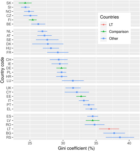
Table 2. Income inequality measures under different equivalence scales.

Country	Equivalence scale	G(2)	G(1.5)	G(4)	GEI(0)	GEI(1)	GEI(2)	Atk(1)	Atk(0.1)
DE	OECD	29.764	19.602	46.279	0.157	0.158	0.220	0.146	0.016
		(0.373)	(0.318)	(0.388)	(0.004)	(0.006)	(0.016)	(0.004)	(0.001)
EE	OECD	32.738	21.096	51.419	0.192	0.171	0.188	0.175	0.017
		(0.358)	(0.256)	(0.463)	(0.006)	(0.004)	(0.005)	(0.005)	(0.000)
FI	OECD	25.416	16.897	40.216	0.112	0.116	0.150	0.106	0.011
		(0.283)	(0.236)	(0.340)	(0.003)	(0.004)	(0.009)	(0.003)	(0.000)
LT	OECD	36.957	24.644	55.797	0.254	0.233	0.306	0.224	0.023
		(0.755)	(0.609)	(0.801)	(0.012)	(0.011)	(0.022)	(0.009)	(0.001)
LV	OECD	34.479	22.756	53.403	0.217	0.202	0.255	0.195	0.020
		(0.511)	(0.432)	(0.563)	(0.007)	(0.008)	(0.019)	(0.006)	(0.001)
Median	OECD	29.764	19.719	46.279	0.158	0.163	0.228	0.146	0.016
		(0.373)	(0.538)	(0.388)	(0.008)	(0.011)	(0.039)	(0.006)	(0.001)
SK	OECD	24.277	15.624	40.310	0.115	0.106	0.136	0.109	0.011
		(0.482)	(0.383)	(0.682)	(0.006)	(0.007)	(0.022)	(0.005)	(0.001)
DE	Sqr. rt	30.224	19.873	47.169	0.163	0.162	0.223	0.150	0.016
		(0.379)	(0.324)	(0.389)	(0.004)	(0.006)	(0.016)	(0.004)	(0.001)
EE	Sqr. rt	33.158	21.305	52.399	0.199	0.175	0.190	0.180	0.017
		(0.354)	(0.253)	(0.451)	(0.006)	(0.004)	(0.005)	(0.005)	(0.000)
FI	Sqr. rt	25.918	17.202	41.213	0.117	0.120	0.155	0.110	0.012
		(0.288)	(0.240)	(0.347)	(0.003)	(0.004)	(0.009)	(0.003)	(0.000)
LT	Sqr. rt	37.383	24.854	56.684	0.261	0.237	0.307	0.230	0.023
		(0.763)	(0.625)	(0.790)	(0.012)	(0.011)	(0.023)	(0.009)	(0.001)
LV	Sqr. rt	35.039	23.063	54.513	0.226	0.207	0.259	0.202	0.021
		(0.521)	(0.447)	(0.553)	(0.007)	(0.008)	(0.021)	(0.006)	(0.001)
Median	Sqr. rt	29.699	19.873	47.169	0.161	0.162	0.223	0.149	0.016
		(0.662)	(0.324)	(0.389)	(0.008)	(0.006)	(0.016)	(0.007)	(0.001)
SK	Sqr. rt	25.000	16.043	41.302	0.120	0.109	0.132	0.113	0.011
		(0.447)	(0.350)	(0.622)	(0.006)	(0.006)	(0.016)	(0.005)	(0.001)

Notes: Table contains inequality measures for the median country (from all EU countries) and selected countries for each equivalence scale. $G\left(v\right)$ represents the Gini index with values v=2,1.5,4 of parameter of inequality aversion, $GEI\left(a\right)$ stands for the General entrhopy index, and $Atk\left(b\right)$ is the Atkinson index, where b=1,0.1 and a=0,1,2 represents the degree of inequality aversion. Bootstrapped standard errors are presented in the parenthesis.

Although Table 2 focuses on fewer countries, it provides more statistics on inequality than Figure 1. In Figure 1, household disposable income is equivalised by the OECD-modified equivalence scale. In Table 2, two different scales are used: the OECD-modified scale and the square root equivalence scale. The square root scale increases the Gini for Lithuania by 0.3 points, yet remains with the highest level of income inequality among all countries and 7 Gini points higher than the median country.

Furthermore, in Table 2, the generalized Gini coefficient, $G\left(v\right)$ (Yitzhaki, 1983), where parameter v represents inequality aversion. This inequality parameter represents the dissatisfaction expressed towards inequality. With this parameter we can model different societal preferences. The value v=2 gives the standard Gini, v between 1 and 2 represent lower inequality dissatisfaction and v>2 indicates higher dissatisfaction. The measurement $G\left(1.5\right)$ results in lower Gini values in all countries for both equivalence scales (i.e. inequality is not as ‘bad’). Additionally, the difference between the Gini in Lithuania and the median country shrinks to 5 Gini points for both scales. Nevertheless, inequality in Lithuania remains significantly the highest out of the sample of six countries. Setting v=4 increases the Gini index, but for Lithuania it remains the highest among the selected countries.

Finally, the Gini is compared with other measures of inequality. Other prominent measures include the Atkinson index (Atk) and General entropy index (GEI), see Das and Parikh (1982), Cowell (2000) and Plat (2012). Both of these measures show that the higher the value, the greater the inequality. Both indexes also feature inequality aversion parameters. In the Atkinson index, a parameter value close to zero means indifference about inequality, while higher values show that people dislike it. In contrast, high GEI parameter values mean that people are indifferent about inequality. In all cases, inequality in Lithuania remained significantly the highest.

3.2. Subgroup inequality

The previous subsection has shown that inequality in Lithuania is large when compared to EU countries. Next, we will consider inequality between and within population subgroups, for example, between males and females and amongst males and females. Then we will estimate stratification – the extent to which income of one group overlaps income of other groups.

Continuing the discussion started in Section 2, the interpretation of a subgroup may not be straightforward, as we are dealing with equivalised income instead of individual income, but can be explained with the help of an example. Imagine a household composed of one male and one female. Then, comparing household income (i.e. adding up household members' income and allocating the summed household income to each member) implies no income inequality between the male and the female in that household. However, this is only true if all households have the same number of males and females. Some households are consisting of more males, while others have a higher number of female members. If males tend to earn more than females, households with more males will earn higher equivalised household income than equivalised households with more females. In aggregate, this will lead to inequalities between the subgroups. Inequality between this group should be interpreted as ‘inequality between male and female-dominated households’. This way, we can combine information on household income and the composition with individual characteristics. Of course, there could be other variables that are also correlated. For example, females tend to live longer and are therefore more likely to be retired and hence receive lower income. However, this approach abstracts from other variables.

The methodology used to estimate inequality between subgroups is similar to the one used by IMF (2016) and is based on Eurostat (2018a). The methodology for estimating inequality within subgroups and stratification are adapted from Yitzhaki and Lerman (1991). Additionally, the technique proposed by Yitzhaki and Lerman (1991) is used to decompose total inequality into between, within and stratification terms to see which of them contributes most to inequality.

Inequality between subgroupsInequality between subgroups refers to measured inequality between households grouped under certain criteria. For example, households can be grouped by ‘Sex’ into two subgroups l=1 and l=2: ‘Males’ and ‘Females’. To estimate between subgroup inequality, we first estimate the weighted average income of a subgroup ${\hat{m}}^{\left(l\right)}$ and then divide by the average weighted income of all subgroups $\hat{m}$, see (A3(A3) ${\hat{N}}_l=\sum _{j\in s_l}{w}_j,{\hat{P}}_l=\frac{{\hat{N}}_l}{\hat{N}},\hat{m}=\frac{1}{\hat{N}}\sum _{j\in s}{w}_j{y}_j,{\hat{m}}^{\left(l\right)}=\frac{1}{{\hat{N}}_l}\sum _{j\in s_l}{w}_j{y}_j,{\hat{F}}^{\left(l\right)}=\frac{1}{{\hat{N}}_l}\sum _{i\in s_l}{w}_i\hat{F}\left(y_i\right),$(A3) ) in Appendix 1, to get an income ratio ${\hat{m}}^{\left(l\right)}/\hat{m}$. We then compare the ratio with that of the EU, namely of its member states that joined the EU before 2004 (old EU states), and with those Member States that joined it after 2004 (new EU states). Our method is similar to that used in the IMF (2016), but has several differences: the IMF (2016) analyse weighted income decile ratios while we compare weighted average income ratios. The IMF (2016) compares Lithuania to the EU, while we additionally compare it to new and old EU states to control for the development of countries. Finally, we have more grouping criteria (a total of nine) and estimate standard errors.

Our findings are in line with those of IMF (2016), which also reviews between-subgroup inequality in Lithuania. The IMF (2016) reveals large inequalities between the top and the bottom income deciles, between the employed and the unemployed and non-labour market participants, between the elderly and other age subgroups, as well as between educated and less educated households subgroups, i.e. these ratios are much higher in Lithuania than in the entire EU.

In addition to these findings, the results presented in Table 3 allow adding the following points:

Table 3. Ratios of average subgroup incomes in 2015.

Grouping	Subgroup	EU	EU new	EU old	LT
activity status	employed	113.2 (0.5) [25.5]	115.4 (0.9) [9.8]	112.6 (0.6) [15.5]	123.2 (1.3) [5.2]
activity status	unemployed	61.0 (1.3) [3.3]	59.5 (1.9) [1.2]	61.3 (1.6) [2.0]	54.0 (3.6) [0.6]
activity status	retired	97.3 (1.0) [9.5]	95.2 (1.3) [4.2]	97.9 (1.2) [5.6]	71.1 (1.7) [2.0]
activity status	study	85.5 (1.6) [3.5]	88.4 (2.4) [1.3]	84.8 (1.8) [2.2]	86.8 (3.2) [0.7]
activity status	other	77.4 (1.3) [5.7]	70.5 (1.9) [2.2]	79.2 (1.6) [3.5]	68.9 (3.1) [1.0]
nr working	0	78.3 (0.9) [12.8]	75.1 (1.2) [4.6]	79.0 (1.0) [8.0]	53.3 (1.6) [2.4]
nr working	1	93.4 (0.9) [15.1]	93.6 (1.6) [5.8]	93.3 (1.0) [9.2]	94.1 (2.6) [3.1]
nr working	2	119.3 (0.9) [16.7]	117.8 (1.4) [6.7]	119.7 (1.0) [10.1]	131.4 (2.8) [3.3]
nr working	3	116.9 (2.3) [2.5]	115.6 (4.1) [1.5]	117.5 (2.7) [1.3]	130.5 (4.8) [0.6]
nr working	4	124.3 (4.2) [0.6]	124.0 (5.3) [0.4]	124.5 (6.0) [0.3]	124.9 (8.6) [0.2]
main income	employment	108.7 (0.6) [24.1]	112.2 (0.9) [11.7]	107.4 (0.8) [13.6]	111.5 (1.4) [6.1]
main income	self-employment	106.3 (3.2) [3.4]	84.3 (3.2) [1.7]	114.8 (4.2) [1.9]	174.9 (10.7) [0.7]
main income	other	88.7 (0.6) [20.4]	79.3 (1.6) [5.6]	90.4 (0.7) [13.4]	57.6 (1.6) [2.8]
occupation	basic level	74.6 (1.3) [4.5]	78.1 (4.1) [1.9]	73.7 (1.2) [2.7]	69.6 (2.5) [1.4]
occupation	mid-level	90.0 (0.6) [21.0]	91.9 (0.8) [9.6]	89.3 (0.7) [12.2]	88.7 (1.7) [4.1]
occupation	technicians, associates	112.9 (1.3) [6.0]	118.7 (2.1) [1.6]	111.9 (1.4) [3.9]	117.8 (4.6) [0.6]
occupation	professionals	139.1 (1.8) [7.3]	145.8 (2.6) [2.4]	137.7 (2.1) [4.6]	129.1 (3.1) [1.9]
occupation	managers	137.9 (3.3) [2.3]	153.0 (5.5) [0.8]	134.7 (3.8) [1.5]	162.7 (11.6) [0.6]
sector	agriculture	74.2 (2.6) [1.0]	66.4 (2.5) [1.0]	83.4 (4.7) [0.3]	99.5 (6.7) [0.3]
sector	industry	115.6 (1.9) [3.4]	116.2 (2.3) [2.0]	115.3 (2.5) [1.8]	113.9 (3.8) [0.8]
sector	IT, finance, RE, admin	134.4 (2.7) [3.4]	158.2 (7.9) [0.9]	130.6 (2.8) [2.2]	157.2 (10.9) [0.6]
sector	public admin, education, health	118.0 (1.3) [5.8]	127.1 (2.3) [1.7]	116.4 (1.5) [3.7]	124.6 (3.2) [1.1]
sector	other services	100.2 (1.1) [7.6]	109.5 (1.8) [3.0]	97.8 (1.3) [4.6]	119.3 (2.8) [1.8]
age bracket	under 19	83.8 (2.0) [1.8]	82.4 (3.5) [0.7]	84.2 (2.3) [1.1]	83.6 (4.1) [0.4]
age bracket	19–29	91.3 (1.3) [6.9]	95.5 (1.9) [3.0]	90.0 (1.5) [4.1]	104.2 (3.8) [1.7]
age bracket	30–64	103.9 (0.4) [30.1]	104.0 (0.6) [12.0]	103.9 (0.5) [18.1]	107.7 (1.2) [5.7]
age bracket	65+	96.9 (1.1) [9.1]	93.5 (1.4) [3.3]	97.7 (1.3) [5.6]	76.2 (1.9) [1.9]
dependents	0	105.2 (0.6) [24.5]	105.4 (1.1) [8.9]	105.2 (0.7) [15.1]	101.0 (1.8) [4.8]
dependents	1	102.6 (1.3) [9.2]	107.0 (1.9) [4.3]	101.1 (1.6) [5.3]	106.7 (3.2) [2.1]
dependents	2	94.2 (1.1) [9.7]	93.2 (1.8) [3.9]	94.5 (1.3) [5.8]	102.4 (4.8) [2.0]
dependents	3	82.7 (2.1) [3.2]	80.7 (3.7) [1.2]	83.2 (2.5) [2.0]	73.9 (6.9) [0.5]
dependents	4	73.0 (4.5) [0.8]	60.9 (6.2) [0.3]	75.9 (5.3) [0.5]	55.6 (5.5) [0.1]
dependents	5	50.9 (4.5) [0.4]	40.0 (3.5) [0.3]	58.7 (6.1) [0.2]	47.1 (11.8) [0.1]
education	up to secondary	87.8 (0.4) [32.4]	87.9 (0.6) [14.1]	87.8 (0.5) [19.0]	78.2 (1.5) [4.6]
education	post-secondary	103.0 (2.5) [1.5]	107.3 (3.9) [0.6]	101.7 (3.1) [0.9]	92.7 (2.3) [1.9]
education	tertiary education	129.6 (1.0) [13.4]	142.1 (2.0) [3.9]	127.3 (1.2) [8.6]	138.1 (2.8) [3.0]
sex	male	102.2 (0.5) [22.7]	102.8 (0.9) [9.0]	102.1 (0.7) [13.7]	104.5 (0.8) [4.3]
sex	female	98.0 (0.5) [25.2]	97.4 (0.8) [10.0]	98.1 (0.6) [15.2]	96.4 (0.6) [5.3]

Notes: Ratios are defined as weighted average income of a subgroup divided by weighted average income of all subgroups within that grouping. Bootstrapped standard errors are in the parenthesis. Number of observations in thousands in brackets.

• Differences of ratios are significant between many subgroups in Lithuania. The subgroups include those grouped according to the IMF (2016) criteria (activity status, age bracket, number of dependants, education) as well as ratios in other subgroups. For example, we split households based on the main income source. Those who receive largely self-employment income tend, on average, to have more disposable income than those who work as employees or others – a trend not observed in the EU as a whole. Significant inequality also exists between subgroups grouped by the number of people working in the household (nr working) and the sector where one works (sector).

• Ratios between the majority of the nine subgroups are also significantly different from the ratios between their EU counterparts. Besides the subgroups in the IMF (2016) (those grouped by activity status, age bracket, education), the self-employed in Lithuania on average earn proportionally more than their EU counterparts. Additionally, those who work in the information technologies, finance, real estate, and administration sector (IT, finance, RE, admin) earn, on average, relatively more income in Lithuania than one would in the EU.

• There are some groups between which inequality in Lithuania is smaller as compared to the EU. For example, those working within the agricultural sector are relatively better off in Lithuania compared to the EU. Additionally, income ratios in Lithuania are more similar to those in the new EU states. In particular, those who are under 19 years old have very similar relative incomes both in Lithuania and in the new EU states.

In general, ratios between subgroups are largely persistent and slightly widening since 2010. This can be seen in Table 4 which shows the ratio dynamics in Lithuania. For example, there was a slowly widening gap between the employed and the retired. This could be explained by rising market incomes due to a recovering economy that benefited the employed while statutory pensions, the main source of income for the retired, did not increase in the period due to budget consolidation (Černiauskas et al., 2020). Once the recovery began, wages in the private sector started rising, especially IT, finance, RE, admin sector, while the government started raising public sector wages (Public admin, education, health) much later. This could also explain the rising ratio difference between the two sectors.

Table 4. Ratios of average subgroup incomes in Lithunia.

Grouping	Subgroup	2006	2010	2015
activity status	employed	120.2 (0.9) [6.2]	122.1 (1.1) [5.4]	123.2 (1.3) [5.2]
activity status	unemployed	51.1 (2.7) [0.4]	57.7 (2.3) [1.1]	54.0 (3.6) [0.6]
activity status	retired	70.4 (1.2) [2.0]	86.4 (1.3) [2.3]	71.1 (1.7) [2.0]
activity status	study	89.1 (2.2) [1.1]	86.2 (2.3) [1.1]	86.8 (3.2) [0.7]
activity status	other	70.7 (2.2) [1.1]	74.3 (1.9) [1.0]	68.9 (3.1) [1.0]
nr working	0	51.4 (1.2) [2.1]	66.2 (1.3) [3.1]	53.3 (1.6) [2.4]
nr working	1	86.5 (1.8) [3.0]	89.7 (1.8) [3.4]	94.1 (2.6) [3.1]
nr working	2	122.0 (1.6) [4.7]	128.9 (2.1) [3.6]	131.4 (2.8) [3.3]
nr working	3	137.5 (5.6) [0.8]	144.7 (6.8) [0.7]	130.5 (4.8) [0.6]
nr working	4	138.7 (11.2) [0.2]	122.2 (11.5) [0.2]	124.9 (8.6) [0.2]
main income	employment	114.9 (0.9) [7.5]	115.3 (1.1) [6.7]	111.5 (1.4) [6.1]
main income	self-employment	106.1 (5.6) [0.6]	127.1 (10.8) [0.4]	174.9 (10.7) [0.7]
main income	other	59.0 (1.4) [2.8]	71.0 (1.2) [3.9]	57.6 (1.6) [2.8]
occupation	basic level	72.1 (1.8) [1.6]	72.6 (1.7) [1.5]	69.6 (2.5) [1.4]
occupation	mid-level	90.0 (1.1) [5.1]	87.6 (1.1) [4.8]	88.7 (1.7) [4.1]
occupation	technicians, associates	120.0 (4.3) [0.7]	119.3 (3.8) [0.7]	117.8 (4.6) [0.6]
occupation	professionals	146.4 (3.4) [1.5]	138.9 (2.8) [1.9]	129.1 (3.1) [1.9]
occupation	managers	149.9 (4.6) [0.7]	146.0 (4.6) [0.7]	162.7 (11.6) [0.6]
sector	agriculture	85.1 (5.2) [0.5]	90.9 (5.9) [0.4]	99.5 (6.7) [0.3]
sector	industry	109.9 (2.6) [1.1]	113.8 (3.9) [0.9]	113.9 (3.8) [0.8]
sector	IT, finance, RE, admin	168.2 (8.0) [0.2]	137.2 (4.9) [0.5]	157.2 (10.9) [0.6]
sector	public admin, education, health	131.2 (2.7) [1.4]	138.1 (3.1) [1.3]	124.6 (3.2) [1.1]
sector	other services	117.0 (1.9) [2.2]	111.6 (2.2) [1.8]	119.3 (2.8) [1.8]
age bracket	under 19	82.0 (2.6) [0.6]	80.3 (2.8) [0.6]	83.6 (4.1) [0.4]
age bracket	19–29	111.2 (2.9) [2.2]	101.7 (2.6) [2.0]	104.2 (3.8) [1.7]
age bracket	30–64	105.1 (0.9) [6.4]	104.3 (0.8) [6.4]	107.7 (1.2) [5.7]
age bracket	65+	73.6 (1.4) [1.8]	90.4 (1.6) [2.0]	76.2 (1.9) [1.9]
dependents	0	104.0 (1.4) [5.3]	102.7 (1.4) [4.9]	101.0 (1.8) [4.8]
dependents	1	106.0 (2.3) [2.9]	102.9 (2.2) [2.8]	106.7 (3.2) [2.1]
dependents	2	95.0 (2.8) [2.0]	99.0 (3.3) [2.3]	102.4 (4.8) [2.0]
dependents	3	72.5 (4.6) [0.5]	81.8 (6.5) [0.7]	73.9 (6.9) [0.5]
dependents	4	45.7 (10.5) [0.1]	66.8 (10.1) [0.2]	55.6 (5.5) [0.1]
dependents	5	35.9 (6.4) [0.1]	95.5 (16.1) [0.1]	47.1 (11.8) [0.1]
education	up to secondary	81.5 (0.9) [5.8]	81.7 (1.0) [6.0]	78.2 (1.5) [4.6]
education	post-secondary	95.9 (1.6) [2.4]	96.1 (2.0) [2.1]	92.7 (2.3) [1.9]
education	tertiary education	148.5 (2.4) [2.5]	140.6 (2.2) [2.9]	138.1 (2.8) [3.0]
sex	male	104.9 (0.6) [4.9]	102.9 (0.7) [4.9]	104.5 (0.8) [4.3]
sex	female	96.0 (0.5) [6.0]	97.6 (0.5) [6.1]	96.4 (0.6) [5.3]

Notes: Ratios are defined as weighted average income of a subgroup divided by weighted average income of all subgroups within that grouping. Bootstrapped standard errors are in the parenthesis. Number of observations in thousands in brackets.

Inequality within subgroupsInequality exists within subgroups in Lithuania. A common way to measure it is to calculate inequality measures for subgroup income as is done for total income (see ${\hat{G}}_l$ in Formula (A4(A4) $\hat{G}=\underset{\mathrm{W}\mathrm{i}\mathrm{t}\mathrm{h}\mathrm{i}\mathrm{n}}{\underbrace{\sum _{l=1}^L{\hat{S}}_l{\hat{G}}_l}}+\underset{\mathrm{S}\mathrm{t}\mathrm{r}\mathrm{a}\mathrm{t}\mathrm{i}\mathrm{f}\mathrm{i}\mathrm{c}\mathrm{a}\mathrm{t}\mathrm{i}\mathrm{o}\mathrm{n}}{\underbrace{\sum _{l=1}^L{\hat{S}}_l{\hat{G}}_l{\hat{Q}}_l\left({\hat{P}}_l-1\right)}}+\underset{\mathrm{B}\mathrm{e}\mathrm{t}\mathrm{w}\mathrm{e}\mathrm{e}\mathrm{n}}{\underbrace{\frac{2\hat{c}ov(m^{\left(l\right)},F^{\left(l\right)})}{\hat{m}}}},$(A4) ) in Appendix 1). We have calculated the Gini coefficients for Lithuania's subgroups and compared them with the Gini coefficients of the EU, new and old EU states in Table 5.

• Most of the within-subgroup Gini coefficients examined in Table 5 are higher in Lithuania than in the EU. Especially large subgroup inequality exists among those working in the agricultural sector and the unemployed.

• The above-mentioned within-group inequalities are much higher in Lithuania than in the EU. Additionally, households, where the main source of income is self-employment income, are also unequal among themselves, even though similar inequality within subgroups exists in new EU states. The Gini of households with many children is relatively small and we know from the between analysis that these households earn a much lower income.

Table 5. The Gini coefficient of income of subgroups in 2015.

Grouping	Subgroup	EU	new EU states	old EU states	LT
activity status	employed	28.6 (0.4) [25.5]	29.7 (0.7) [9.8]	28.3 (0.4) [15.5]	33.0 (0.9) [5.2]
activity status	unemployed	35.1 (0.9) [3.3]	36.9 (1.3) [1.2]	34.6 (1.1) [2.0]	47.8 (2.2) [0.6]
activity status	retired	27.4 (0.5) [9.5]	25.9 (0.5) [4.2]	27.8 (0.7) [5.6]	29.6 (1.0) [2.0]
activity status	student	32.2 (0.8) [3.5]	30.1 (1.0) [1.3]	32.7 (0.9) [2.2]	35.1 (1.6) [0.7]
activity status	other	32.5 (0.8) [5.7]	31.3 (1.1) [2.2]	32.7 (1.0) [3.5]	38.0 (1.5) [1.0]
nr working	0	32.2 (0.6) [12.8]	31.1 (0.9) [4.6]	32.4 (0.6) [8.0]	31.5 (1.5) [2.4]
nr working	1	31.6 (0.6) [15.1]	32.2 (1.2) [5.8]	31.4 (0.6) [9.2]	36.4 (1.1) [3.1]
nr working	2	26.5 (0.4) [16.7]	27.2 (0.6) [6.7]	26.3 (0.5) [10.1]	31.6 (1.3) [3.3]
nr working	3	25.1 (0.9) [2.5]	27.6 (1.7) [1.5]	23.8 (1.0) [1.3]	21.0 (1.4) [0.6]
nr working	4	24.6 (1.3) [0.6]	25.2 (1.9) [0.4]	24.2 (1.8) [0.3]	17.7 (3.3) [0.2]
main income	employment	27.2 (0.3) [24.1]	27.0 (0.4) [11.7]	27.3 (0.4) [13.6]	31.3 (0.9) [6.1]
main income	self-employment	42.6 (1.3) [3.4]	39.1 (1.6) [1.7]	43.0 (1.5) [1.9]	39.7 (2.2) [0.7]
main income	other	31.9 (0.4) [20.4]	33.9 (1.3) [5.6]	31.5 (0.5) [13.4]	33.0 (1.3) [2.8]
occupation	basic level	28.7 (1.0) [4.5]	33.1 (3.5) [1.9]	27.4 (0.7) [2.7]	35.6 (1.4) [1.4]
occupation	mid-level	27.5 (0.3) [21.0]	27.5 (0.5) [9.6]	27.5 (0.4) [12.2]	34.8 (0.9) [4.1]
occupation	technicians, associates	25.2 (0.6) [6.0]	24.4 (0.7) [1.6]	25.3 (0.7) [3.9]	31.0 (1.5) [0.6]
occupation	professionals	29.2 (0.8) [7.3]	25.9 (0.8) [2.4]	29.8 (0.9) [4.6]	31.0 (0.9) [1.9]
occupation	managers	31.9 (1.1) [2.3]	30.9 (1.7) [0.8]	31.9 (1.3) [1.5]	39.6 (2.5) [0.6]
sector	agriculture	35.2 (1.7) [1.0]	35.2 (1.5) [1.0]	34.0 (2.9) [0.3]	44.5 (2.4) [0.3]
sector	industry	27.1 (0.9) [3.4]	26.4 (0.8) [2.0]	27.4 (1.2) [1.8]	30.3 (1.4) [0.8]
sector	IT, finance, RE, admin	30.8 (1.0) [3.4]	31.5 (3.2) [0.9]	30.5 (1.0) [2.2]	35.1 (2.9) [0.6]
sector	public admin, education, health	25.7 (0.5) [5.8]	25.0 (0.8) [1.7]	25.7 (0.6) [3.7]	28.7 (1.0) [1.1]
sector	other services	27.9 (0.6) [7.6]	27.0 (0.8) [3.0]	27.9 (0.7) [4.6]	32.7 (1.2) [1.8]
age bracket	under 19	31.1 (1.1) [1.8]	32.8 (1.5) [0.7]	30.6 (1.3) [1.1]	34.8 (1.9) [0.4]
age bracket	19–29	30.8 (0.7) [6.9]	31.0 (1.0) [3.0]	30.6 (0.9) [4.1]	35.8 (1.4) [1.7]
age bracket	30–64	31.1 (0.3) [30.1]	31.7 (0.6) [12.0]	31.0 (0.4) [18.1]	37.4 (0.9) [5.7]
age bracket	65+	28.4 (0.7) [9.1]	26.7 (0.5) [3.3]	28.8 (0.8) [5.6]	30.8 (1.1) [1.9]
dependents	0	31.1 (0.4) [24.5]	30.8 (0.7) [8.9]	31.1 (0.4) [15.1]	38.4 (0.8) [4.8]
dependents	1	29.9 (0.6) [9.2]	29.2 (0.8) [4.3]	30.1 (0.8) [5.3]	30.8 (1.3) [2.1]
dependents	2	28.4 (0.6) [9.7]	29.2 (1.0) [3.9]	28.1 (0.7) [5.8]	37.9 (2.3) [2.0]
dependents	3	32.2 (1.1) [3.2]	32.2 (2.1) [1.2]	32.2 (1.3) [2.0]	36.2 (3.0) [0.5]
dependents	4	30.5 (2.6) [0.8]	34.6 (3.0) [0.3]	29.1 (3.0) [0.5]	20.7 (3.9) [0.1]
dependents	5	25.8 (4.0) [0.4]	21.9 (3.9) [0.3]	23.7 (5.7) [0.2]	24.7 (9.9) [0.1]
education	up to secondary	29.0 (0.3) [32.4]	29.7 (0.6) [14.1]	28.8 (0.4) [19.0]	35.0 (0.8) [4.6]
education	post-secondary	27.8 (1.0) [1.5]	28.2 (1.3) [0.6]	27.6 (1.2) [0.9]	34.7 (1.2) [1.9]
education	tertiary education	29.6 (0.5) [13.4]	27.1 (0.6) [3.9]	30.0 (0.6) [8.6]	33.1 (1.2) [3.0]
sex	male	31.0 (0.4) [22.7]	31.1 (0.6) [9.0]	30.9 (0.4) [13.7]	37.0 (0.9) [4.3]
sex	female	30.6 (0.4) [25.2]	30.9 (0.7) [10.0]	30.5 (0.5) [15.2]	36.8 (0.8) [5.3]

Notes: Bootstrapped standard errors are provided in the parenthesis. Number of observations are shown in thousands in brackets.

Over time, inequality within subgroups increased in many subgroups. Table 6 shows that the rise has been especially strong since 2010. In particular, the Gini coefficient of the unemployed rose from 39.8 in 2004 to 47.8 in 2015. This may be in part due to unequal economic recovery, where some of the unemployed were able to find some income sources, while others did not. Unemployment has risen substantially since the crisis and there have been many unemployment transfers handed out. However, these transfers were stopped to those who were unemployed for a longer time. Additionally, as the economy recovered, it became easier for the unemployed to be in employment for at least several months during the year. Similarly, there was a rise in inequality among those who are neither employed, unemployed, retired, or students (largely disabled). Additionally, there has been a rise in inequality among those who are over 65 and, to a lesser extent, those aged 30–64. Inequality increased within all the different education levels and within all occupations (managers in particular). Inequality increased in the agricultural sector as well as in the IT, finance, real estate and administration sectors (IT, finance, RE, admin).

Table 6. Gini of subgroup incomes in Lithuania.

Grouping	Subgroup	2006	2010	2015
activity status	employed	30.9 (0.6) [6.2]	30.6 (0.7) [5.4]	33.0 (0.9) [5.2]
activity status	unemployed	42.1 (2.0) [0.4]	39.8 (1.8) [1.1]	47.8 (2.2) [0.6]
activity status	retired	25.1 (0.6) [2.0]	24.2 (0.7) [2.3]	29.6 (1.0) [2.0]
activity status	study	32.9 (1.3) [1.1]	34.0 (1.0) [1.1]	35.1 (1.6) [0.7]
activity status	other	34.8 (1.2) [1.1]	29.7 (1.2) [1.0]	38.0 (1.5) [1.0]
nr working	0	26.7 (1.2) [2.1]	29.8 (1.0) [3.1]	31.5 (1.5) [2.4]
nr working	1	31.9 (0.8) [3.0]	32.5 (1.0) [3.4]	36.4 (1.1) [3.1]
nr working	2	29.5 (0.8) [4.7]	27.8 (0.8) [3.6]	31.6 (1.3) [3.3]
nr working	3	24.7 (1.6) [0.8]	25.4 (1.9) [0.7]	21.0 (1.4) [0.6]
nr working	4	24.5 (3.8) [0.2]	19.4 (3.3) [0.2]	17.7 (3.3) [0.2]
main income	employment	30.4 (0.6) [7.5]	30.0 (0.6) [6.7]	31.3 (0.9) [6.1]
main income	self-employment	37.2 (2.1) [0.6]	44.3 (2.3) [0.4]	39.7 (2.2) [0.7]
main income	other	29.1 (1.2) [2.8]	29.3 (1.0) [3.9]	33.0 (1.3) [2.8]
occupation	basic level	31.0 (1.2) [1.6]	29.8 (0.9) [1.5]	35.6 (1.4) [1.4]
occupation	mid-level	29.9 (0.6) [5.1]	30.2 (0.7) [4.8]	34.8 (0.9) [4.1]
occupation	technicians, associates	30.5 (1.8) [0.7]	28.3 (1.4) [0.7]	31.0 (1.5) [0.6]
occupation	professionals	31.7 (0.9) [1.5]	28.8 (0.9) [1.9]	31.0 (0.9) [1.9]
occupation	managers	31.9 (1.3) [0.7]	32.1 (1.5) [0.7]	39.6 (2.5) [0.6]
sector	agriculture	41.3 (2.0) [0.5]	37.2 (2.4) [0.4]	44.5 (2.4) [0.3]
sector	industry	28.3 (1.1) [1.1]	31.1 (1.6) [0.9]	30.3 (1.4) [0.8]
sector	IT, finance, RE, admin	29.8 (1.8) [0.2]	28.3 (1.8) [0.5]	35.1 (2.9) [0.6]
sector	public admin, education, health	29.4 (1.0) [1.4]	27.5 (0.9) [1.3]	28.7 (1.0) [1.1]
sector	other services	30.4 (1.0) [2.2]	31.5 (0.9) [1.8]	32.7 (1.2) [1.8]
age bracket	under 19	33.5 (1.5) [0.6]	33.1 (1.5) [0.6]	34.8 (1.9) [0.4]
age bracket	19–29	34.3 (1.3) [2.2]	32.4 (1.0) [2.0]	35.8 (1.4) [1.7]
age bracket	30–64	33.2 (0.6) [6.4]	34.7 (0.7) [6.4]	37.4 (0.9) [5.7]
age bracket	65+	27.5 (0.9) [1.8]	24.7 (0.9) [2.0]	30.8 (1.1) [1.9]
dependents	0	35.6 (0.7) [5.3]	33.2 (0.7) [4.9]	38.4 (0.8) [4.8]
dependents	1	30.7 (0.9) [2.9]	31.2 (1.0) [2.8]	30.8 (1.3) [2.1]
dependents	2	29.1 (1.4) [2.0]	33.5 (1.4) [2.3]	37.9 (2.3) [2.0]
dependents	3	31.0 (3.1) [0.5]	36.2 (2.5) [0.7]	36.2 (3.0) [0.5]
dependents	4	35.2 (9.1) [0.1]	29.2 (5.7) [0.2]	20.7 (3.9) [0.1]
dependents	5	32.1 (7.3) [0.1]	8.5 (8.3) [0.1]	24.7 (9.9) [0.1]
education	up to secondary	31.1 (0.7) [5.8]	30.6 (0.6) [6.0]	35.0 (0.8) [4.6]
education	post-secondary	29.6 (0.7) [2.4]	31.5 (1.0) [2.1]	34.7 (1.2) [1.9]
education	tertiary education	30.7 (0.8) [2.5]	29.5 (0.9) [2.9]	33.1 (1.2) [3.0]
sex	male	33.3 (0.6) [4.9]	33.3 (0.7) [4.9]	37.0 (0.9) [4.3]
sex	female	34.0 (0.6) [6.0]	32.7 (0.6) [6.1]	36.8 (0.8) [5.3]

Notes: Bootstrapped standard errors are in the brackets. Number of observations in thousands in brackets.

Stratification between subgroupsInequality is linked to stratification. Stratification measures whether the income of each member of a subgroup differs compared to the income of every member of all other subgroups. We use the methodology proposed by Yitzhaki and Lerman (1991), which measures stratification on a scale from −100 to 100. Value 100 indicates high stratification: all members of a subgroup have income that is different from members of other subgroups. Value 0 indicates no stratification – there is a perfect income overlap between the subgroups. Negative numbers indicate that the subgroup should actually be multiple subgroups, i.e. income of some subgroup members is much higher than that of members of other subgroups, however, some members also have much lower income than members of other subgroups. The estimates of measures of stratification in Table 7 allow us to make two more insights:

Table 7. Stratfication of subgroup income in 2015.

Grouping	Subgroup	EU	new EU states	old EU states	LT
activity status	employed	17.7 (0.8) [25.5]	14.2 (1.5) [9.8]	18.6 (1.0) [15.5]	32.6 (2.0) [5.2]
activity status	unemployed	6.3 (2.3) [3.3]	7.3 (3.1) [1.2]	5.9 (2.8) [2.0]	−10.0 (5.8) [0.6]
activity status	retired	6.6 (0.8) [9.5]	10.4 (1.2) [4.2]	5.7 (1.0) [5.6]	11.7 (3.0) [2.0]
activity status	student	−3.5 (1.2) [3.5]	0.8 (2.0) [1.3]	−4.6 (1.5) [2.2]	1.3 (2.3) [0.7]
activity status	other	−1.6 (1.7) [5.7]	7.6 (2.2) [2.2]	−3.4 (1.9) [3.5]	−3.8 (3.3) [1.0]
nr working	0	−1.0 (1.3) [12.8]	6.1 (1.7) [4.6]	−2.7 (1.5) [8.0]	25.3 (6.6) [2.4]
nr working	1	−2.1 (0.8) [15.1]	−1.5 (1.5) [5.8]	−2.3 (0.9) [9.2]	−0.4 (2.2) [3.1]
nr working	2	23.2 (0.9) [16.7]	17.4 (1.7) [6.7]	24.9 (1.1) [10.1]	34.8 (2.6) [3.3]
nr working	3	15.8 (2.7) [2.5]	8.4 (5.6) [1.5]	19.8 (2.5) [1.3]	42.8 (3.7) [0.6]
nr working	4	18.0 (3.4) [0.6]	15.6 (5.2) [0.4]	19.5 (4.6) [0.3]	46.2 (9.1) [0.2]
main income	employment	16.3 (0.8) [24.1]	25.5 (1.6) [11.7]	14.4 (0.9) [13.6]	33.7 (2.4) [6.1]
main income	self-employment	−13.9 (1.3) [3.4]	−12.4 (2.2) [1.7]	−11.9 (1.8) [1.9]	14.8 (8.2) [0.7]
main income	other	−4.5 (0.8) [20.4]	−1.4 (2.2) [5.6]	−4.8 (0.9) [13.4]	18.4 (4.7) [2.8]
occupation	basic level	6.9 (2.3) [4.5]	1.1 (6.0) [1.9]	8.9 (1.9) [2.7]	2.0 (3.4) [1.4]
occupation	mid-level	7.0 (0.9) [21.0]	10.1 (1.4) [9.6]	6.4 (1.0) [12.2]	2.5 (1.8) [4.1]
occupation	technicians, associates	13.5 (1.1) [6.0]	14.9 (1.7) [1.6]	13.4 (1.2) [3.9]	13.9 (2.8) [0.6]
occupation	professionals	20.0 (1.6) [7.3]	27.0 (2.1) [2.4]	18.9 (1.9) [4.6]	22.3 (2.2) [1.9]
occupation	managers	10.4 (2.6) [2.3]	15.9 (4.2) [0.8]	9.4 (3.0) [1.5]	17.2 (4.3) [0.6]
sector	agriculture	−0.6 (3.8) [1.0]	9.9 (3.9) [1.0]	−5.1 (5.3) [0.3]	−19.7 (3.7) [0.3]
sector	industry	4.6 (1.2) [3.4]	7.6 (1.7) [2.0]	3.4 (1.6) [1.8]	3.7 (2.5) [0.8]
sector	IT, finance, RE, admin	5.5 (1.7) [3.4]	16.4 (3.7) [0.9]	4.1 (1.8) [2.2]	6.8 (3.9) [0.6]
sector	public admin, education, health	8.8 (1.2) [5.8]	12.6 (2.0) [1.7]	8.2 (1.4) [3.7]	9.8 (2.4) [1.1]
sector	other services	0.6 (1.1) [7.6]	5.8 (1.7) [3.0]	−0.2 (1.4) [4.6]	0.2 (2.1) [1.8]
age bracket	under 19	−1.0 (1.8) [1.8]	−3.6 (3.1) [0.7]	−0.3 (2.2) [1.1]	1.0 (3.0) [0.4]
age bracket	19–29	−1.4 (0.9) [6.9]	−1.1 (1.5) [3.0]	−1.4 (1.2) [4.1]	−0.6 (2.6) [1.7]
age bracket	30–64	0.0 (0.7) [30.1]	−1.2 (1.2) [12.0]	0.4 (0.8) [18.1]	2.7 (1.6) [5.7]
age bracket	65+	4.8 (0.9) [9.1]	7.9 (1.3) [3.3]	4.1 (1.0) [5.6]	7.9 (2.6) [1.9]
dependents	0	2.3 (0.7) [24.5]	4.3 (1.2) [8.9]	1.7 (0.9) [15.1]	−4.5 (2.0) [4.8]
dependents	1	1.7 (1.0) [9.2]	3.5 (1.5) [4.3]	1.3 (1.2) [5.3]	12.5 (2.9) [2.1]
dependents	2	3.8 (1.0) [9.7]	3.1 (1.8) [3.9]	4.0 (1.1) [5.8]	1.2 (2.8) [2.0]
dependents	3	−3.1 (2.0) [3.2]	−1.1 (4.2) [1.2]	−3.6 (2.2) [2.0]	−2.5 (7.0) [0.5]
dependents	4	1.3 (6.5) [0.8]	3.3 (7.3) [0.3]	0.7 (7.4) [0.5]	43.4 (7.1) [0.1]
dependents	5	26.1 (19.4) [0.4]	48.6 (9.1) [0.3]	16.9 (25.3) [0.2]	12.0 (37.0) [0.1]
education	up to secondary	7.4 (1.0) [32.4]	12.3 (2.0) [14.1]	6.5 (1.1) [19.0]	2.7 (2.1) [4.6]
education	post-secondary	2.9 (2.0) [1.5]	3.0 (2.6) [0.6]	3.1 (2.4) [0.9]	3.6 (1.9) [1.9]
education	tertiary education	17.2 (1.3) [13.4]	26.3 (1.9) [3.9]	15.8 (1.4) [8.6]	27.7 (2.4) [3.0]
sex	male	1.0 (0.6) [22.7]	0.6 (1.0) [9.0]	1.1 (0.7) [13.7]	2.4 (1.1) [4.3]
sex	female	−0.8 (0.6) [25.2]	−0.2 (1.0) [10.0]	−0.9 (0.7) [15.2]	−1.8 (1.0) [5.3]

Notes: Bootstrapped standard errors are provided in the parenthesis. Number of observations are shown in thousands in brackets.

• Several subgroups in Lithuania are stratified. Families with more dependants are detached in terms of income from other subgroups and the difference is stark when compared to the EU. Households who are employed or have more employed members are stratified from the unemployed and those who do not participate in the labour market. Income stratification of these subgroups is greater in Lithuania than in the EU. Additionally, several subgroups are stratified in Lithuania to a similar extent as they are stratified in new EU states: subgroups characterized by occupation, education, and age bracket. This could signal that Lithuania, like in new EU states, is facing more labour market imbalances, where the demand for highly educated professionals is especially high, while redistribution channels are too weak to compensate for the income of those out of labour force (e.g. elderly).

• There are several subgroups that should form several smaller subgroups in Lithuania. The unemployed, for example, have a stratification value of $-9.9$, meaning that some unemployed are relatively well off, while others are not. This could reflect that some of the unemployed are still getting unemployment transfers, can take on part-time work, or are simply living in a high-income household, while others do not. Similar tendencies also exist in the agricultural sector, with some being much better off than others.

Stratification between groups has been increasing, especially since 2010 (see Table 8). This is particularly apparent when considering activity status: the stratification coefficient of those employed rose from 17.8% in 2010 to 32.6% in 2015. However, this could be largely attributed to a market correction, as the stratification coefficient was around 28.7% before the crisis.

Table 8. Stratfication of subgroup incomes in Lithuania.

Grouping	Subgroup	2006	2010	2015
activity status	employed	28.7 (1.6) [6.2]	17.8 (1.9) [5.4]	32.6 (2.0) [5.2]
activity status	unemployed	6.5 (4.7) [0.4]	4.0 (4.3) [1.1]	−10.0 (5.8) [0.6]
activity status	retired	15.6 (2.2) [2.0]	21.0 (1.9) [2.3]	11.7 (3.0) [2.0]
activity status	study	0.2 (1.8) [1.1]	−4.5 (1.9) [1.1]	1.3 (2.3) [0.7]
activity status	other	0.5 (2.4) [1.1]	9.1 (2.2) [1.0]	−3.8 (3.3) [1.0]
nr working	0	44.3 (3.8) [2.1]	22.7 (2.5) [3.1]	25.3 (6.6) [2.4]
nr working	1	0.9 (1.8) [3.0]	−0.4 (2.1) [3.4]	−0.4 (2.2) [3.1]
nr working	2	31.3 (2.1) [4.7]	26.3 (2.6) [3.6]	34.8 (2.6) [3.3]
nr working	3	34.0 (5.7) [0.8]	33.1 (5.5) [0.7]	42.8 (3.7) [0.6]
nr working	4	27.4 (13.8) [0.2]	36.6 (10.4) [0.2]	46.2 (9.1) [0.2]
main income	employment	35.0 (2.4) [7.5]	17.1 (2.4) [6.7]	33.7 (2.4) [6.1]
main income	self-employment	−3.3 (3.0) [0.6]	−16.9 (5.2) [0.4]	14.8 (8.2) [0.7]
main income	other	23.3 (4.3) [2.8]	20.9 (2.5) [3.9]	18.4 (4.7) [2.8]
occupation	basic level	5.2 (3.1) [1.6]	11.4 (2.1) [1.5]	2.0 (3.4) [1.4]
occupation	mid-level	9.0 (1.4) [5.1]	8.3 (1.7) [4.8]	2.5 (1.8) [4.1]
occupation	technicians, associates	13.9 (2.8) [0.7]	11.1 (3.7) [0.7]	13.9 (2.8) [0.6]
occupation	professionals	22.1 (2.7) [1.5]	22.0 (2.6) [1.9]	22.3 (2.2) [1.9]
occupation	managers	19.8 (3.4) [0.7]	14.7 (3.4) [0.7]	17.2 (4.3) [0.6]
sector	agriculture	−15.7 (4.3) [0.5]	−10.7 (5.1) [0.4]	−19.7 (3.7) [0.3]
sector	industry	5.3 (2.1) [1.1]	0.9 (2.7) [0.9]	3.7 (2.5) [0.8]
sector	IT, finance, RE, admin	17.0 (6.5) [0.2]	8.6 (4.4) [0.5]	6.8 (3.9) [0.6]
sector	public admin, education, health	10.2 (2.2) [1.4]	13.0 (2.5) [1.3]	9.8 (2.4) [1.1]
sector	other services	3.1 (1.9) [2.2]	−0.8 (1.9) [1.8]	0.2 (2.1) [1.8]
age bracket	under 19	−0.3 (2.1) [0.6]	0.3 (2.8) [0.6]	1.0 (3.0) [0.4]
age bracket	19–29	1.9 (2.2) [2.2]	−2.5 (2.1) [2.0]	−0.6 (2.6) [1.7]
age bracket	30–64	5.3 (1.3) [6.4]	−6.8 (1.3) [6.4]	2.7 (1.6) [5.7]
age bracket	65+	7.9 (2.5) [1.8]	19.3 (1.9) [2.0]	7.9 (2.6) [1.9]
dependents	0	−4.1 (1.7) [5.3]	3.5 (1.7) [4.9]	−4.5 (2.0) [4.8]
dependents	1	7.2 (2.1) [2.9]	2.1 (2.3) [2.8]	12.5 (2.9) [2.1]
dependents	2	8.4 (2.7) [2.0]	−3.1 (2.6) [2.3]	1.2 (2.8) [2.0]
dependents	3	3.1 (7.0) [0.5]	−9.6 (5.4) [0.7]	−2.5 (7.0) [0.5]
dependents	4	28.9 (10.5) [0.1]	5.6 (17.7) [0.2]	43.4 (7.1) [0.1]
dependents	5	48.1 (18.4) [0.1]	38.2 (25.9) [0.1]	12.0 (37.0) [0.1]
education	up to secondary	6.2 (1.6) [5.8]	10.6 (1.5) [6.0]	2.7 (2.1) [4.6]
education	post-secondary	8.0 (1.5) [2.4]	3.8 (1.7) [2.1]	3.6 (1.9) [1.9]
education	tertiary education	29.6 (2.5) [2.5]	22.8 (2.7) [2.9]	27.7 (2.4) [3.0]
sex	male	4.1 (1.0) [4.9]	0.0 (0.8) [4.9]	2.4 (1.1) [4.3]
sex	female	−3.0 (0.8) [6.0]	0.3 (0.7) [6.1]	−1.8 (1.0) [5.3]

Notes: Bootstrapped standard errors are in the parenthesis. Number of observations in thousands in brackets.

Subgroup decompositionWe have analysed between- and within-subgroup inequality and stratification separately. Now, we will identify how much each of the terms contributes to the Gini of disposable income in Lithuania and compare this to the EU, new and old EU states. To do this, we will use the methodology provided by Yitzhaki and Lerman (1991), outlined in Appendix 1.

The subgroup decomposition results are presented in Table 9. The Gini coefficient is decomposed into within, between, and stratification component for each of the nine groupings considered before. The following conclusions can be drawn:

Table 9. Decomposition of the Gini coefficient in 2015.

Grouping	Decomposition	EU	new EU states	old EU states	LT
(1)	(2)	(3)	(4)	(5)	(6)
activity status	between	3.3 (0.2) [47.5]	3.8 (0.3) [18.7]	3.1 (0.2) [28.8]	7.0 (0.5) [9.5]
activity status	stratification	−1.7 (0.1) [47.5]	−1.9 (0.2) [18.7]	−1.6 (0.1) [28.8]	−3.5 (0.3) [9.5]
activity status	within	29.2 (0.3) [47.5]	29.3 (0.5) [18.7]	29.2 (0.3) [28.8]	33.4 (0.7) [9.5]
nr working	between	3.5 (0.2) [47.9]	3.5 (0.3) [19.0]	3.5 (0.2) [28.9]	10.1 (0.7) [9.6]
nr working	stratification	−1.8 (0.1) [47.9]	−1.7 (0.2) [19.0]	−1.8 (0.1) [28.9]	−5.0 (0.4) [9.6]
nr working	within	29.1 (0.3) [47.9]	29.3 (0.5) [19.0]	29.0 (0.3) [28.9]	31.9 (0.8) [9.6]
main income	between	1.1 (0.1) [47.9]	2.9 (0.3) [19.0]	0.8 (0.1) [28.9]	8.4 (0.7) [9.6]
main income	stratification	−0.5 (0.1) [47.9]	−1.4 (0.2) [19.0]	−0.4 (0.1) [28.9]	−4.1 (0.4) [9.6]
main income	within	30.2 (0.3) [47.9]	29.6 (0.5) [19.0]	30.2 (0.3) [28.9]	32.6 (0.7) [9.6]
occupation	between	4.6 (0.2) [41.1]	5.3 (0.4) [16.2]	4.5 (0.3) [24.9]	5.5 (0.7) [8.6]
occupation	stratification	−2.4 (0.1) [41.1]	−2.6 (0.2) [16.2]	−2.4 (0.2) [24.9]	−2.8 (0.4) [8.6]
occupation	within	28.0 (0.3) [41.1]	27.5 (0.5) [16.2]	28.0 (0.3) [24.9]	34.1 (0.7) [8.6]
sector	between	1.9 (0.2) [21.2]	4.2 (0.5) [8.5]	1.5 (0.2) [12.7]	1.2 (0.5) [4.5]
sector	stratification	−1.0 (0.1) [21.2]	−2.1 (0.3) [8.5]	−0.7 (0.1) [12.7]	−0.5 (0.3) [4.5]
sector	within	27.9 (0.4) [21.2]	27.7 (0.7) [8.5]	27.8 (0.4) [12.7]	32.4 (0.9) [4.5]
age bracket	between	0.4 (0.1) [47.9]	0.3 (0.1) [19.0]	0.4 (0.1) [28.9]	1.4 (0.2) [9.6]
age bracket	stratification	−0.1 (0.1) [47.9]	−0.1 (0.1) [19.0]	−0.2 (0.1) [28.9]	−0.5 (0.1) [9.6]
age bracket	within	30.6 (0.3) [47.9]	30.8 (0.5) [19.0]	30.5 (0.3) [28.9]	36.1 (0.8) [9.6]
dependents	between	0.8 (0.1) [47.9]	1.6 (0.3) [19.0]	0.7 (0.1) [28.9]	1.1 (0.4) [9.6]
dependents	stratification	−0.4 (0.1) [47.9]	−0.7 (0.1) [19.0]	−0.3 (0.1) [28.9]	−0.4 (0.2) [9.6]
dependents	within	30.4 (0.3) [47.9]	30.2 (0.5) [19.0]	30.4 (0.3) [28.9]	36.3 (0.8) [9.6]
education	between	3.4 (0.2) [47.2]	4.6 (0.3) [18.7]	3.2 (0.2) [28.5]	5.9 (0.6) [9.5]
education	stratification	−1.8 (0.1) [47.2]	−2.3 (0.2) [18.7]	−1.7 (0.1) [28.5]	−3.1 (0.4) [9.5]
education	within	29.2 (0.3) [47.2]	28.9 (0.5) [18.7]	29.2 (0.3) [28.5]	34.2 (0.7) [9.5]
sex	between	0.0 (0.1) [47.9]	0.1 (0.1) [19.0]	0.0 (0.1) [28.9]	0.2 (0.1) [9.6]
sex	stratification	0.0 (0.0) [47.9]	0.0 (0.0) [19.0]	0.0 (0.0) [28.9]	−0.1 (0.0) [9.6]
sex	within	30.8 (0.3) [47.9]	31.0 (0.5) [19.0]	30.7 (0.3) [28.9]	36.9 (0.8) [9.6]

Notes: The first figure in columns (3–6) represents the contribution to Gini coefficient of equivalised household disposable income. Bootstrapped standard errors are provided in the parenthesis. Number of observations are shown in thousands in brackets.

• The majority of inequality decomposes into within-groups rather than between-groups in Lithuania. The largest between-contribution is observed between different households which have a different number of people working (nr working, 10 Gini points), but even here the within-contribution is 3 times higher. This finding is not surprising, as inequality within subgroups is often found to matter more (see Elbers et al., 2008), suggesting that the majority of variation in income is between households of similar observable characteristics. Income inequality within groups is also more important for the EU. Additionally, several household characteristics seem to not contribute to inequality significantly in Lithuania, for example, sex.

• Except for education, labour market characteristics of the household are more important in explaining inequality than demographics. For example, the different number of people working, the main source of income of the household, and the occupation individually explain 5–10 Gini points. The between-contribution, when grouping people according to activity status is 7 Gini points. This means that if all household members were employed and would earn employment income, the Gini coefficient would fall by 7 points and become similar to the EU Gini coefficient. This between-contribution in Lithuania is about 2 times higher than the EU between-contribution, indicating that employment is much more important in terms of income in Lithuania than in the EU. Low redistribution (low taxes and transfers) in Lithuania could explain why it is very costly to not participate in the labour market (IMF, 2016; Lazutka, 2017). Furthermore, the number of those employed within a household matter in Lithuania. Demographic characteristics (age, number of dependents, sex) determine a relatively lower share (0.2–1.4 of Gini).

The within, between and stratification decomposition is decomposed further to reveal the importance of the employed to income inequality each year from 2005 to 2015. Specifically, the within-contribution of activity status is decomposed to the within contribution of the employed, unemployed, and non-participants. This decomposition, along with the between and stratification contributions, is shown in Table 10 for Lithuania. The rise in disposable income household inequality in Lithuania since 2011 can be primarily explained by a rise in income inequality among those who are employed. This is partly determined by the fact that a larger share of the population has become employed since the crisis (51% in 2011 and 55% in 2015), the employed are taking a larger share of income (from 62% to 68%) and are themselves more unequally distributed (the within-Gini rose from 29 to 33). To a lesser extent, inequality is also rising due to greater between-subgroup inequality and stratification, especially stratification of the employed vis-a-vis other groups. This is because average wages rose faster than non-labour income during this period.

Table 10. Decomposition of the first differences of the Gini coefficient of equivalised disposable income in Lithuania in 2015.

year	employed	unemployed	other	between	stratification	sum
2005	−0.80	−0.30	−0.20	−0.30	0.00	−1.60
2006	−0.20	−0.50	−0.40	0.20	−0.10	−1.00
2007	0.70	0.00	0.40	−0.50	0.20	0.80
2008	0.40	0.30	0.70	−0.20	0.20	1.40
2009	0.20	0.70	0.00	0.00	0.00	0.90
2010	−4.10	0.60	−0.40	0.00	0.20	−3.70
2011	−0.50	−0.70	−0.20	0.60	−0.40	−1.20
2012	2.30	−0.10	0.60	−0.10	−0.10	2.60
2013	0.40	−0.20	0.00	0.20	0.00	0.40
2014	2.80	0.10	−0.20	0.50	−0.30	2.90
2015	−1.00	0.10	−0.30	0.40	−0.20	−1.00

Notes: The sum indicates the first differences of the Gini coefficient, while other columns show the contribution. In 2014, the Gini rose by 2.9 Gini points and 2.8 Gini points are explained by the change in the contribution of the employed.

4. Structure of income inequality by income factors

We estimate the structure of income inequality by decomposing household disposable income inequality by factors. Knowing which factors contribute to income inequality help explain why income inequality in Lithuania is high. The four components of disposable income are labour income, capital income, transfers, and taxes (including social transfers). These are further broken down by more granular income factors.

We use the Lerman and Yitzhaki (1985) method to decompose the Gini coefficient. It allows decomposing $\hat{G}$ into income factors $\sum _{k=1}^K{\hat{T}}_k$, where k represents labour, capital, transfers and taxes. We further decompose ${\hat{T}}_k$ into $\left({\hat{R}}_k/100\right)\left({\hat{G}}_k/100\right){\hat{S}}_k$. Here ${\hat{R}}_k$ is the estimate of Gini correlation between household disposable income and factor k. The quantity ${\hat{R}}_k$ ranges between −100 and 100. The value ${\hat{R}}_k=100$ refers to high positive correlation. This means that households with a lot of factor k also have a lot of total disposable income, while households with little factor k have small disposable income. If ${\hat{R}}_k$ is close to −100, it means that households with little disposable income tend to have larger factor k income. Next, ${\hat{G}}_k$ represents the Gini index of factor k and is approaching 100 if inequality of k is high. Finally, component ${\hat{S}}_k$ is the share of factor k of the household disposable income, meaning that factors which constitute a larger share of income matter more for inequality. More details on this method are provided in Appendix 2. We provide the estimates for Lithuania and the EU. Unfortunately, 4 countries, including Germany, did not provide all the necessary income factors, meaning that the data sample for the EU differs from the previous analysis.

Table 11 reveals the results for the decomposition of disposable income into ${\hat{T}}_k$ for Lithuania and the EU by factors and the further decomposition into ${\hat{R}}_k{\hat{G}}_k{\hat{S}}_k$ is available in Table 12.

Table 11. Factor decomposition of the Gini coefficient in 2015 by labour, capital, transfers, taxes and their sub-factors.

Variable	EU	new EU states	old EU states	LT
Gini	30.86 (0.30)	30.55 (0.44)	30.88 (0.38)	36.96 (0.76)
Labour	43.91 (0.63)	42.51 (0.78)	44.25 (0.8)	53.63 (1.28)
employment	30.95 (0.52)	33.90 (0.78)	30.06 (0.65)	34.48 (1.18)
employer's social insurance contribution	7.52 (0.17)	5.47 (0.16)	8.03 (0.20)	9.67 (0.38)
self-employment	5.27 (0.36)	3.06 (0.33)	5.97 (0.45)	9.29 (0.86)
company car	0.16 (0.02)	0.09 (0.01)	0.18 (0.03)	0.19 (0.05)
income received by people aged under 16	0.00 (0.00)	−0.01 (0.01)	0.01 (0.01)	0.00 (0.00)
Capital	2.76 (0.26)	0.96 (0.13)	3.29 (0.34)	1.32 (0.29)
interests, dividends, etc.	1.63 (0.23)	0.48 (0.09)	1.96 (0.29)	1.11 (0.28)
rental income	1.13 (0.09)	0.49 (0.08)	1.32 (0.11)	0.20 (0.05)
Transfers	4.66 (0.27)	2.56 (0.30)	5.24 (0.34)	−0.25 (0.30)
old-age benefits	5.07 (0.26)	3.28 (0.28)	5.62 (0.33)	−0.44 (0.25)
unemployment	0.19 (0.07)	0.02 (0.03)	0.20 (0.09)	0.04 (0.06)
survivor benefits	0.28 (0.06)	−0.04 (0.07)	0.37 (0.07)	−0.12 (0.03)
sickness benefits	0.06 (0.01)	0.10 (0.02)	0.05 (0.02)	0.47 (0.05)
education-related allowances	−0.04 (0.01)	−0.01 (0.02)	−0.05 (0.01)	0.00 (0.01)
family/children related allowances	−0.37 (0.04)	−0.18 (0.07)	−0.43 (0.05)	0.41 (0.15)
disability benefits	−0.11 (0.03)	−0.26 (0.07)	−0.06 (0.04)	0.03 (0.11)
social exclusion	−0.28 (0.02)	−0.18 (0.02)	−0.32 (0.03)	−0.41 (0.05)
housing allowances	−0.23 (0.02)	−0.05 (0.01)	−0.3 (0.02)	−0.03 (0.00)
regular inter-household cash transfers received	0.00 (0.06)	0.02 (0.04)	−0.01 (0.08)	−0.12 (0.05)
regular inter-household cash transfers paid	−0.14 (0.03)	−0.20 (0.08)	−0.12 (0.02)	−0.09 (0.04)
individual private pension	0.24 (0.04)	0.06 (0.01)	0.29 (0.05)	0.02 (0.01)
Taxes	−20.46 (0.31)	−15.49 (0.32)	−21.89 (0.39)	−17.74 (0.67)
tax on income and social insurance contributions	−12.79 (0.20)	−9.98 (0.25)	−13.69 (0.24)	−8.03 (0.30)
employer's social insurance contribution	−7.52 (0.17)	−5.47 (0.16)	−8.03 (0.20)	−9.67 (0.38)
regular taxes on wealth	−0.15 (0.01)	−0.04 (0.01)	−0.17 (0.02)	−0.04 (0.01)

Note: Bootstraped standard errors are provided in the parentheses.

Table 12. Factor decomposition of the of Gini of disposable income in 2015.

Variable	Contribution	EU	new EU states	old EU states	LT
Labour	T	43.91 (0.63)	42.51 (0.78)	44.25 (0.8)	53.63 (1.28)
Labour	R	75.55 (0.59)	79.58 (0.63)	74.38 (0.75)	90.61 (0.48)
Labour	G	52.7 (0.35)	49.26 (0.53)	53.66 (0.43)	52.22 (0.91)
Labour	S	110.28 (0.67)	108.47 (0.74)	110.87 (0.86)	113.35 (1.13)
employee	T	30.95 (0.52)	33.9 (0.78)	30.06 (0.65)	34.48 (1.18)
employee	R	70.43 (0.66)	75.68 (0.8)	68.87 (0.84)	81.44 (1.13)
employee	G	56.49 (0.37)	53.9 (0.59)	57.37 (0.46)	55.16 (0.93)
employee	S	77.8 (0.6)	83.12 (0.82)	76.07 (0.73)	76.77 (1.24)
self-employment	T	5.27 (0.36)	3.06 (0.33)	5.97 (0.45)	9.29 (0.86)
self-employment	R	44.65 (1.84)	30.06 (2.51)	48.5 (2.14)	70.11 (2.44)
self-employment	G	92.06 (0.41)	89.43 (0.39)	92.73 (0.51)	91.13 (0.58)
self-employment	S	12.82 (0.43)	11.39 (0.46)	13.28 (0.54)	14.53 (1.01)
Capital	T	2.76 (0.26)	0.96 (0.13)	3.29 (0.34)	1.32 (0.29)
Capital	R	67.94 (2.14)	68.24 (3.15)	67.87 (2.33)	76.41 (5.08)
Capital	G	92.89 (0.33)	98.06 (0.14)	90.92 (0.44)	98.13 (0.29)
Capital	S	4.37 (0.28)	1.44 (0.13)	5.32 (0.36)	1.75 (0.31)
Transfer	T	4.66 (0.27)	2.56 (0.3)	5.24 (0.34)	−0.25 (0.3)
Transfer	R	21.22 (1.07)	13.35 (1.45)	22.98 (1.28)	−1.84 (2.23)
Transfer	G	66.88 (0.35)	64.69 (0.74)	67.27 (0.41)	57.26 (0.86)
Transfer	S	32.84 (0.4)	29.65 (0.52)	33.87 (0.5)	23.47 (0.66)
Tax	T	−20.46 (0.31)	−15.49 (0.32)	−21.89 (0.39)	−17.74 (0.67)
Tax	R	80.78 (0.47)	78.28 (0.65)	81.43 (0.56)	81.03 (1.14)
Tax	G	53.35 (0.37)	50.02 (0.56)	53.7 (0.45)	56.75 (0.94)
Tax	S	−47.49 (0.35)	−39.56 (0.3)	−50.07 (0.42)	−38.57 (0.71)

Notes: G is decomposed into income factors $\sum _{k=1}^4{T}_k$, where k represents labour, capital, transfers and taxes. We further decompose $T_k$ into $\left(R_k/100\right)\left(G_k/100\right)S_k$. Here $R_k$ is the Gini correlation between household disposable income and factor k that ranges between −100 and 100. The component $G_k$ represents the Gini index of factor k and $S_k$ is the share of factor k of the household disposable income. Bootstrapped standard errors are provided in the parentheses.

• Labour income contributes most to income inequality in Lithuania. It contributes 53.63 Gini points to total inequality. Labour income contributes most to income inequality on the EU level as well, yet about 9.72 Gini points less than in Lithuania. The labour component is especially large as it includes an employer's social insurance contributions. Capital contributes only 1.32 and transfers and taxes reduce income inequality by 0.25 and 17.74 points respectively.

• All labour sub-factors contributions are larger in Lithuania than in new and old EU states. The largest sub-factor contribution is employee income in Lithuania (34.48 Gini points). The contribution is about 0.58 Gini points higher than in the new EU states and 4.42 higher than in the old EU states. Self-employed contribute less to inequality in Lithuania (9.29 Gini points). However, this is by 6.23 Gini points more than in new EU states and by 3.32 Gini points more than in the old EU states.

• Labour income has a greater contribution in Lithuania than in the EU largely because this income is more correlated with disposable income in Lithuania. In other words, those who get a lot of labour income tend to be the richest households in terms of disposable income also. This is seen from $\hat{R}$, the value of which is equal to 90.61 in Lithuania, while it is under 79.58 in new EU states and 74.38 in old EU states. This is especially true for the self-employed: $\hat{R}$ is equal to 70.11 and this is 25.46 points more compared to the EU. High $\hat{R}$ means that self-employment income is especially important for self-employed households. This may give rise to concern, as such income is generally less stable than employment income. In contrast, for the labour income, $\hat{G}$ in Lithuania is similar to $\hat{G}$ observed in other EU countries while $\hat{S}$ is only slightly larger.

• Taxes (and social contributions) negatively contribute to income inequality in Lithuania. Specifically, taxes reduce income inequality by 17.74 Gini points. This reduction is a couple of percentage points less than the EU and the old EU states in particular. The biggest difference is a lower $\hat{S}$, which means that taxes constitute a smaller share of disposable income in Lithuanian than in the EU.

• Transfers seem to not contribute to income inequality in Lithuania. Specifically, transfers contribute −0.25 Gini points. At first this may seem surprising, as transfers are known to be of much greater effect in reducing income inequality (see, e.g. Joumard et al., 2013). However, it would be more correct to say that transfers do not contribute to inequality – i.e. they are not a part of the structure of inequality, instead of saying that transfers do not affect inequality. On the contrary, transfers can have a large effect. Upon closer inspection, we see the low contribution is due to a low $\hat{R}$ which equals $-1.84$ for Lithuania. Upon multiplying $\hat{R}$ by $\hat{G}$ and $\hat{S}$, the inequality contribution is close to zero. Therefore, the larger the $\hat{S}$ going to transfers, the lower the inequality. Since transfers do not contribute to inequality and taxes reduce inequality, their relative effect on inequality is not comparable using this method. This leads us to Section 5 which discusses their relative effects.

5. Marginal and redistribute effect of taxes and transfers on income inequality in Lithuania

In this section, we answer how much do transfers and taxes affect income inequality. We do so first by calculating the marginal effects: how does inequality respond to a percent change in an increase in taxes or transfers. Second, we estimate the redistributive effect of taxes and public transfers. Specifically, we analyse two ways in which taxes and public transfers can affect income inequality: by increasing their progressivity and their rate.

We use the Lerman and Yitzhaki (1985) decomposition to shed light on the marginal contribution of each income factor to the Gini coefficient. We calculate the amount by which the Gini changes if we raise the factor contribution by a small value $e_k$ and hold other income factors constant. This is approximately equal to evaluating how many Gini points will the Gini coefficient change if we increase an income factor by 1%. The formula (A6(A6) $\frac{\mathrm{\partial }\hat{G}}{\mathrm{\partial }{e}_k}={\hat{S}}_k({\hat{R}}_k{\hat{G}}_k-{\hat{G}}_k),$(A6) ) in Appendix 2 quantifies the effects. If all income factors are raised by the same $e_k=e$, the Gini would not change, as summarized in the first row of Table 13.

Table 13. Marginal decomposition of the Gini coefficient in 2015 by labour, capital, transfers, taxes and their sub-factors.

Variable	EU	new EU states	old EU states	LT
Gini	0.0000 (0.0000)	0.0000 (0.0000)	0.0000 (0.0000)	0.0000 (0.0000)
Labour	0.0987 (0.0038)	0.0938 (0.0038)	0.1001 (0.0049)	0.1174 (0.0062)
employment	0.0694 (0.0035)	0.0851 (0.0042)	0.0657 (0.0043)	0.0611 (0.0072)
employer's social insurance contribution	0.0155 (0.0011)	0.0126 (0.0011)	0.0149 (0.0013)	0.0161 (0.0023)
self-employment	0.0131 (0.0025)	−0.0042 (0.0026)	0.0187 (0.0032)	0.0391 (0.005)
company car	0.0008 (0.0001)	0.0005 (0.0001)	0.0008 (0.0002)	0.001 (0.0003)
income received by people aged under 16	−0.0001 (0.0000)	−0.0002 (0.0001)	−0.0001 (0.0001)	0.0000 (0.0000)
Capital	0.0141 (0.0017)	0.0052 (0.0009)	0.0164 (0.0022)	0.0067 (0.0018)
interests, dividends, etc.	0.0087 (0.0015)	0.0028 (0.0006)	0.0102 (0.0019)	0.0063 (0.0018)
rental income	0.0054 (0.0006)	0.0024 (0.0006)	0.0062 (0.0007)	0.0004 (0.0003)
Transfers	−0.0547 (0.0022)	−0.0650 (0.0025)	−0.0522 (0.0028)	−0.0892 (0.0029)
old-age benefits	−0.0164 (0.002)	−0.0311 (0.0022)	−0.0118 (0.0026)	−0.0544 (0.0023)
unemployment	−0.0053 (0.0006)	−0.0020 (0.0003)	−0.0069 (0.0008)	−0.0031 (0.0005)
survivor benefits	−0.0031 (0.0005)	−0.0053 (0.0006)	−0.0025 (0.0006)	−0.0041 (0.0004)
sickness benefits	−0.0003 (0.0001)	−0.0001 (0.0001)	−0.0004 (0.0001)	−0.0007 (0.0003)
education-related allowances	−0.0012 (0.0001)	−0.0006 (0.0002)	−0.0014 (0.0002)	−0.0003 (0.0001)
family/children related allowances	−0.0114 (0.0005)	−0.0104 (0.0008)	−0.0116 (0.0006)	−0.0054 (0.0011)
disability benefits	−0.0072 (0.0004)	−0.0101 (0.0009)	−0.0062 (0.0004)	−0.0112 (0.0014)
social exclusion	−0.0047 (0.0003)	−0.0029 (0.0003)	−0.0053 (0.0004)	−0.0066 (0.0008)
housing allowances	−0.0042 (0.0002)	−0.0008 (0.0001)	−0.0054 (0.0003)	−0.0004 (0.0001)
regular inter-household cash transfers received	−0.0030 (0.0004)	−0.0029 (0.0004)	−0.0030 (0.0006)	−0.0037 (0.0008)
regular inter-household cash transfers paid	0.0010 (0.0003)	0.0007 (0.0008)	0.0011 (0.0003)	0.0007 (0.0004)
individual private pension	0.001 (0.0003)	0.0003 (0.0001)	0.0012 (0.0003)	0.0001 (0.0001)
Taxes	−0.0581 (0.0017)	−0.0340 (0.0018)	−0.0643 (0.0021)	−0.0348 (0.0039)
tax on income and social insurance contributions	−0.0440 (0.0011)	−0.0224 (0.0015)	−0.0511 (0.0014)	−0.0189 (0.0017)
employer's social insurance contribution	−0.0155 (0.0011)	−0.0126 (0.0011)	−0.0149 (0.0013)	−0.0161 (0.0023)
regular taxes on wealth	0.0014 (0.0001)	0.0009 (0.0001)	0.0017 (0.0002)	0.0002 (0.0001)

Note: Bootstraped standard errors are provided in the parentheses.

Table 13 shows the marginal contributions to the Gini for Lithuania and the EU. Several conclusions can be drawn on taxes and transfers as well as labour and capital income.

• Transfers and taxes reduce income inequality. Raising transfers by 1% reduces inequality by 0.0892 Gini points while raising taxes (including social contributions) reduces income inequality by 0.0348 Gini points. Additionally, raising transfers has a larger effect in Lithuania than in the EU. Increasing old-age transfers alone would reduce inequality by 0.0544 Gini points – three times more than in the EU. Other transfers have a much smaller impact individually. Taxes, however, have less effect in Lithuania than in the EU, especially the old EU states. Specifically, a 1% rise in income taxes and social contributions paid by the household reduces inequality by 0.0348 Gini points – about half of the impact in the old EU states, which is 0.0643. However, the tax situation in Lithuania is very similar to that of new EU states.

• Raising labour income would result in higher inequality in Lithuania and the effect is stronger for Lithuania than for the EU. A 1% increase in labour income means a 0.1147 rise in income inequality in Lithuania. This is almost 0.02 Gini points more than in the EU. The reason why inequality would rise more in Lithuania than in the EU is self-employment income. A 1% rise in self-employed income raises income inequality by 0.0391 Gini points in Lithuania as compared to 0.0131 Gini points in the EU. Raising employment income would raise income inequality by similar amounts in both economies.

The reasons why raising old-age benefits reduces inequality in Lithuania more than in the EU are most likely related to the design of the pension systems in Lithuania and the EU. First, the social expenditure on pensions in Lithuania is lower than in the EU (Lis, 2018). Because of this, the retired have lower incomes as compared to the rest of the population and this difference is larger than for the EU (see Table 3). This means that any transfers to this group will on average reduce inequality more in Lithuania. Second, the old-age benefits that are handed out in Lithuania depend on previous contributions but are not very elastic to it. This means that the old-age benefits are relatively equally distributed amongst the retired and perhaps more so than in other countries. As a consequence, the retired are relatively more equal amongst themselves (see Table 5) as compared to inequality within other activity status groups. Therefore, increasing the income share of the pensioners, the most equal subgroup in society, will reduce overall income inequality also. However, whether the pensions in other EU countries are more or less elastic to previous contributions than Lithuania remains to be tested.

Similarly, the reasons why raising tax income would reduce income inequality in Lithuania less than in the EU is likely related to the design of the respective tax and social contribution systems. Lithuania's social contribution constitutes over 3/4 labour taxes. But they are not progressive. The social contribution rates are flat without a ceiling and are therefore not redistributive among those who pay the contributions. Income tax constitutes just a quarter of labour taxes and, apart from a non-taxable minimum, has been non-progressive in 2005–2015 either. This means that while raising taxes will bring those with labour income closer to those without labour income, it will not reduce income inequality amongst those who have labour income.

The reason why raising labour income results in more inequality in Lithuania than in the EU may also be related to the tax system and tax evasion. In Lithuania, the self-employed benefited from a lower taxable base. Additionally, the self-employed seem to evade taxes more often than employed in Lithuania (Černiauskas & Jousten, 2020). As a result, there is very little redistribution for the self-employed taking place in Lithuania. Given that self-employment income is effectively not taxed, it correlates so well with disposable income and the Gini correlation coefficient $\hat{R}$ was so high in Table 12.

Next, we estimate the redistributive effect of taxes and public transfers for the total population and self-employed separately. We follow Joumard et al. (2013), which is based on Kakwani (1977). This method also lets us decompose the redistribution effect into the progressivity and average rate of taxes or public transfers in Lithuania and compare these figures with the ones in the EU.

For i denoting taxes or transfers, the redistributive effect is decomposed as follows (Joumard et al., 2013):(2) $redistributio{n}_i=\frac{r_i}{100}progressivit{y}_i,$(2) where $r_i$ represents the percent of taxes or public transfers in income and $progressivit{y}_i$ takes the values from −100 to 100, where −100 indicates regressive i and 100 indicates progressive i.

Specifically, we apply the following calculations to get the average rate $r_i$ and the progressivity index. To compute $r_{tax}$, we divide the total taxes paid by the disposable income of the population and multiply by 100. To compute $r_{transfers}$, we divide the public transfers received by the market income after transfers of the population and multiply by 100. To compute $progressivit{y}_{tax}$, we subtract the concentration coefficient of market income after public transfers from the concentration coefficient of taxes. To compute the $progressivit{y}_{transfers}$, we subtract the concentration coefficient of public transfers from the concentration coefficient of market income. The concentration coefficient is familiar to the Gini index. Like the Gini index, it is computed using (A1(A1) $\hat{G}=\frac{2}{\hat{\mu }}\left(\frac{1}{\hat{N}}\sum _{i\in s}{w}_i{y}_i\hat{F}\left(y_i\right)-\frac{1}{{\hat{N}}^2}\sum _{i\in s}{w}_i{y}_i\sum _{i\in s}{w}_i\hat{F}\left(y_i\right)\right)$(A1) ), where y represents the variables tax or transfers. However, tax, transfers, and survey weights are sorted according to market income. It is also possible to sort by disposable income. In that case, the progressivity measures would be much smaller. However, we prefer sorting by market income, because we see the Lithuanian and EU system as transferring to and taxing from households primarily based on their market incomes.

The redistributive effects of taxes with social security contributions are similar to the redistributive effects of public transfers for Lithuania. The effects on the Gini of market income, as well as the components of the effects, are available in Table 14 for Lithuania and the EU in 2015. Both taxes and public transfers have a very similar effect on redistributing incomes. Interestingly, taxes excluding employer's social insurance contributions contribute much less to income redistribution in Lithuania and the EU. Since other studies typically disregard employer's social contributions, it could explain why they find taxes to be playing a small role in redistribution (see, e.g. Causa & Hermansen, 2017; OECD, 2011).

Table 14. Progressivity index for market incomes in 2015.

	EU	new EU states	old EU states	LT
Redistributive effect of public transfers	19.8	18.5	20.2	13.2
Redistributive effect of taxes	23.9	16.3	26.8	12.1
Redistributive effect of taxes without ESC${}^{\mathrm{a}}$	8.9	7.1	9.6	3.8
Average tax rate	47.8	41.2	50.1	38.6
Average public transfer rate	21.9	21.3	22.1	16.7
Tax progressivity index	50.0	39.6	53.5	31.4
Public transfers progressivity index	90.6	86.9	91.7	78.7

Notes: The redistributive effects of public transfers and taxes are calculated by multiplying their progressivity index with the average rates as in (2(2) $redistributio{n}_i=\frac{r_i}{100}progressivit{y}_i,$(2) ). To compute the average tax rate, we divide the taxes paid by the disposable income of the population. To compute the average public transfer rate we divide the public transfers received by the market income after public transfers of the population. To compute the progressivity of taxes, we subtract the concentration coefficient of market income after public transfers from the concentration coefficient of taxes. To compute the progressivity of public transfers, we subtract the concentration coefficient of public transfers from the concentration coefficient of market income. Tax progressivity is measured using the Kakwani index, where 100 is a very progressive Tax system and −100 is a very regressive tax system. The same is applied to transfers.${}^{\mathrm{a}}$ESC – employer's social insurance contributions.

Taxes have a high redistributive effect because of the average tax rate, while public transfers have a high effect because of their progressiveness in Lithuania. The average tax rate constitutes 38.6% of disposable income which is more than double the public transfer rates (16.7% of market income after transfers). However, taxes are much less progressive (31.4%) as compared to public transfers (78.7%). This means that raising tax progressivity will have a higher impact on reducing income inequality than raising public transfer progressivity, while raising the average public transfer rate will have a higher effect on income inequality than raising the average tax rate in Lithuania and, similarly, in the EU.

The redistributive effects of public transfers and taxes are much lower in Lithuania than in the EU. The redistributive impact of taxes in Lithuania is almost two times smaller than in the EU, while public transfers are about 50% smaller. All the subcomponents are smaller. Tax progressivity and the average rate of public transfers in particular are lower in Lithuania as compared to the EU.

The tax system is much less distributive amongst the self-employed in Lithuania. The redistributive effect of taxes is negative in Lithuania as shown in Table 15. This means that the poorer households pay a larger share of their disposable income in taxes than the richer households. This is in line with previous findings (Černiauskas & Jousten, 2020). We additionally see that this is very different when compared to the EU, wherein taxes do have a positive redistributive effect. Additionally, the average tax rate of the self-employed for Lithuania is less than a third of the EU and almost a quarter of the tax rates of the old EU states. Therefore, negative tax progressivity can explain why the self-employed contribute more to inequality in Lithuania than in other EU states.

Table 15. Progressivity index for market incomes in 2015 for self-employed.

	EU	new EU states	old EU states	LT
Redistributive effect of transfers	1.3	1.9	1.1	2.0
Redistributive effect of taxes	4.9	1.7	5.6	−1.3
Redistributive effect of taxes without ESC${}^{\mathrm{a}}$	7.5	4.0	8.1	−0.5
Tax progressivity index	12.4	6.4	12.8	−11.3
Transfers progressivity index	19.1	20.5	17.1	25.8
Average tax rate	39.0	26.1	43.9	11.1
Average transfer rate	7.0	9.2	6.2	7.8

Notes: The redistributive effects of public transfers and taxes are calculated by multiplying their progressivity index with the average rates as in (2(2) $redistributio{n}_i=\frac{r_i}{100}progressivit{y}_i,$(2) ). To compute the average tax rate, we divide the taxes paid by the disposable income of the population. To compute the average public transfer rate we divide the public transfers received by the market income after public transfers of the population. To compute the progressivity of taxes, we subtract the concentration coefficient of market income after public transfers from the concentration coefficient of taxes. To compute the progressivity of public transfers, we subtract the concentration coefficient of public transfers from the concentration coefficient of market income. Tax progressivity is measured using the Kakwani index, where 100 is a very progressive Tax system and −100 is a very regressive tax system. The same is applied to transfers.

${}^{\mathrm{a}}$ESC – employer's social insurance contributions.

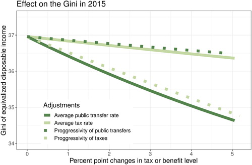
The results suggest that raising tax progressivity and the average rate of public transfers should reduce income inequality most. We run a simulation (for the full population) to observe this. We simulate the effect of increasing the average rate and changing the progressivity of taxes and public transfers on Lithuania using EU-SILC data. The effect of changing the progressivity or average rate of tax and public transfers on the Gini of Lithuania is illustrated in Figure 2. We simulate the average rate of taxes by increasing the taxes for all those who are currently paying taxes. We do a similar simulation for public transfers. We increase taxes and transfers by up to 5 percentage points of market income after public transfers. We increase the progressivity of taxes by increasing taxes by up to 5 percentage points for the top quintile of households that are sorted by market incomes and redistributing this gain to all other quintiles. The redistribution is also progressive. For example, if we were to increase taxes on the top quintile by 10%, then the 4th quintile will get to pay about 10% fewer taxes, the third will pay 20% less, the second 30% less and the first will pay 40% less. A scalar is added so that the reduction in taxes for the four bottom quintiles equals the increase in taxes for the top quantile. We increase the progressivity of public transfers by increasing transfers received by up to 5 percentage points for the bottom quintile of households that are sorted by market incomes and redistributing the cost to all other quintiles in a similar manner as for taxes. The simulations confirm that increasing the average rate of public transfers has a much higher effect on the Gini than raising taxes by the same amount. Increasing tax progressivity has a larger effect than increasing public transfer progressivity.

Figure 2. Simulating the effect of changes in progressivity and average rate of tax and public transfers on the Gini coefficient of equivalised disposable income in Lithuania.

6. Conclusions

We have tackled three questions and each of them is elaborated in this study. We have also suggested possible improvements for future studies.

First, we have run three statistical tests and found that equivalised income inequality in Lithuania is in all cases one of the highest in the EU. Specifically, we have tested for accuracy of estimates by estimating their standard errors, the inequality measure used as well as different equivalence scales. In all cases, equivalised income inequality in Lithuania is found to be one of the highest across the EU.

Second, we have investigated why equivalised income inequality in Lithuania is higher compared to the EU by using univariate decomposition techniques. We have found large inequalities between and within many groups of households in the country. In all cases, the within-group inequality contributes more to equivalised income inequality in Lithuania and the EU. It means that this inequality is higher within households of similar observable characteristics rather than between households of different characteristics. Inequalities within the unemployed and those working in the agricultural sector are especially prominent. Nevertheless, between-contributions are also significant for Lithuania, suggesting where policy can look into deeper. The largest between-group inequalities lie between the employed and the rest of the population. Moreover, this type of inequality has been rising over time. As the factor decomposition shows, the large between-group inequality contribution can be explained by unequal distribution of labour income, especially – self-employment income.

Third, we analysed the extent to which equivalised income inequalities stemming from the market income are offset by taxes and transfers. Specifically, we analysed the marginal and redistributive effects of Lithuania's taxes and transfers and compared this to the EU. The marginal decomposition of the Gini coefficient of equivalised disposable income by factors confirms that an increase in tax and transfer income reduces equivalised income inequality while an increase in labour income increases it. The way that the tax and transfer system is currently designed, the average marginal contribution is more than twice higher for transfers compared to taxes, and that among the transfers the role of the old-age pensions is the highest. Similarly, the analysis of the redistributive effect of the taxes and public transfer income also showed that these two income sources reduce income inequality. However, the redistributive impact of taxes in Lithuania is almost two times smaller than in the EU, while public transfers are about 50% smaller. The redistributive effect of taxes for the self-employed is negative in Lithuania and therefore reinforces income inequality, while taxes reduce inequality amongst the self-employed in the EU. This means that the current tax system and tax evasion/avoidance of higher-income households are likely to be responsible for a larger self-employment income contribution to inequality in Lithuania as opposed to EU.

We also decomposed the redistributive effect into the progressivity and the average rate of tax and public transfers effect. We find that the tax progressivity and the average rate of public transfers in particular are lower in Lithuania as compared to the EU. The results suggest that raising tax progressivity and the average rate of public transfers would reduce equivalised income inequality most.

The estimates of equivalised income inequality may have several drawbacks. First, there is a large shadow economy in Lithuania, with some estimates exceeding 25% of GDP in 2013 and 2015 (see Schneider, 2013; Žukauskas, 2016). Even though survey respondents are informed that their data will not be used for tax purposes, some of them may still be unwilling to disclose information on their true income received. It remains unclear how this affects equivalised income inequality because it depends on the income distribution within the shadow economy together with the income distribution of the observed economy. Additionally, this estimate may cause problems when comparing households across countries, since the size of the shadow economy is particularly large in Lithuania. Second, as has been already pointed out various times, EU-SILC undersamples the income of rich individuals in all countries (especially capital income (Navickė & Lazutka, 2018)) – something that the survey weights do not correct for. Including the rich will result in higher measures of equivalised income inequality in Lithuania. However, equivalised income inequality will rise in other EU countries as well. Therefore, the relative position of Lithuania vis-a-vis other countries may not change so much. Nevertheless, the alternative Household Finance and Consumption Survey (HFCN, 2019) could partly correct for both of these shortcomings, as it has data on consumption, which can be used to estimate the shadow economy and oversample the wealthy households for Lithuania along with many other EU countries. Furthermore, greater access to administrative data would be yet another path to take.

Future studies can also consider using an alternative methodology, for example, by using multivariate techniques to decompose equivalised income inequality. This was not the focus of the current study because the results of a multivariate decomposition depend on all variables by which the Gini is decomposed, and there is no consensus on which should be included. Furthermore, variables available to some countries are less available in others in the EU-SILC. Nevertheless, our additional check using a multivariate decomposition technique as in Social Situation Monitor (2017) does not contradict the results. Additionally, one may look into income inequality between individuals instead of households.

Disclosure statement

No potential conflict of interest was reported by the author(s).

Notes on contributors

Nerijus Černiauskas, Phd student of Economics at Vilnius University working on income inequality in Lithuania.

Dr. Andrius Čiginas, Researcher on statistics and probability at Vilnius University.

Appendices

$\mathcal{U}=\{1,\dots ,N\}$ is the set representing elements of the finite survey population, and $y_1,\dots ,y_N$ are values of the variable of interest (income) in $\mathcal{U}$. The subset $s=\{i_1,\dots ,i_n\}$ of $\mathcal{U}$ is the sample, while $w_i$ and $i\in s$ are the corresponding survey weights. We use the estimator(A1) $\hat{G}=\frac{2}{\hat{\mu }}\left(\frac{1}{\hat{N}}\sum _{i\in s}{w}_i{y}_i\hat{F}\left(y_i\right)-\frac{1}{{\hat{N}}^2}\sum _{i\in s}{w}_i{y}_i\sum _{i\in s}{w}_i\hat{F}\left(y_i\right)\right)$(A1) of the Gini coefficient (1(1) $G=\frac{2Cov(y,F(y\left)\right)}{\mu },$(1) ), constructed in line with Berger (2008), where $\hat{F}\left(y_i\right)$ are values of the estimated distribution function(A2) $\hat{F}\left(y\right)=\frac{1}{\hat{N}}\sum _{j\in s}{w}_j\mathbb{I}\{y_j\le y\}\mathrm{w}\mathrm{i}\mathrm{t}\mathrm{h}\hat{N}=\sum _{j\in s}{w}_j,$(A2) and$\hat{\mu }=\frac{1}{\hat{N}}\sum _{j\in s}{w}_j{y}_j.$Here $\mathbb{I}\{\cdot \}$ stands for the indicator function. Estimators of the subgroup and factor decompositions are constructed using similar plug-in principles.

Appendix 1. Subgroup decompositions

We give the decomposition of (A1(A1) $\hat{G}=\frac{2}{\hat{\mu }}\left(\frac{1}{\hat{N}}\sum _{i\in s}{w}_i{y}_i\hat{F}\left(y_i\right)-\frac{1}{{\hat{N}}^2}\sum _{i\in s}{w}_i{y}_i\sum _{i\in s}{w}_i\hat{F}\left(y_i\right)\right)$(A1) ) by groups as in Yitzhaki and Lerman (1991). Let $s=s_1\cup \cdots \cup s_L$ be a division of the sample by non-overlapping groups. Denote(A3) ${\hat{N}}_l=\sum _{j\in s_l}{w}_j,{\hat{P}}_l=\frac{{\hat{N}}_l}{\hat{N}},\hat{m}=\frac{1}{\hat{N}}\sum _{j\in s}{w}_j{y}_j,{\hat{m}}^{\left(l\right)}=\frac{1}{{\hat{N}}_l}\sum _{j\in s_l}{w}_j{y}_j,{\hat{F}}^{\left(l\right)}=\frac{1}{{\hat{N}}_l}\sum _{i\in s_l}{w}_i\hat{F}\left(y_i\right),$(A3) where ${\hat{N}}_l$ is the estimated population size in the subgroup l, the quantity ${\hat{P}}_l$ is the estimated population share, $\hat{m}$ is the estimated mean of the survey variable in $\mathcal{U}$, ${\hat{m}}^{\left(l\right)}$ is the estimated mean in the subgroup, and ${\hat{F}}^{\left(l\right)}$ is the estimate of the average of global ranks in the subgroup l. Consider the values ${\hat{F}}_l\left(y_i\right)$ and ${\hat{F}}_{L\mathrm{\setminus }l}\left(y_i\right)$, $i\in s$, of the estimated distribution functions${\hat{F}}_l\left(y\right)=\frac{1}{{\hat{N}}_l}\sum _{j\in s_l}{w}_j\mathbb{I}\{y_j\le y\}\mathrm{a}\mathrm{n}\mathrm{d}{\hat{F}}_{L\mathrm{\setminus }l}\left(y\right)=\frac{1}{\hat{N}-{\hat{N}}_l}\sum _{j\in s\mathrm{\setminus }{s}_l}{w}_j\mathbb{I}\{y_j\le y\}$in the subgroup l and outside this subgroup, respectively. Introduce the notations$\hat{c}ov(m^{\left(l\right)},F^{\left(l\right)})=\sum _{l=1}^L{\hat{P}}_l\left({\hat{m}}^{\left(l\right)}-\sum _{l=1}^L{\hat{P}}_l{\hat{m}}^{\left(l\right)}\right)\left({\hat{F}}^{\left(l\right)}-\sum _{l=1}^L{\hat{P}}_l{\hat{F}}^{\left(l\right)}\right)$and${\hat{c}ov}_l(y,F_l(y\left)\right)=\frac{1}{{\hat{N}}_l}\sum _{i\in s_l}{w}_i(y_i-{\hat{m}}^{\left(l\right)})\left({\hat{F}}_l\left(y_i\right)-\frac{1}{{\hat{N}}_l}\sum _{i\in s_l}{w}_i{\hat{F}}_l\left(y_i\right)\right),$and${\hat{c}ov}_l(y,F_l(y)-F_{L\mathrm{\setminus }l}(y\left)\right)={\hat{c}ov}_l(y,F_l(y\left)\right)-\frac{1}{{\hat{N}}_l}\sum _{i\in s_l}{w}_i(y_i-{\hat{m}}^{\left(l\right)})\left({\hat{F}}_{L\mathrm{\setminus }l}\left(y_i\right)-\frac{1}{{\hat{N}}_l}\sum _{i\in s_l}{w}_i{\hat{F}}_{L\mathrm{\setminus }l}\left(y_i\right)\right).$Then the estimated decomposition by groups is written as(A4) $\hat{G}=\underset{\mathrm{W}\mathrm{i}\mathrm{t}\mathrm{h}\mathrm{i}\mathrm{n}}{\underbrace{\sum _{l=1}^L{\hat{S}}_l{\hat{G}}_l}}+\underset{\mathrm{S}\mathrm{t}\mathrm{r}\mathrm{a}\mathrm{t}\mathrm{i}\mathrm{f}\mathrm{i}\mathrm{c}\mathrm{a}\mathrm{t}\mathrm{i}\mathrm{o}\mathrm{n}}{\underbrace{\sum _{l=1}^L{\hat{S}}_l{\hat{G}}_l{\hat{Q}}_l\left({\hat{P}}_l-1\right)}}+\underset{\mathrm{B}\mathrm{e}\mathrm{t}\mathrm{w}\mathrm{e}\mathrm{e}\mathrm{n}}{\underbrace{\frac{2\hat{c}ov(m^{\left(l\right)},F^{\left(l\right)})}{\hat{m}}}},$(A4) where${\hat{S}}_l={\hat{P}}_l\frac{{\hat{m}}^{\left(l\right)}}{\hat{m}},{\hat{G}}_l=\frac{2{\hat{c}ov}_l(y,F_l(y\left)\right)}{{\hat{m}}^{\left(l\right)}},{\hat{Q}}_l=\frac{{\hat{c}ov}_l(y,F_l(y)-F_{L\mathrm{\setminus }l}(y\left)\right)}{{\hat{c}ov}_l(y,F_l(y\left)\right)}.$Here the component ${\hat{S}}_l$ represents the share of the survey variable, ${\hat{G}}_l$ is the estimated within-group Gini coefficient, and the part ${\hat{Q}}_l$ is the estimated stratification term.

Appendix 2. Factor decompositions

We write down an estimate of the factor decomposition by Lerman and Yitzhaki (1985). Write $y_i=\sum _{k=1}^K{y}_i^{\left(k\right)}$, where k is a factor of the survey variable. Consider the values $\hat{F}\left(y_i\right)$ and $\hat{F}\left(y_i^{\left(k\right)}\right)$, $i\in s$, of distribution function (A2(A2) $\hat{F}\left(y\right)=\frac{1}{\hat{N}}\sum _{j\in s}{w}_j\mathbb{I}\{y_j\le y\}\mathrm{w}\mathrm{i}\mathrm{t}\mathrm{h}\hat{N}=\sum _{j\in s}{w}_j,$(A2) ) and denote the expressions$\hat{c}ov(y^{\left(k\right)},F(y\left)\right)=\frac{1}{\hat{N}}\sum _{i\in s}{w}_i{y}_i^{\left(k\right)}\hat{F}\left(y_i\right)-\frac{1}{{\hat{N}}^2}\sum _{i\in s}{w}_i{y}_i^{\left(k\right)}\sum _{i\in s}{w}_i\hat{F}\left(y_i\right)$and$\hat{c}ov(y^{\left(k\right)},F(y^{\left(k\right)}\left)\right)=\frac{1}{\hat{N}}\sum _{i\in s}{w}_i{y}_i^{\left(k\right)}\hat{F}\left(y_i^{\left(k\right)}\right)-\frac{1}{{\hat{N}}^2}\sum _{i\in s}{w}_i{y}_i^{\left(k\right)}\sum _{i\in s}{w}_i\hat{F}\left(y_i^{\left(k\right)}\right).$Also, introduce the weighted means${\hat{\mu }}^{\left(k\right)}=\frac{1}{\hat{N}}\sum _{j\in s}{w}_j{y}_j^{\left(k\right)}.$Then the estimated decomposition by factors is(A5) $\hat{G}=\sum _{k=1}^K{\hat{T}}_k=\sum _{k=1}^K{\hat{R}}_k{\hat{G}}_k{\hat{S}}_k,$(A5) where${\hat{R}}_k=\frac{\hat{c}ov(y^{\left(k\right)},F(y\left)\right)}{\hat{c}ov(y^{\left(k\right)},F(y^{\left(k\right)}\left)\right)},{\hat{G}}_k=\frac{2\hat{c}ov(y^{\left(k\right)},F(y^{\left(k\right)}\left)\right)}{{\hat{\mu }}^{\left(k\right)}},{\hat{S}}_k=\frac{{\hat{\mu }}^{\left(k\right)}}{\hat{\mu }}.$Here ${\hat{R}}_k$ is the estimate of the so-called Gini correlation between the survey variable and its kth component, ${\hat{G}}_k$ represents the Gini index of factor k, and ${\hat{S}}_k$ is the share of factor. For a small change in the kth factor, the expression of marginal effects is(A6) $\frac{\mathrm{\partial }\hat{G}}{\mathrm{\partial }{e}_k}={\hat{S}}_k({\hat{R}}_k{\hat{G}}_k-{\hat{G}}_k),$(A6) see Lerman and Yitzhaki (1985).

References

- Aghion, P., Caroli, E., & Garcia-Penalosa, C. (1999). Inequality and economic growth: The perspective of the new growth theories. Journal of Economic Literature, 37(4), 1615–1660. https://doi.org/10.1257/jel.37.4.1615
- Atkinson, A. B. (1970). On the measurement of inequality. Journal of Economic Theory, 2(3), 244–263. https://doi.org/10.1016/0022-0531(70)90039-6
- Atkinson, A. B., & Piketty, T. (2010). Top incomes: A global perspective. Oxford University Press.
- Berger, Y. G. (2008). A note on the asymptotic equivalence of Jackknife and linearization variance estimation for the Gini coefficient. Journal of official statistics. 24(4). https://www.researchgate.net/publication/277826713_A_Note_on_the_Asymptotic_Equivalence_of_Jackknife_and_Linearization_Variance_Estimation_for_the_Gini_Coefficient
- Buhmann, B., Rainwater, L., Schmaus, G., & Smeeding, T. M. (1988). Equivalence scales, well-being, inequality, and poverty: Sensitivity estimates across ten countries using the Luxembourg income study (LIS) database. Review of Income and Wealth, 34(2), 115–142. https://doi.org/10.1111/roiw.1988.34.issue-2 doi: 10.1111/j.1475-4991.1988.tb00564.x
- Causa, O., & Hermansen, M. (2017). Income redistribution through taxes and transfers across OECD countries (No. 1453). https://doi.org/10.1787/bc7569c6-en. https://www.oecd-ilibrary.org/content/paper/bc7569c6-en
- Černiauskas, N., & Jousten, A. (2020, February). Statutory, effective and optimal net tax schedules in Lithuania (Bank of Lithuania Working Paper Series 72). Bank of Lithuania. https://ideas.repec.org/p/lie/wpaper/72.html
- Černiauskas, N., Sologon, D. M., O'Donoghue, C., & Tarasonis, L. (2020, January). Changes in income inequality in Lithuania: The role of policy, labour market structure, returns and demographics (Bank of Lithuania Working Paper Series 71). Bank of Lithuania. https://ideas.repec.org/p/lie/wpaper/71.html
- Chiappori, P.-A., & Meghir, C. (2015). Intrahousehold Inequality. In A.B Atkinson & F Bourguignon (Eds.), Handbook of Income Distribution (Vol. 2, pp. 1369–1418). Elsevier.
- Cingano, F. (2014). Trends in income inequality and its impact on economic growth (No. 163). https://EconPapers.repec.org/RePEc:oec:elsaab:163-en
- Cowell, F. A. (2000). Measurement of inequality. Handbook of Income Distribution, 1, 87–166. https://doi.org/10.1016/S1574-0056(00)80005-6
- Cowell, F. (2011). Measuring inequality. Oxford University Press.
- Das, T., & Parikh, A. (1982). Decomposition of inequality measures and a comparative analysis. Empirical Economics, 7(1), 23–48. https://doi.org/10.1007/BF02506823
- Elbers, C., Lanjouw, P., Mistiaen, J. A., & Özler, B. (2008). Reinterpreting between-group inequality. The Journal of Economic Inequality, 6(3), 231–245. https://doi.org/10.1007/s10888-007-9064-x
- Eurostat. (2018a). EU statistics on income and living conditions (EU-SILC) methodology -- Distribution of income. https://ec.europa.eu/eurostat/statistics-explained/index.php?title=EU_statistics_on_income_and_living_conditions_(EU-SILC)_methodology_-_distribution_of_income
- Eurostat. (2018b). EU statistics on income and living conditions (EU-SILC) methodology – Concepts and contents. https://ec.europa.eu/eurostat/statistics-explained/index.php?title=EU_statistics_on_income_and_living_conditions_(EU-SILC)_methodology_%E2%80%93_concepts_and_contents#Adjusted_cross_sectional_weight_.28RB050a.29
- Eurostat. (2018c). European union statistics on income and living conditions (EU-SILC). https://ec.europa.eu/eurostat/web/microdata/european-union-statistics-on-income-and-living-conditions
- Eurostat. (2020). Gini coefficient of equivalised disposable income – EU-SILC survey. https://ec.europa.eu/eurostat/data/database
- Garner, T. I., & Terrell, K. (1998). A gini decomposition analysis of inequality in the Czech and Slovak Republics during the transition. The Economics of Transition, 6(1), 23–46. https://doi.org/10.1111/ecot.1998.6.issue-1 doi: 10.1111/j.1468-0351.1998.tb00035.x
- Goedemé, T. (2013). How much confidence can we have in EU-SILC? Complex sample designs and the standard error of the Europe 2020 poverty indicators. Social Indicators Research, 110(1), 89–110. https://doi.org/10.1007/s11205-011-9918-2
- Grigoli, F., & Robles, A. (2017). Inequality overhang. International Monetary Fund.
- HFCN. (2019). Household finance and consumption network (HFCN). ECB. https://www.ecb.europa.eu/pub/economic-research/research-networks/html/researcher_hfcn.en.html
- IMF. (2016). Republic of Lithuania, selected issues (IMF Country Report No. 16/126).
- Jenkins, S. (2017). The measurement of income inequality (pp. 17–52). Routledge.
- Joumard, I., Pisu, M., & Bloch, D. (2013). Tackling income inequality: the role of taxes and transfers. OECD Journal: Economic Studies, 2012(1), 37–70. https://doi.org/10.1787/eco_studies-2012-5k95xd6l65lt
- Kakwani, N. C. (1977). Measurement of tax progressivity: An international comparison. The Economic Journal, 87(345), 71–80. https://doi.org/10.2307/2231833
- Lazutka, R. (2017). Pervedimų, Valstybės Teikiamų Prekiuų ir Paslaugų Vaidmuo. In Pajamų Nelygybė Lietuvoje, October 5th, Lietuvos Nacionalinė Martyno Mažvydo Biblioteka. Bank of Lithuania. https://www.lb.lt/uploads/documents/files/Lazutka.pdf
- Lerman, R. I., & Yitzhaki, S. (1985). Income inequality effects by income source: A new approach and applications to the United States. The Review of Economics and Statistics, 67(1), 151–156. https://doi.org/10.2307/1928447
- Lis, M. (2018, September). Lithuania's pension system in the international persective (Technical report).
- Navickė, J., & Lazutka, R. (2018). Distributional implications of the economic development in the baltics: Reconciling micro and macro perspectives. Social Indicators Research, 138(1), 187–206. https://doi.org/10.1007/s11205-017-1645-x
- OECD. (2011). Divided we stand. https://doi.org/10.1787/9789264119536-en. https://www.oecd-ilibrary.org/content/publication/9789264119536-en
- OECD. (2015a). All on board. https://doi.org/10.1787/9789264218512-en. https://www.oecd-ilibrary.org/content/publication/9789264218512-en
- OECD. (2015b). In it together: Why less inequality benefits all. https://doi.org/10.1787/9789264235120-en. https://www.oecd-ilibrary.org/content/publication/9789264235120-en
- Ostry, J. D., & Berg, A. (2011). Inequality and unsustainable growth: Two sides of the same coin? https://www.imf.org/en/Publications/Staff-Discussion-Notes/Issues/2016/12/31/Inequalityand-Unsustainable-Growth-Two-Sides-of-the-Same-Coin-24686
- Ostry, J. D., Berg, A., & Tsangarides, C. G. (2014). Redistribution, inequality, and growth. International Monetary Fund.
- Pahl, J. (1995). His money, her money: Recent research on financial organisation in marriage. Journal of Economic Psychology, 16(3), 361–376. https://doi.org/10.1016/0167-4870(95)00015-G
- Plat, D. (2012). IC2: Inequality and concentration indices and curves (R package version 1.0-1). https://cran.r-project.org/web/packages/IC2/index.html
- Rao, J. N. K., Wu, C. F. J., & Yue, K. (1992). Some recent work on resampling methods for complex surveys. Survey Methodology, 18(2), 209–217. https://doi.org/10.1007/978-3-0348-8930-8_11
- Schneider, F. (2013). Size and development of the shadow economy of 31 european and 5 other OECD countries from 2003 to 2013: A further decline. http://politeia.org.ro/wp-content/uploads/2013/05/ShadEcEurope31_Jan2013.pdf
- Shorrocks, A. F. (1982). Inequality decomposition by factor components. Econometrica: Journal of the Econometric Society, 50(1), 193–211. https://doi.org/10.2307/1912537
- Social Situation Monitor. (2017). Research findings – Social situation monitor – Measurement and methodology. https://ec.europa.eu/social/home.jsp?langId=en
- SODRA. (2020). Contribution rates for employees. SODRA. https://www.sodra.lt/en/benefits/contributionrates/contribution-rates-for-employees
- Vogler, C., & Pahl, J. (1994). Money, power and inequality within marriage. The Sociological Review, 42(2), 263–288. https://doi.org/10.1111/j.1467-954X.1994.tb00090.x
- Yitzhaki, S. (1983). On an extension of the Gini inequality index. International Economic Review, 24(3), 617–628. https://doi.org/10.2307/2648789
- Yitzhaki, S., & Lerman, R. I. (1991). Income stratification and income inequality. Review of Income and Wealth, 37(3), 313–329. https://doi.org/10.1111/roiw.1991.37.issue-3 doi: 10.1111/j.1475-4991.1991.tb00374.x
- Zardo, T. L., & Goedemé, T. (2016). Notes on updating the EU-SILC UDB sample design variables, 2012–2014.
- Žukauskas, V. (2016). Lietuvos Šešėlinė Ekonomika, Lietuvos laisvosios rinkos institutas, Vilnius.
Appendices
is the set representing elements of the finite survey population, and
are values of the variable of interest (income) in
. The subset
of
is the sample, while
and
are the corresponding survey weights. We use the estimator
(A1)
(A1) of the Gini coefficient (Equation1
(1)
(1) ), constructed in line with Berger (Citation2008), where
are values of the estimated distribution function
(A2)
(A2) and
Here
stands for the indicator function. Estimators of the subgroup and factor decompositions are constructed using similar plug-in principles.