Conventional and unconventional monetary policies: effects on the Finnish housing market

ABSTRACT

This paper investigates how different types of monetary policy have affected house prices in Finland, a small euro area economy that has experienced pronounced business cycles over time. The analyses are carried out using the Bayesian structural vector autoregressive approach. Monetary policy interest rate shocks and balance sheet shocks are identified using zero and sign restrictions. The results reveal that both a policy interest rate shock and a balance sheet shock have a positive and temporary impact on house prices in Finland, with the response to a balance sheet shock being smaller and fading out faster. The peak of the effect of a policy rate shock on house prices in Finland arrives faster than in the whole euro area but the magnitudes of the peak impact are similar. The effect of a balance sheet shock on house prices is not notably different in Finland to what it is in the whole euro area.

KEYWORDS:

• Monetary policy
• house prices
• BSVAR
• zero and sign restrictions
• euro area

JEL CLASSIFICATION CODES:

• C32
• E30
• E42
• E52
• R31

1. Introduction

House prices played an important role in the global financial crisis of 2008–2010. The collapse of house prices led to a deleveraging process so that outstanding household debt suddenly exceeded property prices (Huber & Punzi, 2020). The economic boom of the 2000s was accompanied by an upsurge of house prices, and it also brought with it an increase in housing equity withdrawal and consumption. Even if house prices did not cause the crisis, they were important amplifiers of its consequences. Developments in house prices may strengthen and possibly even create macroeconomic cycles as housing wealth affects household consumption, construction activity and the financial sector (Oikarinen, 2007). As developments in the housing market are also likely to be of key importance for economic developments in the future, it is important to learn from the past about the impact they have.

In response to the global financial crisis, major central banks, including the European Central Bank (ECB), lowered their policy rates in order to ease liquidity conditions and stimulate economic growth. As the policy rates approached or reached the zero lower bound, other expansionary monetary policy measures were implemented in addition to the traditional steering of policy interest rates. These alternative measures are referred to as unconventional monetary policy, and include measures like large-scale asset purchases and forward guidance. As the use of conventional monetary policy measures was limited, unconventional monetary policy became the centre of the debate about the monetary toolkit. The aim of large-scale asset purchases was to lower long-term bond yields and long-term interest rates, including the interest rates on housing loans. This could cause changes in housing wealth. As housing wealth makes up a large share of total household wealth, it is important to study how unconventional monetary policy impacts house prices.

There is a rapidly growing literature on how unconventional monetary policy affects macroeconomic variables, but there are only a handful of studies about the effects on house prices, among them being Rahal (2016), Huber and Punzi (2020), Gabriel and Lutz (2017), Smith (2014), Renzhi (2018), and Rosenberg (2019). Only a couple of papers have explored the effect of unconventional monetary policy on house prices in the euro area, such as Rahal (2016) and Huber and Punzi (2020), and to the best of my knowledge there has not yet been any study of the impact of unconventional monetary policy on house prices in an individual euro area country. As there may be heterogeneity in the effects across the countries of the euro area and pooling the data may lead to biased inference (Nocera & Roma, 2017; Pesaran & Smith, 1995), it would be relevant to learn about the effects in an individual euro area country.

The analysis in the current paper focuses on Finland. It is intriguing to study an advanced welfare monetary union member country that over time has witnessed notably large rises and falls in house prices, and different monetary policy regimes. Finland is a small country but its GDP per capita is similar to that of the United Kingdom, Japan and Canada. What makes Finland also interesting is that it is in a monetary union, making it possible to investigate whether the response to different kinds of monetary policy shock is different in a small member country to what it is in the monetary union as a whole.

This paper studies the effects of conventional and unconventional monetary policy on house prices in Finland, a small open economy in the euro area. The emphasis is on Finland, but as the shocks are identified using also the variables of the whole euro area, the paper also discusses the effects on euro area variables. I first study how policy rate and balance sheet shocks affect house prices in Finland and the whole euro area, estimating the impulse response functions. Then I investigate how the impacts of the two kinds of monetary policy shock differ within Finland and within the euro area. Third, I evaluate whether there are differences between the responses in Finland and those in the whole euro area.

The impact of unconventional monetary policy on house prices in Finland has not yet been studied. There are some papers that study the influence of conventional monetary policy on house prices in Finland, such as Giuliodori (2005), who explores the impact of interest rate shocks on house prices in nine European countries, including Finland, using data for the period 1979Q3-1998Q4 in VAR models identified by Choleski decomposition. He finds that a contractionary monetary policy shock of 100 basis points is followed by a negative response of house prices, with the impact peaking at 1.8%. The results are, however, not statistically significant. Oikarinen (2009) uses quarterly data from 1975 to 1987 in a VECM model and finds that a positive interest rate shock of 100 basis points has a small, positive temporary impact of a bit less than 1% on real house prices. Using a sample from a later period even gives a negative effect.

The effect of unconventional monetary policy on macroeconomic variables in the euro area and in individual euro area countries including Finland has been studied in Elbourne et al. (2018). They use SVAR and VARX models and the unconventional monetary policy shock is identified using zero and sign restrictions. House prices are not included in the model. The empirical study of Elbourne et al. (2018) is carried out using monthly data for the period 2009M1-2016M11. The results indicate that an unconventional monetary policy shock has a very small and not statistically significant effect on output and prices, both in the euro area and in Finland individually.

I use the Bayesian structural vector autoregressive approach with an identification that uses a combination of zero and sign restrictions. This kind of identification of shocks is increasingly used in the literature, and Baumeister and Benati (2013), Peersman (2011), Schenkelberg and Watzka (2013), Boeckx et al. (2017), Rahal (2016), Weale and Wieladek (2016), and Nocera and Roma (2017) are all examples.

To quantify the effects of unconventional monetary policy I follow the strand of literature that uses innovations in the central bank’s balance sheet as a measure of unconventional monetary policy. Examples of this approach can be found in Peersman (2011), Gambacorta et al. (2014), Rahal (2016), Boeckx et al. (2017), Gupta and Jooste (2018), and Renzhi (2018). Another approach to identification found in the literature is the shadow interest rate, which is used for example by Huber and Punzi (2020) to investigate the effects of unconventional monetary policies on house prices in the United States, the United Kingdom, Japan and the euro area. However, using the shadow interest rate does not allow the effects of conventional and unconventional monetary policy to be distinguished separately. As an important objective of the current paper is to compare the effects of the two types of monetary policy shock on house prices, shadow interest rate cannot be employed and so balance sheet innovations are used. To identify a conventional monetary policy shock I use innovations in the overnight interest rate EONIA. Using a money market interest rate as a proxy for a monetary policy shock is quite common in the literature.

The results indicate that an exogenous decrease in the monetary policy interest rate has a small positive and temporary impact on house prices, both in Finland and in the whole euro area. The balance sheet shock has an even smaller effect on house prices in Finland and the euro area, and in both cases the effect of a balance sheet shock fades out faster than the effect of a policy rate shock.

The paper contributes to the literature in a number of ways. First, it contributes to the relatively scarce literature studying the effect of unconventional monetary policy on house prices. Second, this paper contrasts with the previous literature by being the first to explore the effect of unconventional monetary policy on house prices in an individual euro area country. Third, the paper is the first to compare the effects of conventional and unconventional monetary policy on house prices in a single euro area country.

The rest of the paper proceeds as follows. The next section introduces the benchmark VAR model and describes the data. Section 3 presents and discusses the identification scheme of the monetary policy shocks. Section 4 contains the results of the estimation, showing and commenting on the impulse response functions of the identified shocks. Section 5 describes the robustness checks. Section 6 concludes.

2. Model specification and data

To explore the responses of house prices to monetary policy shocks I set up a structural vector autoregressive (SVAR) model. Like most studies that use sign restrictions in the identification scheme, I employ the Bayesian approach for estimation and inference, since in case of inequality restrictions the models are set identified, not point identified. Frequentist confidence intervals in models identified with sign restrictions tend to be wide and not informative about the shape of the impulse response function, making it difficult to interpret the results economically (Kilian & Lütkepohl, 2017). For this reason, most of the studies that use sign restrictions follow the Bayesian approach.

First, I estimate the following reduced-form VAR model:(1) $Y_t=c+\sum _{i=1}^n{b}_i{Y}_{t-i}+u_t$(1) where $Y_t$ is a vector of endogenous variables, $c$ is a vector of constants, $b_i$s are matrices of the autoregressive coefficients of the lagged values of $Y_t$, $i$ is the number of lags in the model, and $u_t$ is a vector of residuals. To obtain orthogonal disturbances and to give economic meaning to the shocks, I transform the reduced-form VAR model into a structural form:(2) $A_0{Y}_t=B_0+\sum _{i=1}^n{B}_i{Y}_{t-i}+{\epsilon }_t$(2) where $A_0$ is the contemporaneous impact matrix of structural disturbances, $B_i$s are matrices of the structural coefficients of the lagged values of $Y_t$ and the reduced-form error terms $u_t$ are related to the mutually orthogonal structural errors (shocks) ${\epsilon }_t$in the following way:(3) $u_t=A_0^{-1}{\epsilon }_t$(3) The vector of endogenous variables is:(4) $Y_t=\left[GD{P}_t^{\ast },HIC{P}_t^{\ast },H{P}_t^{\ast },B{P}_t^{\ast },M_t^{\ast },R^{\ast },T^{\ast },GD{P}_t,HIC{P}_t,H{P}_t,B{P}_t,M_t\right]{}^{\mathrm{\prime }}$(4)

The model contains seven euro area variables, each marked with *, and five Finnish variables. Gross domestic product per capita¹ $(GD{P}_t^{\ast },GD{P}_t)$, harmonized indexes of consumer prices $(HIC{P}_t^{\ast },HIC{P}_t),$ house prices ($H{P}_t^{\ast },H{P}_t$), building permits per capita $(B{P}_t^{\ast },B{P}_t)$and mortgage interest rates $(M_t^{\ast },M_t)$are included for both the euro area and Finland, and the monetary policy rate $\left(R^{\ast }\right)$ and the central bank’s total assets per capita ($T^{\ast }$) only for the euro area, as the monetary policy shocks of individual euro area countries have to be identified through euro area variables. All the variables except the interest rates are in natural logarithms and have been multiplied by 100 for a better presentation of results. GDP, house prices and the central bank’s total assets were deflated by the HICP to obtain real variables. For robustness I also estimated the model using the GDP deflator instead of the HICP, and the results were very similar.

An interbank rate is used instead of the policy rate itself in the model, as the policy rate moves in discrete steps but the interbank rate reflects all the information currently available about the future direction of the policy rate (Elbourne et al., 2018). Money market rates are used a lot in the literature as the monetary policy interest rate variable. I have used the nominal euro overnight index average (EONIA), following Elbourne et al. (2018) among others. For robustness I also did the analysis using EURIBOR and MLF instead of EONIA and the results appeared to be quite similar (see Appendix B).

The dataset is of quarterly frequency. The period runs from 2009Q1 to 2018Q2. An overview of the data used in the paper is given in Appendix A. All the data time series except population were seasonally adjusted by using the X12-ARIMA method in Eviews. The population data are only available annually, and quarterly values were obtained by interpolation using the cubic spline approach. In the process of seasonal adjustments, the multiplicative approach was used, except for time series that contained negative numbers, in which case the additive approach was used.

The data are in levels, allowing for implicit cointegrating relationships (Sims et al., 1990), as widely used in the literature of VAR models such as Gambacorta et al. (2014), Rahal (2016), Boeckx et al. (2017), Cesa-Bianchi et al. (2015), and Cesa-Bianchi et al. (2018). The basic assumption of this approach is that a VAR using data in levels implicitly takes cointegrated relationships into account. As I am using the Bayesian approach for estimation and inference, the use of data in levels is also supported by the argument in Sims et al. (1990) that the Bayesian inference does not need to take non-stationarity into account as the likelihood function retains its Gaussian shape also in case of non-stationarity.

Two lags are used, following a large amount of literature employing quarterly data such as Baumeister and Benati (2013), Calza et al. (2013), Aspachs-Bracons and Rabanal (2011), and others. The Schwarz information criterion and the Hannah-Quinn information criterion suggested that one lag should be used. However, I still include two lags as is typical in the literature, because adding an additional unnecessary lag results only in a loss of estimation efficiency, but excluding a necessary lag is a misspecification (Elbourne et al., 2018).

The estimations are carried out in the BEAR Toolbox of MATLAB (Dieppe et al., 2016). I use the independent Normal-Wishart prior, as the Normal-Wishart prior cannot be used in case of block exogeneity. Unlike, say, the Minnesota prior, the Normal-Wishart priors do not assume that the variance-covariance matrix of the reduced-form residuals is known. The toolbox uses the model estimation algorithm of Arias et al. (2018) in case of structural identification with sign restrictions. The algorithm draws a posterior distribution over the orthogonal reduced-form parametrization and transforms the draws into structural parametrization (Arias et al., 2018). The draws that satisfy the restrictions are kept, while the other draws are rejected. Successful draws are used to generate the impulse response functions, displaying the credible sets derived from the posterior distributions.

The BEAR Toolbox’s default values for the hyperparameters, that are the standard values of the literature for computing the mean and variance of the prior distribution for the VAR coefficients, are used. The autoregressive coefficient is 0.8, overall tightness is 0.1, cross-variable weighting is 0.5, lag decay is 2, exogenous variable tightness has the value 100, and block exogeneity shrinkage is 0.001. A total of 1000 successful draws from the posterior are used to generate the impulse response functions, following for example Peersman (2011) and Rahal (2016).

3. Identification scheme

In this paper I employ a partially identified model. To investigate the effects of different types of monetary policy shock on house prices, two shocks are identified. To sharpen the identification, the identification scheme combines zero and sign restrictions, using the algorithm of Arias et al. (2018). A combination of zero and sign restrictions in the identification scheme is increasingly used in the literature, for example in Baumeister and Benati (2013), Peersman (2011), Schenkelberg and Watzka (2013), Gambacorta et al. (2014), Boeckx et al. (2017), Weale and Wieladek (2016), Rahal (2016), and Nocera and Roma (2017).

The identification scheme of monetary policy shocks (see Table 1) is built on Rosenberg (2019). As Finland is in a monetary union, monetary policy shocks first have to be identified through their impact on the euro area variables and only then can the influence on Finnish domestic variables be studied. The assumption of block exogeneity, which is that the variables of a small member country do not contemporaneously affect the euro area variables, is added to the identification scheme of Rosenberg (2019), following Kilian and Lütkepohl (2017) and Mumtaz and Surico (2009). Also, compared to Rosenberg (2019) I have added the HICPs of the euro area and Finland as additional variables. HICP is used in models investigating the effect of monetary policy shocks on house prices in, for example, Nocera and Roma (2017) and Huber and Punzi (2020).

Table 1. Identification of monetary policy shocks.

	GDP*	HICP*	HP*	BP*	M*	R*	T*	GDP	HICP	HP	BP	M
Policy rate shock	0	0	>0	0	<0	<0	0	0	0	>0	0	<0
Balance sheet shock	0	0	>0	0	<0	0	>0	0	0	>0	0	<0

Note: * marks the euro area variables, the other variables are the domestic variables of Finland.

Two shocks are identified, a policy rate shock and a balance sheet shock. The zeros in Table 1 indicate no contemporaneous response of the shock on the variable. Inequalities show the sign of the effect on that variable on impact and in the two following quarters (following e.g. Rahal, 2016).

I assume that the house prices in the euro area and in Finland would contemporaneously increase in response to both types of monetary policy shocks. In other words, I allow for the possibility that the house prices could respond to the change in the cost of borrowing already in the quarter of the shock. By placing a sign restriction on the response of house prices in the euro area and in Finland to a monetary policy shock the current paper follows the empirical literature that argues that house prices react almost instantaneously to a monetary policy innovation (e.g. Bjørnland & Jacobsen, 2010; Huber & Punzi, 2020; Nocera & Roma, 2017; and Ume, 2018). This assumption is grounded by macroeconomic theory as house prices being asset prices are forward-looking and will respond fast to monetary policy shocks (Bjørnland & Jacobsen, 2010). The immediate effect of changes in monetary policy on asset prices is assumed in a large amount of literature, including for example Rigobon and Sack (2004), Bernanke and Kuttner (2005), Bohl et al. (2008) and Alessi and Kerssenfischer (2019).

The contemporaneous impacts of both types of monetary policy shock on GDP, consumer prices and the housing supply are restricted to zero. Most of the literature on monetary policy shocks assumes that these shocks have only a lagged impact on GDP and consumer prices, as in Peersman (2011), Gambacorta et al. (2014), Boeckx et al. (2017), and Nocera and Roma (2017). It can be assumed that the housing supply is quite inelastic in the short run, as new construction takes time to plan and build. The housing supply variable in this paper is the number of square metres of building permits and although building time is not reflected in that variable, it can be assumed that building permits are not obtained instantly and hence the one-period lag can be considered justified.

Following, for example, Peersman (2011), Rahal (2016), Weale and Wieladek (2016) and Nocera and Roma (2017), the mortgage interest rate is restricted to decrease on impact in case of both identified shocks. A cut in the policy rate would induce a fall in the money market interest rates that in turn would be passed through to lower bank lending rates, including mortgage rates. A rise in liquidity due to balance sheet policies would increase the credit supplied by the banks, and that in turn would reduce lending rates (Peersman, 2011).

As a policy rate shock is identified as an exogenous innovation in the monetary policy rate (proxied by EONIA in this paper), I restrict that variable to decrease in case of an expansionary policy rate shock. Since I define a balance sheet shock as a monetary policy shock that leaves the policy rate unchanged, I restrict the policy rate variable to have only a lagged impact in case of a balance sheet shock. As the central bank’s total assets are the variable for the balance sheet innovations in my paper, I restrict the central bank’s total assets to increase contemporaneously after an expansionary balance sheet shock, following, for example, Schenkelberg and Watzka (2013), Gambacorta et al. (2014), and Rahal (2016). I also assume that the policy rate shock can impact the central bank’s total assets only with a lag.

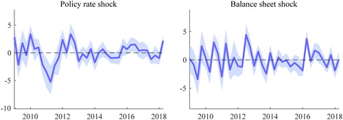
The times series for the shocks identified are shown in Appendix C. The econometrically identified shocks are reasonable and broadly are in line with information on the monetary policy decisions of the ECB. The identified monetary policy rate shocks capture, for example, the decrease of the key interest rates in 2009 and also the decrease of the policy interest rates in the second half of 2011 after a period of them being unchanged or even slightly increasing for some quarters. Since the year 2013 there are no notably large shocks. However, in 2014 a small negative shock is observed, that could be tied to the introduction of a negative policy interest rate.

The identified balance sheet shocks seem to reflect, for example, the ECB decision to continue its main refinancing operation with full allotment in 2010 and the announcement of outright monetary transactions programme in 2012. Also, for example, the monetary policy decision of the expansion of the monthly purchases under the asset purchase programme, and the announcement of a new series of targeted longer-term refinancing operations in 2016 can be seen to be captured by the shocks.

4. Results

This section presents the responses to the policy rate and balance sheet shocks of house prices and other variables in the model. The 68% credible sets (the 16th and 84th percentiles) of the impulse response functions (IRFs) are reported, following the standard in the sign restrictions literature. The credible set reflects model uncertainty as well as sampling uncertainty (Gambacorta et al., 2014). Model uncertainty comes from the model being set identified, not point identified. Hence the data are potentially consistent with a number of structural models that are all admissible (Kilian & Lütkepohl, 2017). The median is also displayed in the figures, following for example Uhlig (2005).

The medians are commented in the interpretation of the impulse response functions, as in Uhlig (2005). I use the term ‘significant’ to refer to the credible set excluding zero as in Dieppe et al. (2016) and Nocera and Roma (2017), and so the term ‘not significant’ is used in this paper for a credible set containing zero.

The shock size in Figure 1 is one standard deviation as common in the literature using structural VAR models (e.g. Boeckx et al., 2017; Cesa-Bianchi, 2013; Christiano & Eichenbaum, 2005; Gambacorta et al., 2014; Peersman, 2011; Uhlig, 2005). I have followed the paper of Peersman (2011) in using shocks of the size of one standard deviation in case of comparing the effects of two types of monetary policy shocks. Also, Gambacorta et al. (2014) have compared the effects of different types on monetary policy shock, based on the impulse responses of shocks of the size of one standard deviation. This makes it possible to compare the impacts of shocks to different variables as one standard deviation shock represents a typical shock to the respective variable.

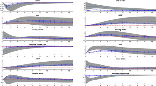
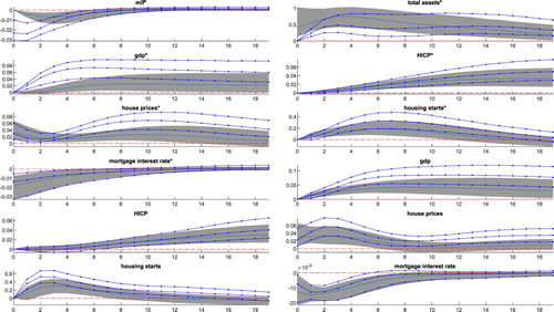
Figure 1. Impulse responses to policy rate and balance sheet shocks in Finland and the euro area (2009Q1-2018Q2). Notes: The area bordered by lines displays the impact of policy rate shocks, the shadowed area shows the impact of the balance sheet shocks (68% credible set). The line within a credible set represents the median of the impulse responses. * is used to mark the euro area variables, the other variables are the domestic variables of Finland.

Exogenous innovations to the interest rate bring a decrease in EONIA of around 3.5 basis points, and exogenous innovations to the total assets of the ECB correspond to an increase of about 0.4%.

The results displayed in Figure 1 with the area bordered with lines indicate that a cut of 3.5 basis points in the euro area policy interest rate is followed in Finland by a rise in house prices that peaks at 0.07% two quarters after the shock. The price level is still 0.02% higher five years after the shock. The small impact of a policy rate shock on house prices in Finland is consistent with earlier studies such as Giuliodori (2005) and Oikarinen (2009). The policy rate shock has a positive impact on house prices also in the whole euro area like it does in Finland. The impact peaks around the 8th quarter at about 0.05%. The peak impact is reached later than in Finland. The effect dies out in about 4.5 years, and hence is also quite persistent as in case of Finland. The persistent effect of a policy rate shock on house prices in the euro area has also been found by, for example, Nocera and Roma (2017).

An expansionary balance sheet shock amounting to an increase of about 0.4% in the total assets of the ECB, also presented in Figure 1 (depicted with shadowed area) has a small, positive and temporary effect on house prices in Finland. The median response peaks at the magnitude of 0.035% and is reached in the period of the impact of the shock. The effect dies out in a year. The impact of a balance sheet shock in the euro area is of the same magnitude as in Finland. It peaks at around 0.035% also in the impact period of the shock as in case of Finland. The effect is more persistent than in Finland, fading out in the 9th quarter. As indicated in the introduction to this paper the literature on the effect of unconventional monetary policies on house prices is as yet very limited, but comparing the results of the current paper with those of the few papers that have studied the impact of unconventional monetary policy on house prices in the euro area shows that the results of this paper are in line with the earlier literature. There is a very small impact in case of most models in Rahal (2016) as well as in Huber and Punzi (2020). Huber and Punzi (2020) suggest that a possible explanation of the weaker response of housing variables in the euro area than in the US and the UK is that the individual members of the euro area tend to be less integrated.

A policy rate shock appears to have a larger and more persistent impact on house prices than a balance sheet shock does in Finland and in the euro area as a whole. In Finland though, the peak of the effect of a policy rate shock on house prices arrives faster than it does in the whole euro area. The impact peaks at roughly the same magnitude in Finland and the euro area. The effect of a balance sheet shock on house prices dies out much faster in Finland and in the total euro area compared to the effect of the policy rate. The peak magnitudes of the effects are smaller in case of a balance sheet shock than in case of a policy rate shock. These results would indicate that a standard deviation sized policy rate innovation would influence the house prices more strongly than a standard deviation sized balance sheet shock.

Turning briefly to the impact that the two types of monetary policy shock have on other variables of the model, it can be seen from Figure 1 that the impact on GDP is quite similar to the impact on house prices in magnitude of the peak effect in case of the effect of a policy rate shock in both areas and in case of the effect of a balance sheet shock in Finland. The impact of a policy rate shock on Finnish GDP peaks at around 0.07%; the effect is smaller for euro area GDP, being around 0.05%. A similarly small impact of a policy rate shock on GDP in Finland and in the euro area has also been found in earlier literature such as Giuliodori (2005) for Finland and Peersman (2011), or Errit and Uusküla (2014) for the euro area. The impact of a balance sheet shock on the GDP of Finland is very similar to the impact on house prices: it is positive and temporary, and peaks at the magnitude of about 0.03%. In the euro area a balance sheet shock does not appear to have a significant effect on GDP.

The small response of house prices and output to a balance sheet shock can be considered to be consistent with earlier studies. The effect of an unconventional monetary policy shock on house prices has only been studied in a few papers and a very small response in the euro area can be seen in those studies as well. The response of output can be compared to that in Elbourne et al. (2018), where the effect is also very small and not significant in both the euro area and Finland as an individual country. Elbourne et al. (2018) also study the impact on consumer prices in the euro area and individual euro area countries and the effect on that variable also appears to be notably small and not significant, again both at the level of the whole monetary union and in Finland. The latter conclusion is also consistent with the findings of the current paper as the response of the HICP of the euro area and the HICP of Finland to a balance sheet shock is very small and initially not significant for several quarters.

The impact of a policy rate shock on housing starts is faster and peaks at a higher magnitude in Finland than in the whole euro area. The effect dies out in the 11th quarter in case of Finland and in the 12th quarter in case of the euro area. In Finland there is no effect of a balance sheet shock on housing starts. In the euro area the effect is not significant until around the second quarter and after that there is a small positive effect on housing starts until the end of the second year. The effect of a policy rate shock on housing starts is much larger than the effect of a balance sheet shock on housing starts in case of Finland and the euro area.

The response of ECB total assets to a policy rate shock is restricted to be zero on impact by the identifying assumptions. After the period of impact the effect of the shock is positive and temporary. The impact of a policy rate shock on EONIA, which was used as the monetary policy rate variable in the model, and on the mortgage interest rate in both areas is quite similar. This is an expected result as loans with a variable interest rate are usually tied to EURIBOR in the euro area, and that rate is highly correlated with EONIA. The decline in mortgage interest rates is ca 0.01 percentage points in both areas.

In Appendix D the impulse responses are presented in a rescaled format, making it possible to study the impact of the two types of monetary policy shock on house prices relative to the impact of euro area GDP. The rescaled impulse responses are normalized by the peak median impact on euro area GDP with the peak impact being 1 in case of both types of monetary policy shock. The results show that the relative impact on house prices in Finland is initially higher in case of a balance sheet shock than in case of a policy rate shock. Later the relative impact of a balance sheet shock gets smaller and the relative impact of a policy rate shock increases until the effects of both types of monetary policy shock reach approximately the same magnitude around the time of the peak effect on euro area GDP. Similarly to the results of the benchmark model the relative impact on house prices dies out faster in case of a balance sheet shock. Turning now to the relative impact of both types of monetary policy shock on house prices in the whole euro area, the results show that the effect is initially larger in case of a balance sheet shock as was also the result in case of Finland. Moreover, like in Finland, the relative impact of house prices in the euro area is of the same magnitude relative to euro area GDP at the time of the peak effect on euro area GDP in case of both types of monetary policy shock. Also, as in the results of the benchmark model, the relative impact of a balance sheet shock on house prices fades out sooner than the relative effect of a policy rate shock.

5. Robustness checks

To assess the robustness of the results of the paper, I also carry out estimations using different short-term interest rate variables and deflators as well as adding an additional variable to the model.

I estimate the model using alternative short-term interest rate variables and deflators in order to see if choosing another policy rate variable instead of EONIA would influence the results. I estimate the model using EURIBOR and MLF instead of EONIA as the monetary policy rate variables. In neither case is there any notable difference in the results (shown in Appendix B) from those obtained using EONIA.

For robustness of the results I also estimate the results using the GDP deflator instead of the HICP in deflating GDP, house prices and the central bank’s total assets. The results do not differ notably from those presented in Section 4.

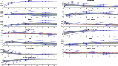
As studies have indicated that oil prices variable could possibly influence the results then in order to check for a possible omitted variables bias, I also try to specify a model with oil prices included, as in, for example, Baek and Miljkovic (2018). The results are presented in Figure 2 and they are very similar to the results of the benchmark model.

Figure 2. Impulse responses to policy rate and balance sheet shocks in Finland and the euro area with oil prices in the model (2009Q1-2018Q2). Notes: The area bordered by lines displays the impact of policy rate shocks, the shadowed area shows the impact of the balance sheet shocks (68% credible set). The line within a credible set represents the median of the impulse responses. * is used to mark the euro area variables, the other variables are the domestic variables of Finland.

6. Conclusion

As witnessed during the financial crises, the housing market can have an amplifying effect in the transmission of financial market disruptions into the real economy. This makes it important to see how different types of monetary policy would influence house prices.

In this paper, I study the effects of monetary policy shocks on house prices in Finland, a small open economy that is part of the euro area. Using a combination of zero and sign restrictions within the Bayesian SVAR framework, I identify two types of monetary policy shock, which are a policy rate shock and a balance sheet shock. A policy rate shock is identified as an exogenous innovation to the central bank’s policy interest rate and a balance sheet shock as an exogenous innovation to the central bank’s balance sheet that leaves the policy rate unchanged.

The results of the paper indicate that an expansionary policy rate shock has a small and positive impact on house prices in Finland and the whole euro area. In Finland the peak of the effect of a policy rate shock on house prices arrives faster than in the whole euro area and the effect is more persistent than in the euro area. However, the impacts peak at quite similar magnitude in both Finland and the euro area with the impact being a bit larger in case of Finland.

The impact of the balance sheet policies on house prices is very small in Finland, as is the impact on house prices in the euro area. The impacts are of the same magnitude. To the best of my knowledge, the impact of unconventional monetary policy on the house prices of an individual euro area country has not studied before. As there are a couple of papers that investigate the effect of unconventional monetary policy on house prices in the euro area (Huber & Punzi, 2020; Rahal, 2016), we can say that the results for the whole euro area obtained in my paper are similar to those of the few existing earlier studies.

The findings of the paper indicate that policy rate shocks have a larger and more persistent impact on house prices than balance sheet shocks do, both in the small euro area economy of Finland and in the euro area as a whole. In Finland though, the peak of the effect of a policy rate shock on house prices and on housing starts is reached faster than it is in the whole euro area, showing that the response of the housing market is faster in a small open economy than in the whole monetary union. The results of the paper may indicate that the impact of a conventional monetary policy shock on main economic indicators could be stronger and more persistent than the effect of an unconventional monetary policy shock in a monetary union.

In future studies, the impact of the two types of monetary policy shock on house prices could be studied in a larger set of individual euro area countries, with a focus on the sources of possible differences in the results across countries. It would also be pertinent to study in greater detail why conventional monetary policy tends to have a larger effect on macroeconomic variables than unconventional monetary policy does in the euro area. Another powerful alternative for future research is using narrative sign restrictions for the identification of shocks.

Acknowledgements

The author would like to thank the editor of the Baltic Journal of Economics Konstantins Benkovskis, two anonymous referees, Merike Kukk, Karsten Staehr, and Lenno Uusküla for their useful comments and suggestions. This work is partially supported by Doctoral School in Economics and Innovation, ASTRA project code 2014-2020.4.01.16-0032 (European Union, European Regional Development Fund). Declaration of interest: none.

Disclosure statement

No potential conflict of interest was reported by the author(s).

Notes on contributor

Signe Rosenberg is a doctoral student and works as a lecturer at Tallinn University of Technology.

Additional information

Funding

This work was supported by European Regional Development Fund [grant number 2014-2020.4.01.16-0032].

Notes

1 GDP, building permits and the central bank’s total assets are expressed per capita in order to ensure that changes in those variables are not affected by changes in population and to overcome the differences in scale between the euro area and Finland.

Appendices

Appendix A Description and Sources of the Data

Table

Variable	Description	Source
GDP*	GDP of the euro area at current prices divided by the population of the euro area.	Statistical Data Warehouse
HICP*	Harmonized index of consumer prices of the euro area.	Eurostat
House prices*	Residential property price index of the euro area.	National sources, BIS Residential Property Price database
Housing starts*	Building permits index of the euro area, square metres of useful floor area of all residential buildings excluding residences for communities divided by the population of the euro area.	Statistical Data Warehouse
Mortgage interest rate*	Loans to households for house purchases, over 10 years, new business coverage. Data were monthly, I calculated the quarterly averages.	Statistical Data Warehouse
Short term interest rate*	Euro overnight index average (EONIA). Data were monthly, I calculated the quarterly averages.	Eikon/ECB
Central bank’s total assets*	ECB total assets divided by the population of the euro area.	Eikon/ECB
GDP	GDP of Finland at current prices divided by the population of Finland.	Statistics Finland
HICP	Harmonized index of consumer prices of Finland.	Eurostat
House prices	House price index of Finland.	National sources, BIS Residential Property Price database
Housing starts	Building permits of residential buildings, square metres of floor area divided by the population of Finland. Data were monthly, I calculated the quarterly sums.	Statistics Finland
Mortgage interest rate	Loans to households for house purchases, over 5 years, outstanding loans. Data were monthly, I calculated the quarterly averages.	Statistical Data Warehouse
Oil prices*	Brent crude oil prices, converted into euros. Data were monthly, I calculated the quarterly averages.	Federal Reserve Bank of St. Louis

Note: The euro area variables are marked with *.

Appendix B Impulse responses with alternative measures for the short-term interest rate

Figure B1 Impulse responses to policy rate and balance sheet shocks using EURIBOR as a measure for the short-term interest rate. Notes: The area bordered by lines displays the impact of policy rate shocks, the shadowed area shows the impact of balance sheet shocks (68% credible set). The line within a credible set represents the median of impulse responses. * is used to mark the euro area variables, the other variables are the domestic variables of Finland.

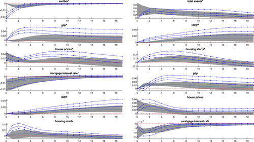
Figure B2 Impulse responses to policy rate and balance sheet shocks using MLF as a measure for the short-term interest rate. Notes: The area bordered by lines displays the impact of policy rate shocks, the shadowed area shows the impact of balance sheet shocks (68% credible set). The line within a credible set represents the median of impulse responses. * is used to mark the euro area variables, the other variables are the domestic variables of Finland.

Appendix C Time series for the identified shocks

Figure C1. Time series for a policy rate shock and a balance sheet shock.

Appendix D Impulse responses rescaled by the peak impact on euro area GDP

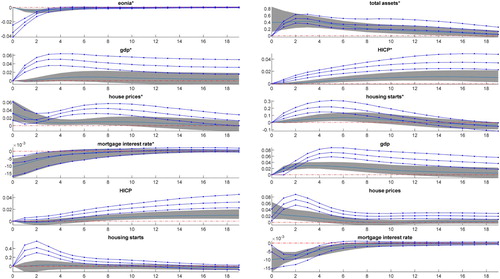
Figure D1 Impulse responses to policy rate and balance sheet shocks rescaled to yield the same impact on euro area GDP. Notes: The area bordered by lines displays the impact of policy rate shocks, the shadowed area shows the impact of balance sheet shocks (68% credible set). The line within a credible set represents the median of impulse responses. * is used to mark the euro area variables, the other variables are the domestic variables of Finland.

References

- Alessi, L., & Kerssenfischer, M. (2019). The response of asset prices to monetary policy shocks. Journal of Applied Econometrics, 34(5), 661–672. https://doi.org/10.1002/jae.2706
- Arias, J. E., Rubio-Ramirez, J. F., & Waggoner, D. F. (2018). Inference based on structural vector autoregressions identified with sign and zero restrictions: Theory and applications. Econometrica, 86(2), 685–720. https://doi.org/10.3982/ECTA14468
- Aspachs-Bracons, O., & Rabanal, P. (2011). The effects of housing prices and monetary policy in a Currency union. International Journal of Central Banking, 7(1), 225–274.
- Baek, J., & Miljkovic, D. (2018). Monetary policy and overshooting of oil prices in an open economy. The Quarterly Review of Economics and Finance, 70, 1–5. https://doi.org/10.1016/j.qref.2018.04.015
- Baumeister, C., & Benati, L. (2013). Unconventional monetary policy and the great recession: Estimating the macroeconomic effects of a spread compression at the zero lower bound. International Journal of Central Banking, 9(2), 165–212.
- Bernanke, B. S., & Kuttner, K. N. (2005). What explains the stock market’s reaction to Federal Reserve policy? The Journal of Finance, 60(3), 1221–1257. https://doi.org/10.1111/j.1540-6261.2005.00760.x
- Bjørnland, H. C., & Jacobsen, D. H. (2010). The role of house prices in the monetary policy transmission mechanism in small open economies. Journal of Financial Stability, 6(4), 218–229. https://doi.org/10.1016/j.jfs.2010.02.001
- Boeckx, J., Dossche, M., & Peersman, G. (2017). Effectiveness and transmission of the ECB’s balance sheet policies. International Journal of Central Banking, 13(1), 297–333.
- Bohl, M. T., Siklos, P. L., & Sondermann, D. (2008). European stock markets and the ECB’s monetary policy surprises. International Finance, 11(2), 117–130. https://doi.org/10.1111/j.1468-2362.2008.00219.x
- Calza, A., Monacelli, T., & Stracca, L. (2013). Housing finance and monetary policy. Journal of the European Economic Association, 11(S1), 101–122. https://doi.org/10.1111/j.1542-4774.2012.01095.x
- Cesa-Bianchi, A. (2013). Housing cycles and macroeconomic fluctuations: A global perspective. Journal of International Money and Finance, 37, 215–238. https://doi.org/10.1016/j.jimonfin.2013.06.004
- Cesa-Bianchi, A., Cespedes, L. F., & Rebucci, A. (2015). Global liquidity, house prices and the macroeconomy: Evidence from advanced and emerging economies. Journal of Money, Credit and Banking, 47(S1), 301–335. https://doi.org/10.1111/jmcb.12204
- Cesa-Bianchi, A., Ferrero, A., & Rebucci, A. (2018). International credit supply shocks. Journal of International Economics, 112, 219–237. https://doi.org/10.1016/j.jinteco.2017.11.006
- Christiano, L. J., & Eichenbaum, M. (2005). Nominal rigidities and the dynamic effects of a shock to monetary policy. Journal of Political Economy, 113(1), 1–45. https://doi.org/10.1086/426038
- Dieppe, A., Legrand, R., & van Roye, D. (2016). The BEAR Toolbox, ECB Working Paper Series, No. 1934.
- Elbourne, A., Ji, K., & Duijndam, S. (2018). The effects of unconventional monetary policy in the Euro Area, CPB Discussion Paper, No. 371.
- Errit, G., & Uusküla, L. (2014). Euro area monetary policy transmission in Estonia. Baltic Journal of Economics, 14(1–2), 55–77. https://doi.org/10.1080/1406099X.2014.980113
- Gabriel, S., & Lutz, C. (2017). The Impact of unconventional monetary policy on real estate market. mimeo. https://ssrn.com/abstract=2493873
- Gambacorta, L., Hofmann, B., & Peersman, G. (2014). The effectiveness of unconventional monetary policy at the zero lower bound: A cross-country analysis. Journal of Money, Credit and Banking, 46(4), 615–642. https://doi.org/10.1111/jmcb.12119
- Giuliodori, M. (2005). The role of house prices in the monetary transmission mechanism across European countries. Scottish Journal of Political Economy, 52(4), 519–543. https://doi.org/10.1111/j.1467-9485.2005.00354.x
- Gupta, R., & Jooste, C. (2018). Unconventional monetary policy shocks in OECD countries: How important is the extent of policy uncertainty. International Economics and Economic Policy, 15(3), 683–703. https://doi.org/10.1007/s10368-017-0380-8
- Huber, F., & Punzi, M. T. (2020). International housing markets, unconventional monetary policy and the zero lower bound. Macroeconomic Dynamics, 24(4), 774–806. https://doi.org/10.1017/S1365100518000494
- Kilian, L., & Lütkepohl, H. (2017). Structural vector autoregressive analysis, p. 782. Cambridge University Press.
- Mumtaz, H., & Surico, P. (2009). The transmission of international shocks: A factor-augmented VAR approach. Journal of Money, Credit and Banking, 41(S1), 71–100. https://doi.org/10.1111/j.1538-4616.2008.00199.x
- Nocera, A., & Roma, M. (2017). House prices and monetary policy in the euro area: Evidence from structural VARs, ECB Working Paper Series, No. 2073.
- Oikarinen, E. (2007). Studies on house price dynamics, Turku School of Economics, Series A-9: 2007.
- Oikarinen, E. (2009). Interaction between housing prices and household borrowing: The Finnish case. Journal of Banking & Finance, 33(4), 747–756. https://doi.org/10.1016/j.jbankfin.2008.11.004
- Peersman, G. (2011). Macroeconomic effects of unconventional monetary policy in the Euro Area, ECB Working Paper, No. 1397.
- Pesaran, M. H., & Smith, R. (1995). Estimating long-run relationships from dynamic heterogenous panels. Journal of Econometrics, 68(1), 79–113. https://doi.org/10.1016/0304-4076(94)01644-F
- Rahal, C. (2016). Housing markets and unconventional monetary policy. Journal of Housing Economics, 32(C), 67–80. https://doi.org/10.1016/j.jhe.2016.04.005
- Renzhi, N. (2018). House prices, inflation and unconventional monetary policy, Mimeo, available at SSRN: https://ssrn.com/abstract=3174289</objidref.
- Rigobon, R., & Sack, B. (2004). The impact of monetary policy on asset prices. Journal of Monetary Economics, 51(8), 1553–1575. https://doi.org/10.1016/j.jmoneco.2004.02.004
- Rosenberg, S. (2019). The effects of conventional and unconventional monetary policy on house prices in the Scandinavian countries. Journal of Housing Economics, 46, 1–17. https://doi.org/10.1016/j.jhe.2019.101659
- Schenkelberg, H., & Watzka, S. (2013). Real effects of quantitative easing at the zero lower bound: Structural VAR-based evidence from Japan. Journal of International Money and Finance, 33, 327–357. https://doi.org/10.1016/j.jimonfin.2012.11.020
- Sims, C. A., Stock, J. H., & Watson, M. W. (1990). Inference in linear models with some unit roots. Econometrica, 58(1), 113–144.
- Smith, A.L. (2014). House prices, heterogeneous banks and unconventional monetary policy options. The Federal Reserve Bank of Kansas City Research Working Papers, No. 14–12.
- Uhlig, H. (2005). What are the effects of monetary policy on output? Results from an agnostic identification procedure. Journal of Monetary Economics, 52(2), 381–419. https://doi.org/10.1016/j.jmoneco.2004.05.007
- Ume, E. (2018). The impact of monetary policy on housing market activity: An assessment using sign restrictions. Economic Modelling, 68, 23–31. https://doi.org/10.1016/j.econmod.2017.04.013
- Weale, M., & Wieladek, T. (2016). What are the macroeconomic effects of asset purchases? Journal of Monetary Economics, 79, 81–93. https://doi.org/10.1016/j.jmoneco.2016.03.010