Country-level effects of the ECB's expanded asset purchase programme

ABSTRACT

This paper evaluates the macroeconomic effects of the European Central Bank's (ECB) Expanded asset purchase programme (APP) on Latvia and other euro area jurisdictions and investigates the cross-border transmission mechanism. To that end, we employ two different vector autoregressive (VAR) models, namely a bilateral structural VAR with block exogeneity (BSVAR-BE) and a multi-country mixed cross-section global VAR with stochastic volatility (MCS-BGVAR-SV). We find that the APP had a limited and weakly significant impact on Latvia's output while the effect on inflation has been robust due to depreciation of the euro. Regarding other jurisdictions, results suggest that the ECB's asset purchases had a larger impact on industrial production in the countries where it drove down long-term interest rates the most via portfolio rebalancing channel. Despite that, our evidence suggests that the APP was mainly transmitted to inflation via exchange rate depreciation rather than through aggregate demand-driven shifts in the Phillips curve.

KEYWORDS:

• Asset purchase programme
• quantitative easing
• euro area
• GVAR
• SVAR
• Bayesian estimation

JEL CODES:

• C54
• E47
• E58
• F42

1. Introduction

Following the Great Recession, central banks in advanced economies introduced a number of unconventional monetary policy measures, such as quantitative easing (QE), because policy rates became constrained by their lower bounds and were no longer able to influence long-term interest rates and ultimately to stimulate output and increase inflation towards the target (Stone et al. (2011) and Bridges and Thomas (2012)). As one of the last major central banks, the European Central Bank announced the Asset Purchase Programme on 22 January 2015 to prevent the euro area economy from entering a deflationary spiral.¹ There is a burgeoning body of empirical literature documenting area-wide effects of the APP (see Altavilla et al. (2015), De Santis (2016) and Koijen et al. (2016) for the impact on the euro area financial conditions as well as Blattner and Joyce (2016), Garcia Pascual and Wieladek (2016) and Gambetti and Musso (2017) for the macroeconomic implications of the APP).

However, Georgiadis (2015) demonstrates that there is a significant heterogeneity in the transmission of conventional monetary policy shock among the euro area countries due to differences in structural properties of the member states. Some evidence regarding country-level effects of unconventional measures can be found in Boeckx et al. (2017) and Burriel and Galesi (2018), which confirm the results of Georgiadis (2015), but they focus on balance sheet policies implemented before the APP and use pre-APP data samples. Therefore, we expand the literature by focusing specifically on the member-state level transmission of the APP shock.² To make sure that we specifically identify the APP shock and disentangle it from previously introduced unconventional measures, our identification strategy explicitly emphasizes the portfolio rebalancing channel of asset purchases since the existing literature highlights its importance in the transmission of the APP shock in the euro area. However, the main aim of this paper is to evaluate the macroeconomic effects of the APP on the Latvian economy and investigate the cross-border transmission mechanism.³ To that end, we employ two different vector autoregressive models often used to evaluate the spillovers stemming from the foreign monetary policy actions, namely a bilateral structural VAR with block exogeneity and a multi-country mixed cross-section global VAR with stochastic volatility. While the first model provides a flexible framework for assessing the spillovers from monetary policy shocks in the euro area, the second framework allows to explicitly model Latvia as a member of the currency union and capture higher order transmission channels since the model also includes non-euro area countries, thus sharpening the estimates of the APP effects. Both models are estimated using Bayesian techniques with the data covering the period from January 2009 to October 2018 to minimize the vulnerability to the Lucas critique. Our contribution to the literature examining the effectiveness of the ECB's Asset Purchase Programme is threefold. First, we provide empirical evidence regarding the macroeconomic impact of the APP on the Latvian economy. Second, we present country-level results of the APP effectiveness. Third, the passage of time and the availability of longer time series allow us to empirically validate the area-wide total impact of the Asset Purchase Programme.

The paper is organized as follows. Section 2 describes the econometric models, data and identification strategy used to measure the impact of the APP. Section 3 presents the results and discusses the transmission mechanism, while Section 4 is devoted to robustness checks of our estimates. Finally, Section 5 concludes.

2. Econometric framework

This section describes the econometric strategy we use to pin down the impact of the APP on individual euro area jurisdictions. The first subsection introduces the bilateral SVAR which is specifically employed to evaluate the macroeconomic effects of the asset purchases on the Latvian economy, while the second subsection presents the multi-country VAR, which allows to explore the transmission of the APP on other member states and corroborate the findings regarding the Latvian economy.

2.1. Bayesian structural vector autoregression with block exogeneity

Bilateral VAR models with block exogeneity, first introduced by Cushman and Zha (1997), are frequently used to study monetary policy spillovers from large to small economies (see, e.g. Bluwstein and Canova (2015) and Moder (2017)) to foster a meaningful identification of shocks and ensure that shocks originating in a large economy can influence developments in a small economy but not vice versa.

Consider the following SVAR model:(1) $\begin{array}{c}{A}_0{x}_t=a_0+\sum _{j=1}^p{A}_j{x}_{t-j}+{\epsilon }_t\end{array}$(1) where $a_0$ is a vector of constants, $A_j$ is an m × m array of coefficients, $x_t$ for t = 1, … ,T is an m × 1 vector of m variables and ${\epsilon }_t$ is an m × 1 vector of residuals with variance-covariance matrix ${\mathrm{\Sigma }}_t$. In order to ensure that Latvian variables have no impact on the euro area block, we impose block exogeneity by making $A_j$ lower triangular:(2) $\begin{array}{c}{A}_j=\left[\begin{array}{cc}{A}_{11}^j& 0\\ A_{21}^j& A_{22}^j\end{array}\right],j=0,\dots ,p\end{array}$(2) In effect, the introduction of block exogeneity in the SVAR system implies that both impact matrix $A_0$ and coefficients $A_j$ with regard to Latvian variables in the euro area equations are forced to take a value of 0. Since we estimate our model using Bayesian methods, this is straightforward to implement by setting a 0 prior mean on the corresponding coefficients and by assigning hyper-parameter ${\lambda }_5,$ which controls the block exogenous variance, to take a value of 0.001, ensuring that the posterior distribution of these coefficients is centred tightly around 0. In this case, we use an independent normal-Wishart prior distribution, which assumes that the matrix containing VAR coefficients $A_j$ is multivariate normal:(3) $\begin{array}{c}{A}_j\sim N\left(A_{j_0},{\mathrm{\Omega }}_0\right)\end{array}$(3) where coefficient mean $A_{j_0}$ is an $m\times 1$ vector and ${\mathrm{\Omega }}_0$ is an m × m diagonal coefficient covariance matrix with variance relating endogenous variables to their own lags given by:(4) $\begin{array}{c}{\sigma }_{ii}^2={\left(\frac{{\lambda }_1}{l^{{\lambda }_3}}\right)}^2\end{array}$(4) where ${\lambda }_1$ is a hyper-parameter that controls the overall tightness, $l$ is the lag considered by the coefficient and ${\lambda }_3$ controls the relative tightness of the variance of lags other than the first one. The variance for cross-variable lag coefficients is given by:(5) $\begin{array}{c}{\sigma }_{ij}^2=\left(\frac{{\sigma }_i^2}{{\sigma }_j^2}\right){\left(\frac{{\lambda }_1{\lambda }_2}{l^{{\lambda }_3}}\right)}^2\end{array}$(5) where ${\sigma }_i^2$ and ${\sigma }_j^2$ denote the OLS residual variances of an autoregressive model estimated for variables $i$ and $j$ and ${\lambda }_2$ is a hyper-parameter that controls the cross-variable weighting. Finally, the variance for the constant is given by:(6) $\begin{array}{c}{\sigma }_c^2={\sigma }_i^2{\left({\lambda }_1{\lambda }_4\right)}^2\end{array}$(6) where ${\lambda }_4$ is a hyper-parameter governing the exogenous variable tightness. In our case, we specify the prior using standard values for the hyper-parameters following Dieppe et al. (2016), i.e. we set the AR coefficient of the prior to 0.8, overall tightness ${\lambda }_1=0.1$, cross-variable weighting ${\lambda }_2=0.5$ and lag decay ${\lambda }_3=1$. Turning to the prior for the residual covariance matrix $\mathrm{\Sigma }$, we assume that it follows an inverse Wishart distribution:(7) $\begin{array}{c}\mathrm{\Sigma }\sim IW\left(S_0,{\alpha }_0\right)\end{array}$(7) where $S_0$ is an $m\times m$ scale matrix for the prior and ${\alpha }_0$ is the number of degrees of freedom. $S_0$ is obtained from individual AR regressions following Karlsson (2012):(8) $\begin{array}{c}{S}_0=\left({\alpha }_0-m-1\right)\left(\begin{array}{cccc}{\sigma }_1^2& 0& 0& 0\\ 0& {\sigma }_2^2& 0& 0\\ 0& 0& \ddots & 0\\ 0& 0& 0& {\sigma }_m^2\end{array}\right)\end{array}$(8) where the degrees of freedom are set to ${\alpha }_0=m+2$.

Since no analytical solution exists for the independent normal-Wishart prior, we employ a Gibbs sampler to obtain the posterior distribution of the reduced form parameters and the residual covariance matrix with a total number of 12 000 iterations with the first 10 000 discarded as burn-in.

In our baseline specification of the model, the euro area block includes seven monthly variables: output, inflation, short-term and long-term interest rates, the exchange rate, equity prices and securities held by the Eurosystem, while the Latvian block – output, inflation and long-term interest rates (see Appendix A1). To pin down the transmission mechanism of the Eurosystem asset purchases to the Latvian economy, we further expand the model with additional variables one by one. The variables enter the model in form of log-levels with exception of interest rates which enter in levels. Expressing the variables as natural logarithms allows the results to be interpreted as elasticities, enabling us to estimate the total impact of the APP by scaling the impulse response functions. As for the sample period, we estimate the model with data covering the period from January 2009 to October 2018. Similarly to Boeckx et al. (2017), Gambetti and Musso (2017) and Burriel and Galesi (2018) we decide to use a data sample since the onset of the Great Recession to minimize the vulnerability to the Lucas critique. The lag order is set to 2.⁴

To identify the structural APP shock, we use the sign and zero restrictions approach as in Arias et al. (2014) with a summary of the identification scheme provided in Table 1. We choose an identification strategy similar to Garcia Pascual and Wieladek (2016) since the existing literature emphasizes the importance of the portfolio rebalancing channel in the transmission of the APP shock in the euro area (see, e.g. Altavilla et al. (2015), Gambetti and Musso (2017)), but instead of identifying the APP shock from the unobservable asset purchase announcement variable we use the balance sheet item "Securities held by the Eurosystem" as a proxy for the APP since this position is directly affected by asset purchases.

Table 1. Identification scheme in the BSVAR-BE model.

Shock	EA Industrial production	EA HICP inflation	Securities held by the Eurosystem	EA 10-year bond yields	EONIA	Eurostoxx 50	USD/EUR	LV Industrial production	LV HICP inflation	LV 10-year bond yields
Aggregate demand	+	+	0	+		+
Aggregate supply	+	–	0	+		+
Monetary policy	+	+	0		–
APP			+	–	0	+		0	0

We assume that the long-term interest rates decline in response to central bank asset purchases. This restriction is motivated by the evidence from Vayanos and Vila (2009), which shows quantitative easing can reduce the term premia of long-term bonds due to financial frictions. Additionally, Bernanke et al. (2004) argues that when a central bank performs asset purchases, it signals that inflation and output are far from their desired levels, meaning that short-term interest rates will stay low for a prolonged period, driving down long-term interest rates as well. Because of lower government bond yields, we believe that investors will try to compensate the fall in the return of their portfolios by rebalancing them to higher yielding assets, e.g. equities. We assume that, due to higher demand, equity prices will increase following the APP shock. However, we remain agnostic about the impact on the euro area output and inflation to let the data speak and impose a zero restriction on EONIA to reflect the zero lower bound environment and ensure that the APP shock is orthogonal to a conventional monetary policy shock. To further isolate the asset purchase shock from standard monetary policy actions, we also identify a conventional monetary policy shock.⁵ Finally, aggregate demand and supply shocks are also singled out so that disturbances related to business cycle fluctuations are not confused with the APP. Regarding the Latvian block of the model, we assume that real variables do not react immediately to asset purchases to disentangle the structural APP shock from domestic real economy disturbances as domestic demand and supply shocks are not explicitly identified. However, we leave the long-term interest rates unrestricted since Latvian bonds are also purchased under the APP. Sign restrictions are imposed to hold on impact and two months after, while zero restrictions – on impact only.

2.2. Mixed cross-section Bayesian global vector autoregression with stochastic volatility

A potential drawback of bilateral VARs is the lack of higher-order transmission channels which might lead to the underestimation of spillover effects (see Georgiadis (2017)). This encourages us to adopt a multi-country framework, namely the global vector autoregression first introduced by Pesaran et al. (2004), typically estimated with standard maximum likelihood techniques. However, given the large number of parameters to be estimated (up to six variables for each of the 34 countries included in our model) and relatively short time series (January 2009 – October 2018), estimation error is likely to be large, resulting in wide confidence bands. We choose to resolve the curse of dimensionality by introducing Bayesian shrinkage, thus creating a Bayesian GVAR in the spirit of Feldkircher and Huber (2016) and Crespo Cuaresma et al. (2016).⁶ The construction of the GVAR system is performed in two stages. The first step requires the estimation of the VARX* model for each country $i\in i=0,\dots ,N$:(9) $\begin{array}{c}{x}_{i,t}=a_{i,0}+\sum _{j=1}^p{\mathrm{\Phi }}_{i,j}{x}_{i,t-j}+\sum _{s=0}^q{\mathrm{\Lambda }}_{i,j}{x}_{i,t-s}^{\ast }+{\vartheta }_{i,0}{d}_t+{\vartheta }_{i,1}{d}_{t-1}+{\epsilon }_{i,t}\end{array}$(9) where $a_{i,0}$ is a vector of constants, $x_{i,t}$ is a $k_i\times 1$ vector of domestic variables and $x_{i,t}^{\ast }$ is a$k_i^{\ast }\times 1$ vector of weakly exogenous variables variables. ${\mathrm{\Phi }}_{i,j}$ and ${\mathrm{\Lambda }}_{i,j}$ are the coefficient matrices associated with domestic and weakly exogenous variables and $p$ and $q$ denote the lag order for domestic and weakly exogenous variables respectively. The weakly exogenous variables are calculated as cross-sectional weighted averages of other countries’ endogenous variables and allow us to capture the international linkages by using bilateral trade weights:(10) $\begin{array}{c}{x}_{i,t}^{\ast }=\sum _{j=0}^N{w}_{i,j}{x}_{j,t}\end{array}$(10) where $w_{i,j}$ denotes bilateral trade weights, $i$ is the country index and $j$ is the index of trading partner. Trade weights are constructed as follows:(11) $\begin{array}{c}{w}_{i,j}=\frac{{\sum }_{t=1}^N{T}_{i,j}}{{\sum }_{t=1}^N{T}_i}\end{array}$(11) where ${\sum }_{t=1}^N{T}_{i,j}$ denotes bilateral trade between countries $j$ and $i$ in period $t$, ${\sum }_{t=1}^{N}T$ is the total trade of country $i$ during the period $t$ and trade is calculated as:(12) $\begin{array}{c}{T}_{i,j}=\frac{Expor{t}_{i,j}+Impor{t}_{i,j}}{2}\end{array}$(12) Since we use a fixed weighting scheme, we average the weights over the period from 2009 to 2017.

Additionally, our model includes the $k^{ex}\times 1$ matrix of strictly exogenous variables with its corresponding coefficient matrix denoted by ${\vartheta }_i$.

In order to account for the common monetary policy in the euro area, we develop a mixed cross-section GVAR along the lines of Georgiadis (2015), but instead of modelling it in a univariate Taylor-rule type regression, we model the common monetary policy as a VAR-process. This cross-sectional unit, which we label "ECB", evolves according to:(13) $\begin{array}{c}{x}_{ECB,t}=a_{ECB,0}+\sum _{j=1}^p{D}_{ECB,j}{x}_{ECB,t-j}+\sum _{s=0}^q{F}_{ECB,j}{x}_{t-s}^{\ast }+{\epsilon }_{ECB,t}\end{array}$(13) where $x_{ECB,t}$ is a vector of common euro area variables, i.e. EONIA, securities held by the Eurosystem, the exchange rate of the euro against the US dollar and Eurostoxx 50⁷ and $x_t^{\ast }$ is a vector of PPP-GDP weighted averages of output and inflation of the euro area member states.⁸ Oil prices are also modelled in a similar fashion, following Chudik and Pesaran (2013), who proposes to include them as a dominant unit rather than to endogenously determine them within the US country model:(14) $\begin{array}{c}{x}_{OIL,t}=a_{OIL,0}+\sum _{j=1}^p{\mathrm{\Phi }}_{OIL,j}{x}_{OIL,t-j}+\sum _{s=0}^q{\mathrm{\Lambda }}_{OIL,j}{x}_{t-s}^{\ast }+{\epsilon }_{OIL,t}\end{array}$(14) where $x^{\ast }$ is a vector of PPP-GDP weighted average of output of all countries included in the GVAR to mimic the demand for oil.

Since the data sample includes several episodes of severe economic volatility (e.g. the Great Recession, euro area debt crisis and introduction of non-standard monetary measures), we introduce stochastic volatility in our GVAR by allowing variance-covariance matrix ${\mathrm{\Sigma }}_{i,t}$ of the error term ${\epsilon }_{i,t}$ to change over time:(15) $\begin{array}{c}{\epsilon }_{i,t}\sim N\left(0,{\mathrm{\Sigma }}_{i,t}\right),\end{array}$(15) $\begin{array}{c}{\mathrm{\Sigma }}_{i,t}=U_i{H}_{i,t}{U}_i^{\mathrm{\prime }}\end{array}$where $U_i$ is a lower triangular matrix with a unit diagonal and off-diagonal elements $u_{ij,n}$ $(j=2,\dots ,k_i$and $n=1,\dots ,j-1)$ and $H_{i,t}$ is a diagonal matrix of log-volatilities denoted by $h_{ij,t}$which follow an AR(1) process:(16) $\begin{array}{c}{h}_{ij,t}={\mu }_{ij}+{\rho }_{ij}\left(h_{ij,t-1}-{\mu }_{ij}\right)+k_{ij,t}\end{array}$(16) where ${\mu }_{ij}$ is the mean of log-volatility, ${\rho }_{ij}$ is the persistence parameter and $k_{ij,t}$ is a white noise error.

After estimating the VARX* model for each country, in the second stage we stack them in a single system to yield a global vector autoregression:(17) $\begin{array}{c}G{x}_t=a_0+\sum _{n=1}^{p^{\ast }}{F}_n{x}_{t-n}+{\vartheta }_0{d}_t+{\vartheta }_1{d}_{t-1}+{\epsilon }_{i,t}\end{array}$(17) where $x_t$ is a vector containing all endogenous variables of the system, $G$ is a $k\times k$ matrix of contemporaneous coefficients that are a function of the matrices associated with weakly exogenous variables ${\mathrm{\Lambda }}_{i,j}$ and weights $w_{i,j}$. Similarly, $F_n$ are $k\times k$ matrices of autoregressive coefficients that are a function of the matrices associated with endogenous variables ${\mathrm{\Phi }}_{i,j}$ and weights $w_{i,j}$ and$p^{\ast }$ denotes max(p, q). ${\epsilon }_{i,t}$ is a vector containing the residuals with their variances given by a block-diagonal matrix ${\mathrm{\Sigma }}_{i,t}=bdiag\left({\mathrm{\Sigma }}_{0,t},\dots ,{\mathrm{\Sigma }}_{N,t}\right)$. Multiplying with the inverse of matrix $G$ from the left gives the reduced-form of global vector autoregression:(18) $\begin{array}{c}{x}_t=G^{-1}{a}_0+G^{-1}\sum _{n=1}^{p^{\ast }}{F}_n{x}_{t-n}+G^{-1}{\vartheta }_0{d}_t+G^{-1}{\vartheta }_1{d}_{t-1}+G^{-1}{\epsilon }_t\end{array}$(18) By construction, the GVAR framework already involves a form of parameter reduction by restricting the coefficient matrices of weakly exogenous variables in large part to be defined by weights. However, given the relatively short time series, the remaining number of parameters is still too high for precise estimates. Therefore, we estimate our model with Bayesian methods by specifying the stochastic search variable selection (SSVS) prior as in Feldkircher and Huber (2016) and Crespo Cuaresma et al. (2016) for each country model. For convenience, suppose that we stack matrices of coefficients from equation 9(9) $\begin{array}{c}{x}_{i,t}=a_{i,0}+\sum _{j=1}^p{\mathrm{\Phi }}_{i,j}{x}_{i,t-j}+\sum _{s=0}^q{\mathrm{\Lambda }}_{i,j}{x}_{i,t-s}^{\ast }+{\vartheta }_{i,0}{d}_t+{\vartheta }_{i,1}{d}_{t-1}+{\epsilon }_{i,t}\end{array}$(9) for each country $i$ into vector ${\mathrm{\Psi }}_i=(a_{i,0}^{\mathrm{\prime }},vec{\left({\mathrm{\Phi }}_i\right)}^{\mathrm{\prime }},vec{\left({\mathrm{\Lambda }}_i\right)}^{\mathrm{\prime }},vec{\left({\vartheta }_{i,0}\right)}^{\mathrm{\prime }}vec{\left({\vartheta }_{i,1}\right)}^{\mathrm{\prime }}{)}^{\mathrm{\prime }}$. The advantage of the SSVS prior is that it reduces subjectivity regarding the variable selection for each country model in contrast to maximum likelihood GVARs. It is achieved by shrinking "unimportant" or small parameters to zero, thus ensuring that cross-country heterogeneities are taken into account. The prior is implemented as follows:(19) $\begin{array}{c}{\mathrm{\Psi }}_{ij}|{\delta }_{ij}\sim {\delta }_{ij}\mathrm{N}(0,{\tau }_{ij,0}^2)+(1-{\delta }_{ij}\left)\mathrm{N}\right(0,{\tau }_{ij,1}^2)\end{array}$(19) where ${\delta }_{ij}$ is a binary random variable corresponding to the variable$j$ in country model $i$. It takes the values of 1 in case the variable is included in the model and zero otherwise. The variable selection is governed by the hyper-parameters ${\tau }_{ij,0}$ and ${\tau }_{ij,1}$which we set in a semi-automatic fashion following George et al. (2008). Hyper-parameter ${\tau }_{ij,0}^2$ is applied to small coefficients with a value typically set close to zero to ensure that the posterior estimate of these coefficients is pushed close to zero, effectively excluding the variables with small coefficients from the model. For the remaining coefficients, hyper-parameter ${\tau }_{ij,1}^2$ is applied with relatively large values to ensure that the prior on these coefficients is non-informative, i.e. posterior estimate converges to the OLS estimates, ensuring that the results are not driven by subjectively specified prior information. In our setting, we specify ${\tau }_{ij,0}^2=0.1{\sigma }_j$ and ${\tau }_{ij,1}^2=3{\sigma }_j$ where ${\sigma }_j$ is the standard error for coefficient $j$ from each country's VARX* model estimated with OLS, allowing us to scale the hyperparameters for individual models. Given that our GVAR setup features stochastic volatility, we also impose a SSVS prior on the off-diagonal elements of $U_i$:(20) $\begin{array}{c}{u}_{ij,n}|{\kappa }_{ij,n}\sim {\kappa }_{ij,n}\mathrm{N}(0,{\varphi }_{ij,n0}^2)+(1-{\kappa }_{ij,n}\left)\mathrm{N}\right(0,{\varphi }_{ij,n1}^2)\end{array}$(20) where ${\kappa }_{ij,n}$ is a binary variable similar to ${\delta }_{ij}$ with the values of 1 in case the variable is included in the model and zero otherwise while ${\varphi }_{ij,n0}^2$ and ${\varphi }_{ij,n1}^2$ are hyper-parameters associated with the covariance matrix. We specify ${\varphi }_{ij,n0}^2=7$ and ${\varphi }_{ij,n1}^2=0.1$ for all $i,j,n.$

Estimation of the Bayesian variant of global vector autoregression requires the use of Markov Chain Monte Carlo (MCMC) methods. The algorithm can be summarized as follows: stacked coefficients from country models ${\mathrm{\Psi }}_{i,j}$ are drawn from the multivariate normal distribution, while ${\delta }_{ij}$ and ${\kappa }_{ij,n}$ are sampled from Bernoulli distribution. Finally, time-varying variance-covariance matrix ${\mathrm{\Sigma }}_{i,t}$ of the error term ${\epsilon }_{i,t}$ is simulated using the algorithm of Kastner and Frühwirth-Schnatter (2014).⁹ We obtain posterior estimates from 20 000 MCMC iterations after the first 20 000 draws have been discarded as burn-in.¹⁰

To identify the APP shock we use the sign restrictions approach as proposed by Eickmeier and Ng (2015), which applies algorithms of Arias et al. (2014) and Fry and Pagan (2011) to global vector autoregressions. It consists of applying the Cholesky decomposition to variance-covariance matrix ${\mathrm{\Sigma }}_{i,t}$ of the error term ${\epsilon }_{i,t}$ for each country model to obtain the lower triangular Cholesky matrix $P_i$. To perform impulse response analysis, it is necessary to construct $k\times k$ matrix P:(21) $\begin{array}{c}P=\left(\begin{array}{ccccc}{P}_0& 0& \dots & \dots & 0\\ 0& \ddots & & & ⋮\\ ⋮& & P_i& & ⋮\\ ⋮& & & \ddots & 0\\ 0& \dots & \dots & 0& P_N\end{array}\right)\end{array}$(21) The ECB and euro area country models differ from the rest because their structural errors $v_{i,t}=P_i{\epsilon }_{i,t}$ are then multiplied by randomly drawn $k_i\times k_i$ orthonormal rotation matrices $R_i$ from which we select candidate rotations that generate impulse responses satisfying the sign restrictions. The advantage of this approach is that the impulse response functions do not depend on the ordering of the countries and variables since the variance-covariance matrix is orthogonalized only in the countries where the shocks are identified. We use an identification scheme similar to the one used in the BSVAR-BE model with a summary of the identification scheme provided in Table 2.

Table 2. Identification scheme in the MCS-BGVAR-SV model.

Shock	Industrial production	HICP inflation	Securities held by the Eurosystem	10-year bond yields	EONIA	Eurostoxx 50	USD/EUR
Aggregate demand	+*	+*		+*		+
Aggregate supply	+*	–*		+*		+
APP			+	–*		+

The restrictions marked with * are imposed in the euro area country models and are only required to be fulfilled by the majority of member states, allowing for cross-country heterogeneity. The remaining restrictions are applied in the ECB model.

However, we are forced to impose a slightly smaller set of restrictions and drop the identification of the standard monetary policy shock since the algorithm of Eickmeier and Ng (2015) is computionally intensive due to the large orthogonal rotation matrix. Despite using weaker identification restrictions, the APP shock seems well identified and is not confused with standard monetary policy actions because the reaction of EONIA is statistically insignificant throughout the horizon as shown by the results in Figure 2.

Our monthly dataset is comprised of the main macroeconomic variables for 34 countries over the same period as the BSVAR-BE model, i.e. from January 2009 to October 2018. For non-euro area countries we include six endogenous variables, such as industrial production, inflation, long-term and short-term interest rates, the exchange rate and equity prices, while for the euro area countries we include the former three variables (see Appendix A2). The euro area monetary policy and common variables are modelled in a separate block labelled "ECB", which includes EONIA, securities held by the Eurosystem, the exchange rate of the euro against the U.S dollar and Eurostoxx 50. See Appendix A3 for a detailed specification of each country model.

3. Results

We start our analysis of the APP impact by examining the area-wide impulse responses to validate our identification scheme. Figure 1 shows the impulse response functions of the euro area macroeconomic variables from the BSVAR-BE model, while Figure 2 – from the MCS-BGVAR-SV model.

Figure 1. BSVAR-BE results for the euro area.

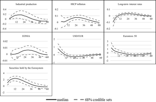
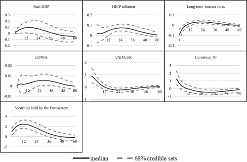
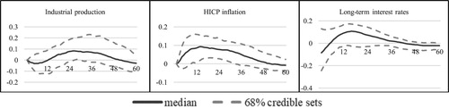
Figure 2. MCS-BGVAR-SV results for the euro area.

Note: Euro area results are estimated by aggregating impulse response functions of the member states using PPP-GDP weights.

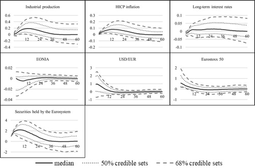
The APP shock is scaled to yield a 1 pp increase in the Eurosystem asset holdings as a fraction of the 2015 nominal GDP. The vertical axis is expressed in percent, while the horizontal axis shows the number of months since the shock. In general, both the shape of the impulse response functions and the estimated impact from both models are broadly similar, e.g. the estimated peak impact on industrial production from bilateral VAR is 0.17%, while the multi-country VAR, as intuitively expected, yields a slightly more pronounced reaction at 0.185% as this model also allows to capture spillback effects from the rest of the world. Considering that the Eurosystem asset holdings have increased by 21 pp relative to the 2015 nominal GDP from March 2015 to October 2018, we can scale the peak responses of the industrial production to conclude that the cumulative impact of the APP on the euro area output is about 3.6% – 3.9%. More importantly, both models show that inflation also received a considerable boost since its impulse response functions demonstrate that the asset purchase shock worth 1% of nominal GDP increased it by approximately 0.07–0.08 pp.

Thus, we can conclude that the APP was successful in reviving the inflationary pressures in the euro area since the rate of inflation would have been ∼ 1.5–1.7 pp lower in the case without the Eurosystem asset purchases. Comparing our results with the ECB staff estimates (see Hartmann and Smets 2018), which are based on a range of models, we can conclude that our estimate regarding the impact on inflation is identical, while the effect on output is somewhat higher due to the fact that we use industrial production instead of real GDP as a measure of output which is known to be more responsive to monetary shocks (Gambacorta et al. 2014).

Regarding the transmission mechanism, both models bring statistically significant evidence to the existence of portfolio rebalancing channel since sovereign bond yields decline and equity prices rise following the APP shock. The estimated elasticities of these variables are both qualitatively and quantitatively in line with the evidence found in Garcia Pascual and Wieladek (2016) as well as Gambetti and Musso (2017). Additionally, we find that the exchange rate channel was also activated since our estimates show that the euro depreciated by 15% – 19% against the US dollar – broadly in line with previous research. In general, the estimated elasticities of the euro area macroeconomic and financial variables to the asset purchase shock are in line with the previous literature, suggesting that the APP shock is well identified which is essential to further analyze country-level effects.

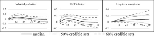
We start our analysis of member-state level effectiveness of the APP by focusing on the Latvian economy. Figure 3 shows the results from the bilateral VAR, while the results from the global VAR are found in Figure 4. The results from both models suggest that the APP has had a rather limited impact on Latvian output because the impulse response of the industrial production is only statistically significant at 50% level in the case of multi-lateral model, likely reflecting the importance of spillovers from non-euro area countries in the transmission of the APP to the Latvian economy.

Figure 3. BSVAR-BE results for Latvia.

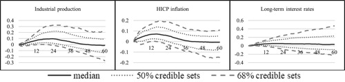
Figure 4. MCS-BGVAR-SV results for Latvia (total impact).

Still, the estimated cumulative effect on Latvian output at ∼ 2% is much smaller than the euro area average and contrasts the findings in the existing literature, which often estimates the real effects in Latvia from the ECB monetary policy to be among the highest in the euro area. A possible explanation is that these studies include data samples from the period before the Great Recession when Latvia experienced an excessive boom–bust cycle, and it is possible that some of these dynamics are misidentified with the ECB monetary policy.

However, the evidence from both models points to a robust impact on Latvian inflation as the impulse response functions of the HICP inflation are statistically significant at 68% level. Also the cumulative impact is similar to the euro area average as it would have been some 1.5–1.8 pp lower without the APP. The global VAR framework also allows us to estimate the direct impact of asset purchases by setting the bilateral trade weights between Latvia and other countries equal to zero, effectively switching off the spillovers from the euro area and the rest of the world. The results in Figure 5 show that indeed the effect on output was mostly generated by spillovers from other countries as the direct cumulative impact on the industrial production is around 0.7%. On the other hand, the direct impact on inflation remains strong at 1.1 pp cumulatively, suggesting that it was impacted by the APP-induced depreciation of the euro rather than through aggregate demand-driven shifts in the Phillips curve.

Figure 5. MCS-BGVAR-SV results for Latvia (direct impact).

With regard to the transmission channels, the baseline specification of both models shows that the portfolio rebalancing channel was not activated in the case of Latvia since the impulse responses of the long-term interest rate are not statistically significant. Therefore, to pin down the transmission mechanism, we expand the baseline specification of both models with additional variables one by one and leave them unrestricted to remain agnostic about the channels through which the asset purchases were transmitted to the real economy.

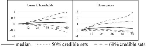
Figures 6 and 7 demonstrate that the financial channel was also not significant in the transmission of the APP to the Latvian economy because the responses of credit variables are statistically insignificant throughout the horizon. Accordingly, there is also weak evidence that the APP impacted house prices because only the response from the MCS-BGVAR-SV model is slightly significant at 50% level.

Figure 6. BSVAR-BE results: the financial channel.

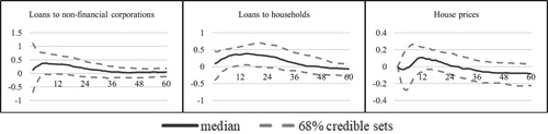
Figure 7. MCS-BGVAR-SV results: the financial channel.

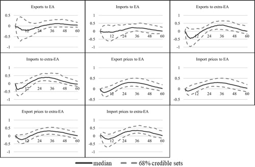
Next, we focus on various trade-specific variables with the results shown in Figure 8. Evidence supports our hypothesis that the APP caused higher consumer prices in Latvia due to the depreciation of the euro because import prices went up following the asset purchase shock, as expected from the theory. Since prices of imported intermediate goods increase, exporters are forced to increase their prices as well. While the response of exports to extra-EA suggest that despite the increase in export prices there was higher demand for Latvian goods from the rest of the world, extra-EA imports increased to a similar extent, thus leading to negligible impact on net exports. This helps to explain why the APP had a limited and statistically weakly significant impact on Latvian output.

Figure 8. BSVAR-BE results: the trade channel.

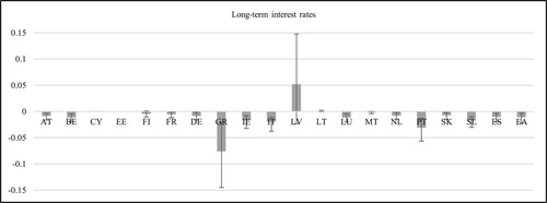
Finally, we now turn to member-state level transmission of the APP since the use of the MCS-BGVAR-SV model allows us to measure the impact of the common monetary policy across individual euro area jurisdictions. Figures 9 and 10 demonstrate that the APP had a larger impact on output in the countries where portfolio rebalancing was activated, i.e. where sovereign yields were depressed the most, in line with the findings of De Santis (2016). Regarding Latvia and the Baltics in general, our findings show that the APP effect on output was among the lowest in the euro area.

Figure 9. MCS-BGVAR-SV country-level results: output.¹¹

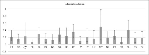
Figure 10. MCS-BGVAR-SV country-level results: sovereign yields.

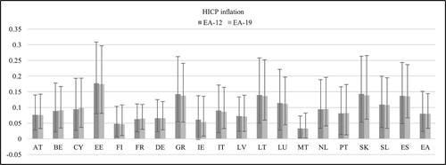
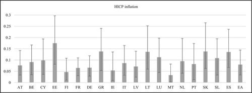
Figure 11 supports our argument that the Eurosystem's asset purchases affected inflation through the exchange rate channel rather than through aggregate demand-driven shifts in the Phillips curve since the countries with the largest impact on output not necessarily saw the largest increase in consumer prices. This finding is in line with the recent evidence of Beck et al. (2019), which studies the general experience of countries which have embarked on central bank asset purchases.

Figure 11. MCS-BGVAR-SV country-level results: inflation.

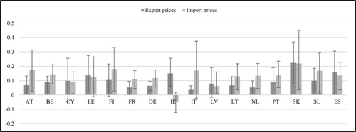
Regarding other transmission channels, Figure A1 in the Appendix shows that in some jurisdictions the financial channel was also activated as the APP enhanced lending to households and, subsequently, contributed to higher real estate prices. Figures A2 to A5 show that the APP-induced depreciation of the euro exchange rate did not lead to export-driven growth since the effect on net exports in most member states is negligible because imports also increase following the APP shock likely reflecting the boost in aggregate demand from the asset purchases transmitted through other channels. The reactions of import prices bring additional evidence to our hypothesis about the importance of the exchange rate channel in the transmission of the APP to consumer prices since higher import prices in most jurisdictions helped to revive inflationary pressures by essentially "importing" inflation from the rest of the world.

4. Sensitivity analysis

In this section of the paper we undertake a number of robustness checks. We start by investigating sensitivity of the results emanating from the BSVAR-BE model. First, we replace industrial production with real GDP as a measure of output in the euro area block so that our estimates of area-wide effectiveness of the APP are fully comparable with previous studies.

Figure 12 shows that, when using real GDP as measure of output, the shape of impulse response is almost identical to the baseline results, but, as expected, the estimated impact is much smaller as real GDP increases by 0.09% following a 1pp increase in the Eurosystem asset holdings relative to nominal GDP. This helps to bring the cumulative impact on output in line with the ECB staff estimates at approximately 2%, while the effect on inflation remains unchanged, suggesting that our identification strategy effectively isolates the APP shock.

Figure 12. Robustness check I: real GDP as measure of output.

To bring additional evidence showing that our identification scheme specifically identifies the APP shock and disentangles it from previously introduced unconventional measures, we compare the time series of the estimated shock with the one identified using the scheme à la Boeckx et al. (2017) and Burriel and Galesi (2018), utilizing our BSVAR-BE model. In this case, we replace the balance sheet item "Securities held by the Eurosystem" with the total assets, drop the equity prices, EONIA and euro area long-term interest rates and add the CISS index, MRO rate and its spread with EONIA.

The set of sign restrictions shown in Table 3 is imposed on impact and one month after the shock, while zero restrictions – on impact only. Figure 13 demonstrates that our identification strategy is more appropriate for recovering the APP shock since it correctly identifies the start of purchases in March 2015 (denoted with vertical line) and the recalibrations announced later on. The shock series before the launch of the APP is also much smoother than in the case when we use a competing identification strategy, indicating that our estimates of the asset purchases are safeguarded from the effects of balance sheet policies used before.

Figure 13. Robustness check II: comparison of the shock time series.

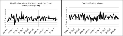
Table 3. Identification scheme à la Boeckx et al. (2017) and Burriel and Galesi (2018).

Shock	EA Industrial production	EA HICP inflation	Total assets of the Eurosystem	CISS index	MRO	EONIA-MRO spread	USD/EUR	LV Industrial production	LV HICP inflation	LV 10-year bond yields
Monetary policy	+	+	0		–
APP	0	0	+	–	0	–

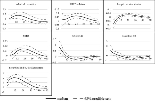
We double-check this by estimating the BSVAR-BE model using a pre-APP data sample. The results in Figure 14 confirm that our estimates are not confused with the non-standard monetary policy instruments implemented prior to the APP because both the response of output and inflation are small and statistically insignificant, indicating that the estimated APP effects are indeed coming from the period when the asset purchases were actually implemented. As an additional robustness check of the identifying restrictions employed in the BSVAR-BE model, we put a positive restriction on equity prices for the MP shock to disentangle pure monetary policy shock from news shocks, as argued in Jarociński and Karadi (2020). The responses to the APP shock reported in Figure 15 are almost unchanged from the baseline results, suggesting that they are not affected by a potentially misidentified standard monetary policy shock due to contamination from the central bank information shocks. Figure 16 shows that the results remain robust also when using MRO rate instead of the EONIA as a proxy for standard monetary policy actions.

Figure 14. Robustness check III: using a pre-APP data sample (January 2009 – August 2014).

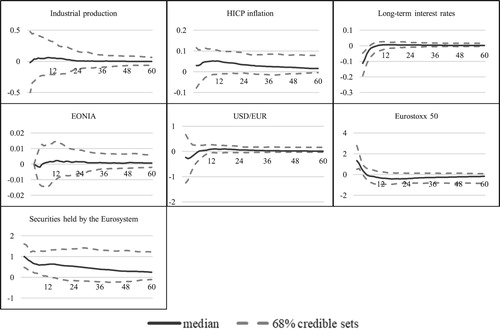
Figure 15. Robustness check IV: controlling for the central bank information shocks.

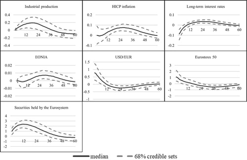
Figure 16. Robustness check V: using MRO rate as a proxy for standard monetary policy actions.

Next, we make sure that the estimated impact on the Latvian economy is not confused with country-specific business cycle dynamics by identifying aggregate demand and supply shocks also in the LV block as shown in Table 4.

Table 4. Identification scheme with LV-specific shocks.

Shock	EA Industrial production	EA HICP inflation	Securities held by the Eurosystem	EA 10-year bond yields	EONIA	Eurostoxx 50	USD/EUR	LV Industrial production	LV HICP inflation	LV 10-year bond yields
Aggregate demand	+	+	0	+		+
Aggregate supply	+	–	0	+		+
Monetary policy	+	+	0		–
APP			+	–	0	+		0	0
LV aggregate demand			0					+	+
LV aggregate supply			0					+	–

The results in Figure 17 show that the responses of Latvian variables to the APP disturbance are almost the same as in the baseline specification of the BSVAR-BE model meaning that they are isolated from domestic demand or supply shocks.

Figure 17. Robustness check VI: identifying LV-specific shocks.

Finally, we check the robustness of the MCS-BGVAR-SV model by assuming that common variables in the "ECB" model evolve according to PPP-GDP weighted dynamics of EA-12 output and inflation, instead of EA-19, since not all countries were members of the euro area in 2009 when our data sample starts. Figures A6 to A8 in the Appendix demonstrate that even when assuming that the euro area consists of EA-12, the impact of the APP remains virtually unchanged both in the countries that initially adopted the euro and in those that joined the currency union afterwards.

5. Conclusions

Our results suggest that the APP has had a limited and weakly significant impact on Latvia's output with the effect being among the lowest in the euro area, contrary to the existing literature, which evaluates the spillovers from the ECB monetary policy to the Latvian economy. Additionally, the evidence suggests that most of the impact on output was indirectly transmitted through other countries. However, our findings point to a robust impact on Latvian inflation with the magnitude being in line with the euro area average. The APP was transmitted to Latvian consumer prices via the exchange rate channel as the APP-induced depreciation of the euro caused higher import prices. Regarding other jurisdictions, we find that the ECB's asset purchases had a larger impact on output in the countries where the portfolio rebalancing channel was activated, i.e. where sovereign yields were depressed the most. Results show that in some countries the financial channel was also actuated as the APP enhanced lending and, subsequently, contributed to higher real estate prices. Nonetheless, it seems that asset purchases mainly affected inflation in other member states also via the exchange rate channel rather than through aggregate demand-driven shifts in the Phillips curve since the countries with the largest impact on output not necessarily saw the largest increase in consumer prices. Despite a significant depreciation of the euro following the introduction of asset purchases, there is very little evidence to suggest that they caused beggar-thy-neighbour-style side effects since the effect on net exports in most member states is negligible because imports also increase following the APP shock likely reflecting the boost in aggregate demand from the asset purchases transmitted through other channels.

The empirical findings reported in this paper also have important implications for the future monetary policy making in the euro area. Given the low interest rate environment, policy rates are likely to hit the effective lower bound more often, limiting the scope of conventional monetary policy tools to influence macroeconomic developments and ensure price stability. Thus, asset purchases will likely be used as the main monetary policy measure to fight adverse shocks and help steer inflation towards the target. While our results show that central bank asset purchases have very heterogenous effects among the individual euro area jurisdictions, the effects on inflation in all member states are significant nonetheless. Also our finding that asset purchases generate larger real effects in jurisdictions where they drive down sovereign yields the most suggest that asset purchases is an effective measure to eliminate financial fragmentation risks and ensure smooth transmission of common monetary policy stance to all euro area member states.

Acknowledgement

The author would like to thank participants of an internal seminar held at Latvijas Banka, the 10th Nordic Econometric Meeting, the 2nd Baltic Economic Conference and the 22nd Central Bank Macroeconomic Workshop for useful suggestions. Comments by three anonymous reviewers as well as Yannick Lucotte (Université d'Orléans) and Martin Feldkircher (Oesterreichische Nationalbank) are gratefully acknowledged. The views expressed in this paper are those of the author and do not necessarily reflect the views of Bank of Latvia.

Disclosure statement

No potential conflict of interest was reported by the author(s).

Notes on contributor

Andrejs Zlobins is a research economist at Bank of Latvia. His research interests include monetary and international economics, particularly the study of non-standard monetary policy tools and their spillovers.

Notes

1 See https://www.ecb.europa.eu/mopo/implement/omt/html/index.en.html for a detailed description of the APP.

2 Feldkircher et al. (2020) specifically look at the APP and model the euro area at a country level, but they are focusing on spillovers to the CESEE and non-euro area EU countries and don't report euro area country results.

3 The existing literature finds large real effects in Latvia (and the Baltics in general) from the ECB monetary policy (see Georgiadis (2015) for the evidence regarding conventional monetary policy shocks, Burriel and Galesi (2018) for unconventional monetary policy shocks and Benecká et al. (2018) for monetary policy shocks generally).

4 The use of rather parsimonious lag structure is motivated by the highly computationally intensive process of estimating the MCS-BGVAR-SV model, rendering higher lag order infeasible. To improve the comparability of models, we use the same lag order also in the BSVAR-BE model.

5 Please note that the balance sheet item "Securities held by the Eurosystem" do not include collateral banks have to deposit at the Eurosystem in order to borrow money within open market operations (these are reflected in balance sheet item "Lending to euro area credit institutions related to monetary policy operations denominated in euro"). Otherwise the zero restriction in case of the standard monetary policy shock would be violated.

6 I thank Martin Feldkircher for providing the programme code and helpful comments.

7 We use Eurostoxx 50 rather than national equity price indices to facilitate the number of successful rotation matrices that satisfy the sign restrictions during the impulse response analysis.

8 We assume that the euro area consists of EA-19.

9 See Feldkircher et al. (2020) and Feldkircher and Huber (2016) for technical information regarding the implementation of stochastic volatility and simulation of posterior.

10 Due to computational reasons and to further reduce the possibility of autocorrelation between the Markov chains, we use a thinning interval of 0.1 to save 2000 out of 20000 draws. To reduce the risk that our results are estimated from unstable draws, we exclude the iterations with large eigenvalues of the companion matrix, arriving at approximately 1500 draws from which the posterior is obtained.

11 Figure shows the peak responses along with whiskers denoting the corresponding 50% credible sets due to space considerations. Full set of impulse responses are available upon request. Note that the use of less stringent confidence intervals is not uncommon in empirical multi-country models (see e.g. Chudik and Fratzscher (2012), Almansour et al. (2015)).

Appendix

A1. BSVAR-BE dataset description and transformations

Table

Block	Variable	Description	Transformation	Data source
Baseline model	ipi	Seasonally adjusted industrial production index, 2010 = 100.	ln	Eurostat
	cpi	Seasonally adjusted annual rate of change in all-items consumer price index.	Levels	Eurostat
	sec	Securities of euro area residents denominated in euro held by the Eurosystem scaled by 2015 nominal GDP.	ln	Author's calculations based on the ECB and Eurostat data
	ltr	10-year government benchmark bond yields for the euro area. EMU convergence criterion bond yields for Latvia.	Levels	ECB, Eurostat
	eastr	EONIA.	Levels	ECB
	eaep	Dow Jones Euro Stoxx Price Index.	ln	ECB
	eaex	Monthly average value of the euro per US dollar.	ln	IMF IFS
Financial channel	cred_nfc	Loans to non-financial corporations. Outstanding amounts at the end of the period (stocks), total maturity.	ln	ECB
	cred_hh	Loans to households and NPISHs. Outstanding amounts at the end of the period (stocks), total maturity.	ln	ECB
	hp	Real residential property prices, 2010 = 100. Monthly series are obtained by performing the Chow-Lin temporal disaggregation procedure.	ln	BIS
Trade channel	exp_ea	Exports to the euro area. All products volume index, 2010 = 100.	ln	Eurostat
	exp_extra_ea	Exports to the extra-euro area. All products volume index, 2010 = 100.	ln	Eurostat
	imp_ea	Imports to the euro area. All products volume index, 2010 = 100.	ln	Eurostat
	imp_extra_ea	Imports to the extra-euro area. All products volume index, 2010 = 100.	ln	Eurostat
	euvi_ea	Export prices to the euro area. Unit value index, 2010 = 100.	ln	Eurostat
	euvi_extra_ea	Export prices to the extra-euro area. Unit value index, 2010 = 100.	ln	Eurostat
	iuvi_ea	Import prices to the euro area. Unit value index, 2010 = 100.	ln	Eurostat
	iuvi_extra_ea	Import prices to the extra-euro area. Unit value index, 2010 = 100.	ln	Eurostat
Robustness checks	assets	Total assets of the Eurosystem.	ln	ECB
	ciss	Composite Indicator of Systemic Stress.	Levels	ECB
	mro	Interest rate on the main refinancing operations.	Levels	ECB
	eonia_mro	Spread between EONIA and MRO.	Levels	Author's calculations based on the ECB data
	real_gdp	Monthly Real GDP index for the euro area is obtained by performing the Chow-Lin temporal disaggregation procedure using industrial production as an indicator series.	ln	Author's calculations based on the Eurostat data

A2. BGVAR-SV dataset description and transformations

Table

Block	Variable	Description	Transformation	Data source
Baseline model	ipi	Seasonally adjusted industrial production index, 2010 = 100. For Switzerland, we include a monthly Real GDP index obtained by performing the Chow-Lin temporal disaggregation procedure, using the KOF Economic Barometer as an indicator series. Similarly for China, we construct a monthly Real GDP index by deflating the nominal GDP with the CPI and then performing the Chow-Lin temporal disaggregation procedure.	ln	Eurostat, OECD, national sources
	cpi	Seasonally adjusted annual rate of change in all-items consumer price index.	Levels	Eurostat, OECD
	str	Typically money market interest rates.	Levels	IMF IFS, OECD, Eurostat
	eastr	EONIA.	Levels	ECB
	ltr	Typically 10-year government bond yields.	Levels	IMF IFS, OECD, Eurostat
	ex	Monthly average value of the domestic currency per US dollar.	ln	IMF IFS
	eaex	Monthly average value of the euro per US dollar.	ln	IMF IFS
	ep	MSCI Standard equity price index, 2010 = 100.	ln	MSCI
	eaep	Dow Jones Euro Stoxx 50 Price Index, 2010 = 100.	ln	ECB
	sec	Securities of euro area residents denominated in euro held by the Eurosystem scaled by 2015 nominal GDP.	ln	Author's calculations based on the ECB and Eurostat data
	poil	Seasonally adjusted Brent spot price FOB (US dollars per barrel).	ln	EIA
Financial channel	cred_hh	Loans to households and NPISHs, 2010 = 100. Monthly series are obtained by performing the Chow-Lin temporal disaggregation procedure.	ln	BIS
	hp	Real residential property prices, 2010 = 100. Monthly series are obtained by performing the Chow-Lin temporal disaggregation procedure.	ln	BIS
Trade channel	exp_ea	Exports to the euro area. All products volume index, 2010 = 100.	ln	Eurostat
	exp_extra_ea	Exports to the extra-euro area. All products volume index, 2010 = 100.	ln	Eurostat
	imp_ea	Imports to the euro area. All products volume index, 2010 = 100.	ln	Eurostat
	imp_extra_ea	Imports to the extra-euro area. All products volume index, 2010 = 100.	ln	Eurostat
	euvi_ea	Export prices to the euro area. Unit value index, 2010 = 100.	ln	Eurostat
	euvi_extra_ea	Export prices to the extra-euro area. Unit value index, 2010 = 100.	ln	Eurostat
	iuvi_ea	Import prices to the euro area. Unit value index, 2010 = 100.	ln	Eurostat
	iuvi_extra_ea	Import prices to the extra-euro area. Unit value index, 2010 = 100.	ln	Eurostat
Weights	Trade weights	Bilateral data on imports and exports.	-	IMF DOTS
	PPP-GDP weights	Nominal GDP, PPP.	-	World Bank

A3. BGVAR-SV country coverage and model specification

Table

Group	Country	Domestic variables	Foreign variables
Euro area	Austria	ipi, cpi, ltr	ipi*, cpi*, str*, ltr*, ex*, ep*, eaep**, eastr**, eaex**, sec**, poil**
	Belgium	ipi, cpi, ltr	ipi*, cpi*, str*, ltr*, ex*, ep*, eaep**, eastr**, eaex**, sec**, poil**
	Cyprus	ipi, cpi, ltr	ipi*, cpi*, str*, ltr*, ex*, ep*, eaep**, eastr**, eaex**, sec**, poil**
	Estonia	ipi, cpi	ipi*, cpi*, str*, ltr*, ex*, ep*, eaep**, eastr**, eaex**, sec**, poil**
	Finland	ipi, cpi, ltr	ipi*, cpi*, str*, ltr*, ex*, ep*, eaep**, eastr**, eaex**, sec**, poil**
	France	ipi, cpi, ltr	ipi*, cpi*, str*, ltr*, ex*, ep*, eaep**, eastr**, eaex**, sec**, poil**
	Germany	ipi, cpi, ltr	ipi*, cpi*, str*, ltr*, ex*, ep*, eaep**, eastr**, eaex**, sec**, poil**
	Greece	ipi, cpi, ltr	ipi*, cpi*, str*, ltr*, ex*, ep*, eaep**, eastr**, eaex**, sec**, poil**
	Ireland	ipi, cpi, ltr	ipi*, cpi*, str*, ltr*, ex*, ep*, eaep**, eastr**, eaex**, sec**, poil**
	Italy	ipi, cpi, ltr	ipi*, cpi*, str*, ltr*, ex*, ep*, eaep**, eastr**, eaex**, sec**, poil**
	Latvia	ipi, cpi, ltr	ipi*, cpi*, str*, ltr*, ex*, ep*, eaep**, eastr**, eaex**, sec**, poil**
	Lithuania	ipi, cpi, ltr	ipi*, cpi*, str*, ltr*, ex*, ep*, eaep**, eastr**, eaex**, sec**, poil**
	Luxembourg	ipi, cpi, ltr	ipi*, cpi*, str*, ltr*, ex*, ep*, eaep**, eastr**, eaex**, sec**, poil**
	Malta	ipi, cpi, ltr	ipi*, cpi*, str*, ltr*, ex*, ep*, eaep**, eastr**, eaex**, sec**, poil**
	Netherlands	ipi, cpi, ltr	ipi*, cpi*, str*, ltr*, ex*, ep*, eaep**, eastr**, eaex**, sec**, poil**
	Portugal	ipi, cpi, ltr	ipi*, cpi*, str*, ltr*, ex*, ep*, eaep**, eastr**, eaex**, sec**, poil**
	Slovakia	ipi, cpi, ltr	ipi*, cpi*, str*, ltr*, ex*, ep*, eaep**, eastr**, eaex**, sec**, poil**
	Slovenia	ipi, cpi, ltr	ipi*, cpi*, str*, ltr*, ex*, ep*, eaep**, eastr**, eaex**, sec**, poil**
	Spain	ipi, cpi, ltr	ipi*, cpi*, str*, ltr*, ex*, ep*, eaep**, eastr**, eaex**, sec**, poil**
Other EU	Croatia	ipi, cpi, str, ltr, ex, ep	ipi*, cpi*, str*, ltr*, ex*, ep*, eaep**, eastr**, eaex**, sec**, poil**
	Czech Republic	ipi, cpi, str, ltr, ex, ep	ipi*, cpi*, str*, ltr*, ex*, ep*, eaep**, eastr**, eaex**, sec**, poil**
	Denmark	ipi, cpi, str, ltr, ex, ep	ipi*, cpi*, str*, ltr*, ex*, ep*, eaep**, eastr**, eaex**, sec**, poil**
	Hungary	ipi, cpi, str, ltr, ex, ep	ipi*, cpi*, str*, ltr*, ex*, ep*, eaep**, eastr**, eaex**, sec**, poil**
	Poland	ipi, cpi, str, ltr, ex, ep	ipi*, cpi*, str*, ltr*, ex*, ep*, eaep**, eastr**, eaex**, sec**, poil**
	Romania	ipi, cpi, str, ltr, ex, ep	ipi*, cpi*, str*, ltr*, ex*, ep*, eaep**, eastr**, eaex**, sec**, poil**
	Sweden	ipi, cpi, str, ltr, ex, ep	ipi*, cpi*, str*, ltr*, ex*, ep*, eaep**, eastr**, eaex**, sec**, poil**
	United Kingdom	ipi, cpi, str, ltr, ex, ep	ipi*, cpi*, str*, ltr*, ex*, ep*, eaep**, eastr**, eaex**, sec**, poil**
RoW	Canada	ipi, cpi, str, ltr, ex, ep	ipi*, cpi*, str*, ltr*, ex*, ep*, eaep**, eastr**, eaex**, sec**, poil**
	China	ipi, cpi, str, ex, ep	ipi*, cpi*, str*, ltr*, ex*, ep*, eaep**, eastr**, eaex**, sec**, poil**
	Japan	ipi, cpi, str, ltr, ex, ep	ipi*, cpi*, str*, ltr*, ex*, ep*, eaep**, eastr**, eaex**, sec**, poil**
	Norway	ipi, cpi, str, ltr, ex, ep	ipi*, cpi*, str*, ltr*, ex*, ep*, eaep**, eastr**, eaex**, sec**, poil**
	Russia	ipi, cpi, str, ltr, ex, ep	ipi*, cpi*, str*, ltr*, ex*, ep*, eaep**, eastr**, eaex**, sec**, poil**
	Switzerland	ipi, cpi, str, ltr, ex, ep	ipi*, cpi*, str*, ltr*, ex*, ep*, eaep**, eastr**, eaex**, sec**, poil**
	United States	ipi, cpi, str, ltr, ep	ipi*, cpi*, str*, ltr*, ex*, ep*, eaep**, eastr**, eaex**, sec**, poil**
Common variables	ECB	eaep, eastr, eaex, sec	ipi*, cpi*
	OIL	poil	ipi*

Note: Weakly exogenous variables are marked with one while strictly exogenous variables with two asterisks.

A4. Member-state level results of financial and trade-related variables

Figure A1. MCS-BGVAR-SV country-level results: the financial channel.

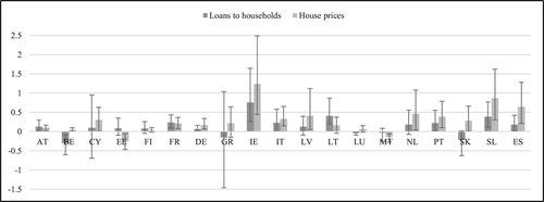
Figure A2. MCS-BGVAR-SV country-level results: trade with the euro area.

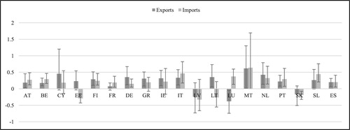
Figure A3. MCS-BGVAR-SV country-level results: trade with the extra-euro area.

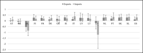
Figure A4. MCS-BGVAR-SV country-level results: trade prices with the euro area.

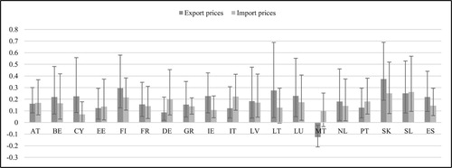
Figure A5. MCS-BGVAR-SV country-level results: trade prices with the extra-euro area.

A5. Robustness check V: modelling the euro area as EA-12 versus EA-19

Figure A6. MCS-BGVAR-SV country-level results: output.

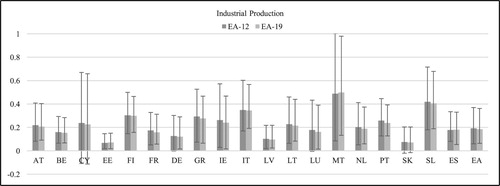
Figure A7. MCS-BGVAR-SV country-level results: sovereign yields.

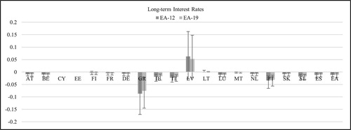
Figure A8. MCS-BGVAR-SV country-level results: inflation.

References

- Almansour, A., Aslam, A., Bluedorn, J., & Duttagupta, R. (2015). How vulnerable are emerging markets to external shocks? Journal of Policy Modeling, 37(3), 460–483. https://doi.org/10.1016/j.jpolmod.2015.03.009
- Altavilla, C., Carboni, G., & Motto, R. (2015). Asset purchase programmes and financial markets: Lessons from the Euro area. ECB Working Paper, No. 1864, November 2015, 52 p.
- Arias, J. E., Rubio-Ramirez, J. F., & Waggoner, D. (2014). Inference based on SVARs identified with sign and zero restrictions: Theory and applications. CEPR Discussion Paper, No. 9796, 70 p.
- Beck, R., Duca, I. A., & Stracca, L. (2019). Medium term treatment and side effects of quantitative easing: International evidence. ECB Working Paper, No. 2229, January 2019, 47 p.
- Benecká, S., Fadejeva, L., & Feldkircher, M. (2018). Spillovers from Euro area monetary policy: A focus on emerging Europe. Latvijas Banka Working Paper, No. 4/2018, 30 p.
- Bernanke, B. S., Reinhart, V. R., & Sack, B. P. (2004). Monetary policy alternatives at the zero bound: An empirical assessment. Board of Governors of Federal Reserve Systems (US), Finance and Economics Discussion Series, No. 2004–48, 100 p.
- Blattner, T. S., & Joyce, M. A. S. (2016). Net debt supply shocks in the Euro area and the implications for QE. ECB Working Paper, No. 1957, September 2016, 42 p.
- Bluwstein, K., & Canova, F. (2015). Beggar-thy-neighbor? The international effects of ECB unconventional monetary policy measures. CEPR Discussion Paper, No. 10856, 38 p.
- Boeckx, J., Dossche, M., & Peersman, G. (2017). Effectiveness and transmission of the ECB's balance sheet policies. International Journal of Central Banking, 13(1), 297–333.
- Bridges, J., & Thomas, R. (2012). The impact of QE on the UK economy – some supportive monetarist arithmetic. Bank of England Working Paper, No. 442, January 2012, 51 p.
- Burriel, P., & Galesi, A. (2018). Uncovering the heterogeneous effects of ECB unconventional monetary policies across euro area countries. European Economic Review, 101(C), 210–229. https://doi.org/10.1016/j.euroecorev.2017.10.007
- Chudik, A., & Fratzscher, M. (2012). Liquidity, risk and the global transmission of the 2007–08 financial crisis and the 2010–11 sovereign debt crisis. ECB Working Paper, No. 1416, February 2012, 46 p.
- Chudik, A., & Pesaran, M. H. (2013). Econometric analysis of high dimensional VARs featuring a dominant unit. Econometric Reviews, 32(5–6), 592–649. https://doi.org/10.1080/07474938.2012.740374
- Crespo Cuaresma, J., Feldkircher, M., & Huber, F. (2016). Forecasting with global vector autoregressive models: A Bayesian approach. Journal of Applied Econometrics, 31(7), 1371–1391. https://doi.org/10.1002/jae.2504
- Cushman, D., & Zha, T. (1997). Identifying monetary policy in a small Open economy under flexible exchange rates. Journal of Monetary Economics, 39(3), 433–448. https://doi.org/10.1016/S0304-3932(97)00029-9
- De Santis, R. A. (2016). Impact of the asset purchase programme on Euro area government bond yields using market news. ECB Working Paper, No. 1939, July 2016, 22 p.
- Dieppe, A., Legrand, R., & Van Roye, B. (2016). The BEAR Toolbox. ECB Working Paper, No. 1934, July 2016, 290 p.
- Eickmeier, S., & Ng, T. (2015). How do US credit supply shocks propagate internationally? A GVAR approach. European Economic Review, 74(C), 128–145. https://doi.org/10.1016/j.euroecorev.2014.11.011
- Feldkircher, M., Gruber, T., & Huber, F. (2020). International effects of a compression of euro area yield curves. Journal of Banking & Finance, 113(C). https://doi.org/10.1016/j.jbankfin.2019.03.017
- Feldkircher, M., & Huber, F. (2016). The international transmission of US shocks – evidence from Bayesian global vector autoregressions. European Economic Review, 81(C), 167–188. https://doi.org/10.1016/j.euroecorev.2015.01.009
- Fry, R., & Pagan, A. (2011). Sign restrictions in structural vector autoregressions: A critical review. Journal of Economic Literature, 49(4), 938–960. https://doi.org/10.1257/jel.49.4.938
- Gambacorta, L., Hofmann, B., & Peersman, G. (2014). The effectiveness of unconventional monetary policy at the zero lower bound: A cross-country analysis. Journal of Money, Credit and Banking, 46(4), 615–642. https://doi.org/10.1111/jmcb.12119
- Gambetti, L., & Musso, A. (2017). The macroeconomic impact of the ECB's expanded asset purchase programme (APP). ECB Working Paper, No. 2075, June 2017, 41 p.
- Garcia Pascual, A. I., & Wieladek, T. (2016). The European Central Bank's QE: A new hope. CEPR Discussion Paper, No. DP11309, 34 p.
- George, E. I., Sun, D., & Ni, S. (2008). Bayesian stochastic search for VAR model restrictions. Journal of Econometrics, 142(1), 553–580. https://doi.org/10.1016/j.jeconom.2007.08.017
- Georgiadis, G. (2015). Examining asymmetries in the transmission of monetary policy in the euro area: Evidence from a mixed cross-section global VAR model. European Economic Review, 75(C), 195–215. https://doi.org/10.1016/j.euroecorev.2014.12.007
- Georgiadis, G. (2017). To Bi, or not to Bi? Differences between spillover estimates from bilateral and multilateral multi-country models. Journal of International Economics, 107(C), 1–18. https://doi.org/10.1016/j.jinteco.2017.03.010
- Hartmann, P., & Smets, F. (2018). The first twenty years of the European Central Bank: Monetary policy. ECB Working Paper, No. 2219, December 2018, 96 p.
- Jarociński, M., & Karadi, P. (2020). Deconstructing monetary policy surprises – the role of information shocks. American Economic Journal: Macroeconomics, 12(2), 1–43. https://doi.org/10.1257/mac.20180090
- Karlsson, S. (2012). Forecasting with Bayesian vector autoregressions. Örebro university school of business, Working Paper, No. 12/2012, 101 p.
- Kastner, G., & Frühwirth-Schnatter, S. (2014). Ancillarity-sufficiency interweaving strategy (ASIS) for boosting MCMC estimation of stochastic volatility models. Computational Statistics & Data Analysis, 76(C), 408–423. https://doi.org/10.1016/j.csda.2013.01.002
- Koijen, R. S. J., Koulischer, F., Nguyen, B., & Yogo, M. (2016). Quantitative Easing in the Euro area: The dynamics of risk exposures and the impact on asset prices. Banque de France Document de Travail, No. 601, September 2016, 48 p.
- Moder, I. (2017). Spillovers from the ECB's non-standard monetary policy measures on South-Eastern Europe. ECB Working Paper, No. 2095, August 2017, 39 p.
- Pesaran, M. H., Schuermann, T., & Weiner, S. M. (2004). Modeling regional interdependencies using a global error-correcting macroeconometric model. Journal of Business & Economic Statistics, 22(2), 129–162. https://doi.org/10.1198/073500104000000019
- Stone, M., Fujita, K., & Ishi, K. (2011). Should unconventional balance sheet policies be added to the central bank toolkit? A review of the experience so far. IMF Working Paper, No. WP/11/145, 70 p.
- Vayanos, D., & Vila, J.-L. (2009). A preferred-habitat model of the term structure of interest rates. CEPR Discussion Paper, No. DP7547, November 2009, 61 p.