Measuring the effects of inflation and inflation uncertainty on output growth in the central and eastern European countries

ABSTRACT

This paper investigates how inflation and its uncertainty impact GDP growth in eight Central and Eastern European Countries. Inflation uncertainty series are created examining several GARCH models in combination with three different distribution functions, while the nonlinear effect of inflation and its uncertainty on GDP growth is assessed in the Bayesian quantile regression framework. We find that inflation has significantly smaller negative effect on GDP growth than inflation uncertainty, which confirms the Friedman hypothesis. This means that inflation in the selected countries has an indirect impact on GDP growth via inflation uncertainty. We find that countries with smaller economy, such as Latvia and Estonia experience more adverse effect from inflation uncertainty in both upturn and downturn conditions, probably because they are vulnerable to external inflationary shocks. As for the countries with bigger economy, inflation uncertainty shocks diminish GDP growth only in conditions when output growth is very low or negative.

KEYWORDS:

• Inflation
• inflation uncertainty
• GDP growth
• GARCH
• Bayesian quantile regression

JEL CODES:

• C11
• C21
• E23
• E31

1. Introduction

Nobel prize winner Friedman (1977) asserted that high and volatile inflation inhibits economic growth, and since then, a research about the effect of inflation on output growth became a relevant topic in macroeconomics. Fischer (1993) contended that growth is mainly affected through uncertainty, whereas the latter is generated through inflation, instability of the budget or current account. According to Friedman’s (1977) theory, high and unstable inflation causes an increase in inflation uncertainty that distorts the information content of prices, which consequently spills over to the efficient allocation of resources. Some papers, such as Lyziak (2016) and Caglayan et al. (2016), argued that in high inflation conditions, companies cannot detect profitable investment opportunities, because it impedes them to extract information about the relative prices of goods. In addition, during high-inflation times, external funds become prohibitively expensive due to increased information asymmetries. Both above-mentioned factors force companies to quit or postpone their fixed investment projects, which inevitably lowers output growth. Apergis (2005) listed more conduits through which inflation has an impact on economic growth. For instance, inflation can adversely affect savings, the structure of the tax system that transmits indirectly on investments, the activity of financial markets, the volatility in interest and exchange rates and the effect on the distribution of human capital. According to Grier and Grier (2006), there is little theoretical consensus on how inflation affects economic performance, since many papers found neutral, negative or even positive effect of average inflation on economic performance. The same situation is with inflation uncertainty, i.e. the influence of uncertainty on growth can either be positive or negative. Therefore, a new research on this topic could help in better understanding what is the impact of these two macro phenomena on output growth, and new conclusions might be of great benefit for the international community.

This paper tries to add to the literature by investigating how two macro fundamentals, inflation and inflation uncertainty, affect GDP growth in eight Central and Eastern European Countries (CEECs), which became the members of EU in 2004 – the Czech Republic, Poland, Hungary, Slovakia, Lithuania, Latvia, Estonia and Slovenia. In the analysis, we observe quarterly GDP data rather than monthly industrial production data, because GDP is wider economic aggregate, and as such, it describes economic activity more realistically. In other words, industrial production represents only a portion of the output, while GDP measures the total output. To be more specific, we put an effort to determine whether the price levels affect output directly via inflation, or indirectly via inflation uncertainty, or both. Inflation uncertainty can be viewed as the variance of unpredictable component of inflation, according to Grier and Perry (1998). The same authors also emphasized that uncertainty should be observed differently from variability, because uncertainty can be regarded as unpredictable fluctuations, whereas variability captures both unpredictable and predictable fluctuations. An important implication of this difference is that predictable components, which are included in a measure of variability, are not associated with any economic uncertainty. Grier and Perry (1998) asserted that variability, such as a moving standard deviation of the inflation, is not an appropriate measure to capture uncertainty.

We select these countries, because they conducted numerous and profound structural reforms in 90s with aim to become successful market economies, while at the same time they commenced the convergence towards the European Monetary Union (EMU), which presented an additional argument for price stability achievement (see, e.g. Berensmann and BeyfuB, 2002; Živkov et al., 2014; Njegić et al., 2017; Svilokos et al., 2019; Alper, 2020). As a result, these countries realized relatively high annual GDP growth rates in past two decades (see Table 1), and finding out whether and how inflation and its uncertainty influence output growth is one of the important questions for monetary authorities for the countries which conduct independent monetary policy (the Czech Republic, Poland and Hungary). On the other hand, this question is also important for the countries which joined EMU (Slovakia, Baltic states and Slovenia), i.e. the results can be useful for their companies, because they can use this knowledge to design their business strategies accordingly. It should be said that this topic is particularly important for countries which pursue independent monetary policy, because increased inflation uncertainty can be caused by the public’s lack of confidence in the policy-maker’s attitude towards stabilizing prices with monetary policies (see Ball, 1992). According to Hayford (2000), private agents are generally uncertain how to perceive monetary authorities, because they can be recognized as either conservatives or liberals. The former only care about how to keep inflation low, while liberals are willing to trade higher inflation for higher economic growth. In low inflation conditions, both types of monetary authorities will act in direction to keep inflation low. However, in higher inflation circumstances, conservatives will immediately disinflate, while liberals may waver. Therefore, it is important to give a hint to which type of policy-makers, particular monetary authorities of the Czech Republic, Poland and Hungary belong to.

Table 1. Average GDP growth rates and nominal GDP of the selected CEECs.

	CZE	POL	HUN	SLK	LIT	LAT	EST	SLO
GDP growth rates^a	2.65	3.88	2.60	3.70	4.06	3.99	3.86	2.59
Nominal GDP in millions of US$^b	246,953	565,854	170,407	106,552	53,641	35,045	31,038	54,154

^a Source: OECD statistics in the period 1998–2019.

^b Source: International monetary fund in 2019.

Besides, specific necessity for this type of research arises from the fact that serious lack of relevant studies on this subject is present in the international literature, while this contention particularly applies for CEECs. As a matter of fact, we know only for two papers that did this type of research on CEECs (see Hasanov and Omay, 2011; Pintilescu et al., 2014). It can be seen in Table 1 that all CEECs had relatively high GDP growth rates in the observed period, and that especially applies for Poland, Slovakia and three Baltic states.

In our research, we follow the paper of Chang and He (2010) and measure the influence of both phenomena on GDP growth jointly, because inflation and its uncertainty are closely associated, which means that exclusion either one of the variables will produce a biased estimate of the coefficient of the included variable. In addition, we want to put an emphasis on the accurateness of the results. In that manner, we endeavour to measure inflation uncertainty as precise as possible, because Caglayan et al. (2016) asserted that the impact of inflation uncertainty on output growth depends on the approach that one uses to construct measures of uncertainty. Recent paper of Živkov et al. (2019) constructed optimal inflation uncertainty time-series by using several types of GARCH model along with three traditional and three innovative distribution functions. Referring to this paper, we also consider different GARCH models in combination with three different distributions. In particular, for every inflation time-series, we estimate two traditional GARCH models – simple GARCH and GJR-GARCH model of Glosten et al. (1993) as well as nonlinear asymmetric GARCH (NA-GARCH) model of Engle and Ng (1993). All these models are combined with normal, Student-t and normal inverse Gaussian distribution of Barndorff-Nielsen (1997).

Besides, according to Chowdhury et al. (2018), the majority of empirical studies assume that the underlying relationships between inflation phenomena and output are constant over the entire sample period, which implies that the causal links are stable over time. However, these authors strongly asserted that this assumption does not hold in practice. Therefore, in order to avoid this potential estimation bias, we hypothesize that nonlinear nexus exists between inflation (inflation uncertainty) and output, and use very novel estimation tool that can gauge accurately and reliably the relationship between underlying variables. This methodology is the Bayesian quantile regression (BQR). In other words, after the construction of optimal conditional volatilities, we insert these variables and GDP growth time-series in the multivariate BQR framework. General characteristic of the quantile regression methodology is the fact that it can provide an insight about the transmission effect from inflation and its uncertainty towards output in different market conditions – downturn (lower quantiles), normality (intermediate quantiles), and economic prosperity (upper quantiles). More specifically, QR technique can recognize the underlying nonlinearities in the data, which prevents biased conclusions. The BQR approach is an upgrade, comparing to the traditional quantile regression of Koenker and Bassett (1978), because it uses Bayesian inference to calculate quantile parameters, that is, Markov Chain Monte Carlo (MCMC) algorithm in the estimation process. This procedure ensures an efficient and exact values of the quantile parameters, which means that all estimated Bayesian quantile parameters are highly statistically significant and unbiased if confidence intervals are narrow (see, e.g. Pal and Mitra, 2015). In particular, the BQR methodology decreases the length of credible intervals and increases the accurateness of quantile estimates in comparison with the traditional quantile regression OLS approach of Koenker and Bassett (1978).

To the best of our knowledge, this paper differentiates from the existing literature along several dimensions. First, this paper is the first one that investigates the impact of inflation (inflation uncertainty) to output in CEECs, using elaborate methodologies for the construction of conditional volatilities. Second, novelty is also a usage of sophisticated BQR technique that can determine a nonlinear nexus between the variables, providing, but at the same time also reliable results and trustworthy conclusions.

Besides introduction, the rest of the paper is structured as follows. Section 2 provides literature review. Section 3 explains used methodologies. Section 4 contains dataset and the way in which conditional volatilities are created. Section 5 presents the results, while Section 6 discusses the results. Section 7 estimates quantile parameters in two different subsamples – before and after joining the EU. The last section concludes.

2. Literature overview

Since the introduction of the Friedman’s hypothesis, a great number of empirical investigations have been conducted, but with heterogeneous results. This is the case because different methodologies were applied, different countries were examined and in different time periods. Some papers researched only the impact of inflation uncertainty on output, while others investigated the links between inflation, its uncertainty and economic activity. From the first group of papers, we can single out the study of Apergis (2005), who explored empirically the connection between inflation uncertainty and economic growth via panel data analysis that includes OECD economies in relatively long time period from 1969 to 1999. He concluded that inflation uncertainty has an adverse impact on GDP growth in the majority of the countries under investigation. Another study was conducted by Caglayan et al. (2016), who researched the impact of inflation uncertainty on output growth for the United States between 1960 and 2012. Their results indicated that inflation uncertainty exerts a negative and regime-dependent impact on output growth. Jiranyakul and Opiela (2011) researched the impact of inflation uncertainty on output growth in Thailand, using AR(p)-cccGARCH(1,1) model. They reported a positive relation from inflation to inflation uncertainty, whereas increased inflation uncertainty decreases output. The paper of Wu et al. (2003) examined the effects of inflation uncertainties on real GDP in the U.S.A. and claimed that different sources of inflation uncertainty have different impacts on real GDP. They found that uncertainty from changing regression coefficients has negative impacts on real GDP. On the other hand, the effect of uncertainty due to heteroscedasticity in disturbances on real GDP is insignificant, according to their results. Contrary to the previously listed papers, Fountas (2010) strongly excepted findings that inflation uncertainty is not detrimental to output growth. He investigated the relationship between inflation uncertainty, inflation and growth using a data sample on 22 industrial countries.

As for the papers that measured the nexus between inflation, inflation uncertainty and GDP, among others, it is worth to mention the paper of Wilson (2006). This author considered the Japanese case, applying a bivariate EGARCH-M model. He argued that increased inflation uncertainty is associated with higher average inflation and lower average growth. In addition, he found an evidence that increased growth uncertainty raises average inflation. Grier and Grier (2006) utilized an augmented multivariate GARCH-M system for the Mexican case. They concluded that average inflation lowers output growth in Mexico, but it happens via raising uncertainty about future inflation. Chang and He (2010) used a bivariate Markov switching model to investigate how inflation and inflation uncertainty affect output growth in the U.S.A., covering a long time period, from 1960Q1 to 2003Q3. They found that inflation cannot affect the output growth, while inflation uncertainty can have a non-linear negative effect on the output growth. They contended that impact from inflation uncertainty to output growth can be quite substantial, suggesting that inflation uncertainty is the major factor that influences the output growth. Huang et al. (2019) tried to find out whether the adoption of inflation targeting (IT) helps in reduction of output-inflation trade-off. They used annual panel data of 74 countries. Their results suggested that the adoption of inflation targeting is significantly associated with lower trade-off between output and inflation. In addition, they argued that the adoption of inflation targeting leads to a lower level of output-inflation trade-off in both developing and developed countries, while on average, the trade-off is larger in developing countries.

3. Research methodologies

3.1. Estimation of conditional volatilities

Our goal is to find an optimal proxy for inflation uncertainty, and in that process, we consider three GARCH class models – simple GARCH, GJR-GARCH and NA-GARCH, along with three distribution functions – normal, Student-t and normal inverse Gaussian (NIG) distribution.¹ We employ GARCH models in the construction of inflation uncertainty because this model ensures that the uncertainty, associated with inflation, originates primarily from the unpredictable component of inflation, which is in line with the neoclassical thesis, according to Apergis (2005).

In this elaborate and time-consuming procedure, we estimate nine different GARCH models for every inflation, seeking the lowest information criterion (AIC, BIC or HQ) that indicates which model is the optimal one. Consequently, the best fitting GARCH model is used to create conditional volatility of inflation, which represents inflation uncertainty. For every model, we consider $AR\left(n\right)$ specification in the mean equation, where $n$ stands for a lag order. This is done in order to circumvent spurious regression that can be caused by a serial correlation. The error term $\left({ϵ}_t\right)$ in the mean equation follows the ${ϵ}_t\sim i.i.d.\left(0,h_t\right)$ process. Equations (1)–(3) define mathematical specifications of three different GARCH models – simple GARCH, GJR-GARCH and NA-GARCH, respectively. (1) ${\sigma }_t^2=c+\alpha {ϵ}_{t-1}^2+\text{β}{\sigma }_{t-1}^2$(1) (2) ${\sigma }_t^2=c+\alpha {ϵ}_{t-1}^2+\text{β}{\sigma }_{t-1}^2+\gamma {ϵ}_{t-1}^2{I}_{t-1};I_{t-1}=\left\{\begin{array}{cc}1& \text{if}{ϵ}_{t-1}<0\\ 0& \text{if}{ϵ}_{t-1}>0\end{array}\right.$(2) (3) ${\sigma }_t^2=c+\text{β}{\sigma }_{t-1}^2+\alpha {\sigma }_{t-1}^2({ϵ}_{t-1}^2-\gamma {)}^2$(3) where ${\sigma }_t^2$ is a conditional variance in period t. $c$ is a constant term, β term captures the persistence of volatility, $\alpha$ gauges an ARCH effect, while $\gamma$ is the coefficient that measures asymmetric response of volatility to positive and negative shocks. For every GARCH specification, we consider two traditional distributions – normal $ϵ\sim N\left(0,h_t\right)$, Student-t $ϵ\sim St\left(0,h_t,\nu \right)$ and one unconventional heavy tailed distribution – normal inverse Gaussian distribution $ϵ\sim NIG\left(0,h_t,\nu ,\kappa \right)$ of Barndorff-Nielsen (1997). Unconventional NIG distribution is chosen, because it can recognize heavier tails than the normal distribution that are often skewed and asymmetric. These characteristics can contribute to more precise measurement of conditional volatilities. In order to be parsimonious as much as possible, we present in Equation (4), mathematical formulation only for the normal inverse Gaussian (NIG) distribution. (4) $\left(x\right)=\frac{\delta \alpha \text{exp}\left(\delta \sqrt{{\alpha }^2-{\text{β}}^2}\right)K_1\left(\alpha \sqrt{{\delta }^2+{\left(x-\mu \right)}^2}\right)\text{exp}\left(\text{β}\left(x-\mu \right)\right)}{\pi \sqrt{{\delta }^2+{\left(x-\mu \right)}^2}};x\to \pm \mathrm{\infty }$(4) where $\delta >0$ and $0<\left|\text{β}\right|\le \alpha$. Scale and location are determined by the $\mu$ and $\delta$ parameters, respectively. Shape and density are controlled by $\alpha$ and $\text{β}$ parameters, respectively. $K_1$ is modified Bessel function of the third kind. Symmetric distribution happens if $\text{β}=0$.

The reason why we choose to estimate two asymmetric GARCH models beside ordinary GARCH model comes from the paper of Buth et al. (2015). This author claimed that the Friedman–Ball argument assumes that new information about low inflation should reduce, rather than increase, inflation uncertainty. Therefore, the simple GARCH specification with a symmetric effect might not be consistent with the notion of the Friedman–Ball argument.

3.2. Bayesian quantile regressions

After the creation of inflation conditional volatilities, we can gauge how inflation and its uncertainty affect GDP growth in the selected CEECs. For this purpose, we use the quantile regression technique, estimated with MCMC approach. Generally speaking, QR methodology extends the mean regression model to conditional quantiles of the response variable. In other words, this approach gives a more complex and informative view of the relations between the dependent variable and the covariates, because it estimates how a set of covariates affect the different parts of the regressand distribution. QR methodology has been widely used by many researchers from various theoretical disciplines (see, e.g. Maestri, 2013; Vilerts, 2018; Živkov et al., in press).

We start the explanation of the Bayesian QR methodology by implementing the standard linear model as in Equation (5): (5) $y_{t,i}={\omega }_1+{\omega }_2{y}_{t-1,i}+{\omega }_3{\pi }_{t,i}+{\omega }_4{\sigma }_{t,i}^2+{ϵ}_i$(5) where $y_{t,i}$ is the quarterly GDP growth rate of particular country $i$, ${\pi }_{t,i}$ is the inflation rate, while ${\sigma }_{t,i}^2$ is the conditional volatility of inflation, obtained from the optimal GARCH model, which represents inflation uncertainty measure. ${\omega }_1$ parameter is constant, ${\omega }_2$ stands before autoregressive term of GDP growth, and it measures the persistence of output growth, while ${\omega }_3$ and ${\omega }_4$ parameters gauge the transmission effect of inflation and its uncertainty to GDP growth, respectively.

Benoit and van den Poel (2017) contended that in BQR framework, the regression coefficient in the case of all quantiles can be found by solving Equation (6): (6) $\widehat{\text{β}}\left(\tau \right)=\text{argmin}\sum _{i=1}^n{\rho }_{\tau }(y_i-{x^{\mathrm{\prime }}}_i\text{β});\text{β}\in \mathrm{\Re }$(6) where $\tau \in \left(0,1\right)$ is any quantile of interest, while ${\rho }_{\tau }\left(z\right)=z\left(\tau -I\left(z<0\right)\right)$ and $I(\cdot )$ stands for the indicator function. The quantile $\widehat{\text{β}}\left(\tau \right)$ is called the ${\tau }^{\mathrm{t}\mathrm{h}}$regression quantile. When $\tau =0.5$, it corresponds to median regression. In the Bayesian procedure, QR parameters are estimated with the usage of the Markov Chain Monte Carlo (MCMC) algorithm. We decide to use this particular estimation methodology, because it is efficient procedure in the low data environment, such as ours. More specifically, it produces exact estimates of the quantile parameters $\widehat{\text{β}}\left(\tau \right)$, which can measure accurately and reliably the nonlinear transmission effects from inflation and its uncertainty to GDP growth. In other words, if confidence intervals are relatively narrow, all estimated Bayesian quantile parameters can be regarded as statistically significant.

In addition, we have to mention a potential problem that can arise due to the fact that inflation uncertainty is a generated regressor in Equation (5). In particular, we refer to a caveat of Pagan (1984), in order to ensure the correctness of our approach. According to this author, three issues can emerge from this situation: (1) consistency of estimation, (2) efficiency of estimation and (3) valid inference. Pagan (1984) contended that when only unlagged predictions appear as regressors, which is the case in Equation (5), the two-step regression estimator satisfies three aforementioned conditions. Therefore, we can be sure that our approach does not generate biased estimates.

4. Dataset and creation of inflation uncertainty proxy

This paper uses quarterly time-series of GDP growth and inflation rate of eight Central and Eastern European Countries – the Czech Republic, Poland, Hungary, Slovakia, Lithuania, Latvia, Estonia and Slovenia. All GDP growth and inflation time-series are seasonally adjusted, using filter-based methods of seasonal adjustment, known as X11 style method. The sample ranges from January 1998 to December 2019, and all time-series are collected from OECD statistics website. Table 2 contains descriptive statistics for quarterly GDP growth and inflation rate time-series, including first four moments and Jarque–Bera test for normality. Before Bayesian QR computation, we need to create inflation uncertainty time-series, and for that reason we additionally calculate Ljung–Box Q-statistics for level and squared residuals of inflation rates in Panel B of Table 2. As can be seen, all empirical inflation rates report the presence of autocorrelation and heteroscedasticity, which means that some form of ARMA-GARCH model might be appropriate. Besides, according to Table 2, all time-series have pronounced skewness and kurtosis, which means that unconventional NIG distribution function might successfully capture these non-normal empirical features.

Table 2. Descriptive statistics of quarterly GDP growth and inflation.

	CZE	POL	HUN	SLK	LIT	LAT	EST	SLO
Panel A. GDP growth
Mean	0.670	0.961	0.671	0.902	0.954	0.930	0.902	0.632
Standard deviation	0.812	0.913	0.910	1.665	1.844	2.122	1.900	1.170
Skewness	−1.470	0.405	−2.254	−1.710	−4.147	−0.496	−3.490	−1.165
Kurtosis	8.907	4.116	10.311	17.935	30.694	3.805	22.941	7.022
JB test	157.8 (0.000)	6.9 (0.032)	267.4 (0.000)	851.0 (0.000)	3029.6 (0.000)	5.9 (0.052)	1618.1 (0.000)	78.3 (0.000)
Panel B. Inflation rate
Mean	2.629	3.192	5.013	3.977	2.481	3.662	3.573	3.432
Standard deviation	2.4	3.2	3.6	3.6	2.8	3.9	2.9	2.9
Skewness	2.243	1.373	0.804	1.240	1.323	1.529	0.695	0.641
Kurtosis	9.544	4.831	3.805	4.687	5.223	5.972	3.909	2.187
JB test	230.8 (0.000)	39.9 (0.000)	11.9 (0.003)	33.0 (0.000)	43.8 (0.000)	66.7 (0.000)	10.1 (0.006)	8.5 (0.015)
LB(Q)_20	0.000	0.000	0.000	0.000	0.000	0.000	0.000	0.000
LB(Q^2)_20	0.000	0.000	0.000	0.000	0.000	0.000	0.000	0.000

Notes: JB stands for coefficients of Jarque–Bera normality test. p-values are in parentheses for JB test. LB(Q) and LB(Q²) tests denote p-values of Ljung–Box Q-statistics of level and squared residuals for 20 lags.

In the process of GARCH estimation, we find that $AR\left(1\right)$ order in the mean equation successfully resolve the problem of autocorrelation in the Czech and Polish cases, whereas $AR\left(2\right)$ order is enough for all other countries. We present the results of Li–Mak tests in Table 3 that are performed on the GARCH residuals, and they all confirm the absence of autocorrelation and heteroscedasticity. Li and Mak (1994) test statistics is computed because this measure is more robust when residuals from GARCH model are in question.

Table 3. Results of Li–Mak² tests for autocorrelation and heteroscedasticity.

	CZE	POL	HUN	SLK	LIT	LAT	EST	SLO
Li–Mak test (Q)	4.040 (0.094)	1.261 (0.261)	0.311 (0.577)	1.766 (0.184)	0.522 (0.470)	2.235 (0.135)	0.026 (0.872)	2.763 (0.096)
Li–Mak test (Q^2)	0.870 (0.351)	0.746 (0.388)	1.415 (0.234)	2.712 (0.113)	2.954 (0.107)	3.025 (0.091)	3.001 (0.106)	0.679 (0.410)

Notes: Values in parentheses are probabilities.

Therefore, an appropriate lag order in the mean equation is applied for every country, while an inflation uncertainty time series is created via optimal GARCH model in combination with the best fitting distribution function. Table 4 contains the results of three information criteria – AIC, BIC and HQ. We estimate three different information criteria for robustness purposes, and greyed values signal the lowest value. As can be seen, only in three out of eight cases (CZE, HUN and LIT) all three criteria point to the same GARCH model, whereas in all other cases AIC and HQ differentiate in regard to BIC. When information criteria have no unison decision, we give an advantage to the model that is preferred by AIC and HQ. In particular, AIC is preferred because it is the usual approach (see, e.g. Živkov et al., 2019, and Usman et al., 2019). In addition, AIC and HQ are consistent in indicating the best model. It is clear that a common pattern can be found in Table 4, in a sense that GJRGARCH and NAGARCH models outperform ordinary GARCH model, which means that asymmetry of responses is important. However, it can also be noticed that GJRGARCH and NAGARCH models dominantly outperform simple GARCH only according to AIC and HQ, but not BIC. The reason could lie in the fact that SIC generally favours more parsimonious models, i.e. with lower number of parameters. In addition, in 6 out of 8 cases, the best model is GJRGARCH, according to AIC and HQ. This indicates that simpler GJRGARCH model, in relation to NAGARCH model, better recognizes asymmetric effect, probably because we use relatively short quarterly time-series. Based on the results in Table 4, we can assert that for each country a particular GARCH model with specific distribution function is optimal, which gives us a confidence that our approach of combining GARCH models with different distributions is justifiable.

Table 4. Estimated three information criteria for the selected GARCH models of inflation.

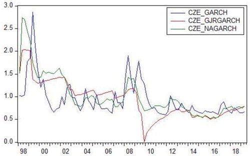
Applying different GARCH specification, we determine that created inflation uncertainties follow similar trend, but they differ between themselves noticeably. In order to illustrate this assertion, we present in Figure 1 estimated inflation uncertainty time-series for the Czech Republic, derived from the three different GARCH models with optimal distribution for each model. Since inflation uncertainties have visible distinctions, this gives us a justification to test different GARCH models for every country and find the optimal one. This is important, because suboptimal inflation uncertainty time-series would probably have an impact on subsequent computation of quantile estimates that can lead us to erroneous conclusions.

Figure 1. Three inflation uncertainty time-series estimated with three different GARCH models.

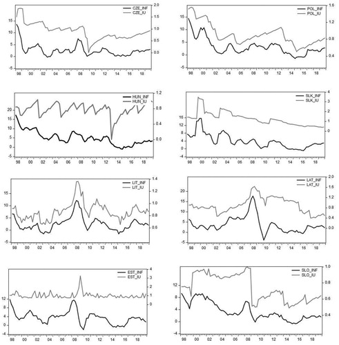
Therefore, based on the results in Table 4, we create conditional volatilities with the best fitting GARCH model. Figure 2 presents graphical illustration of both inflation and inflation uncertainty time-series for every country involved.

Figure 2. Quarterly presentation of inflation and inflation uncertainty time series.

Notes: Black (grey) line denotes dynamics of inflation (inflation uncertainty). Abbreviation INF stands for inflation, whereas IU is a mark for inflation uncertainty.

Before presentation of the estimated Bayesian QR parameters, we need to check for their validity, and this can be done by a visual inspection of the convergence of the MCMC chains. So-called trace plots show the evolution of the MCMC draws over the iterations, and they are presented in Figure 3. We use 1000 iterations for our computations, which is a way longer than the length of the empirical time-series (88 quarterly observation). In addition, we use 200 burn-in observations. The longer MCMC chain is, the more reliable quantile estimates are. MCMC chain convergence implies the absence of (large) bias of the estimated parameters. This gives us a confidence that estimated Bayesian quantile parameters are relatively trustworthy.

Figure 3. Trace plots for median quantile of GDP(-1), inflation and inflation uncertainty for the Czech Republic.

Note: GDP(-1) indicates first-order autoregressive term of GDP growth, INF stands for inflation, while IU denotes inflation uncertainty.

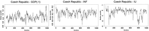
Due to the fact that trace-plots of all countries are very similar, which also applies for all quantiles, we present only median quantiles trace plots in Figure 3 for the Czech Republic. In particular, Figure 3 portrays the trace plots of the MCMC chain of the median quantiles, $\widehat{\text{β}}\left(\tau \right)=0.5$, of the selected macroeconomic time-series for the Czech Republic. As can be seen, all trace-plots have very good dynamics, in a sense that the MCMC sampler quickly moves to the stationary distribution. All other trace plots can be obtained by request. It should be said that MCMC chain convergence does not imply anything about statistical significance of the estimated parameters, but the statistical significance of the parameters can be rather assessed by Bayesian credible intervals, which are presented in Figure 4 in the next section.

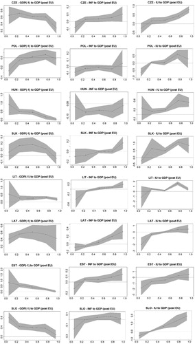
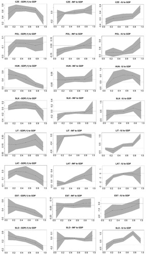
Figure 4. Graphical illustration of the estimated Bayesian quantile parameters.

Note: Left-hand column contains the plots that show the persistence of the GDP growth. Middle column shows the effect of inflation on GDP growth, while right-hand column depicts the effect of inflation uncertainty on GDP growth. Shaded areas represent Bayesian confidence intervals at 70% probability level.

5. Empirical results

This section endeavours to answer the question how (whether) inflation and its uncertainty affect GDP growth in the selected CEECs. The quantile estimates reveal the size of the effect that transmits from inflation and its uncertainty towards GDP growth in different market conditions – downturn, normality and upturn. In the following, we comment estimated Bayesian quantile parameters in Table 5, while Figure 4 presents graphical illustrations of these parameters with 70% probability confidence intervals.

Table 5. Estimated Bayesian quantile parameters for the selected CEECs.

	Estimated quantiles with MCMC
	0.05	0.25	0.5	0.75	0.95	0.05	0.25	0.5	0.75	0.95
	Czech Republic					Poland
${\omega }_1$	−0.328	−0.019	0.173	0.376	1.058	−0.097	0.486	1.018	1.302	2.014
${\omega }_2$	0.496	0.692	0.679	0.622	0.311	−0.204	−0.017	−0.024	−0.079	−0.042
${\omega }_3$	−0.070	−0.017	0.002	0.029	0.054	−0.094	−0.042	−0.036	0.007	0.022
${\omega }_4$	−0.261	−0.024	0.026	0.107	0.497	−0.015	−0.022	0.072	0.235	0.732
	Hungary					Slovakia
${\omega }_1$	−0.962	−0.134	0.231	0.702	1.631	−0.308	0.194	0.508	0.651	2.362
${\omega }_2$	0.691	0.645	0.425	0.173	0.056	0.044	0.119	0.126	0.076	−0.254
${\omega }_3$	0.012	−0.001	0.002	0.004	0.027	−0.228	−0.074	−0.055	−0.047	0.131
${\omega }_4$	−0.410	−0.092	0.266	0.408	0.089	0.013	0.296	0.400	0.753	0.552
	Lithuania					Latvia
${\omega }_1$	−0.565	0.948	0.713	1.165	1.807	−0.217	0.265	0.500	1.444	4.151
${\omega }_2$	0.191	0.160	0.191	0.249	0.123	0.209	0.316	0.285	0.169	0.028
${\omega }_3$	−0.400	−0.020	−0.007	0.033	−0.042	−0.086	−0.082	0.075	0.204	0.245
${\omega }_4$	−0.200	−0.718	0.214	0.421	1.257	−2.276	−0.581	−0.110	−0.266	−0.983
	Estonia					Slovenia
${\omega }_1$	0.200	0.987	1.801	1.978	2.898	−1.626	−0.282	0.132	0.101	1.895
${\omega }_2$	0.570	0.526	0.406	0.264	0.080	0.469	0.369	0.269	0.119	−0.107
${\omega }_3$	−0.103	−0.005	−0.009	0.029	0.035	−0.048	0.003	−0.003	−0.036	0.039
${\omega }_4$	−1.679	−1.124	−1.136	−0.500	−0.034	−0.191	0.266	0.555	1.537	0.557

However, before we address our findings, it should be noted that in some quantile plots in Figure 4, lower and upper confidence intervals of the tail quantiles are relatively wide, which means that the interpretation of these results should be performed with caution. The reason why confidence intervals are broader for some tail quantiles probably lies in the fact that 0.05th and 0.95th quantiles depict extreme situations, that is, when GDP is very small (or negative) or very high, and these situations are very rare taking into account our low-data sample. Due to very small number of observations in the tails of the empirical distribution, Bayesian QR needs to broaden confidence intervals in order to preserve reliability of the Bayesian QR parameters.

According to Table 5, it is interesting to note that an asymmetric effect is well documented, which means that significant difference exists between left and right tail quantiles, and this testifies about the nonlinear nexus between the underlying fundamentals. ${\omega }_3\mathrm{a}\mathrm{n}\mathrm{d}{\omega }_4$ parameters show the size of the spillover effect across the quantiles from inflation and inflation uncertainty towards GDP growth, whereas ${\omega }_2$ parameter gauges the persistence of output growth. According to the results in Table 5 and Figure 4, the effect of lagged GDP growth to current GDP growth, in most cases, deteriorates gradually when higher quantiles are observed in respect to lower quantiles. This means that GDP growth can achieve steady growth rates and continuity more easily when GDP growth is relatively low, which is portrayed by lower quantiles. These results are highly expected, and this scenario applies for all countries, except Poland. For Poland, we report that GDP persistence do not exist, that is, steady continuity of GDP growth, quarter to quarter, is not found, although Poland has relatively high average growth rate (see Table 1). The reason for such results probably lies in the fact that Poland is the largest and most diversified economy among the selected countries. This means that different business cycles probably exist between different sectors of the economy. In other words, when some external shock or recession hits Polish economy, different sectors endure consequences in different magnitude. The same applies for the periods of market prosperity. Speaking differently, well-diversified economy experiences the effects of shocks at different rates in different sectors, and this could be the reason why GDP persistence is not found in Poland. In the cases of all other countries, particularly small economy countries, we find a unique pattern in a sense that GDP persistence diminishes under higher GDP growth rates (higher quantiles) and vice versa.

${\omega }_3$ and ${\omega }_4$ parameters explain how inflation and its uncertainty affect GDP growth across the quantiles. Several interesting findings can be highlighted. First of all, we find in five out of eight cases in 0.05th quantile that inflation has smaller negative effect on GDP growth than inflation unpredictability (inflation uncertainty) when GDP growth is negative or very low. These results stand in line with the Friedman hypothesis, who explained that increased inflation uncertainty rather than high inflation tends to adversely affect real economic activity, which consequently divert resources and reduce the allocative efficiency of the price system, causing lower ability of the economy to grow. In other words, no matter how inflation is high, economic subjects can adjust to its level and adapt their business activities as long as particular level of inflation is stable in relatively long time period. On the other hand, frequent changes of inflation level bring uncertainty in the public’s confidence about the policy-maker’s attitude towards stabilizing prices with monetary policies, according to Ball (1992), and then aforementioned negative effects of inflation uncertainty came to the fore. However, in interpretation of 0.05th quantile, we should be cautious because our sample covers global financial crisis, and during that time, both inflation uncertainty increased and GDP growth decreased substantially. This means that significant GDP downturn, which is recorded at 0.05th quantile, stems from the previous overheating and the global financial crisis, and not from the increase of inflation uncertainty. Therefore, at 0.05th quantile, we should talk about association between these two variables rather than an impact.

In addition, regarding the 0.05th quantile, the same cautious explanation should be applied on inflation. In other words, it can be seen that negative effect of inflation on GDP growth is relatively low in all countries (see Table 5), while the impact is stronger at lower quantiles, which represent low (or negative) GDP growth. However, in most countries, the negative effect of inflation to GDP is below 0.1. In particular, the strongest negative effect is detected in Lithuania and Slovakia, with the magnitude of −0.400 and −0.228, respectively at ${\tau }^{0.05}$ quantile. However, due to the fact that confidence intervals for Lithuania at 0.05th quantile are very wide, these results should be observed with great reserve. As for Slovakia, the confidence intervals are much narrower (see Figure 4), and thus, they are more reliable. Generally speaking, all ${\omega }_3$ parameters are relatively low, which coincides with general belief that inflation has relatively limited effect on GDP growth. For instance, our results concur very well with the findings of Grier and Grier (2006) and Chang and He (2010). The former study investigated the case of Mexico, using vector autoregression (VAR) type model, and the authors found little evidence of a direct negative nonlinear effect of average inflation on growth, which is very similar to our results. The latter paper researched the US case, employing a bivariate Markov regime switching model and they did not find a direct effect of inflation on output growth. Besides, very low effect of inflation on GDP growth is additionally strengthened by the fact that at higher GDP growth rates (higher quantiles), the negative effect of inflation gradually deteriorates.

Due to the fact that we do not find strong effect of inflation on GDP growth, while the impact of inflation uncertainty is sizable, it can be concluded that inflation in the selected CEECs has an indirect impact on GDP growth via inflation uncertainty, which is in line with the Friedman (1977) hypothesis. This assertion coincides very well with the previously mentioned paper of Grier and Grier (2006), who researched the Mexican case and contended that any significant negative effect of average inflation on output growth in Mexico operates indirectly through inflation uncertainty. Besides the study of Grier and Grier (2006), some other papers also reported significant negative spillover effect from inflation uncertainty towards GDP growth. For instance, Apergis (2005) researched 17 OECD countries in a panel and concluded that inflation uncertainty has an adverse impact on economic growth in the majority of the countries under investigation. Chang and He (2010) studied the US case and reported that inflation uncertainty has highly significant negative effect on GDP growth. Wilson (2006) documented that increased inflation uncertainty raises average inflation and lowers average growth in Japan.

However, looking at Table 5, it should be added that inflation uncertainty also has a positive effect on GDP growth, and we find that this effect is pretty conspicuous in some countries in conditions when GDP records strong growth rates (${\tau }^{0.95}$ quantile). At first sight, these results might seem puzzling, but Chowdhury et al. (2018) offered a viable explanation. He investigated the UK and US cases and contended that, during economic slowdown, cash flows to private sector are diminished, while the private firm’s balance sheets are weak. These conditions compel companies to delay or even cancel the investment projects, which reflect to output growth detrimentally. On the other hand, during the period of expansion, cash flows to the firms are relatively high, which is a favourable situation regardless of the changes in inflation uncertainty. Therefore, in these conditions, companies are willing to finance new investment projects, without worrying what inflation unpredictability might be. The readiness of companies to invest even when inflation uncertainty is present, raises output growth, and this is the reason why we find positive inflation uncertainty parameters, especially at higher quantiles. A reasoning of Dotsey and Sarte (2000) also can be mentioned, although explanation of these authors has weaker economic argumentation, comparing with the paper of Chowdhury et al. (2018). Dotsey and Sarte (2000) claimed that inflation uncertainty can raise GDP growth due to precautionary savings, which in turn induces higher GDP growth. According to Table 5, high and positive effect of inflation uncertainty to GDP growth is particularly visible in the cases of Slovenia, Lithuania, Slovakia and Poland. For these countries, estimated Bayesian quantile parameters at ${\tau }^{0.95}$ quantile are 0.557, 1.257, 0.552 and 0.732, respectively, which is relatively high. It should be noted that in some cases ${\tau }^{0.75}$ quantile parameters are also relatively high, which speaks in favour that inflation uncertainty does not have negative effect on GDP when the economy records high growth rates. On the other hand, only in cases of Latvia and Estonia, we find negative parameters across all the quantiles. Next section discusses the results and tries to find an economic logic behind the empirical findings.

6. Discussion of the results

This section tries to explain the results through the lens of some peculiarities that is characteristic for particular countries. Most of the discussion in this section is devoted to the effect of inflation uncertainty on GDP, because results indicate that inflation uncertainty has stronger impact on GDP than inflation.

First interesting finding is related to relatively small economies – Baltic states and Slovenia. In other words, for Latvia and Estonia it can be seen that the estimated Bayesian ${\omega }_4$ quantile parameters are negative in all quantiles, which is off the usual pattern, while for Lithuania and Slovenia, negative quantile estimates are detected in the first two quantiles and in the first quantile, respectively. This means that inflation uncertainty has negative effect on output growth in all economic conditions for the smallest economies – Latvia and Estonia, while for relatively larger economies, such as Lithuania and Slovenia, it applies for conditions of extreme and moderate downturn (${\tau }^{0.05}$ and ${\tau }^{0.25}$ quantiles). A possible explanation for these results could be as follows. Latvia and Estonia have relatively small economy (see Table 1), which means that they are not so diversified, and as such, they could be more exposed to external inflationary shocks. Besides, according to Table 2, average inflation in Latvia and Estonia is relatively low, thus it cannot be said that inflation uncertainty shocks come from within. In that regard, we should also mention the fact that Estonia and Latvia joined ERM2 in June 2004 and May 2005, respectively, while later on, they adopted euro. This means that these countries had stable currencies, which also contributed to their inflation stability. Therefore, a more probable explanation is that some other (external) factors have some influence on the inflation in these two Baltic states, whereas a sizable portion of this influence most likely goes to commodity price shocks, such as energy and food (see Kamber and Wong, 2020). According to these authors, susceptibility to global inflationary shocks is greater in emerging market economies relative to the developed economies. In order to support this assertion, we present in Table 6 import and export of fuel and the net value. As can be seen, Latvia is the biggest net fuel importer, while Estonia also has relatively high percentage of net fuel import. These findings are in line with the argumentation about external inflationary shocks. In other words, relatively high net import of fuel, backed by the fact that these countries have relatively low economic diversification, could explain why we find high negative BQR parameters for Latvia and Estonia even at the high quantiles, that is, when GDP records relatively high growth rates.

Table 6. Fuel import and export of the selected CEECs in 2018.

	CZE	POL	HUN	SLK	LIT	LAT	EST	SLO
Fuel import^a	4.61%	5.95%	6.21%	6.14%	14.65%	14.96%	10.42%	6.6%
Fuel export^a	0.63%	0.96%	1.91%	2.2%	13%	3.13%	6.49%	3.41%
Net import of fuel	3.98%	4.99%	4.3%	3.94%	1.65%	11.83%	3.93%	3.19%

^a Fuel involves crude petroleum, petroleum gas and refined petroleum.

Source: https://oec.world/en/profile/country/

On the other hand, Lithuania and Slovenia, although smaller comparing to Visegrad countries, have bigger economies than Latvia and Estonia, which also implies a wider diversity. In addition, Lithuania and Slovenia have lesser percentage of net fuel import comparing to Latvia and Estonia, which makes these countries more resilient to global inflationary shocks. This could be the reason why Lithuania and Slovenia experience negative effects from inflation uncertainty only at lower quantiles.

In addition, Table 5 suggests that Latvia and Estonia have the largest ${\omega }_4$ parameter at left tail quantile that amounts −2.276 and −1.679, respectively, and explanation for these parameters cannot be the same as for the other quantile parameters. Namely, ${\tau }^{0.05}$ quantile signals situation when GDP is very low or deeply negative, and according to Karilaid and Talpsepp (2014), the Baltic states have been amongst the biggest GDP decliners in the world during the global financial crisis that had a distressing effect on these small, open economies. Also, as we mentioned earlier, during this crisis, inflation dropped significantly, which boosted inflation uncertainty (see Figure 1). Therefore, high values of Latvian and Estonian ${\tau }^{0.05}$ quantile parameters are most likely associated with this troubling time, and as such, we can assert that the main cause for these high ${\omega }_4$ values is the global financial crisis outbreak.

On the other hand, when we speak about high growth conditions, in the cases of Poland, Slovakia, Lithuania and Slovenia, their estimated ${\tau }^{0.95}$ quantile parameters are positive and relatively high. However, in explaining these findings, we must make a distinction between Poland and the other countries, because Poland pursue independent monetary policy, while all other countries are EMU members and they do not have their own monetary policy. In that regard, the size of these relatively high parameters for EMU members could be explained by the arguments that Chowdhury et al. (2018) offered. On the other hand, for Poland it may also suggest that monetary authorities of this country have a tendency to seize an opportunity and encourage GDP growth in high inflation conditions. In other words, Polish monetary authorities behave more like liberals than conservatives. It should be added that Poland has relatively low average inflation in the observed period, and heaving a tolerant posture about inflation uncertainty is a bit justifiable. This is because inflation unpredictability shocks have negative effect on Polish GDP growth only in very low growth conditions (${\tau }^{0.05}$ quantile), and the size of this effect is really low.

In the case of the Czech Republic, we do not find high value of ${\tau }^{0.95}$ parameter, and it amounts 0.497, whereas value of the left tail parameter (${\tau }^{0.05}$) is also relatively low, and amounts −0.261. These results indicate that Czech monetary authorities do not use inflation incentives to bust their GDP growth, which is understandable, having in mind that Czech authorities committed themselves to conduct very prudent and transparent inflation targeting policy. This monetary policy is very transparent approach where central bank announces to the public an explicit target for the inflation in the medium term. In that regard, announced rate of inflation needs to be achieved if central bank wants to keep its credibility. This is the reason why inflation targeting countries have so much success in keeping inflation low (see, e.g. Böhm et al., 2012). Due to these reasons, the Czech Republic has one of the lowest average inflation of all the selected countries (see Table 2), while transmission effects from inflation and inflation uncertainty to GDP are weak. These facts put the Czech monetary authorities in a group of conservative policy-makers.

When inflation targeting is under discussion, we also have to mention Poland, because this country, as the Czech Republic, started to pursue inflation targeting policy in 1998. However, unlike the Czech case, it seems that National bank of Poland allows itself a wider space when it comes to the shock spillover from inflation uncertainty to GDP growth, since we find that inflation uncertainty positively influence GDP growth at ${\tau }^{0.95}$ quantile in relatively high amount (0.732). However, based on the results, we cannot say that the Polish authorities conduct inappropriate inflationary policy, because Polish average inflation is also relatively low, little bit above 3% (see Table 2), while negative effect of inflation uncertainty to GDP growth is limited to 2% in conditions when output growth is low. Therefore, Polish monetary authorities can be regarded as something in between traditional conservatives and opportunistic liberals.

7. The size of the transmission effects in the pre- and postEU subperiods

Previous two sections have presented the results for the full sample and the arguments that explain these findings. However, it is also interesting to see whether any difference exist in the size of the spillover effects when two distinct subperiods are observed – pre-and post-EU membership. This topic is important to investigate because it raises a question whether a price convergence that took place more intensively after the EU membership had any impact on the spillover effects from inflation and inflation uncertainty towards GDP. Price convergence implies more harmonized inflation rates among EU member states that happens due to increased trade and the arbitrage of goods. Table 7 presents the results of the estimated Bayesian quantile parameters, taking into account two subsamples – before and after EU membership, whereas Figures A1 and A2 in the Appendix contain graphical illustrations. It is evident that the estimated parameters differ between two subperiods, whereby several interesting patterns can be mentioned.

Table 7. Estimated Bayesian quantile parameters before and after joining the EU

	Estimated Bayesian quantiles
	0.05	0.25	0.5	0.75	0.95	0.05	0.25	0.5	0.75	0.95
	Before EU membership					After EU membership
	Czech Republic
${\omega }_1$	−0.126	0.144	0.246	0.988	1.016	−0.708	−0.257	0.068	0.141	0.886
${\omega }_2$	0.055	0.312	0.465	0.414	0.743	0.625	0.704	0.617	0.625	0.317
${\omega }_3$	−0.118	−0.051	−0.037	0.016	0.121	−0.091	0.017	0.033	0.061	0.126
${\omega }_4$	−0.073	0.091	0.144	−0.272	0.155	−0.314	0.118	0.171	0.469	0.780
	Poland
${\omega }_1$	−1.021	0.163	0.254	0.435	1.140	−0.005	0.476	1.047	1.064	2.351
${\omega }_2$	−0.076	0.034	0.049	0.002	0.059	−0.257	−0.055	0.003	0.047	−0.005
${\omega }_3$	−0.032	−0.045	0.018	0.054	0.113	−0.110	−0.029	−0.016	−0.040	−0.007
${\omega }_4$	−0.010	0.146	0.219	0.604	0.886	−0.151	0.017	0.023	0.544	0.750
	Hungary
${\omega }_1$	−0.087	0.256	0.193	0.287	0.865	−2.229	0.057	0.394	0.703	1.446
${\omega }_2$	−0.200	0.036	0.087	0.225	0.282	1.042	0.464	0.451	0.176	0.017
${\omega }_3$	−0.021	−0.011	0.015	0.035	0.123	0.012	−0.070	−0.049	−0.063	−0.032
${\omega }_4$	0.114	0.542	0.709	0.609	0.225	0.478	0.104	0.124	0.708	0.537
	Slovakia
${\omega }_1$	−1.036	0.080	0.324	1.114	5.394	−0.365	0.151	0.362	0.221	1.267
${\omega }_2$	0.008	−0.010	−0.068	−0.132	−0.389	0.059	0.184	0.168	0.107	−0.056
${\omega }_3$	−0.158	−0.019	−0.032	0.004	0.050	−0.083	−0.017	−0.007	0.001	0.151
${\omega }_4$	−0.089	0.055	0.333	0.260	−0.609	−0.230	0.252	0.473	1.135	1.093
	Lithuania
${\omega }_1$	−1.505	0.112	0.680	0.694	3.399	0.017	0.150	0.563	0.113	1.726
${\omega }_2$	−0.016	0.041	0.038	0.053	0.122	0.618	0.262	0.268	0.318	0.173
${\omega }_3$	−0.449	−0.100	−0.071	−0.094	−0.051	−0.363	−0.061	0.033	0.091	0.215
${\omega }_4$	0.314	0.350	1.058	2.142	0.620	−1.461	0.183	0.093	1.122	0.206
	Latvia
${\omega }_1$	−1.496	0.297	2.074	1.940	2.720	−0.160	0.021	0.196	0.445	1.618
${\omega }_2$	−0.146	−0.105	−0.229	−0.255	−0.139	0.419	0.545	0.602	0.526	0.414
${\omega }_3$	−0.122	−0.025	0.033	0.113	0.647	−0.081	−0.053	0.049	0.195	0.328
${\omega }_4$	−0.418	−0.453	−0.478	1.238	1.562	−1.837	−0.422	−0.015	0.285	0.225
	Estonia
${\omega }_1$	−0.238	0.270	0.854	2.258	2.003	−0.390	0.518	0.836	1.064	2.546
${\omega }_2$	0.207	0.411	0.379	0.428	0.372	0.805	0.579	0.423	0.222	0.006
${\omega }_3$	−0.207	−0.052	−0.008	0.018	0.099	−0.120	0.040	0.042	0.080	0.124
${\omega }_4$	−0.382	−0.142	−0.148	−0.864	0.929	−2.069	−0.864	−0.355	0.213	0.112
	Slovenia
${\omega }_1$	−0.594	0.148	0.302	1.800	0.343	−1.263	−0.093	0.079	0.307	0.897
${\omega }_2$	−0.340	−0.212	−0.143	−0.206	−0.192	0.799	0.423	0.395	0.405	0.085
${\omega }_3$	−0.063	0.019	0.018	−0.076	0.090	−0.124	−0.017	0.055	0.109	−0.002
${\omega }_4$	0.174	0.306	0.644	0.353	2.475	−0.626	−0.078	0.379	0.538	1.890

First, as for ${\omega }_2$ parameter that gauges the persistence of output growth, it can be seen that in all CEECs, except Poland, significantly higher BQR parameters are recorded in the post-EU period in regard to pre-EU period. Rational explanation for such findings probably lies in the fact that new EU member states started to use profusely European Structural and Investment Funds (ESIF) after joining the EU. These funds are instruments of European economic and social cohesion policies, designed to support the economic growth of the European member states and promote economic convergence among them (see, e.g. Žaček et al., 2019). These authors asserted that without ESIF, Czech annual economic growth would have been lower by approximately 0.91–1.12% on average during the period 2005–2015. Our results are well in line with the findings of these authors, which means that GDP can achieve steady growth rates more easily when it is supported by an external financial injection from ESIF. However, these findings could also be related to increased trade between EU member states that naturally happens as a logic consequence of higher integration between EU member states.

Second, regarding the ${\omega }_3$ parameter, Table 7 indicates that negative effect of inflation on GDP is stronger and more persistent in the pre-EU period in all the countries, except Poland and Hungary. The explanation for these results could stem from an argumentation that is already offered. In other words, EU membership implies increased trade between member states that inevitably spurs price convergence of the traded goods. In turn, this process intensifies inflation harmonization between the member states and lowers inflation. Having this in mind, it can be assumed that private entities and companies are less prone to expect high inflation shocks after their countries joined EU. This could be a rationale why we find more negative BQR parameters in the pre-EU period in the majority of the countries. On the other hand, when inflation shocks occur, from whatever reasons, in the post-EU period, these effects could leave more harm to GDP, comparing to the pre-EU period, when the occurrence of high inflation was more probable. This explanation could indicate why we find negative ${\omega }_3$ parameters for Poland and Hungary.

As for the ${\omega }_4$ parameter, we find that BQR parameters are higher in pre-EU period in all or in some quantiles of all CEECs except the Czech Republic. This means that inflation uncertainty has stronger effect on GDP in the pre-EU period. Explanation for these findings could be similar as in the case of inflation. In other words, shocks from inflation uncertainty are less realistic and less anticipated in the post-EU period due to price convergence and inflation harmonization among EU member states. Therefore, even when they occur in post-EU period, they leave less effect on GDP, because general public has an opinion that they will dissipate quicker with less damaging effect on GDP.

8. Summary and conclusion

This paper researches how inflation and its uncertainty affect output growth in eight Central and Eastern European countries. We put an emphasis on the accurateness of the results, so we apply several different and elaborate methodologies in order to achieve this task. First, we create an optimal inflation uncertainty series by testing several GARCH models in combination with three different distribution functions. In the second stage, we assess the nonlinear effects of inflation and its uncertainty on GDP growth via quantile regression methodology. Since we work with quarterly, low data samples, we employ a novel Bayesian QR approach, which is a robust tool capable of creating precise and reliable quantile estimates, even in low data settings.

Generally speaking, we find a unique pattern in the majority of the countries in a sense that inflation has significantly smaller negative effect on GDP growth than inflation uncertainty counterpart, which confirms the Friedman hypothesis. This tenet says that increased inflation uncertainty rather than high inflation tends to adversely affect real economic activity. In other words, it means that inflation in the selected CEECs has an indirect impact on GDP growth via inflation uncertainty. Although the results are relatively harmonized, we can report some distinct differences that can be attributed to the countries with bigger and smaller economies. First, we find that inflation has very modest effect on GDP growth in the countries with bigger economy (better diversified countries), such as the Visegrad group countries. For these countries, this means that their disinflationary policies are well conduced, while only little more attention in fighting inflation uncertainty shocks they should pay in conditions when GDP growth is very low.

On the other hand, countries which have nominally smaller economy, such as Baltic states, experience more adverse effect from inflation uncertainty. In particular, Latvia and Estonia suffer negative effect from inflation uncertainty in all market conditions, whereas Lithuania in conditions of very low and low output growth. A probable argumentation for these findings could be relative size of their economies, in a sense that they are less diversified, which means that they are most likely susceptible to the external inflationary shocks from global markets. Also, Estonia and particularly Latvia have relatively significant percentage of fuel net import, which supports the assertion that these countries might be vulnerable to external inflationary shocks. Therefore, this could be a viable reason why inflation uncertainty has negative and relatively high effect in these two countries in all market conditions.

Observing separately the results from the two distinctive subperiods – pre- and post-EU membership, we can report several interesting findings. First, the persistence of output growth is significantly higher in the post-EU period, which means that GDP can achieve steady growth rates more easily after joining EU, and this happened because new member states had notable help from ESIF. In addition, the effect of inflation and inflation uncertainty on GDP is stronger in the pre-EU period. The probable explanation lies in the fact that companies had less reason to expect high inflation and inflation uncertainty in the post-EU period due to price convergence. This could be a rationale why we find stronger transmission effect from inflation and its uncertainty in the pre-EU period in the majority of the countries.

The results of this paper could be interesting and useful for the CEECs, which conduct independent monetary policy to better understand how(whether) inflation and inflation uncertainty impact their GDP growth. In that regard, by extending their knowledge about these important macroeconomic phenomena, policy-makers can devise proper measures how to reduce or even annul negative effects of inflation and its uncertainty on their GDP growth. On the other hand, companies in all the CEECs can gain an insight how inflation and inflation uncertainty affect GDP in different market conditions, which can be useful for them to design their businesses accordingly.

Disclosure statement

No potential conflict of interest was reported by the author(s).

Notes on contributors

Dejan Živkov is PhD in economics/finance and he works as lecturer at Novi Sad business school in Serbia. His fields of interest areeconomic in general, international finance and portfolio construction. He is author of more than 30 papers in ranked international journals.

Jelena Kovačević is a chief accountant at ‘LEMIT’ company in Serbia. She is PhD candidate at Project management college in Belgrade, Serbia.Her fields of interest are economics in general, international finance and project management. She is co-author in several papers in rankedinternational journals.

Nataša Papić-Blagojević is PhD in economics and she works as professor at Novi Sad business school in Serbia. Herfields of interest are economic in general, international finance and statistics. She is co-author in several papers in ranked internationaljournals.

Notes

1 Estimation of GARCH, GJR-GARCH and NA-GARCH models with several alternative distributions was done via the ‘rugarch’ package in ‘R’ software.

2 Li and Mak test statistics is calculated via ‘WeightedPortTest’ package in ‘R’ software.

Appendix

Figure A1. Graphical illustration of the estimated BQR parameters in the pre-EU subperiod.

Note: see Figure 4.

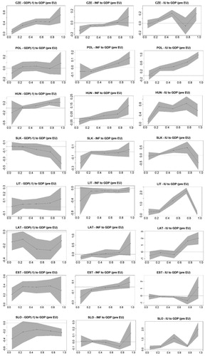
Figure A2. Graphical illustration of the estimated BQR parameters in the post-EU subperiod.

Note: see Figure 4.

References

- Alper, G. (2020). The impact of economic freedom on human development in European transition economies. Economic Computation and Economic Cybernetics Studies and Research, 54(3), 161–178. https://doi.org/10.24818/18423264/54.3.20.10
- Apergis, N. (2005). Inflation uncertainty and growth: Evidence from panel data. Australian Economic Papers, 44(2), 186–197. https://doi.org/10.1111/j.1467-8454.2005.00259.x
- Ball, L. (1992). Why does high inflation raise inflation uncertainty? Journal of Monetary Economics, 29(3), 371–388. https://doi.org/10.1016/0304-3932(92)90032-W
- Barndorff-Nielsen, O. E. (1997). Normal inverse Gaussian distributions and stochastic volatility modelling. Scandinavian Journal of Statistics, 24(1), 1–13. https://doi.org/10.1111/1467-9469.00045
- Benoit, D. F., & van den Poel, D. (2017). bayesQR: A Bayesian approach to quantile regression. Journal of Statistical Software, 76(7), 1–32. https://doi.org/10.18637/jss.v076.i07
- Berensmann, K., & BeyfuB, J. (2002). Central and Eastern Europe: Economic conditions ten years after the transformation. Romanian Journal of Economic Forecasting, 3(1), 49–61.
- Böhm, J., Filáček, J., Kubicová, I., & Zamazalová, R. (2012). Price-level targeting – A real alternative to inflation targeting? Finance a úvěr-Czech Journal of Economics and Finance, 62(1), 2–26.
- Buth, B., Kakinaka, M., & Miyamoto, H. (2015). Inflation and inflation uncertainty: The case of Cambodia, Lao PDR, and Vietnam. Journal of Asian Economics, 38, 31–43. https://doi.org/10.1016/j.asieco.2015.03.004
- Caglayan, M., Kocaaslan, O. K., & Mouratidis, K. (2016). Regime dependent effects of inflation uncertainty on real growth: A Markov switching approach. Scottish Journal of Political Economy, 63(2), 135–155. https://doi.org/10.1111/sjpe.12087
- Chang, K.-L., & He, C.-W. (2010). Does the magnitude of the effect of inflation uncertainty on output growth depend on the level of inflation? The Manchester School, 78(2), 126–148. https://doi.org/10.1111/j.1467-9957.2009.02162.x
- Chowdhury, K. B., Kundu, S., & Sarkar, N. (2018). Regime-dependent effects of uncertainty on inflation and output growth: Evidence from the United Kingdom and the United States. Scottish Journal of Political Economy, 65(4), 390–413. https://doi.org/10.1111/sjpe.12168
- Dotsey, M., & Sarte, P. D. (2000). Inflation uncertainty and growth in a cash-in-advance economy. Journal of Monetary Economics, 45(3), 631–655. https://doi.org/10.1016/S0304-3932(00)00005-2
- Engle, R. F., & Ng, V. K. (1993). Measuring and testing the impact of news on volatility. Journal of Finance, 48(5), 1749–1778. https://doi.org/10.1111/j.1540-6261.1993.tb05127.x
- Fischer, S. (1993). The role of macroeconomic factors in growth. Journal of Monetary Economics, 32(3), 485–512. https://doi.org/10.1016/0304-3932(93)90027-D
- Fountas, S. (2010). Inflation, inflation uncertainty and growth: Are they related? Economic Modelling, 27(5), 896–899. https://doi.org/10.1016/j.econmod.2010.06.001
- Friedman, M. (1977). Nobel lecture: Inflation and unemployment. Journal of Political Economy, 85(3), 451–472. https://doi.org/10.1086/260579
- Glosten, L., Jagannathan, R., & Runkle, D. (1993). Relationship between the expected value and the volatility of the nominal excess return on stocks. Journal of Finance, 48(5), 1779–1801. https://doi.org/10.1111/j.1540-6261.1993.tb05128.x
- Grier, R., & Grier, K. B. (2006). On the real effects of inflation and inflation uncertainty in Mexico. Journal of Development Economics, 80(2), 478–500. https://doi.org/10.1016/j.jdeveco.2005.02.002
- Grier, K. B., & Perry, M. J. (1998). On inflation and inflation uncertainty in the G7 countries. Journal of International Money and Finance, 17(4), 671–689. http://doi.org/10.1016/S0261-5606(98)00023-0
- Hasanov, M., & Omay, T. (2011). The relationship between inflation, output growth, and their uncertainties: Evidence from selected CEE countries. Emerging Markets Finance and Trade, 47(3), 5–20. https://doi.org/10.2753/REE1540-496X4704S301
- Hayford, M. D. (2000). Inflation uncertainty, unemployment uncertainty and economic activity. Journal of Macroeconomics, 22(2), 315–329. https://doi.org/10.1016/S0164-0704(00)00134-8
- Huang, H.-C., Yeh, C.-C., & Wang, X. (2019). Inflation targeting and output-inflation tradeoffs. Journal of International Money and Finance, 96, 102–120. https://doi.org/10.1016/j.jimonfin.2019.04.009
- Jiranyakul, K., & Opiela, T. P. (2011). The impact of inflation uncertainty on output growth and inflation in Thailand. Asian Economic Journal, 25(3), 291–307. https://doi.org/10.1111/j.1467-8381.2011.02062.x
- Kamber, G., & Wong, B. (2020). Global factors and trend inflation. Journal of International Economics, 122, 103265. https://doi.org/10.1016/j.jinteco.2019.103265
- Karilaid, I., & Talpsepp, T. (2014). Can policy improve liquidity during a financial crisis? Baltic Journal of Economics, 10(2), 5–26. https://doi.org/10.1080/1406099X.2010.10840476
- Koenker, R., & Bassett, G. (1978). Regression quantiles. Econometrica, 46(1), 33–50. https://doi.org/10.2307/1913643
- Li, W. K., & Mak, T. K. (1994). On the squared residual autocorrelations in non-linear time series with conditional heteroskedasticity. Journal of Time Series Analysis, 15(6), 627–636. https://doi.org/10.1111/j.1467-9892.1994.tb00217.x
- Lyziak, T. (2016). Survey measures of inflation expectations in Poland: Are they relevant from the macroeconomic perspective? Baltic Journal of Economics, 16(1), 33–52. https://doi.org/10.1080/1406099X.2016.1165402
- Maestri, V. (2013). Imputed rent and distributional effect of housing-related policies in Estonia. Italy and the United Kingdom. Baltic Journal of Economics, 13(2), 37–60.
- Njegić, J., Živkov, D., & Damnjanović, J. (2017). Business cycles synchronization between EU15 and the selected Eastern European countries – The wavelet coherence approach. Acta Oeconomica, 67(4), 539–556. https://doi.org/10.1556/032.2017.67.4.3
- Pagan, A. (1984). Econometric issues in the analysis of regressions with generated regressors. International Economic Review, 25(1), 221–247. https://doi.org/10.2307/2648877
- Pal, D., & Mitra, S. K. (2015). Impact of price realization on India’s tea export: Evidence from quantile autoregressive Distributed Lag model. Agricultural Economics - Zemedelska Ekonomika, 61(9), 422–428. https://doi.org/10.17221/209/2014-AGRICECON
- Pintilescu, C., Jemna, D.-V., Viorica, E.-D., & Asandului, M. (2014). Inflation, output growth, and their uncertainties: Empirical evidence for a causal relationship from European emerging economies. Emerging Markets Finance and Trade, 50(4), 78–94. https://doi.org/10.2753/REE1540-496X5004S405
- Svilokos, T., Vojinić, P., & Tolić, MŠ. (2019). The role of the financial sector in the process of industrialisation in Central and Eastern European countries. Economic Research-Ekonomska Istraživanja, 32(1), 384–402. https://doi.org/10.1080/1331677X.2018.1523739
- Usman, M., Jibran, M. A. Q., Amir-ud-Din, R., & Akhter, W. (2019). Decoupling hypothesis of Islamic stocks: Evidence from copula CoVaR approach. Borsa Istanbul Review, 19(S1), S56–S63. https://doi.org/10.1016/j.bir.2018.09.001
- Vilerts, K. (2018). The public-private sector wage gap in Latvia. Baltic Journal of Economics, 18(1), 25–50. https://doi.org/10.1080/1406099X.2018.1457356
- Wilson, B. K. (2006). The links between inflation, inflation uncertainty and output growth: New time series evidence from Japan. Journal of Macroeconomics, 28(3), 609–620. https://doi.org/10.1016/j.jmacro.2004.11.004
- Wu, J.-L., Chen, S.-L., & Lee, H.-Y. (2003). Sources of inflation uncertainty and real economic activity. Journal of Macroeconomics, 25(3), 397–409. https://doi.org/10.1016/S0164-0704(03)00045-4
- Žaček, J., Hruza, F., & Volčik, S. (2019). The impact of EU funds on regional economic growth of the Czech Republic. Finance a úvěr – Czech Journal of Economics and Finance, 69(1), 76–94.
- Živkov, D., Manić, S., Đurašković, J., & Kovačević, J. (2019). Bidirectional nexus between inflation and inflation uncertainty in the Asian emerging markets – the GARCH-in-mean approach. Finance a úvěr – Czech Journal of Economics and Finance, 69(6), 580–599.
- Živkov, D., Njegić, J., & Pećanac, M. (2014). Bidirectional linkage between inflation and inflation uncertainty – the case of Eastern European countries. Baltic Journal of Economics, 14(1–2), 124–139.
- Živkov, D., Pećanac, M., & Ercegovac, D. (in press). Interdependence between stocks and exchange rate in East Asia – A wavelet-based approach. Singapore Economic Review, https://doi.org/10.1142/S0217590819500450