An improved algorithm for dynamic nearest-neighbour models

ABSTRACT

The naïve algorithm for generating nearest-neighbour models determines the distance between every pair of nodes, resulting in quadratic running time. Such time complexity is common among spatial problems and impedes the generation of larger spatial models. In this article, an improved algorithm for the Mocnik model, an example of nearest-neighbour models, is introduced. Instead of solving $k$ nearest-neighbour problems for each node ($k$ dynamic in the sense that it varies among the nodes), the improved algorithm presented exploits the notion of locality through introducing a corresponding spatial index, resulting in a linear average-case time complexity.  This makes possible to generate very large prototypical spatial networks, which can serve as testbeds to evaluate and improve spatial algorithms, in particular, with respect to the optimization of algorithms towards big geospatial data.

KEYWORDS:

• Nearest-neighbour model
• kNN
• fixed-radius near neighbour
• Mocnik model
• spatial network
• spatial structure
• Tobler’s law

1. Introduction

Current data sources provide endless possibilities to engage in geospatial data production and analysis (Burke et al. 2006, Goodchild 2007, DeLyser and Sui 2012, Harvey 2013). Besides location, sensors in mobile phones measure tilt, acceleration, the magnetic field, temperature, proximity to human beings, ambient light, etc.; and they are able to record sound, images, and video. Also, social media provide information about our sentiments as well as verifiable information in the form of georeferenced text snippets (Stefanidis et al. 2013, Li et al. 2018). We often act and interact by means of digital technology, which makes us leaving digital traces that often incorporate the spatial dimension. Such information is special in the sense that the information is, to some degree, structured and shaped by space (Mocnik and Frank 2015, Mocnik 2015a, 2015b).

Some of the characteristics that make space can also be found in the thematic dimensions of the data, i.e., on the dimensions referring to the ‘what’ instead of the ‘where’ or ‘when’. This is because spatial and the thematic aspects are often interdependent and interwoven. Thereby, thematic information inherits some of the properties of space, most importantly, the notion of locality: things can exist or happen in the same vicinity. Space provides thus structure to thematic information, which is why we are able to perform spatial queries and relate things by their position in space.

Spatial and geographical information can, in many cases, formally be conceptualized as networks (Barabási and Bonabeau 2003, Holme and Saramäki 2012) and often be modelled by nearest-neighbour models (Aldous and Ganesan 2013, Mocnik and Frank 2015, Mocnik 2015b). The class of such nearest-neighbour models can be described by simple rules, but generating such a network is often computationally intensive. In fact, when generating the network using the naïve algorithm, the nearest neighbours have to be determined for each node of the network. The running time is thus of average-case time complexity $O(n\cdot C(n))$, where $O(C(n))$ is the complexity of finding, for a given node, all its neighbouring nodes. For determining the neighbouring nodes, the naïve algorithm would check for each node the distance to all other nodes, yielding an overall average-case time complexity of $O(n^2)$. For finding neighbouring nodes more efficiently, an index can be used, yielding an overall complexity lower than $O(n^2)$ but still higher than $O(n)$.

This article focuses on a particular example of nearest-neighbour models, the Mocnik model (Mocnik and Frank 2015, Mocnik 2015b, 2018b). Given the parameters needed to generate the model, i.e., the number of nodes $n$, the dimension $d$, and the parameter $\rho$, we seek for an algorithm that generates an instance of the corresponding Mocnik model as efficient as possible – with minimal time complexity. In this article, we present an algorithm that is able to compute the Mocnik model in linear time, i.e., in average-case time complexity $O(n)$, which is much faster compared to the naïve algorithm with complexity $O(n^2)$. The linear complexity is similar to solutions of the fixed-radius near neighbour search problem (Bentley 1975b, Bentley et al. 1977), but as the Mocnik model assumes no fixed radius, a variant with a spatial index needs to be employed. Such linear average-case time complexity is possible because the generation of the Mocnik model can be performed locally. As a result, larger Mocnik models can easily be generated.

The article is organized as follows. First, we briefly discuss spatial networks (Section 2.1) and nearest-neighbour models (Section 2.2) by setting them into the context of existing literature. In particular, the Mocnik model is discussed as an example of a nearest-neighbour model. Then, we discuss the fixed-radius near neighbour search problem, including its variants like the $k$ nearest-neighbour search problem (Section 2.3). These techniques can be used to generate nearest-neighbour models efficiently. This is, however, not possible for the Mocnik model, because the model is dynamic in the sense that edges are determined by the mutual relative distances of the involved nodes. After a short discussion of the naïve algorithm for generating a Mocnik model (Section 3.1), we examine how to utilize a spatial grid as a spatial index (Section 3.2). This spatial index, in turn, renders possible to generate both non-hierarchical and hierarchical Mocnik models in linear time, which is demonstrated by a novel improved algorithm (Section 3.3 and Section 3.4). The improved algorithm is successfully evaluated by showing that its average-case complexity is linear in the number of nodes of the network (Section 4). Finally, we reflect on the opportunities the efficient generation of a Mocnik model offers in the context of big geospatial data (Section 5). The algorithm for generating the locations of the nodes (Appendix A) and algorithms related to the spatial grid (Appendices B and C) can be found annexed to the end of the article. Finally, empirical running time series about the influence of the dimension of the embedding space and the parameter $\rho$ on running times is annexed (Appendix D).

2. Related work

This section provides an overview of existing literature on spatial networks in general, as well as nearest-neighbour models and the Mocnik model in particular. Also, the literature on the fixed-radius near neighbour search problem and its variants are discussed.

2.1. Spatial networks

In various fields, the structure of information has been formally described and examined by the use of networks (Barabási and Bonabeau 2003, Holme and Saramäki 2012). Among these examples are the structure of social interaction and social links (Holland and Leinhardt 1981, Onnela et al. 2007, Hunter et al. 2008, Sala et al. 2010), computer networks and the World Wide Web (Albert et al. 1999, Barabási and Albert 1999, Barabási et al. 2000, Yook et al. 2002), scientific collaboration networks (Newman 2001, Barabási et al. 2002), transport and road networks (Kalapala et al. 2006, Louf et al. 2014), economic networks in the context of geography (Baum et al. 2003, Glückler 2007), brain networks (Sporns et al. 2005, Bullmore and Sporns 2009, van den Heuvel et al. 2012), genetic networks (Barabási and Albert 1999), networks describing the spread of diseases (Watts and Strogatz 1998), and many more. The structural view offered by networks is a suitable approach to explore extensive data sets and big geospatial data.

The specific characteristics of spatial networks have, among others, been examined by an analysis of volumes in the network. Such a volume is defined as the number of nodes being reachable from a centre node by a fixed number of edges. The volume in a network has, e.g., been utilized for understanding how space shapes thematic structure (Mocnik 2015b, 2018a). In particular, it has been shown that the volume in a spatial network often statistically scales in the same way as the volume in space, known as the polynomial volume law of spatial networks (Mocnik 2018b): if a network is placed in and strongly shaped by a $d$-dimensional space, volumes in the network scale as $r^d$. It has even been demonstrated that the dimension of the embedding space can be reconstructed from the abstract network by the analysis of volumes in the network (Mocnik 2018b). Knowledge about the dimension of a network can, e.g., be used for classifying networks and for building corresponding search engines for networks. Also, further characteristics of spatial networks have been discussed (Barthélemy 2011).

Space is one of the major factors that shape networks. Besides the analysis of real-world networks, several models of spatial networks have thus been introduced. While planar networks are an important class of networks (Kuratowski 1930, Whitney 1931, MacLane 1937, Wagner 1937), they describe only networks that can ideally be embedded in space. Geographical reality does though not enforce networks to be prototypical spatial but instead combines spatial and thematic dimensions. Networks, the nodes of which are embedded in geographical space, have been discussed by Haggett and Chorley (1969). Spatial networks, in general, have been discussed by Barthélemy (2011). An important class of spatial networks are nearest-neighbour models, the nodes of which are adjacent in the network if they are also neighbouring in space. These models differ in the way the neighbours of a node are determined. Among these models are the Waxman model, which makes use of a probability function (Waxman 1988); a model introduced by Huttenhower et al. (2007); and a model introduced by Aldous and Shun (2010). The latter one is scale-invariant, a property discussed by Aldous and Ganesan (2013). Another example of a nearest-neighbour model is the Mocnik model (Mocnik and Frank 2015, Mocnik 2015b, 2018b). However, all types of nearest-neighbour models can be used to test algorithms and workflows on large spatial networks, creating the need to algorithmically generate such networks very efficiently.

2.2. Nearest-neighbour models and the Mocnik model

Tobler’s First Law of Geography can be found within many contexts and in many data sets. Geographical features are scattered in space, sometimes in a uniform way, but usually, the features expose patterns or even cluster to some degree. In many cases and oftentimes independent of how features are arranged, Tobler’s First Law of Geography applies: ‘near things are more related than distant things’ (Tobler 1970). This law implies that geographical influences are often of local nature. The complexity of geographical systems is accordingly limited by the fact that strong influences often happen in spatial neighbourhoods. In addition to the notion of locality found in geographical systems, geographical context goes much beyond the local neighbourhood. Tobler’s First Law accordingly also states that ‘everything is related to everything else’ (Tobler 1970), which, in turn, means that a restriction to limited neighbourhoods is often inadequate for geographical analysis and discussion. A similar effect is described by Tobler’s Second Law of Geography, which states that a ‘phenomenon external to an area of interest affects what goes on in the inside’ (Tobler 1999). Tobler’s laws have been widely acknowledged as being fundamental to geographical research (Barnes 2004, Goodchild 2004, Miller 2004, Phillips 2004, Smith 2004, Sui 2004, Tobler 2004, Westlund 2013). Also, the often local nature of geographical influence, complemented by the high complexity of geographical systems, has been widely discussed in publications (Anselin 1995, Hecht and Moxley 2009, Westerholt et al. 2016, Mocnik 2018c).

Nearest-neighbour models (Waxman 1988, Huttenhower et al. 2007, Aldous and Shun 2010, Aldous and Ganesan 2013, Mocnik and Frank 2015, Mocnik 2015b, 2018b) often resemble Tobler’s First Law of Geography in prototypical ways. These models have in common that nodes are adjacent in the network if they are, in some way, near in space. They differ, however, by the way the nearest nodes are determined. The Mocnik model (Mocnik and Frank 2015, Mocnik 2018b), which is examined as an example in this article, has properties that are of particular interest to geography. Among these properties is the fact that edges are introduced independently of scale (Mocnik 2015b). The idea of the model is straightforward. For a given set of nodes that are placed in a $d$-dimensional Euclidean space, edges are introduced between nodes in the same vicinity. Thereby, a directed edge between nodes $n_1$ and $n_2$ is introduced if and only if

(1) $\mathrm{d}\mathrm{i}\mathrm{s}\mathrm{t}(n_1,n_2)\le \rho \cdot \underset{m\ne n_1}{min}\mathrm{d}\mathrm{i}\mathrm{s}\mathrm{t}(n_1,m)$(1)

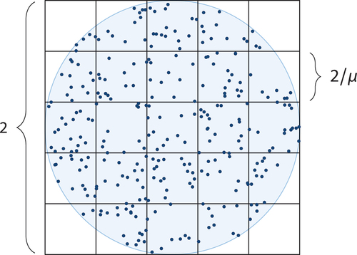
where $m$ is the node being nearest to node $n_1$, and $\rho >1$ is a parameter influencing the density of the network, i.e., the number of edges added to each node. Instead of using a set of given locations, as in Figure 1, nodes are often randomly distributed in the $d$-dimensional unit ball with a uniform distribution. Numerous instances of such Mocnik models with randomly distributed nodes exist, which is why we speak of ‘an instance of the Mocnik model’ or ‘a Mocnik model’ in this case. In the scope of this article, we assume such randomly distributed nodes in the unit ball for instances of the Mocnik model.

Figure 1. Different networks, the nodes N of which are the stops of the national railway operator SJ in Sweden. (a) Network representation of the original network, (b) the Mocnik model for the nodes $N$ and $\rho =2$, and (c) a Gilbert model (Gilbert 1959) for the nodes $N$ and probability ${10}^{-3}$. The parameters are chosen such that similarities and dissimilarities visually stand out.

The Mocnik model is a result of local optimization (Mocnik 2018b). Real networks are, however, often to some degree guided by global optimization as well. Road networks, e.g., consist of many edges that connect nodes being near in space, optimizing for local distances. At the same time, some of these edges allow for larger travel speed, such as highways, thereby connecting more distant nodes. Such local and global optimization typically coexists in geographical networks, which is why the hierarchical Mocnik model has been introduced (Mocnik 2018b). The hierarchical model consists of different layers. These layers are constituted by node sets $N_l\subset N_{l-1}\subset \dots \subset N_1\subset N_0$ with a growing number of nodes, where $N_l$ refers to the nodes of the top layer and $N_0$ to the nodes of the base layer. Each of these layers is, per definition, the Mocnik model of the corresponding set of nodes. The resulting overall network consists thus of many edges between nodes of the same vicinity and some additional shortcuts between more distant nodes.

The generation of nearest-neighbour models, such as the Mocnik model, poses computational challenges. The naïve approach to the generation of such a model needs to consider all pairs of nodes when computing their distances. The quadratic complexity of the naïve algorithm derives from the fact that the distance needs to be computed even for pairs of very distant nodes. The same quadratic complexity applies to other cases in which binary functions shall be evaluated for all elements of a system, e.g., when determining the Egenhofer relations (Egenhofer 1991) between all pairs of spatial regions in a data set, or when applying Allen’s interval algebra (Allen 1983) to temporal intervals. As a result, the creation and reasoning with qualitative spatial relations for a large number of objects become inefficient (Fogliaroni 2013).

The complexity of generating nearest-neighbour models for a larger set of nodes can be reduced when exploiting the notion of locality. In spatial networks, ‘being near in space’ and ‘being adjacent in the network’ often correlates (near-in-space–near-in-network condition). As shortcuts do not exist in space – this would contradict the triangle inequality – shortcuts do not exist in nearest-neighbour models either in the same extent as in other networks. In a nearest-neighbour model, balls with a small radius do thus not exhaust the network. One is rather able to distinguish between different neighbourhoods, which is in contrast to small-world networks, such as many social networks. In these, two arbitrary nodes are usually related by only a small number of edges. If one starts at an arbitrary user profile on Facebook and follows four friendship links (all of them), one will have visited almost every user profile in this social network (Backstrom et al. 2012). Accordingly, using such techniques for reducing the complexity by exploiting the near-in-space–near-in-network condition and thus focussing on small neighbourhoods only does not work in such small-world networks. If a network, however, inherits some notion of locality, the number of considered pairs of nodes can be reduced. In the following section, means to address the complexity by exploiting the near-in-space–near-in-network condition are discussed.

2.3. The fixed-radius near neighbour search problem and variants

The naïve algorithm for generating a nearest-neighbour model can easily be improved with respect to its efficiency by making use of the notion of locality, which is inherent to space and thus also to nearest-neighbour models. When generating a nearest-neighbour model in a naïve way, each node is successively considered. For each such node, a nearest neighbour search problem (also known as the ‘post office problem’, Knuth 1973) needs to be performed by determining the distance to every other node and then introducing edges to each node being near. This approach results in considering every pair of nodes at least once and has thus a complexity of $O(n^2)$. When making use of the near-in-space–near-in-network condition, i.e., of the notion of locality, better running times can be achieved, as is discussed in the remainder of this section.

A generalization of the near neighbour search problem, the fixed-radius near neighbour search problem, has been discussed by Levinthal (1966) and Bentley (1975b). This problem asks for all nodes within a fixed radius rather than only for the nearest node. A corresponding nearest-neighbour network model, in which nodes are adjacent if they are within a fixed distance in space, has been introduced by Aldous and Shun (2010). As the nearest nodes can be searched for in parallel, algorithmic solutions are much more efficient than when computing the distance of all pairs of nodes. By using hash tables (Bentley et al. 1977) or by partitioning space in cells related to the corresponding radius (Mattson and Rice 1999), the fixed-radius near neighbour search problem can be solved in linear time in the optimal case. The generation of the network model is thus of complexity $O(n)$ too.

Another variant is the nearest-neighbour model, in which every node is adjacent to the $k$ nearest nodes. Instead of computing the distance in space to each other node, a spatial index can be used. Existing spatial indexing methods usually expose (in the optimal case) logarithmic complexity for querying the nearest neighbour, as is the case when using an R tree (Guttman 1984, Cheung and Fu 1998), its variant of an R* tree (Beckmann et al. 1990), or further variants (Roussopoulos and Leifker 1985, Kamel and Faloutsos 1994); when introducing cells of different size and building a corresponding quad-tree (Finkel and Bentley 1974); when partitioning space and building a corresponding k-d tree (Bentley 1975a, Friedman et al. 1977); when partitioning space using PMR quadtrees (Nelson and Samet 1987, Hjaltason and Samet 1995); or when using SS-trees (White and Jain 1996, Kurniawati et al. 1997). For the corresponding network model, the use of such a spatial index would improve running time to $O(nlogn)$ at best if the number of considered neighbours remains constant.

Further algorithms address the $k$ nearest neighbour search problem, i.e., the problem of finding the $k$ nearest neighbours of a node, thereby being tailored to different requirements. For instance, solutions to the search problem have been optimized for high dimensional space (ERkNN, Xia et al. 2005) and with respect to reverse search (Figueroa and Paredes 2009). The search problem has also been explored with respect to networks (Figueroa and Paredes 2009). When performing several searches, preprocessing the data can improve overall running time (Zhong et al. 2017). Probabilistic approaches can cope more efficiently with higher dimensionality while still providing logarithmic performance with respect to the number of nodes (Weiss 1980). The efficiency of probabilistic approaches can even be increased when preprocessing the data, as has been discussed at the example of the AESA algorithm (Vidal 1994) and its improved variants LAESA (Micó et al. 1994), TLAESA (Micó et al. 1996), and an improved TLAESA algorithm (Tokoro et al. 2006). Further variants of the aforenamed strategies exist (Sproull 1991, Roussopoulos et al. 1995). It has even been shown that solutions of the fixed-radius near neighbour search problem can be adapted to also solve the $k$ nearest neighbour search problem (Gao et al. 2015). Many of these algorithms are sublinear in the number of nodes, still resulting in an overall running time of complexity larger than $O(n)$ when generating a Mocnik model.

In contrast to the discussed variants of nearest-neighbour models, the adjacent nodes of a node in the Mocnik model are not within a fixed radius of the latter, and their number is neither constant nor restricted. Whether two nodes are adjacent in the Mocnik model rather depends on their relative distances. In this way, the Mocnik model is an example of a dynamic nearest-neighbour model, in which neither the number of adjacent nodes nor the radius is fixed in the above sense. This is why existing strategies for efficiently generating such a network cannot be used. As has been discussed by Mocnik (2015b) this difference is of importance for modelling geographical systems. In the next section, we discuss an improved algorithm for generating the Mocnik model, which makes use of a spatial index and thus exploits the notion of locality. The algorithm has a complexity of $O(n)$, which is comparable to highly optimized solutions for generating nearest-neighbour models related to the fixed-radius near neighbour search problem.

3. Algorithms for generating the Mocnik model

This section discusses two algorithms to generate an instance of the Mocnik model: a naïve one in the first subsection, and an improved, much more efficient version in subsequent sections. The improved efficiency of the latter is achieved by partitioning space into cells and using these cells as a spatial index, as is a common approach (Finkel and Bentley 1974, Mattson and Rice 1999). By choosing a suitable cell size, the overall average-case complexity of the algorithm can thus be reduced to $O(n)$. Both the naïve and the improved algorithm are part of NetworKit (Staudt et al. 2016), an open-source toolkit for large-scale network analysis.¹ Further improvements concerning running time can be achieved by minor changes, among others, by using global variables instead of local ones, by changing the order of conditions, etc. These improvements do, however, not change the complexity of the algorithms and strongly depend on the programming language, the compiler, and the hardware being used, which is why a discussion of these improvements is not included in this article. The algorithms in NetworKit have been further optimized.

In subsequent subsections, the naïve algorithm (Algorithm 1) and the improved algorithm (Algorithm 2) are provided. These algorithms make use of algorithms provided in the appendix – an algorithm to place the nodes in the unit ball (Algorithm A1, Appendix A), algorithms for indexing the nodes in a spatial grid (Algorithm B1 and B2, Appendix B), and algorithms for finding neighbouring cells in the spatial grid (Algorithm C1 and C2, Appendix C). An overview of the various time complexities of these algorithms is provided in Table 1. As the complexity of the improved algorithm strongly depends on the random distribution of the nodes, practical running times can differ. We thus focus on the average-case complexity (Levin 1986) of the algorithms.

Table 1. Average-case time complexity of the algorithms discussed in this article. Algorithm 1 is the naïve and Algorithm 2 the improved algorithm for generating a Mocnik model. As Algorithms A1–C2 are of supplementary nature (they are used by Algorithms 1 and 2) they are discussed in the appendix. The complexity refers to the dimension $d$, the number of nodes $n$, the parameter $\rho$ of the Mocnik model, and, in case of Algorithms C1 and C2, to the radius r used in the algorithm. In Algorithm 2, the typical radius $\tilde{r}$ is a constant.

Algorithm	Complexity	Complexity (d and $\mathit{\rho }$ const.)
Algorithm 1	$O(d\cdot n^2+d\cdot (2/\sqrt{\pi }{)}^d\cdot \mathrm{\Gamma }(d/2+1)\cdot n)$	$O(n^2)$
Algorithm 2	$O(d\cdot (2/\sqrt{\pi }{)}^d\cdot \mathrm{\Gamma }(d/2+1)\cdot n+d\cdot {\rho }^d\cdot (2\tilde{r}{)}^d\cdot n)$	$O(n)$
Algorithm A1	$O(d\cdot (2/\sqrt{\pi }{)}^d\cdot \mathrm{\Gamma }(d/2+1)\cdot n)$	$O(n)$
Algorithm B1a	$O(d)$	$O(1)$
Algorithm B1b	$O(d)$	$O(1)$
Algorithm B2	$O(d)$	$O(1)$
Algorithm C1	$O(d\cdot (2r{)}^d)$	$O(r^d)$
Algorithm C2	$O(d^2\cdot (2r{)}^{d-1})$	$O(r^{d-1})$

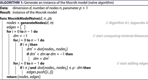
3.1. The naïve algorithm

An algorithm for generating a Mocnik model obviously has to incorporate the following parts: first, the generation of the nodes including their coordinates; secondly, the determination of the distance to the nearest node for each of the nodes; and thirdly, the generation of the edges. An algorithm for generating nodes randomly distributed in a unit ball with uniform distribution is provided as Algorithm A1 (Appendix A).

After the generation of the nodes, the naïve algorithm of the Mocnik model (Algorithm 1) successively considers each node. For each such node, the nearest neighbour is determined. Then, the distances to all other nodes are computed. In case that Equation 1(1) $\mathrm{d}\mathrm{i}\mathrm{s}\mathrm{t}(n_1,n_2)\le \rho \cdot \underset{m\ne n_1}{min}\mathrm{d}\mathrm{i}\mathrm{s}\mathrm{t}(n_1,m)$(1) is satisfied, a corresponding edge is introduced. While this approach is straightforward, it scales badly. Both parts, the determination of the nearest neighbour and the checking whether Equation 1(1) $\mathrm{d}\mathrm{i}\mathrm{s}\mathrm{t}(n_1,n_2)\le \rho \cdot \underset{m\ne n_1}{min}\mathrm{d}\mathrm{i}\mathrm{s}\mathrm{t}(n_1,m)$(1) is satisfied, use two nested loops for finding all pairs of nodes. For each such pair of nodes, the distance is determined. As the computation of the distance is of complexity $O(d)$, the overall complexity of these two steps is $O(d\cdot n^2)$. For a fixed dimension, the naïve Algorithm 1 is thus of quadratic complexity (Table 1).

3.2. Indexing by a spatial grid

In order to improve the naïve algorithm and achieve much lower complexity with respect to the running time, the nodes will be indexed in a spatial grid. This allows to access nodes in the same vicinity efficiently and, ultimately, to generate a Mocnik model in linear average-case running time. In this section, we provide an overview of the algorithms used for the indexing (Table 2). The algorithms themselves are annexed in the appendix.

Table 2. Algorithms related to the index and the spatial grid. The algorithms refer to the dimension $d$ of the space as well as to the number of grid cells per dimension $\mu$.

Algorithm	Symbol	Output
Algorithm B1a	toID$(c,\mu )$	ID ι of the grid cell with integer coordinates $c$
Algorithm B1b	fromID$(\iota ,d,\mu )$	integer coordinates $c$ of the grid cell with ID $\iota$
Algorithm B2	determineGridCell$(\nu ,\mu )$	ID of the grid cell containing the pair of coordinates $\nu$
Algorithm C1	volumeOfCube$(\iota ,r,d,\mu )$	IDs of the grid cells forming the hypercube centred at $\iota$ and with a radius of $⌈r⌉$
Algorithm C2	surfaceOfCube$(\iota ,r,d,\mu )$	IDs of the grid cells forming the surface of the hypercube centred at $\iota$ and with a radius of $r$

The nodes generated by Algorithm A1 (Appendix A) are contained in the unit ball and thus also in the cube of edge length 2. By grouping the nodes into spatial neighbourhoods, they can easily be retrieved when searching for neighbouring nodes. For this purpose, each edge of the cube is subdivided into $\mu$ parts, thereby creating ${\mu }^d$ grid cells with an edge length of $2/\mu$ (Figure 2). These grid cells function as the spatial neighbourhoods of our spatial index. Each node is thereby assigned to the cell it is contained in. When querying for the nodes contained in some neighbourhood, only the nodes contained in the corresponding grid cells need to be considered. All other grid cells and their corresponding nodes can be ignored.

Figure 2. Spatial grid for indexing nodes. The grid consists of ${\mu }^d$ cells, where $d$ is the dimension and $\mu$ an integer. Each cell is of edge length $2/\mu$.

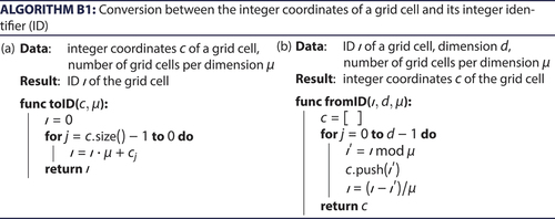
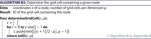
The cells of the spatial grid are identified by integer coordinates. Each of the cells is thereby referred to by a $d$-tuple of integer values, ranging from $0$ to $\mu -1$ when being in $d$-dimensional space. While such integer coordinates are a natural choice, they can in most programming languages not be used as an index of a vector. Such a vector is, however, needed to store the nodes grouped by the grid cells. The function toID (Algorithm B1a, Appendix B) provides a mapping from the integer coordinates of a grid cell to an integer number, acting as an integer identifier (ID). The inverse function fromID (Algorithm B1b, Appendix B) accordingly provides for an ID, i.e., an integer number, the corresponding integer coordinates (Figure 3). Finally, the function determineGridCell (Algorithm B2, Appendix B) determines for a given pair of coordinates of a node the ID of the corresponding grid cell, as is needed for indexing the node.

Figure 3. Identifiers (IDs) for the spatial grid. The function toID translates from integer coordinates to IDs, while the function fromID translates into the opposite direction.

The improved algorithm utilizes the spatial grid introduced above for efficiently finding neighbouring nodes. Assume that the spatial grid has ${\mu }^d$ cells and is contained in $d$-dimensional space. Further assume that we search nodes neighbouring a given node, which is contained in a grid cell $\iota$. Then, these neighbouring nodes are contained in the cells adjacent to grid cell $\iota$ if they are within a distance of $2/\mu$ – each cell has an edge length of $2/\mu$. 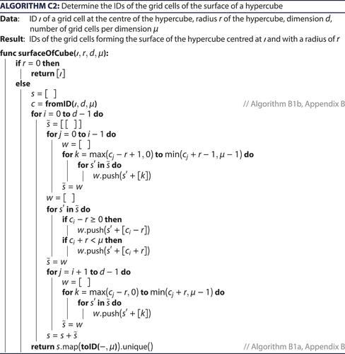The adjacent grid cells, together with the grid cell $\iota$, form a hypercube of radius $1$ within the spatial grid. When nodes within a larger distance shall be found, hypercubes of larger radii need to be considered. The function volumeOfCube (Algorithm C1, Appendix C) computes for a given centre node $\iota$ and a given radius $r$ the grid cells contained in the corresponding hypercube. 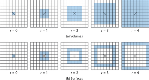In addition, the function surfaceOfCube (Algorithm C2, Appendix C) computes the grid cells at distance $r$ to a given centre node $\iota$, i.e., the grid cells of the surface of the hypercube (Figure 4).

Figure 4. Volumes and surfaces in the spatial grid. (a) Volumes in the spatial grid, marked in blue, form hypercubes of adjacent cells. They are determined by their centre cell, here marked by a cross, and their radius. The volume at radius $r$ is contained in the volume of radius $r+1$. (b) The surface at radius $r$ is the volume at radius $r$ with the volume at radius $r-1$ removed.

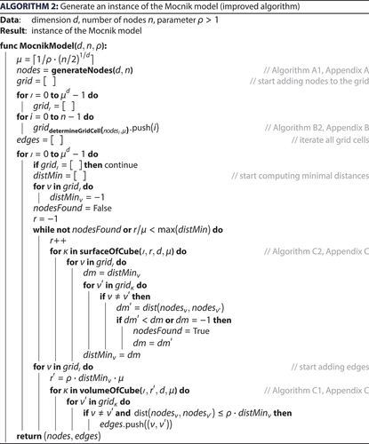
3.3. The improved algorithm

Having established methods to index nodes by a spatial grid and to determine neighbourhoods in the grid, we can improve the algorithm for generating a Mocnik model. The use of the spatial grid discussed in the previous section makes the algorithm much more efficient in comparison to the naïve algorithm, because it renders possible to exploit the locality of the resulting network. Thereby, the algorithm only compares nodes that are near each other in space and avoids unnecessary computations.

The improved algorithm for generating a Mocnik model, Algorithm 2, generates the nodes, including their coordinates, in the same way as the naïve algorithm does. For doing so, it again uses Algorithm A1 (Appendix A). In a second step, the improved algorithm assigns the nodes to a spatial grid, which acts as an index in the way described above. In the third step, the required distances between nodes are finally determined to then add corresponding edges. For doing so, the algorithm iterates through the grid cells and their corresponding nodes. For each grid cell $\iota$, it considers the distances to all nodes of the grid cell itself ($r=0$), to the nodes of adjacent grid cells ($r=1$), and the nodes in further grid cells ($r=2$, etc.), until a nearest node is found for each node of the original grid cell (Algorithm C2, Appendix C). These minimum distances are then used to find all edges starting at a node of the considered grid cell, which requires to examine all nodes in the grid cells of the corresponding hypercube (Algorithm C1, Appendix C).

The size $\mu$ of the spatial grid has an impact on the running time. Ideally, we try to achieve $O(n)$ running time by choosing a suitable $\mu$, which means to keep constant the number of grid cells that is to be considered in each iteration step – the determination of the nearest neighbour for each node and the addition of edges. The number of nodes per cell should thus be independent of the overall number of nodes $n$. The $d$-dimensional spatial grid with a side length of $\mu$ consists of ${\mu }^d$ cells. Each grid cell contains thus $n/{\mu }^d$ nodes on average. If this number is to be kept constant at value $c$, the side length $\mu$ equals $(n/c{)}^{1/d}$. This choice ensures that the average number of grid cells to consider when finding the nearest neighbouring nodes remains constant, independent of the overall number of nodes.

The parameter $\rho$ influences the density of the network. For larger $\rho$, the network has more edges. While the minimal distances are independent of $\rho$ – the same number of nodes is contained in the same amount of space – the average number of edges starting at each node converges to ${\rho }^d$ for $n\to \mathrm{\infty }$ and is thus practically independent of the overall number of nodes contained in the network, as has been shown by Mocnik and Frank (2015) and Mocnik (2015b). Accordingly, the number of grid cells to be considered when adding edges would grow for increasing $\rho$. To keep this number constant, however, the number of nodes contained in each grid cell needs to be proportional to ${\rho }^d$ on average, and $\mu$ equals accordingly $1/\rho \cdot (n/c{)}^{1/d}$. This, in turn, means that for growing $\rho$ the grid becomes more coarse, which practically increases the running time slightly. Despite the fact that the choice of $c\gg 1$ does not impact the complexity, the choice has a practical impact on the running time. A value of $c=2$ seems to be a reasonable choice.

The improved algorithm needs to generate the coordinates for the nodes, which is of complexity $O(d\cdot (2/\sqrt{\pi }{)}^d\cdot \mathrm{\Gamma }(d/2+1)\cdot n)$, as is shown in Appendix A. Thereafter, the algorithm consecutively examines nodes in $n/(2{\rho }^d)$ grid cells. In each of the grid cells, the grid cells of a hypercube of some radius $\tilde{r}$ are examined. The determination of the grid cells of this hypercube is of complexity $O(d\cdot (2\tilde{r}{)}^d)$, as is discussed for Algorithm C1 in Appendix C, yielding $O((2\tilde{r}{)}^d)$ grid cells. By the choice of $\mu$ and thus the average number of nodes in a grid cell, the average radius $\tilde{r}$ is kept constant. Further, the algorithm to determine the edges contains two nested loops that each iterate through the $2{\rho }^d$ nodes (on average) of a grid cell. Finally, the distance function is of complexity $O(d)$. When computing the overall complexity of the improved algorithm, it should be noted that the computation of the minimal distances is faster than the computation of the edges. Accordingly, the overall complexity of the improved algorithm is determined by the complexity of Algorithm A1 (Appendix A), the number of grid cells, the number of grid cells of the hypercube, the two loops, and the distance function. A short computation shows that the overall average-case time complexity of Algorithm 2 is given as

$O(d\cdot (2/\sqrt{\pi }{)}^d\cdot \mathrm{\Gamma }(d/2+1)\cdot n+d\cdot {\rho }^d\cdot (2\tilde{r}{)}^d\cdot n).$

For a fixed dimension $d$ and fixed $\rho$, the average-case time complexity is thus $O(n)$.

3.4. Hierarchical model

The hierarchical Mocnik model consists of several Mocnik models, which is why it can be created in a very similar way. Again, the improved algorithm can be used. In the first step, nodes are created as before. In subsequent steps, the improved Algorithm 2 is executed for each layer of the hierarchy. Thereby, the generation of nodes can, of course, be omitted. Instead of new nodes, the first $n_i$ nodes are chosen for the $i$-th layer and the algorithm can be executed as before. The same edge can occur in different layers, which creates the need to remove duplicate edges after running the algorithm.

We have discussed an algorithm to generate instances of the Mocnik model. Both in the non-hierarchical and the hierarchical variant, the average-case time complexity is $O(n)$, as has been argued. In the following section, we will evaluate the running time of the non-hierarchical model empirically. As the hierarchical model consists of several non-hierarchical models, the running times add up, which is why an empirical evaluation of the hierarchical model is not necessary.

4. Empirical running time evaluation

The naïve algorithm for generating a Mocnik model can be seen as a special case of the improved algorithm. The improved algorithm makes use of a spatial grid that allows for exploiting the locality of the network. If the entire grid consists of one grid cell only, the improved algorithm resembles the naïve one. The choice of an optimal number of grid cells, as is the case in Algorithm 2, makes the algorithm much more efficient in the average case. If all nodes are, by chance, in the same grid cell, the improved algorithm will, however, run about as long as the naïve one. In this section, we will thus evaluate running times empirically.

The evaluation of the algorithms has been performed on a MacBook Pro (13-inch, 2019, 2.8 GHz Intel Core i7 CPU, 16 GB 2133 MHz LPDDR3 memory) running macOS 10.15.2, Python 3.7.5, Clang 1100.0.33.17, and an unmodified version of NetworKit 6.0. Prior to each test, in which an instance of the Mocnik model is generated, the library NetworKit was preloaded. Then, all tests were performed five times in a row, and the shortest running time was selected. The running times are provided in Table 3.

Table 3. Running times of the naïve and the improved algorithm. The running times refer to the generation of a Mocnik model with parameter $\rho =1.6$. All times are given in seconds.

	d = 2			d = 3
Number of nodes	Naïve	Improved	Improved parallel	Naïve	Improved	Improved parallel
5.0·10^2	2.16·10^−^3	5.19·10^−^3	3.02·10^−^3	2.60·10^−^3	1.05·10^−^2	6.14·10^−^3
1.0·10^3	6.58·10^−^3	9.57·10^−^3	6.24·10^−^3	8.90·10^−^3	2.52·10^−^2	1.39·10^−^2
2.5·10^3	4.11·10^−^2	2.70·10^−^2	1.54·10^−^2	4.47·10^−^2	6.25·10^−^2	3.59·10^−^2
5.0·10^3	1.47·10^−^1	5.31·10^−^2	2.86·10^−^2	1.72·10^−^1	1.24·10^−^1	7.12·10^−^2
7.5·10^3	3.11·10^−^1	8.34·10^−^2	4.23·10^−^2	3.73·10^−^1	1.88·10^−^1	1.08·10^−^1
1.0·10^4	5.76·10^−^1	1.00·10^−^1	5.82·10^−^2	6.59·10^−^1	2.56·10^−^1	1.44·10^−^1
2.5·10^4	3.37·10^0	2.49·10^−^1	1.45·10^−^1	3.91·10^0	6.53·10^−^1	3.57·10^−^1
5.0·10^4	1.31·10^1	5.02·10^−^1	2.89·10^−^1	1.47·10^1	1.29·10^0	7.18·10^−^1
7.5·10^4	2.83·10^1	7.36·10^−^1	4.39·10^−^1	3.31·10^1	1.91·10^0	1.14·10^0
1.0·10^5	5.05·10^1	9.79·10^−^1	6.21·10^−^1	6.01·10^1	2.56·10^0	1.52·10^0
2.5·10^5	3.46·10^2	2.50·10^0	1.56·10^0	3.99·10^2	6.53·10^0	3.84·10^0
5.0·10^5	1.36·10^3	5.13·10^0	3.21·10^0	1.62·10^3	1.32·10^1	7.94·10^0
7.5·10^5	3.07·10^3	7.88·10^0	4.93·10^0	3.58·10^3	1.98·10^1	1.19·10^1
1.0·10^6	5.26·10^3	1.05·10^1	6.62·10^0	6.19·10^3	2.80·10^1	1.58·10^1

The comparison of the naïve and the improved algorithm does reveal not only a quantitative difference in running times but also a qualitative one. As becomes apparent in Figure 5, the improved algorithm is much more efficient than the naïve one. Only for networks with some hundred nodes, running times are of the same order of magnitude. The improved algorithm is about 5.8 times faster for 10,000 nodes distributed in the unit ball in two-dimensional space, 51.6 times faster for 100,000 nodes, and 50.1 times faster for 1,000,000 nodes. In three-dimensional space, the improved algorithm is about 2.6 times faster for 10,000 nodes, 23.5 times faster for 100,000 nodes, and 221.1 times faster for 1,000,000 nodes. It can be seen from Figures 5 and 6 that the running time of the naïve algorithm scales quadratically while the running time of the improved algorithm is near to linear.

Figure 5. Running times of the naïve and the improved algorithm for generating a Mocnik model ($\mathit{\rho }\mathbf{=}\mathbf{1}\mathbf{.6}$). (compare Table 3)

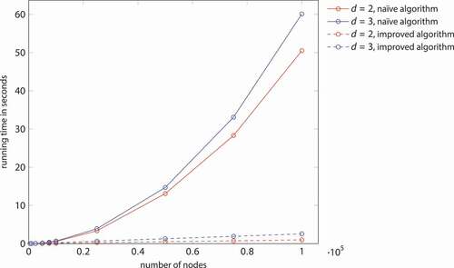
Figure 6. Running times of the improved algorithm for generating a Mocnik model ($\mathit{\rho }\mathbf{=}\mathbf{1}\mathbf{.6}$), both with and without parallel execution. (compare Table 3)

In both cases, the naïve and the improved algorithm, the computation of a Mocnik model is slower in higher dimensions. The reason is, however, a different one for these two algorithms. The running time of the naïve algorithm is, in principle, independent of the dimension and the arrangement of the nodes in space, because every node is compared to all others. Only the number of edges and thus the time needed to store the nodes and to evaluate distances increases. Running times depend thus only very little on the dimension, which is in contrast to the improved algorithm. The running time of the improved algorithm strongly depends on the number of grid cells in a hypercube, which, in turn, strongly increases by dimension. While the naïve algorithm is only about 10–20 per cent slower in three-dimensional space compared to a two-dimensional one, the improved algorithm is about 160 per cent slower (Figure 5 and Table 3).

The improved algorithm can be parallelized for making use of multiple cores. The loop iterating the grid cells consumes the largest part of the running time of Algorithm 2. Thereby, the only variable shared with write access is the set of edges. If edges can concurrently be added to the network, the parallelization of the largest part of the algorithm is straightforward. In the evaluated implementation, edges cannot be added concurrently. Instead, the edges are first collected in parallel and thereafter consecutively added to the network. When running on two cores instead of one, the improved algorithm is about 1.6 times as fast in two-dimensional space and 1.8 times in three-dimensional space (Figure 6 and Table 3).

5. Conclusion

Nearest-neighbour models inherit the notion of locality from the space they are embedded in. While this is an important feature when modelling spatial structure and spatial information, their generation can be time-consuming. The naïve algorithm determines the distance between every pair of nodes, resulting in quadratic running time. By using a spatial grid as an index for the nodes, the notion of locality can be exploited. In this article, we have introduced an improved algorithm, which is able to generate a Mocnik model in a very efficient way. It has been shown that, by choosing a suitable granularity of the spatial grid, a linear average-case time complexity can be achieved. As a result, it becomes possible to generate spatial networks with billions of nodes – the generation of a two-dimensional network with one million nodes takes less than 7 seconds on a laptop.

The Mocnik model and other nearest-neighbour models focus on inheriting properties of space, as is often needed for modelling spatial phenomena in an appropriate way. Nearest-neighbour models, however, do not reflect specific properties of real-world phenomena but rather make sense of space in a prototypical way. This is in contrast to many real-world examples. Public transport networks usually have a node degree strictly larger than one, the indegree and the outdegree coincide for most nodes, and the network has only very few connected components. In a road network, the node degree is usually limited by five. Communication networks are shaped by geographical space, by the way cities are organized, by structural elements within companies and organizations, etc. Time and temporal evolution are other important characteristics of many networks. Future research might address this issue by adapting nearest-neighbour models such that they reflect further properties of real-world phenomena. This way, the models will take further characteristics into consideration, which helps to improve the modelling quality and improves our understanding of such networks.

Big geospatial data challenges our conceptualizations, our algorithms, and our infrastructure, because the complexity, size, and heterogeneity of such data far exceed currently tractable limits. Structural views are suitable means to address such issues because they allow for abstraction. The effective generation of a Mocnik model at a large scale renders possible to examine how algorithms perform on prototypical spatial networks. For instance, an algorithm might perform well on small-world and much worse on spatial networks, or vice versa. Knowledge about the impact spatial structure has on networks can lead to insights about how to improve algorithms with respect to average-case time complexity and thus about how to become more efficient in real-world scenarios with spatial characteristics. When adapting an algorithm to the spatial structure of a network or some other data structure, computations can often be restricted to local neighbourhoods. That is, one can try to use the same approach that has already been successfully applied to the Mocnik model in this article. Also, additional ways of utilizing the notion of locality are worth to consider. The resulting algorithms might, in turn, be evaluated by applying them to a Mocnik model, or some other nearest-neighbour model.

Disclosure statement

The author reported no potential conflict of interest.

Data availability statement

The algorithm has been implemented as part of NetworKit (Staudt et al. 2016), an open-source toolkit for large-scale network analysis. It is available on https://networkit.github.io.

Notes

1. NetworKit is available at https://networkit.github.io.

Appendix to the article ‘An improved algorithm for dynamic nearest-neighbour models’ by Franz-Benjamin Mocnik

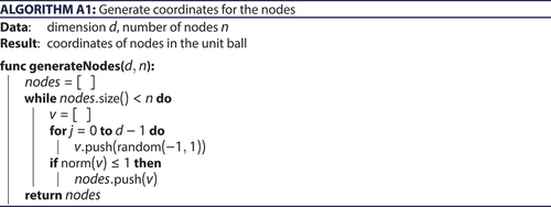
Appendix A. Generating randomly distributed nodes in the unit ball

Algorithm A1 generates coordinates for the nodes of a Mocnik model. In a first step, coordinates randomly placed within the hypercube of side length 2 and centred at the origin are created. In a second step, it is checked whether the coordinates are within the unit ball. If they are, the coordinates are kept; otherwise they are discarded. The algorithm repeats until $n$ nodes are found.

Table D1. Running times of the naïve and the improved algorithm, depending on the dimension of the embedding space. The running times refer the generation of a Mocnik model with 10,000 nodes and parameter $\rho =1.6$. All times are given in seconds.

Dimension	Naïve	Improved	Improved parallel
1	5.13·10^−1	4.15·10^−2	2.55·10^−2
2	5.28·10^−1	9.47·10^−2	5.56·10^−2
3	6.13·10^−1	2.50·10^−1	1.37·10^−1
4	7.04·10^−1	6.70·10^−1	3.62·10^−1
5	8.61·10^−1	1.76·10^0	9.90·10^−1
6	1.08·10^0	3.50·10^0	1.87·10^0
7	1.30·10^0	7.64·10^0	3.89·10^0
8	1.55·10^0	4.43·10^0	2.57·10^0
9	2.30·10^0	7.80·10^0	4.71·10^0
10	3.98·10^0	1.48·10^0	8.77·10^0

Table D2. Running times of the naïve and the improved algorithm, depending on the parameter $\mathit{\rho }$. The running times refer the generation of a Mocnik model with 10,000 nodes. All times are given in seconds.

	d = 2			d = 3
$\mathit{\rho }$	Naïve	Improved	Improved parallel	Naïve	Improved	Improved parallel
1.1	5.47·10^−1	1.14·10^−1	5.92·10^−2	6.15·10^−1	2.61·10^−1	1.35·10^−1
1.3	5.39·10^−1	9.88·10^−2	5.41·10^−2	6.26·10^−1	2.49·10^−1	1.39·10^−1
1.5	5.35·10^−1	9.95·10^−2	5.54·10^−2	6.45·10^−1	2.44·10^−1	1.39·10^−1
1.7	5.78·10^−1	9.62·10^−2	5.91·10^−2	6.73·10^−1	2.60·10^−1	1.43·10^−1
1.9	5.41·10^−1	1.05·10^−1	5.90·10^−2	6.49·10^−1	2.64·10^−1	1.50·10^−1
2.1	5.60·10^−1	9.95·10^−2	5.87·10^−2	6.46·10^−1	2.76·10^−1	1.52·10^−1
2.3	5.69·10^−1	1.01·10^−1	5.92·10^−2	6.95·10^−1	2.87·10^−1	1.62·10^−1
2.5	5.64·10^−1	1.03·10^−1	6.14·10^−2	6.69·10^−1	3.19·10^−1	1.77·10^−1
2.7	5.52·10^−1	1.03·10^−1	6.12·10^−2	6.57·10^−1	3.15·10^−1	1.79·10^−1
2.9	5.47·10^−1	1.09·10^−1	6.36·10^−2	6.49·10^−1	3.65·10^−1	2.04·10^−1
3.1	5.49·10^−1	1.09·10^−1	6.75·10^−2	6.46·10^−1	3.69·10^−1	2.08·10^−1
3.3	5.55·10^−1	1.12·10^−1	6.76·10^−2	6.44·10^−1	3.70·10^−1	2.12·10^−1
3.5	5.59·10^−1	1.14·10^−1	6.83·10^−2	6.78·10^−1	4.51·10^−1	2.59·10^−1
3.7	5.62·10^−1	1.16·10^−1	7.25·10^−2	6.79·10^−1	4.50·10^−1	2.58·10^−1
3.9	5.65·10^−1	1.19·10^−1	7.36·10^−2	6.69·10^−1	4.55·10^−1	2.64·10^−1
4.1	5.63·10^−1	1.23·10^−1	7.50·10^−2	6.65·10^−1	4.65·10^−1	2.69·10^−1
4.3	5.64·10^−1	1.32·10^−1	7.85·10^−2	6.64·10^−1	6.30·10^−1	3.51·10^−1
4.5	5.52·10^−1	1.35·10^−1	8.09·10^−2	6.65·10^−1	6.41·10^−1	3.58·10^−1
4.7	5.60·10^−1	1.35·10^−1	8.26·10^−2	6.83·10^−1	6.38·10^−1	3.66·10^−1
4.9	5.75·10^−1	1.39·10^−1	8.74·10^−2	6.97·10^−1	6.58·10^−1	3.63·10^−1
5.1	5.55·10^−1	1.48·10^−1	9.10·10^−2	7.14·10^−1	6.57·10^−1	3.67·10^−1
5.3	5.90·10^−1	1.48·10^−1	9.02·10^−2	6.86·10^−1	6.73·10^−1	3.76·10^−1
5.5	5.88·10^−1	1.54·10^−1	9.49·10^−2	7.13·10^−1	6.66·10^−1	3.80·10^−1
5.7	5.78·10^−1	1.55·10^−1	9.52·10^−2	7.36·10^−1	9.51·10^−1	5.81·10^−1
5.9	5.74·10^−1	1.66·10^−1	1.01·10^−1	7.16·10^−1	9.50·10^−1	5.77·10^−1
6.1	6.07·10^−1	1.66·10^−1	1.03·10^−1	7.38·10^−1	9.86·10^−1	5.85·10^−1
6.3	5.69·10^−1	1.68·10^−1	1.03·10^−1	7.67·10^−1	9.75·10^−1	6.06·10^−1
6.5	5.86·10^−1	1.79·10^−1	1.09·10^−1	7.53·10^−1	9.78·10^−1	6.12·10^−1
6.7	5.84·10^−1	1.87·10^−1	1.11·10^−1	7.63·10^−1	9.84·10^−1	6.23·10^−1
6.9	5.81·10^−1	1.79·10^−1	1.13·10^−1	7.69·10^−1	1.01·10^0	6.35·10^−1
7.1	5.80·10^−1	1.95·10^−1	1.19·10^−1	7.93·10^−1	1.00·10^0	6.31·10^−1
7.3	5.80·10^−1	2.03·10^−1	1.21·10^−1	7.88·10^−1	1.03·10^0	6.55·10^−1
7.5	6.26·10^−1	1.96·10^−1	1.20·10^−1	7.93·10^−1	1.04·10^0	6.64·10^−1
7.7	5.95·10^−1	2.02·10^−1	1.22·10^−1	7.93·10^−1	1.06·10^0	6.74·10^−1
7.9	5.90·10^−1	2.17·10^−1	1.32·10^−1	8.11·10^−1	1.08·10^0	6.73·10^−1
8.1	5.89·10^−1	2.28·10^−1	1.32·10^−1	8.26·10^−1	1.12·10^0	6.99·10^−1
8.3	6.01·10^−1	2.20·10^−1	1.37·10^−1	8.44·10^−1	1.13·10^0	7.09·10^−1
8.5	6.05·10^−1	2.24·10^−1	1.35·10^−1	8.61·10^−1	1.14·10^0	7.43·10^−1
8.7	6.00·10^−1	2.25·10^−1	1.39·10^−1	8.52·10^−1	1.54·10^0	9.12·10^−1
8.9	6.05·10^−1	2.57·10^−1	1.56·10^−1	8.91·10^−1	1.6·10^0	9.19·10^−1
9.1	6.10·10^−1	2.58·10^−1	1.60·10^−1	9.07·10^−1	1.58·10^0	9.33·10^−1
9.3	6.06·10^−1	2.60·10^−1	1.55·10^−1	9.18·10^−1	1.59·10^0	9.52·10^−1
9.5	6.00·10^−1	2.59·10^−1	1.55·10^−1	9.43·10^−1	1.62·10^0	9.39·10^−1
9.7	6.02·10^−1	2.63·10^−1	1.61·10^−1	9.39·10^−1	1.65·10^0	1.00·10^0
9.9	6.03·10^−1	2.67·10^−1	1.62·10^−1	9.47·10^−1	1.69·10^0	1.00·10^0
10.1	6.07·10^−1	2.69·10^−1	1.62·10^−1	9.84·10^−1	1.69·10^0	1.01·10^0

Algorithm A1 ideally computes $n$ times the coordinates of a $d$-dimensional vector, i.e., it ideally would be of complexity O(d · n). However, some coordinates need to be discarded, which is why the algorithm has to compute more than n coordinates. The volume of the $d$-dimensional unit ball is ${\pi }^{d/2}/\mathrm{\Gamma }(d/2+1)$, whereas the volume of the hypercube of side length 2 is 2${ }^d$. On average, only each $(2/\sqrt{\pi }{)}^d\cdot \mathrm{\Gamma }(d/2+1)$-th vector will thus be contained in the unit ball. The overall complexity of Algorithm A1 is thus $O(d\cdot (2/\sqrt{\pi }{)}^d\cdot \mathrm{\Gamma }(d/2+1)\cdot n)$ on average. For a fixed dimension, the complexity is thus linear.

Appendix B. Indexing the nodes in a spatial grid

The improved algorithm stores the nodes in a spatial grid to efficiently find nodes in the same vicinity. In this section, we introduce three straightforward algorithms to store and retrieve identifiers (IDs) in such a spatial grid.

Algorithms B1a and B1b convert between integer coordinates of a grid cell and their corresponding IDs. Algorithm B1a converts integer coordinates of a grid cell, i.e., a $d$-dimensional vector of integers, to an ID, i.e., only one integer value. Such an ID can be used to efficiently represent grid cells in the memory. In particular, the IDs of the grid cells can be used as an index of a vector. By storing the corresponding collection of nodes in each component of the vector, the nodes can easily be indexed by their enclosing grid cells. Algorithm B1b converts back an ID of a node to integer coordinates. Both Algorithms B1a and B1b have complexity $O(d)$, because they execute the same computations for every dimension. For a fixed dimension, these algorithms are thus of complexity O(1).

Algorithm B2 determines, for given d-dimensional coordinates of a node, the grid cell of the spatial grid that contains the node. By and large, the algorithm only rounds the coordinates, resulting in the integer coordinates of the grid cell. These integer coordinates are then converted to the ID of corresponding the cell by utilizing Algorithm B1a. As Algorithm B2 considers each dimension and applies Algorithm B1a thereafter, it is of complexity O(d). For a fixed dimension, the algorithm is thus of complexity O(1).

Appendix C. Volume and surface of a hypercube inside the spatial grid

The spatial grid discussed in the previous section can serve as a spatial index for nodes. In this section, we provide algorithms to determine neighbourhoods in the spatial grid, i.e., grid cells adjacent to a given one. These algorithms render possible to query, for a given node, all neighbouring nodes within a certain distance in a very efficient way.

Figure D1. Running times of the naïve and the improved algorithm, depending on the dimension of the embedding space. The running times refer the generation of a Mocnik model with 10,000 nodes and parameter ρ = 1.6. (compare Table D1)

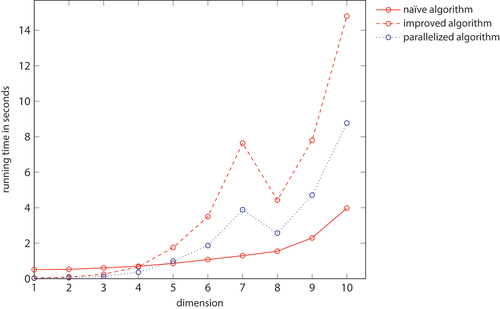
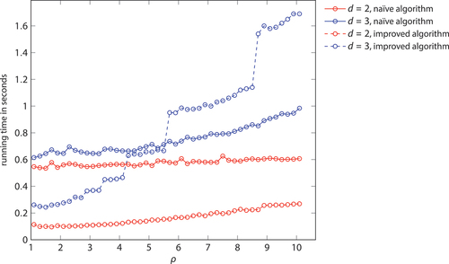
Figure D2. Running times of the naïve and the improved algorithm, depending on the parameter $\mathit{\rho }$. The running times refer the generation of a Mocnik model with 10,000 nodes. (compare Table D2)

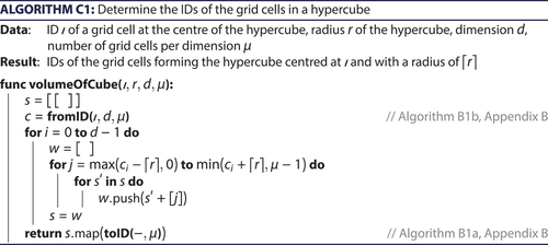
Given a centre grid cell, Algorithm C1 determines all grid cells that are at most r steps away in each direction, i.e., a hypercube of grid cells. In a first step, the ID of the provided centre grid cell is converted to a d-dimensional vector of integers, which represents its location inside the grid. Subsequently, the algorithm determines the grid cells that form the hypercube. For this purpose, a collection is initialized, which ultimately contains the integer coordinates of these grid cells. Starting with an empty vector in the collection, vector components are successively added to the vectors of this collection, one for each dimension of the space. Thereby, each vector of the collection is in each step replaced by several extended vectors, which have one more component. This component ranges from –r to r (relatively to the centre node), resulting in 2r + 1 vectors. In subsequent steps, additional components are added, thereby multiplying the number of vectors contained in the collection – each combination of values needs to be considered. Finally, the resulting integer coordinates are converted into IDs.

Algorithm C2 is very similar to Algorithm C1 but returns only the ‘outer’ grid cells of the hypercube. This is in so far useful as an algorithm looking for nodes in the vicinity of a given centre node can increase the search radius successively until a sufficient number of nodes has been found. More and more grid cells can be considered without the need to consider a grid cell several times, as would be the case when using hypercubes of increasing edge length. The algorithm to find the ‘outer’ grid cells first checks whether r vanishes. In this case, the grid cell itself is returned. Otherwise, the integer coordinates of the grid cells are generated. For every component, all values between –r and r (relatively to the corresponding component of the centre node) are combined, as is the case in Algorithm C1. One dimension is though omitted in this iteration, and only the two extreme values –r and r rather than the full range are inserted. When generating the grid cell vectors this way, some vectors occur several times. To minimize duplicate values, the first loop does not need to consider the extreme values because they are already considered when i vanishes. In addition, remaining duplicates are removed in the last step.

Algorithm C1 is of complexity O(d·(2r)^d), because each vector consists of d components and the number of grid cells contained in the hypercube is (2r + 1)^d. The surface area of the hypercube is 2d · (2r + 1)^d–1. Accordingly, Algorithm C2 has complexity O(d² · (2r)^d–1). For a fixed dimension, the algorithms have complexity O(r^d) respective O(r^d–1).

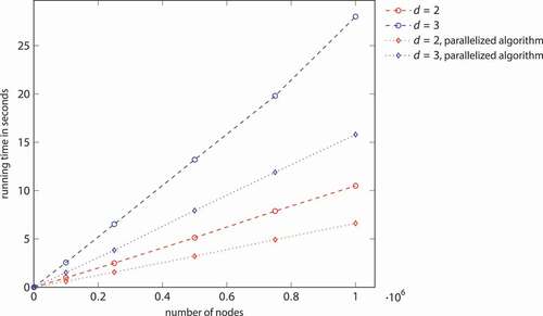
Appendix D. Empirical running time evaluation, Part II

The running times of the naïve and the improved algorithms depend on the number of nodes, the dimension of the embedding space, and the parameter ρ. The influence of the number of nodes on running times has empirically been examined in the article (Table 3 and Figures 5 and 6). In this section, we provide corresponding tables and figures for the influence of the embedding space (Table D1 and Figure D1) and for the parameter ρ (Table D2 and Figure D2).

The way running times depend on the dimension of the embedding space and the parameter ρ is, by and large, as expected. The larger the dimension and the larger the parameter ρ, the less efficient is the improved algorithm compared to the naïve one. This is because the network becomes more and more complete in this case, and the advantage of an index becomes less prominent. However, it needs to be noted that such cases of larger dimension and larger parameter ρ are not very common, as they lead to very dense and ultimately to almost complete networks. For a larger number of nodes, this effect would be less prominent.

The interpretation of the displayed running times at larger dimensions and larger parameter ρ is not straight forward because the resulting network is near to complete. There are different processes involved that sum up to the overall running time experienced in the implementation, in particular, the computation itself, memory management, communication between the C backend and the Python frontend, building the network representation in Python, outputting the network representation, etc. These influences on the running times superimpose, which is why they do not monotonously depend on the dimension, and why they show discontinuities with respect to the parameter ρ.

References

- Albert, R., Jeong, H., and Barabási, A.L., 1999. Diameter of the World-Wide Web. Nature, 401 (6749), 130–131. doi:10.1038/43601
- Aldous, D.J. and Ganesan, K., 2013. True scale-invariant random spatial networks. Proceedings of the National Academy of Sciences of the United States of America, 110 (22), 8782–8785. doi:10.1073/pnas.1304329110
- Aldous, D.J. and Shun, J., 2010. Connected spatial networks over random points and a route-length statistic. Statistical Science, 25 (3), 275–288. doi:10.1214/10-STS335
- Allen, J.F., 1983. Maintaining knowledge about temporal intervals. Communications of the ACM, 26 (11), 832–843. doi:10.1145/182.358434
- Anselin, L., 1995. Local indicators of spatial association – LISA. Geographical Analysis, 27 (2), 93–115. doi:10.1111/j.1538-4632.1995.tb00338.x
- Backstrom, L., et al., 2012. Four degrees of separation. Proceedings of the 4th Annual ACM Web Science Conference (WebSci), Evanston, IL, 33–42.
- Barabási, A.L., et al., 2002. Evolution of the social network of scientific collaborations. Physica A, 311 (3–4), 590–614. doi:10.1016/S0378-4371(02)00736-7
- Barabási, A.L. and Albert, R., 1999. Emergence of scaling in random networks. Science, 286 (5439), 509–512. doi:10.1126/science.286.5439.509
- Barabási, A.L., Albert, R., and Jeon, H., 2000. Scale-free characteristics of random networks: the topology of the World-Wide Web. Physica A, 281 (1–4), 69–77. doi:10.1016/S0378-4371(00)00018-2
- Barabási, A.L. and Bonabeau, E., 2003. Scale-free networks. Scientific American, 288 (5), 50–59. doi:10.1038/scientificamerican0503-60
- Barnes, T.J., 2004. A paper related to everything but more related to local things. Annals of the Association of American Geographers, 94 (2), 278–283. doi:10.1111/j.1467-8306.2004.09402004.x
- Barthélemy, M., 2011. Spatial networks. Physics Reports, 499 (1–3), 1–101. doi:10.1016/j.physrep.2010.11.002
- Baum, J.A.C., Shipilov, A.V., and Rowley, T.J., 2003. Where do small worlds come from? Industrial and Corporate Change, 12 (4), 697–725. doi:10.1093/icc/12.4.697
- Beckmann, N., et al., 1990. The R*-tree: an efficient and robust access method for points and rectangles. Proceedings of the 16th ACM International Conference on Management of Data (SIGMOD), Atlantic City, NJ, 322–331.
- Bentley, J.L., 1975a. Multidimensional binary search trees used for associative searching. Communications of the ACM, 18 (9), 509–517. doi:10.1145/361002.361007
- Bentley, J.L., 1975b. A survey of techniques for fixed radius near neighbor searching. Stanford Linear Accelerator Center, Menlo Park, CA: Stanford University. SLAC-186, STAN-CS-75-513.
- Bentley, J.L., Stanat, D.F., and Williams, E.H., Jr., 1977. The complexity of finding fixed-radius near neighbors. Information Processing Letters, 6 (6), 209–212. doi:10.1016/0020-0190(77)90070-9
- Bullmore, E. and Sporns, O., 2009. Complex brain networks: graph theoretical analysis of structural and functional systems. Nature Reviews Neuroscience, 10 (3), 186–198. doi:10.1038/nrn2575
- Burke, J., et al., 2006. Participatory sensing. Proceedings of the 1st Workshop on World-Sensor-Web: Mobile Device Centric Sensory Networks and Applications (WSW). Boulder, CO.
- Cheung, K.L. and Fu, A.W.-c., 1998. Enhanced nearest neighbour search on the R-tree. ACM SIGMOD Record, 27 (3), 16–21. doi:10.1145/290593.290596
- DeLyser, D. and Sui, D.Z., 2012. Crossing the qualitative-quantitative divide II: inventive approaches to big data, mobile methods, and rhythmanalysis. Progress in Human Geography, 37 (2), 293–305. doi:10.1177/0309132512444063
- Egenhofer, M.J., 1991. Reasoning about binary topological relations. Proceedings of the 2nd International Symposium on Advances in Spatial Databases (SSD), Zurich, Switzerland, 143–160.
- Figueroa, K. and Paredes, R., 2009. Approximate direct and reverse nearest neighbor queries, and the k-nearest neighbor graph. Proceedings of the 2nd International Workshop on Similarity Search and Applications (SISAP), Prague, Czech Republic, 91–98. doi:10.1016/j.antiviral.2009.07.022
- Finkel, R.A. and Bentley, J.L., 1974. Quad trees. A data structure for retrieval on composite keys. Acta Informatica, 4 (1), 1–9. doi:10.1007/BF00288933
- Fogliaroni, P., 2013. Qualitative spatial configuration queries. Towards next generation access methods for GIS. Amsterdam: IOS.
- Friedman, J.H., Bentley, J.L., and Finkel, R.A., 1977. An algorithm for finding best matches in logarith- mic expected time. ACM Transactions on Mathematical Software, 3 (3), 209–226. doi:10.1145/355744.355745
- Gao, J., et al., 2015. Selective hashing: closing the gap between radius search and k-NN search. Proceedings of the 21st ACM SIGKDD International Conference on Knowledge Discovery and Data Mining, Sydney, Australia, 349–358.
- Gilbert, E.N., 1959. Random graphs. Annals of Mathematical Statistics, 30 (4), 1141–1144. doi:10.1214/aoms/1177706098
- Glückler, J., 2007. Economic geography and the evolution of networks. Journal of Economic Geography, 7 (5), 619–634. doi:10.1093/jeg/lbm023
- Goodchild, M.F., 2004. The validity and usefulness of laws in geographic information science and geography. Annals of the Association of American Geographers, 94 (2), 300–303. doi:10.1111/j.1467-8306.2004.09402008.x
- Goodchild, M.F., 2007. Citizens as sensors: the world of volunteered geography. GeoJournal, 69 (4), 211–221. doi:10.1007/s10708-007-9111-y
- Guttman, A., 1984. R-trees: a dynamic index structure for spatial searching. Proceedings of the 10th ACM International Conference on Management of Data (SIGMOD), Boston, MA, 47–57.
- Haggett, P. and Chorley, R.J., 1969. Network analysis in geography. London: Edward Arnold.
- Harvey, F.J., 2013. A new age of discovery: the post-GIS era. Proceedings of the GI_Forum, Salzburg, Austria, 272–281.
- Hecht, B. and Moxley, E., 2009. Terabytes of Tobler: evaluating the first law in a massive, domain- neutral representation of world knowledge. Proceedings of the 9th International Conference on spatial information theory (COSIT), Aber Wrac'h, France, 88–105.
- Hjaltason, G.R. and Samet, H., 1995. Ranking in spatial databases. Proceedings of the 4th Symposium on Spatial Databases, Portland, ME, 83–95. doi:10.1177/014860719501900183
- Holland, P.W. and Leinhardt, S., 1981. An exponential family of probability distributions for directed graphs. Journal of the American Statistical Association, 76 (373), 33–50. doi:10.1080/01621459.1981.10477598
- Holme, P. and Saramäki, J., 2012. Temporal networks. Physics Reports, 519 (3), 97–125. doi:10.1016/j.physrep.2012.03.001
- Hunter, D.R., Goodreau, S.M., and Handcock, M.S., 2008. Goodness of fit of social network models. Journal of the American Statistical Association, 103 (481), 248–258. doi:10.1198/016214507000000446
- Huttenhower, C., et al., 2007. Nearest neighbor networks: clustering expression data based on gene neighborhoods. BMC Bioinformatics, 8 (1), 250. doi:10.1186/1471-2105-8-250
- Kalapala, V., et al., 2006. Scale invariance in road networks. Physical Review E, 73 (2), 026130. doi:10.1103/PhysRevE.73.026130
- Kamel, I. and Faloutsos, C., 1994. Hilbert R-tree: an improved R-tree using fractals. Proceedings of the 20th International Conference on Very Large Data Bases (VLDB), Santiago de Chile, Chile, 500–509.
- Knuth, D.E., 1973. The art of computer programming. Vol. 3. Reading, MA: Addison-Wesley.
- Kuratowski, C., 1930. Sur le problème des courbes gauches en topologie. Fundamenta Mathematicae, 15 (1), 271–283. doi:10.4064/fm-15-1-271-283
- Kurniawati, R., Jin, J.S., and Shepard, J.A., 1997. SS+ tree: an improved index structure for similarity searches in a high-dimensional feature space. Proceedings of the SPIE Electronic Imaging Conference, San José, CA, 110–120.
- Levin, L.A., 1986. Average case complete problems. SIAM Journal on Computing, 15 (1), 285–286. doi:10.1137/0215020
- Levinthal, C., 1966. Molecular model-building by computer. Scientific American, 214 (6), 42–52. doi:10.1038/scientificamerican0666-42
- Li, M., Westerholt, R., and Zipf, A., 2018. Do people communicate about their whereabouts? Investigating the relation between user-generated text messages and Foursquare check-in places. Geo-spatial Information Science, 21 (3), 159–172. doi:10.1080/10095020.2018.1498669
- Louf, R., Roth, C., and Barthélemy, M., 2014. Scaling in transportation networks. PLoS ONE, 9 (7), e102007. doi:10.1371/journal.pone.0102007
- MacLane, S., 1937. A combinatorial condition for planar graphs. Fundamenta Mathematicae, 28 (1), 22–31.
- Mattson, W. and Rice, B.M., 1999. Near-neighbor calculations using a modified cell-linked list method. Computer Physics Communications, 119 (2–3), 135–148. doi:10.1016/S0010-4655(98)00203-3
- Micó, M.L., Oncina, J., and Carrasco, R.C., 1996. A fast branch & bound nearest neighbour classifier in metric spaces. Pattern Recognition Letters, 17 (7), 731–739. doi:10.1016/0167-8655(96)00032-3
- Micó, M.L., Oncina, J., and Vidal, E., 1994. A new version of the nearest-neighbour approximating and eliminating search algorithm (AESA) with linear preprocessing time and memory requirements. Pattern Recognition Letters, 15 (1), 9–17. doi:10.1016/0167-8655(94)90095-7
- Miller, H.J., 2004. Tobler’s first law and spatial analysis. Annals of the Association of American Geographers, 94 (2), 284–289. doi:10.1111/j.1467-8306.2004.09402005.x
- Mocnik, F.-B., 2015a. Modelling spatial information. Proceedings of the 1st Vienna Young Scientists Symposium (VSS), Vienna, Austria, 46–47.
- Mocnik, F.-B., 2015b. A scale-invariant spatial graph model. Thesis (PhD). Vienna University of Technology.
- Mocnik, F.-B., 2018a. Dimension as an invariant of street networks. Proceedings of the 7th International Conference on Complex Networks and Their Applications, Cambridge, UK, 455–457.
- Mocnik, F.-B., 2018b. The polynomial volume law of complex networks in the context of local and global optimization. Scientific Reports, 8, 11274. doi:10.1038/s41598-018-29131-0
- Mocnik, F.-B., 2018c. Tradition as a spatiotemporal process – the case of Swedish folk music. Proceedings of the 21st AGILE Conference on Geographic Information Science. Lund, Sweden.
- Mocnik, F.-B. and Frank, A.U., 2015. Modelling spatial structures. Proceedings of the 12th Conference on Spatial Information Theory (COSIT), Santa Fe, NM, 44–64. http://doi.org/10.1007/978-3-319-23374-1_3
- Nelson, R.C. and Samet, H., 1987. A population analysis for hierarchical data structures. Proceedings of the 13th ACM International Conference on Management of Data (SIGMOD), San Francisco, CA, 270–277.
- Newman, M.E.J., 2001. The structure of scientific collaboration networks. Proceedings of the National Academy of Sciences of the United States of America, 98 (2), 404–409. doi:10.1073/pnas.98.2.404
- Onnela, J.P., et al., 2007. Analysis of a large-scale weighted network of one-to-one human communication. New Journal of Physics, 9 (6), 179. doi:10.1088/1367-2630/9/6/179
- Phillips, J.D., 2004. Doing justice to the law. Annals of the Association of American Geographers, 94 (2), 290–293. doi:10.1111/j.1467-8306.2004.09402006.x
- Roussopoulos, N., Kelley, S., and Vincent, F., 1995. Nearest neigbor queries. Proceedings of the 21st ACM International Conference on Management of Data (SIGMOD), San José, CA, 71–79. doi:10.1016/0306-4522(94)00460-m
- Roussopoulos, N. and Leifker, D., 1985. Direct spatial search on pictorial databases using packed R-trees. Proceedings of the 11st ACM International Conference on Management of Data (SIGMOD), Austin, TX, 17–31.
- Sala, A., et al., 2010. Measurement-calibrated graph models for social network experiments. Proceedings of the 19th International World Wide Web Conference (WWW), Raleigh, NC, 861–870.
- Smith, J.M., 2004. Unlawful relations and verbal inflation. Annals of the Association of American Geographers, 94 (2), 294–299. doi:10.1111/j.1467-8306.2004.09402007.x
- Sporns, O., Tonoi, G., and Kötter, R., 2005. The human connectome: a structural description of the human brain. PLoS Computational Biology, 1 (4), e42. doi:10.1371/journal.pcbi.0010042
- Sproull, R.F., 1991. Refinements to nearest-neighbor searching in k-dimensional trees. Algorithmica, 6 (1–6), 579–589. doi:10.1007/BF01759061
- Staudt, C., Sazonovs, A., and Meyerhenke, H., 2016. NetworKit: a tool suite for large-scale complex network analysis. Network Science, 4 (4), 508–530. doi:10.1017/nws.2016.20
- Stefanidis, A., Crooks, A., and Radzikowski, J., 2013. Harvesting ambient geospatial information from social media feeds. GeoJournal, 78 (2), 319–338. doi:10.1007/s10708-011-9438-2
- Sui, D.Z., 2004. Tobler’s first law of geography: a big idea for a small world? Annals of the Association of American Geographers, 94 (2), 269–277. doi:10.1111/j.1467-8306.2004.09402003.x
- Tobler, W.R., 1970. A computer movie simulating urban growth in the Detroit region. Economic Geography, 46, 234–240. doi:10.2307/143141
- Tobler, W.R., 1999. Linear pycnophylactic reallocation comment on a paper by D. Martin. International Journal of Geographical Information Science, 13 (1), 85–90. doi:10.1080/136588199241472
- Tobler, W.R., 2004. On the first law of geography: a reply. Annals of the Association of American Geographers, 94 (2), 304–310. doi:10.1111/j.1467-8306.2004.09402009.x
- Tokoro, K., Yamaguchi, K., and Masuda, S., 2006. Improvements of TLAESA nearest neighbour search algorithm and extension to approximation search. Proceedings of the 29th Australasian Computer Science Conference (ACSC), Hobart, Australia, 77–83.
- van den Heuvel, M.P., et al., 2012. High-cost, high-capacity backbone for global brain communication. Proceedings of the National Academy of Sciences of the United States of America, 109 (28), 11372–11377. doi:10.1073/pnas.1203593109
- Vidal, E., 1994. New formulation and improvements of the nearest-neighbour approximating and elimi- nating search algorithm (AESA). Pattern Recognition Letters, 15 (1), 1–7. doi:10.1016/0167-8655(94)90094-9
- Wagner, K., 1937. Über eine Eigenschaft der ebenen Komplexe. Mathematische Annalen, 114 (1), 570–590. doi:10.1007/BF01594196
- Watts, D.J. and Strogatz, S.H., 1998. Collective dynamics of small-world networks. Nature, 393 (6684), 440–442. doi:10.1038/30918
- Waxman, B.M., 1988. Routing of multipoint connections. IEEE Journal on Selected Areas in Communications, 6 (9), 1617–1622. doi:10.1109/49.12889
- Weiss, S.F., 1980. A probabilistic algorithm for nearest neighbour searching. Proceedings of the 3rd Annual ACM Conference on Research and Development in Information Retrieval, Cambridge, UK, 325–333.
- Westerholt, R., et al., 2016. Abundant topological outliers in social media data and their effect on spatial analysis. PLOS ONE, 11 (9), e0162360. doi:10.1371/journal.pone.0162360
- Westlund, H., 2013. A brief history of time, space, and growth: Waldow Tobler’s first law of geography revisited. The Annals of Regional Science, 51 (3), 917–924. doi:10.1007/s00168-013-0571-3
- White, D.A. and Jain, R., 1996. Similarity indexing with the SS-tree. Proceedings of the 12th International Conference on Data Engineering (ICDE), New Orleans, LA, 516–523.
- Whitney, H., 1931. Non-separable and planar graphs. Proceedings of the National Academy of Sciences of the United States of America, 17 (2), 125–127. doi:10.1073/pnas.17.2.125
- Xia, C., Hsu, W., and Lee, M.L., 2005. ERkNN: efficient reverse k-nearest neighbors retrieval with local kNN-distance estimation. Proceedings of the 14th ACM International Conference on Information and Knowledge Management (CIKM), Bremen, Germany, 533–540.
- Yook, S.H., Jeong, H., and Barabási, A.L., 2002. Modeling the internet’s large-scale topology. Proceedings of the National Academy of Sciences of the United States of America, 99 (21), 13382–13386. doi:10.1073/pnas.172501399
- Zhong, X.F., et al., 2017. An improved k-NN classification with dynamic k. Proceedings of the 9th International Conference on Machine Learning and Computing (ICMLC). Singapore, 211–216.