Predicting land use and land cover change dynamics in the eThekwini Municipality: a machine learning approach with Landsat imagery

ABSTRACT

Monitoring and providing accurate land use and land cover (LULC) change information is vital for sustainable environmental planning. This study used Landsat imagery from 2002 to 2022 to create updated LULC change maps for the eThekwini Municipality. Random Forest (RF), Support Vector Machine (SVM), and Extreme Gradient Boosting (XGBoost) were used to conduct these LULC classifications, with XGBoost achieving the highest accuracy (80.57%). The generated maps revealed a significant decrease in cropland and an increase in impervious surfaces. As such, this research established a framework for continuous LULC mapping and highlighted Landsat 9’s potential in LULC classifications.

KEYWORDS:

• Land cover
• land use
• remote sensing
• machine learning
• Landsat

1. Introduction

The complex environmental, social, economic, and political matrix is the primary driver of a territory’s spatial arrangement (Trujillo-Jiménez et al. 2022). This matrix has also accelerated the natural Earth’s surface changes through increased resource consumption to compensate for increased human populations and accelerated economic development (Kafy et al. 2021, Digra et al. 2022). Land use and land cover (LULC) maps serve as excellent depictions of this matrix (Trujillo-Jiménez et al. 2022), primarily because producing up-to-date and accurate LULC change information provides an understanding of human-environment relationships and the adverse impacts of global change (Chakraborty et al. 2016, Nasiri et al. 2022). Moreover, this updated information also provides crucial insights for implementing sustainable land management practices, conserving natural resources, and enhancing resilience to climate-related hazards (Effiong et al. 2024). Therefore, LULC change information, especially at the regional scale, aids decision-makers in mitigating the persisting challenges of global change that results from LULC change through appropriate environmental management policies and strategies (Ai et al. 2020, Tadese et al. 2020). Thus, LULC maps are the key to sustainable environmental planning and development (González-González et al. 2022). This primarily pertains to impoverished rural regions, some of which are key areas for ecological and biodiversity significance (Musetsho et al. 2021).

The eThekwini Municipality has attempted to protect and manage its biodiversity and ecological hotspots that supply ecosystem services crucial for human well-being by establishing the Durban Metropolitan Open Space System (DMOSS) (Boon et al. 2016). This was due to the increased degradation and loss of the vegetated landscapes within the municipality (Zungu et al. 2020). However, the eThekwini Municipality is still susceptible to adverse environmental consequences due to the change driven by the municipality’s attempts to move past the apartheid’s discriminative spatial planning (Sutherland et al. 2014). Additionally, there is a lack of comprehensive knowledge and understanding regarding the rate of LULC change within the municipality and its ramifications for ecosystems and ecosystem services. Therefore, by providing updated LULC change maps, the eThekwini Municipality can implement appropriate environmental or spatial management policies and strategies. These maps will also inform an update to the DMOSS layer, which was last updated in 2018.

Generating LULC change maps previously relied on in situ monitoring techniques (Buchhorn et al. 2020). However, the prominence of remote sensing over the past decades, and the improved accessibility and development of various methods for extracting remotely sensed data has seen more LULC mapping studies utilizing remote sensing (Amini et al. 2022). Remote sensing presents the ability to effectively capture LULC change information (Nkundabose 2021) by making it possible to integrate spectral-temporal metrics and a diverse set of features to capture changes in various LULC classes (Liang et al. 2022). Most studies have utilized medium-resolution sensors such as Landsat (30 meters – m) and Sentinel 2 (10 m) given that these sensors can detect most human-nature interactions (Chen et al. 2015). These sensors also provide a short revisit time and vast spectral configurations (Nasiri et al. 2022). Hence, this research utilized imagery from Landsat 7 (Enhanced Thematic Mapper – ETM+), Landsat 8 (Operational Land Imager 1 - OLI 1), and Landsat 9 (Operational Land Imager 2 - OLI 2) with a spatial resolution of 30 m to analyze the changes in LULC within the eThekwini Municipality. The selection of these three sensors is also based on the consistency of the Landsat data record across the entire Landsat sensor series (Roy et al. 2016).

The utilization of remote sensing in mapping LULC change has attracted the application of machine and deep learning approaches. These approaches are applied to reduce spectral and spatial limitations associated with medium and low-resolution LULC classifications, which should result in more precise LULC maps (Talukdar et al. 2020). Some of the most popular algorithms in LULC change classification include Artificial Neural Networks (ANN), random forests (RF), Cellular Automata (CA), support vector machines (SVM), Markov Chain, and extreme gradient boosting (XGBoost) (Abdi 2020, Kafy et al. 2021). However, RF and SVM tend to produce more accurate LULC maps compared to the algorithms aforementioned (Abdi 2020, Talukdar et al. 2020, Ali et al. 2022).

Therefore, this research investigated the effectiveness of three machine learning algorithms, specifically, SVM, RF, and XGBoost in mapping changes in LULC. However, it should be noted that remote sensing based LULC change classifications can be limited by the requirement to access and store large remote sensing data and high computational costs. Platforms, such as the Google Earth Engine (GEE), which is cloud-based, have overcome these limitations (Tassi and Vizzari 2020). GEE allows scientists and independent researchers to access large data banks for change detection freely and quantify resources on the Earth’s surface (Mutanga and Kumar 2019). Therefore, Landsat data were obtained and processed in GEE.

Overall, the objective of the study was to map LULC change from 2002 to 2022 within the eThekwini Municipality using the three most recent Landsat sensors and machine learning algorithms. This will aid in assessing the present rate of LULC change and identifying the factors responsible for these changes. The absence of comprehensive knowledge on the rate of LULC change and the lack of understanding of the consequences of LULC change for ecosystems and ecosystem services within the eThekwini Municipality highlight the critical need for updated LULC change maps to inform decision-making and policy development. This research addresses these gaps by providing enhanced accuracy and efficiency in LULC mapping by employing machine learning algorithms. Such advanced methodologies bring significant advancement to the fields of remote sensing and spatial science, enabling more precise monitoring and analysis of land use and cover dynamics. Furthermore, including Landsat 9 imagery expands the temporal scope of the study. It also enhances the accuracy of LULC change detection, emphasizing its importance in improving the understanding of landscape dynamics over time. Consequently, the generated maps will not only facilitate the identification of areas for vegetation restoration within the eThekwini Municipality but also contribute to developing appropriate environmental or spatial management policies and strategies. Thus, the study’s findings will provide policymakers with invaluable insights to make decisions that are well-aligned with practical realities and sustainability goals.

2. Materials and methods

2.1. Study area

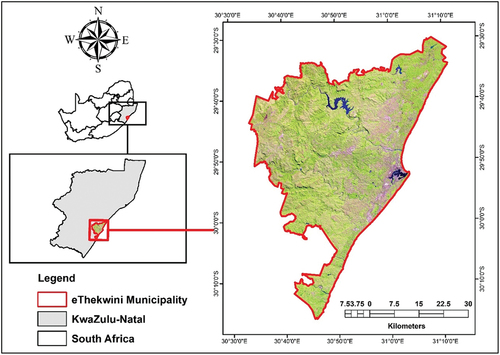
The eThekwini Municipality, established in 2000, is located in the South African province of KwaZulu-Natal (Figure 1), along the Indian Ocean’s eastern coast (Musvoto et al. 2016, Shivambu et al. 2020). The municipality serves as a pivotal economic hub in South Africa, largely due to its renowned port which is recognized as the busiest port, on the African continent (Zungu et al. 2020). The municipality is formed by 103 wards with an approximate population of 3.5 million, which grows by one percent annually (Zungu et al. 2019). Moreover, its mainland predominantly comprises urbanized zones, constituting the city of Durban, which is surrounded by peri-urban residential areas and informal settlements, along with rural communities (Hellberg 2014). With the population and rural-urban migration increasing and more residential spaces being required, the municipality established the DMOSS, a network of areas reserved for conserving native fauna and flora (Khumalo and Sibanda 2019, Zungu et al. 2019). DMOSS also aimed to limit the conversion of native vegetation for anthropogenic purposes, which include agriculture, residential areas, and roads. As of 2019, 53% of native vegetation had already been converted for human benefit (Zungu et al. 2020).

Figure 1. The eThekwini Municipality’s location in KwaZulu-Natal, South Africa.

2.2. Data acquisition and pre-processing

2.2.1. Reference data

The 2017 Finer Resolution Observation and Monitoring-Global Land Cover-Segmentation at 10 m (FROM – GLCS10) was used as a reference. FROM – GLCS10 offers a fundamental land cover scheme that incorporates continuous field layers for all primary land cover classes. These classes provide proportionate estimates of vegetation/ground cover for the respective land cover types. Classes in land-cover products generally utilize a hierarchical structure and, thus, this is also the case in FROM – GLCS10 (Zhu et al. 2021). The classes in FROM – GLCS10 found within the eThekwini Municipality are presented in Table 1. The LULC class descriptions are derived from the descriptions provided by Wei et al. (2020) and Buthelezi et al. (2024).

Table 1. From – GLCS10 land cover classes (Wei et al. 2020, Buthelezi et al. 2024).

Name	Description	Code
Cropland	Land under cultivation showing discernible patterns on satellite imagery.	1
Forest	Areas designated for commercial plantations, orchards, and native tree species.	2
Grassland	Areas that comprise open landscapes dominated by various species of grasses.	3
Shrubland	Land characterised by low-lying vegetation dominated by shrubs.	4
Wetland	Areas characterised by saturated or seasonally saturated soils	5
Water	Areas characterised by the presence of rivers, lakes, ponds, and reservoirs.	6
Tundra	Treeless landscapes in cold regions with vegetation adapted to harsh conditions, including mosses and lichens.	7
Impervious surface	Encompasses developed areas comprising both urban and rural residential zones as well as industrial sectors.	8
Bare land	Land devoid of vegetation cover.	9
Ice/Snow	Areas covered by frozen water, such as glaciers, ice caps, and ice shelves	10

2.2.2. Landsat imagery

Landsat 7, Landsat 8, and Landsat 9 were used to map LULC change within the eThekwini Municipality. This enabled an extensive assessment of factors that contributed to spatial changes within the municipality over 20 years (2002 to 2022). Landsat 7 (ETM+) was sent into orbit on 15 April 1999 with a fixed ‘whisk-broom’ multispectral scanning radiometer with eight bands (Moradpour et al. 2020). The ETM+ sensor can observe the Earth’s surface over a span of 185 km in width and operates on a revisit cycle of 16 days (Cao et al. 2022). However, on 31 May 2003, the scan-line corrector (SLC) of the ETM+ sensor experienced a permanent malfunction, leading to a situation where ETM+ images only captured 78% of the intended scanned pixels (Wang et al. 2021). Unscanned pixels in ETM+ images appear as a linear gap, measuring approximately 12 pixels in width. Therefore, these line gaps must be filled before Landsat 7 images can be used in any application.

Landsat 7 was followed by Landsat 8, which is equipped with the OLI and the Thermal Infrared Sensor (TIRS), providing a spatial resolution of 30 meters and a 16-day revisit cycle (Gorelick et al. 2017). OLI is a push-broom imager with nine spectral bands, and TIRS is also a push-broom imager with two bands (Vanhellemont 2020). The OLI sensor exhibits enhanced calibration and signal-to-noise properties, narrower spectral bands, a superior 12-bit radiometric resolution, and more accurate geometry in comparison to the ETM+ sensor (Roy et al. 2016). Landsat 8 was followed by Landsat 9, launched on the 27^th of September 2021. Landsat 9 has two instruments on board, namely, the OLI-2 and the Thermal Infrared Sensor 2 (TIRS-2). These two instruments improve on similar instruments found onboard Landsat 8 (Showstack 2022). The key distinction between OLI and OLI-2 lies in the data download process: OLI-2 downloads all 14 bits for each image pixel, whereas OLI only downloads 12 bits (Gross et al. 2022).

Furthermore, Landsat 7, Landsat 8, and Landsat 9 images for the study years were acquired through the GEE platform, utilizing the Landsat 7 Collection 2 Tier 1 calibrated top-of-atmosphere (TOA) reflectance, Landsat 8 Collection 2 Tier 1 TOA reflectance, and Landsat 9 Collection 2 Tier 1 calibrated TOA reflectance, respectively, as specified. The calculation of TOA reflectance values for the datasets employed in this research is found on the methodology established by Chander et al. (2009). These collections were filtered by the eThekwini Municipality boundary (as a shapefile imported to GEE) and cloud cover (<1%). The eThekwini Municipality boundary covered three Landsat scenes; thus, the filtering process was made uniform for all scenes, which were further clipped using the study area boundary. The clipped images were then mosaiced.

The initial dataset for classifications was composed of bands 1 to 7 from the mosaiced Landsat 7 images and bands 2 to 8 from the mosaiced Landsat 8 and Landsat 9 images. The reason for excluding other bands is that these bands do not have information about the surface; instead, they best characterize the atmosphere (Li et al. 2020). Additionally, to improve the LULC classification, five spectral indices, namely, the Enhanced Vegetation Index (EVI), Normalised Difference Vegetation Index (NDVI), Normalised Difference Water Index (NDWI), Modified Difference Water Index (MNDWI) and the Normalised Difference Built-up Index (NDBI) were calculated in GEE for all Landsat images and added to the data for classification (Table 1).

However, for Landsat 7, before spectral indices were calculated in GEE for the 2007 and 2012 mosaiced images, they still needed to be processed further to fill the unscanned pixels. Hence, the Geo-statistical Neighbourhood Similar Pixel Interpolator (GNSPI) was employed to address the unscanned pixels, with a detailed explanation provided by Zhu et al. (2012). The GNSPI code, scripted in the Interactive Data Language, is accessible online. GNSPI utilizes empirical or physical models and ordinary Kriging to predict the data lost due to SLC issues (Yin et al. 2017). After the 2007 and 2012 images, unscanned pixels were filled, these images were ingested as assets back to GEE, and the five spectral indices used in this study were calculated (Table 2).

Table 2. The spectral indices that were calculated for inclusion in the training data.

Index	Equation	Label	Reference
NDVI	$\frac{\left(\mathit{NIR}-\mathit{RED}\right)}{\left(\mathit{NIR}+\mathit{RED}\right)}$	1	Tucker and Sellers (1986)
EVI	$\frac{[\left(2.5\mathrm{X}\left(\mathit{NIR}-\mathit{RED}\right)\right]}{[\left(\mathit{NIR}+\left(6\mathrm{X}RED\right)-\left(7.5\mathit{XBLUE}\right)+1\right]}$	2	Huete et al. (2002)
NDWI	$\frac{\left(\mathit{NIR}-\mathit{SWIR}\right)}{\left(\mathit{NIR}+\mathit{SWIR}\right)}$	3	Gao (1996)
MNDWI	$\frac{\left(\mathit{GREEN}-\mathit{SWIR}\right)}{\left(\mathit{GREEN}+\mathit{SWIR}\right)}$	4	Xu (2006)
NDBI	$\frac{\left(\mathit{SWIR}-\mathit{NIR}\right)}{\left(\mathit{SWIR}+\mathit{NIR}\right)}$	5	Zha et al. (2003)

EVI and NDVI are useful indices for classifying vegetation; however, it should be noted that NDVI saturates when classifying densely vegetated areas (Mutanga et al. 2012, Buthelezi et al. 2020). The shortcomings of NDVI are compensated by EVI, which performs better when classifying areas with high biomass and reduced atmospheric influence (Qiu et al. 2018). NDWI and MNDWI are best suited for identifying water bodies (Raut et al. 2020, Shahfahad et al. 2022). NDBI has been revised multiple times and is critical for improving the built-up area classification (Santra et al. 2021). It achieves this by separating built-up areas from barren land (He et al. 2010).

Qu et al. (2021) proposed using different auxiliary features to improve the accuracy of LULC classification that utilizes remote sensing images with medium resolution. Therefore, this study incorporated SRTM Digital Elevation Data at 30 m resolution.

2.3. Sample data composition

To compose the training dataset, the seven bands from the 2017 Landsat 8 image, computed spectral indices, elevation data, and the 2017 FROM – GLCS10 image were stacked in Google GEE, resulting in a single multiband image. Stratified sampling, where a maximum of 10,000 points was set for each 2017 FROM – GLCS10 class, was then carried out on the multiband image containing the information for the classification. The sample data were exported to the R computing platform (version 4.3.2) through the RStudio integrated development environment (IDE) (version 2022.07.2 + 576) in a comma-separated values (CSV) file. It should be noted that all R computations in this study were conducted in RStudio. However, before the models were trained in RStudio, the data were divided into 70% training and 30% test data. Both training and test data were then resampled using the K-fold cross-validation technique, which is part of the caret package in RStudio. Given the large size of the dataset, K = 5 was used and repeated ten times.

2.4. Machine learning algorithms

2.4.1. Random forests

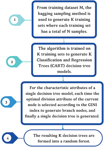
RF was adopted to conduct the LULC classification using Landsat 7, 8, and 9 images. RF is a group of regression trees that grow from the random selection of training data samples (Ali et al. 2012), as outlined in Figure 2. Ma et al. (2017) and Masiliūnas et al. (2021) posited that RF, which improves from the CART algorithm, performs well when classifying remotely sensed imagery. RF can also solve classification and regression problems (Nghia et al. 2021). Thus, it has become the most utilized machine learning algorithm in classifying remote sensing images (Luo et al. 2021).

Figure 2. The formation of RF, as outlined in Chen et al. (2021).

2.4.2. Support vector machines

SVM is one of the most robust pattern recognition methods, which operates by determining an optimal separation line (hyperplane) that accurately separates two or more classes (Bennett-Lenane et al. 2022). Determining the optimal hyperplane maximizes the generalization ability of the SVM model (Cervantes et al. 2020). However, if the data is not linearly separable as in this study, the generalization of the model is hindered. Thus, a kernel function is employed (Saygılı 2022). This study selected the radial basis function (RBF) to perform the LULC classification because it is effective in handling non-linearly separable data as was the case in this study (Anyanwu et al. 2023).

2.4.3. Extreme gradient boosting

XGBoost is an extension of gradient boosting machines (GBMs), a widely employed technique in various remote sensing applications (Buthelezi et al. 2020). Its application has been limited to structural engineering, hence, its limited application in remote sensing (Nguyen et al. 2021). XGBoost model employs additive learning to develop a ‘strong’ learner through the integration of several ‘weak’ learners (Fan et al. 2021). The XGBoost algorithm was developed to a achieve low risk of overfitting and high accuracy (Nguyen et al. 2021).

2.5. Parameter optimisation

RF in RStudio requires parameter optimization, which significantly improves the algorithm’s accuracy (Buthelezi et al. 2020). The performance of RF is primarily influenced by two main parameters: the number of features randomly selected for constructing each tree (Mtry) and the total number of trees to be generated (Ntree). However, it should be noted that only Mtry can be adjusted manually. Therefore, to obtain the optimal Mtry, the expand.grid function in RStudio was used. In the case of SVM, the optimized parameters were the cost (C) and gamma (γ), both of which are independent of each other. A lower value of C places emphasis on maximizing the margin, whereas a higher value indicates a preference for minimizing errors in the SVM algorithm. The γ relates to how much curvature is required in a decision boundary. When the γ parameter is low, it means the single training sample is far-reaching, whereas when it is high, the opposite is true. Optimized parameters for RF and SVM are presented in Table 3.

Table 3. Optimized parameters for both RF and SVM.

RF Parameter	Value	SVM Parameter	Value
Mtry	1	Cost (C)	1
Ntree	1	Gamma (γ)	0.083

XGBoost requires multiple parameters to be optimized, among them; the number of trees, learning rate, and regularization parameters (Nguyen et al. 2021). The Bayesian optimization method, outlined in Bergstra et al. (2011), was utilized to obtain optimal parameters for XGBoost, and the resulting parameter values are presented in Table 4.

Table 4. XGBoost optimal parameters that were obtained using the Bayesian optimization method.

XGBoost Parameter	Value
Subsample Ratio (rs)	1
Learning Rate (τ)	0.3
Maximum Tree Depth (Dmax)	6
Minimum Child Weight (ωmc)	1
Column subsample ratio (rc)	0.9471

2.6. Variable importance

Variable importance for RF and XGBoost LULC classifications was determined using the importance and varImp functions in RStudio, respectively. RF’s variable importance can be presented using the permutation-based metric and a node impurity metric. The node impurity metric (mean decrease in Gini coefficient) was used for this study. It is defined as the average of a variable’s total decrease in node impurities after the splitting of the variable, averaged over all trees (Luo et al. 2021). For XGBoost, the relative importance (RI) score, which is also based on the Gini coefficient importance, was used (Kardani et al. 2022). RI for this study was scaled from 0 to 100. Given that SVM used RBF to perform the LULC classification, it was impossible to determine variable importance for the algorithm. That is because, in kernels other than the linear kernel, the separating plane exists in another space because of the kernel transformation of the original space.

2.7. Accuracy assessment

The primary evaluation of LULC classifications involved assessing overall accuracy, user’s accuracy, and producer’s accuracy derived from the confusion matrix, along with calculating of the area under the curve (AUC). The accuracy measures can be calculated in RStudio. The overall accuracy assesses the number of pixels correctly classified within the image and was employed as the primary metric in this study. The producer’s accuracy measures the precision with which reference pixels are classified, while the user’s accuracy assesses how accurately the classified map reflects the actual conditions on the ground (Patel and Kaushal 2010). The AUC is a measure of sensitivity and specificity over all possible threshold values (Halimu et al. 2019).

Furthermore, quantity and allocation disagreements were computed in RStudio and used to investigate the accuracy of the classifications further. Quantity disagreement measures the disparity in the quantity of a specific class of objects between the classified and reference maps, while allocation disagreement compares the spatial arrangement of pixels between the classified and reference maps (Pontius and Millones 2011, Fassnacht et al. 2014, Lottering et al. 2020, Verma et al. 2020). The allocation disagreement in this study uses the exchange and shift measures. Exchange occurs when a pair of pixels is classified as category A in the reference map and as category B in the classified map, and vice versa (Pontius and Santacruz 2014). Whereas shift is a measure of allocation disagreement used when comparing maps with more than two categories, which identifies situations where the spatial distribution of classes differs between the maps. Still, these differences are not due to a simple exchange of categories (e.g. forest classified as water in the reference map and water classified as forest in the classified map) (Bontempo et al. 2020).

2.8. Percentage area for each class

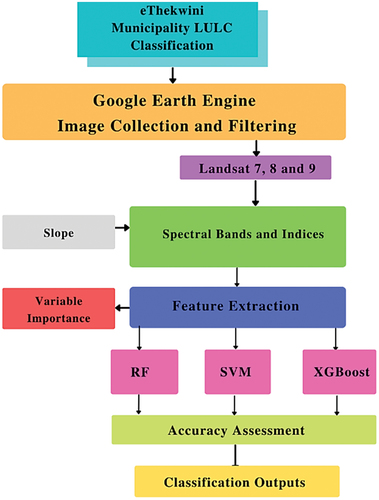
The LULC classification outputs were investigated in QGIS Desktop 3.26.1 for the quantity of the pixels belonging to each class using the raster layer unique values report tool. The values from the report were used to compute the percentages for the area occupied by each LULC class within the study area. The overall methodology is outlined in Figure 3.

Figure 3. The overall framework used to perform RF, SVM, and XGBoost LULC classifications.

3. Results

3.1. Variable importance

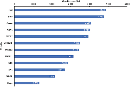
Figure 4 shows the variable importance for RF LULC classifications based on the 2017 Landsat 8 image classification. The figure indicated that the red and blue bands were the most important variables, whereas slope had the least importance. When comparing the importance of spectral indices used in RF classifications, NDVI was the most important index.

Figure 4. Variable importance based on the mean decrease in the Gini coefficient for RF LULC classification on the 2017 Landsat 8 image.

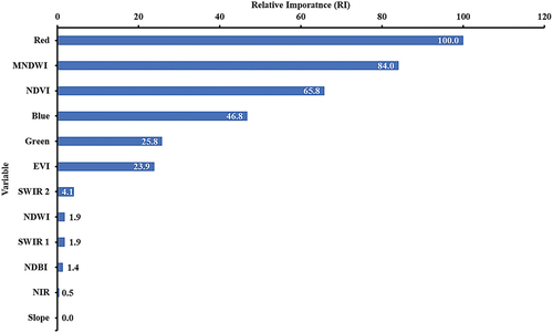
When XGBoost was used to perform LULC classification on the 2017 Landsat image, the red band and MNDWI were the most prioritized variables (Figure 5). Like in RF, the slope was the least prioritized variable.

Figure 5. Variable importance based on the RI for XGBoost LULC classification on the 2017 Landsat 8 image.

3.2. Accuracy assessment

3.2.1. Confusion matrix

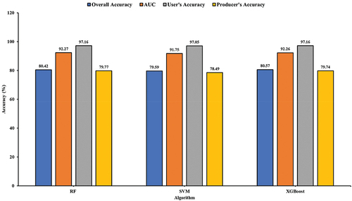
All three algorithms successfully classified the 2017 Landsat 8 image in RStudio. However, these classifications were executed at varying accuracies (Figure 6). Based on the overall accuracy for RF, SVM and XGBoost LULC classifications performed on Landsat images, it was observed that XGBoost classifications (80.57%) performed slightly better than RF (80.42%) and SVM (79.59%). Based on the user’s accuracy RF and XGBoost (97.16%) outperformed SVM (97.05%). However, RF (92.27%) did perform fractionally better than XGBoost (92.26%) and SVM (91.75%) based on the AUC measure. RF (79.77%) also performed better than XGBoost (79.74%) and SVM (78.49%) based on the producer’s accuracy.

Figure 6. RF, SVM and XGBoost classification accuracies based on the overall accuracy, user’s accuracy, producer’s accuracy, and AUC measures from the 2017 Landsat 8 image.

3.2.2. Quantity and allocation disagreements

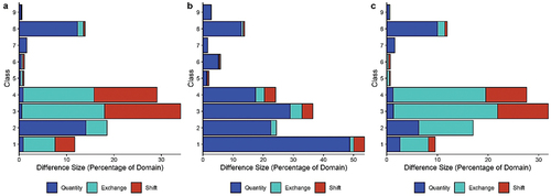
Figure 7 shows the results for disagreement metrics which represent the percentage of disagreement between LULC maps classified based on the 2017 Landsat 8 images and the reference map. The exchange and shift represent the percentage of allocation disagreement. RF LULC classification had a quantity disagreement of 15.72%, an exchange of 22.79% and a shift of 17.28% (Figure 7(a)). The quantity disagreement observed in the RF classification was significantly less than that observed in the SVM classification (Figure 7(b)), which was 70.66%. However, SVM performed better than RF when looking at the exchange and shift measures, which were 5.50% and 6.22%, respectively. Overall, XGBoost performed better than RF and SVM with a quantity disagreement of 11.92%, an exchange of 28.73% and a shift of 10.29% (Figure 7(c))

Figure 7. Disagreement metrics for the (a) RF, (b) SVM and (c) XGBoost LULC classification maps based on the 2017 Landsat 8 image.

Overall, XGBoost produced slightly more accurate classifications than RF and SVM. Hence, it was selected to map LULC change within the eThekwini Municipality.

3.3. Class area distribution

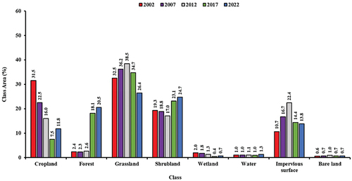
Figure 8 illustrates the changing landscape dynamics within the study area from 2002 to 2022. Over this period, notable trends include a consistent decline in cropland area from 31.5% in 2002 to 7.5% in 2017, followed by a slight increase to 11.8% in 2022, indicating potential shifts in agricultural practices or land use conversions. Forest cover remained relatively stable until 2017, experiencing a significant increase to 20.5% in 2022, possibly reflecting afforestation efforts or natural regeneration processes. Grassland areas fluctuated, peaking at 38.5% in 2012 before declining to 26.4% in 2022, suggesting changes in land management or ecological processes. Shrubland habitats remained consistent until 2017, with a slight expansion to 24.7% in 2022. Wetland and water areas showed minimal changes, indicating stable hydrological conditions. Impervious surface areas peaked in 2012 at 22.4% before declining to 13.8% in 2022, possibly reflecting urbanization patterns. Bare land areas remained relatively stable, suggesting minimal changes in this class.

Figure 8. Comparison of the area covered by each class after classifying all the Landsat images using XGBoost.

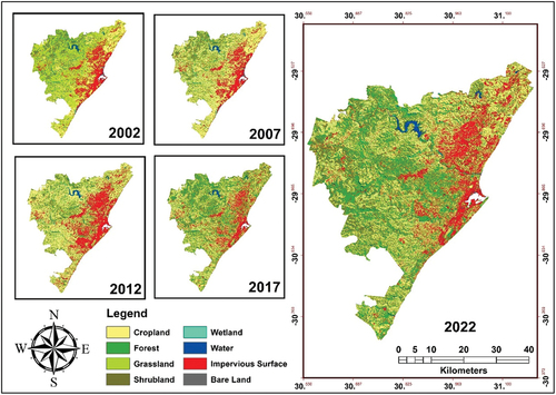
However, it was observed that when XGBoost classified Landsat 7 images, forest vegetation was underestimated compared to its classification of Landsat 8 and 9 images. Conversely, Landsat 8 and 9 classifications exhibited an underestimation of impervious surfaces compared to Landsat 7. Given the improved radiometric resolution in Landsat 9, the final 2022 classification was accepted and presented in Figure 9. Impervious surfaces are found in the eastern and northern parts of the eThekwini Municipality. Vegetated landscapes are found mainly in the western part of the municipality. It was also observed that forested areas are mostly fragmented. Fragmentation of forested areas was observed through the discontinuous distribution of forest patches, with numerous small and isolated patches scattered across the landscape.

Figure 9. The spatial arrangement of LULC classes within the eThekwini Municipality from 2002 to 2022.

4. Discussion

Improved access to medium and high-resolution remote sensing data coupled with free cloud-based geospatial analysis platforms such as GEE has enabled large-scale LULC classifications to be conducted more efficiently (Tassi and Vizzari 2020). Machine learning algorithms have also gained more interest in remote sensing studies because they have outperformed most conventional parametric techniques (Ngolo and Watanabe 2022). Therefore, this study utilized Landsat data from GEE to map LULC change using RF, SVM and XGBoost from 2002 to 2022 for the eThekwini Municipality. The performance of these algorithms was compared using mainly the overall accuracy extracted from the confusion matrix and quantity and allocation disagreements where XGBoost produced the highest overall accuracy.

This is consistent with conclusions in recent research findings such as Pan (2018), who compared the performance of XGBoost in predicting the concentration of 2.5 µm aerosol particles (PM2.5) in the air with artificial neural networks (ANNs), RF, multiple linear regression (MLR) and SVM. XGBoost was found to have outperformed all the other algorithms based on the root-mean-square error (RMSE) (17.298) and R² (0.9520). Yu et al. (2021) investigated the performance of XGBoost, RF and SVM in mapping the vertical forest structure, where it was observed that XGBoost (0.92) performed better than RF (0.90) and SVM (0.90) based on the F1 Score. In their study, Geng et al. (2021) applied RF, SVM, ANN, and XGBoost to predict seasonal maize biomass using field observation data and imagery from the Moderate-Resolution Imaging Spectroradiometer (MODIS). They found that XGBoost (0.77) and RF (0.77) performed better than ANN (0.72) and SVM (0.72) based on the R².

The advantage of XGBoost over other algorithms is based on its ability to reduce inaccuracies resulting from over- and underestimation and corrects the residual error, which results from the generation of a new tree based on the previous tree (Li et al. 2019, Geng et al. 2021). XGBoost can also accurately classify noisy data due to its loss function flexibility (Izadi et al. 2021). However, it should be noted that the performances of both RF and SVM were not significantly lower than that of XGBoost. Furthermore, when the performance of the three algorithms was investigated using the AUC, RF performed better than both XGBoost and SVM. This meant all algorithms used in this study could perform LULC classifications on a regional scale.

This study further evaluated the importance of variables used to classify LULC change. However, it should be noted that variable importance could not be extracted in RStudio for SVM, due to applying the RBF kernel. That is because, in a non-linear kernelised SVM, the separating plane exists in another space because of the kernel transformation of the original space. In RF classifications, the top four variables in terms of importance were the red band, blue band, green band and NDVI. The red and green bands provide critical information for detecting vegetation, given their sensitivity to a wider range of chlorophyll concentrations (Odebiri et al. 2022). Landsat’s green band is positioned above the green edge, a range of wavelengths where vegetation’s reflectance behavior changes, similar to the red band and red edge, both of which shift toward longer wavelengths in areas with high chlorophyll concentration due to chlorophyll’s absorption properties, serving as a crucial indicator of healthy and dense vegetation in remote sensing (Pastor-Guzman et al. 2015). Pastor-Guzman et al. (2015) added that as chlorophyll concentration increases, the red spectral band would reach minimum reflectance, whereas the green band continues to be sensitive. The blue band is useful in differentiating deciduous from coniferous vegetation and overall vegetation from bare soil (Li et al. 2019). NDVI is calculated using the red band and NIR and is a measure of vegetation greenness and health of vegetation in each pixel in a remotely sensed image (Kumar et al. 2022). This meant RF was more efficient at discriminating vegetation from other classes when performing LULC classifications.

The red band was also the most important variable in the XGBoost classification, followed by MNDWI, NDVI and the blue band. The MNDWI improves on the NDWI, which helps detect hydrological changes (Teng et al. 2021). It was successfully employed by Pal and Pani (2016) to detect changes in the Ganga River water surface coverage in India. MNDWI uses green and SWIR bands to detect open water features and to discriminate them from impervious surface features as these are often correlated in other indices (Zhang and Liu 2022). NDVI and the blue are critical for vegetation detection. This meant XGBoost was more efficient at discriminating vegetation and water bodies from other classes.

Given its better performance, the images classified using XGBoost were investigated for the area covered by each class within the study area boundary. The results showed that cropland, grassland, shrubland and impervious surfaces dominated the eThekwini Municipality landscape. Classifications also revealed that cropland, shrubland, and water exhibited a decreasing trend from 2002 to 2017, while grassland and impervious surface classes experienced an increase from 2002 to 2012. In 2022, cropland accounted for 11.8%, forest for 20.5%, grassland for 26.4%, shrubland for 24.7%, wetland for 0.7%, water for 1.3%, and impervious surface for 13.8% of the total land cover within the eThekwini Municipality. However, it should be noted that when XGBoost classified Landsat 7 images, it was observed that it underestimated forest vegetation compared to when it classified Landsat 8 and Landsat 9 images, which also underestimated the impervious surface compared to Landsat 7. This meant it was impossible to determine the extent of the increase in impervious surfaces after 2012. However, the improved radiometric resolution of Landsat 8 and Landsat 9 over Landsat 7 provided enhanced spatial and radiometric details (Mushore et al. 2022). Therefore, it was concluded that outputs from classified Landsat 8 and Landsat 9 images were more representative of the spatial arrangement of the eThekwini Municipality.

The 2022 LULC map output showed that impervious surfaces were most prevalent along the coast, which was along the eastern side of the eThekwini Municipality. Cropland was prevalent in the northern part of the municipality, where Tongaat Hulett, a sugar and maize company is, a major landowner (Moffett and Freund 2004). However, during the 1990s, Tongaat Hulett diversified its operations to include land management and property development, resulting in notable projects like gated townhouses, holiday complexes, shopping centers, and the establishment of the King Shaka International Airport in the region (Todes 2014). Hence, impervious areas have been expanding toward the north.

It was also mentioned in this study that the eThekwini Municipality is susceptible to adverse environmental consequences due to accelerated spatial change resulting from attempts to rectify inequalities and socioeconomic distortions created by apartheid through infrastructure projects (Sutherland et al. 2014, Musvoto et al. 2016). These government infrastructure projects further contributed to the increase in impervious surfaces and the decrease in vegetated landscapes. These areas are surrounded mainly by croplands, forests, and shrubland. Furthermore, with the projected increase in population numbers within the eThekwini Municipality and infrastructural expansion, it is probable that impervious areas will expand further and, therefore, will reduce the area covered by vegetation (Otunga et al. 2014).

The loss of vegetated landscapes means that natural ecosystem services that are vital for climate change mitigation, such as carbon storage, flood attenuation, and food production from these landscapes, are also lost (Tew 2019). The 2022 LULC map revealed that forested areas exhibit a high degree of fragmentation. Fragmentation in forested areas was observed by identifying discontinuities or breaks in the forest cover across the landscape. This was evident through the presence of isolated patches of forest separated by non-forested areas. Forest fragmentation is often associated with species loss, bird nest parasitism, and increased edge effects, which also result in increased predator density (Slattery and Fenner 2021). Increased predator density significantly impacts biodiversity through increased direct killing of prey and fear of predators, which changes some prey species’ behavioral patterns, physiology and reproduction rate (Yousef et al. 2021).

This study also underscores the significance of Landsat 9 in LULC classification, highlighting its utility and contribution to enhancing the accuracy of classification outcomes (You et al. 2022, Jombo and Adelabu 2023). By incorporating Landsat 9 imagery alongside Landsat 7 and Landsat 8, the study leveraged the improved radiometric resolution of Landsat 9 to refine the classification process, thereby providing more precise and detailed insights into LULC dynamics within the eThekwini Municipality. This aligns closely with findings by Shahfahad et al. (2023) and Ghasempour et al. (2023), who similarly compared the effectiveness of Landsat 8 and Landsat 9 for LULC mapping across a heterogeneous landscape. The successful integration of Landsat 9 underscores its potential as an asset in remote sensing applications, offering enhanced capabilities for monitoring and assessing environmental changes over time.

Therefore, by updating LULC maps for the eThekwini Municipality, this study aids decision-makers in mitigating the persisting challenges of climate change through appropriate environmental management policies and strategies. By applying applicable environmental policies, there will be fewer vegetated landscapes lost. This study also highlighted the applicability of remote sensing, machine learning and GEE data in LULC classifications. The utilization of GEE, in this study, is very significant given the finding by Chaves et al. (2020) that big data processing is still challenging for analysts. GEE eliminates this challenge by allowing analysts to access, analyze and visualize geospatial big data in powerful ways without needing for specialized coding expertise or supercomputers (Tamiminia et al. 2020). This study also employed Landsat 9, which was launched toward the end of 2021. Therefore, this study becomes one of the few studies that have used it for regional LULC classifications.

5. Conclusion

This study successfully classified LULC change for the eThekwini Municipality using machine learning algorithms and Landsat data. The findings illustrated that XGBoost classifications using Landsat imagery could perform better classification than RF and SVM. Therefore, the eThekwini Municipality’s LULC change was mapped using XGBoost and Landsat imagery. The produced maps will aid decision-makers in making socioeconomically sound plans that do not infringe on the environment. It is also recommended that the eThekwini Municipality update its LULC maps annually. Future studies can adopt the methodology used in this study to perform accurate LULC classifications. Also, studies that are not financially constrained can utilize high-resolution imagery to perform LULC classifications to improve accuracy.

Disclosure statement

No potential conflict of interest was reported by the author(s).

Data availability statement

The data supporting this study’s findings are available on request from the corresponding author.

Additional information

Funding

This work was supported by the [National Research Foundation of South Africa (NRF) Research Chair in Land Use Planning and Management] under Grant [84157, 127354 and 114898].

References

- Abdi, A.M., 2020. Land cover and land use classification performance of machine learning algorithms in a boreal landscape using Sentinel-2 data. GIScience & Remote Sensing, 57 (1), 1–20. doi:10.1080/15481603.2019.1650447
- Ai, J., et al. 2020. Mapping annual land use and land cover changes in the Yangtze Estuary region using an object-based classification framework and Landsat time series data. Sustainability, 12 (2), 659. doi:10.3390/su12020659
- Ali, J., et al. 2012. Random forests and decision trees. International Journal of Computer Science Issues, 9 (5), 272.
- Ali, U., et al. 2022. Limiting the collection of ground truth data for land use and land cover maps with machine learning algorithms. ISPRS International Journal of Geo-Information, 11 (6), 333. doi:10.3390/ijgi11060333
- Amini, S., Saber, M., Rabiei-Dastjerdi, H., & Homayouni, S., 2022. Urban land use and land cover change analysis using random forest classification of Landsat time series. Remote Sensing, 14 (11), 2654. doi:10.3390/rs14112654
- Anyanwu, G.O., et al. 2023. RBF-SVM kernel-based model for detecting DDoS attacks in SDN integrated vehicular network. Ad Hoc Networks, 140, 103026. doi:10.1016/j.adhoc.2022.103026
- Bennett-Lenane, H., Griffin, B.T., and O’Shea, J.P., 2022. Machine learning methods for prediction of food effects on bioavailability: a comparison of support vector machines and artificial neural networks. European Journal of Pharmaceutical Sciences, 168, 106018. doi:10.1016/j.ejps.2021.106018
- Bergstra, J., et al. 2011. Algorithms for hyper-parameter optimization. In: Proceedings of the 24th international conference on neural information processing systems, 12-15 December Granada, Spain, 2546–2554.
- Bontempo, E., et al. 2020. Classification system drives disagreement among Brazilian vegetation maps at a sample area of the semiarid Caatinga. In: 2020 IEEE Latin American GRSS & ISPRS Remote Sensing Conference (LAGIRS), 22–26 March Santiago, Chile.
- Boon, R., et al. 2016. Managing a threatened savanna ecosystem (KwaZulu- Natal Sandstone Sourveld) in an urban biodiversity hotspot: Durban, South Africa. Bothalia - African Biodiversity & Conservation, 46 (2), 1–12. doi:10.4102/abc.v46i2.2112
- Buchhorn, M., et al. 2020. Copernicus global land cover layers—collection 2. Remote Sensing, 12 (6), 1044. doi:10.3390/rs12061044
- Buthelezi, M.N.M., et al. 2020. Comparing rotation forests and extreme gradient boosting for monitoring drought damage on KwaZulu-Natal commercial forests. Geocarto International, 37 (11), 1–24. doi:10.1080/10106049.2020.1852612
- Buthelezi, M.N.M., et al. 2024. Assessing the extent of land degradation in the eThekwini Municipality using land cover change and soil organic carbon. International Journal of Remote Sensing, 45 (4), 1339–1367. doi:10.1080/01431161.2024.2307945
- Cao, H., Han, L., and Li, L., 2022. Harmonizing surface reflectance between Landsat-7 ETM + , Landsat-8 OLI, and Sentinel-2 MSI over China. Environmental Science and Pollution Research, 29 (47), 70882–70898. doi:10.1007/s11356-022-20771-4
- Cervantes, J., et al. 2020. A comprehensive survey on support vector machine classification: applications, challenges and trends. Neurocomputing, 408, 189–215. doi:10.1016/j.neucom.2019.10.118
- Chakraborty, A., Sachdeva, K., and Joshi, P.K., 2016. Mapping long-term land use and land cover change in the central Himalayan region using a tree-based ensemble classification approach. Applied Geography, 74, 136–150. doi:10.1016/j.apgeog.2016.07.008
- Chander, G., Markham, B.L., and Helder, D.L., 2009. Summary of current radiometric calibration coefficients for Landsat MSS, TM, ETM+, and EO-1 ALI sensors. Remote Sensing of Environment, 113 (5), 893–903. doi:10.1016/j.rse.2009.01.007
- Chaves, M.E.D., Picoli, M.C.A., and Sanches, L.D., 2020. Recent applications of Landsat 8/OLI and Sentinel-2/MSI for land use and land cover mapping: a systematic review. Remote Sensing, 12 (18), 3062. doi:10.3390/rs12183062
- Chen, J., et al. 2015. Global land cover mapping at 30m resolution: a POK-based operational approach. ISPRS Journal of Photogrammetry & Remote Sensing, 103, 7–27. doi:10.1016/j.isprsjprs.2014.09.002
- Chen, Y., et al. 2021. Large group activity security risk assessment and risk early warning based on random forest algorithm. Pattern Recognition Letters, 144, 1–5. doi:10.1016/j.patrec.2021.01.008
- Digra, M., Dhir, R., and Sharma, N., 2022. Land use land cover classification of remote sensing images based on the deep learning approaches: a statistical analysis and review. Arabian Journal of Geosciences, 15 (10), 1003. doi:10.1007/s12517-022-10246-8
- Effiong, C., Ngang, E., and Ekott, I., 2024. Land use planning and climate change adaptation in river-dependent communities in Nigeria. Environmental Development, 49, 100970. doi:10.1016/j.envdev.2024.100970
- Fan, J., et al. 2021. Estimation of daily maize transpiration using support vector machines, extreme gradient boosting, artificial and deep neural networks models. Agricultural Water Management, 245, 106547. doi:10.1016/j.agwat.2020.106547
- Fassnacht, F.E., et al. 2014. Comparison of feature reduction algorithms for classifying tree species with hyperspectral data on three central European test sites. IEEE Journal of Selected Topics in Applied Earth Observations & Remote Sensing, 7 (6), 2547–2561. Article 6851112. doi:10.1109/JSTARS.2014.2329390
- Gao, B.-C., 1996. NDWI—a normalized difference water index for remote sensing of vegetation liquid water from space. Remote Sensing of Environment, 58 (3), 257–266. doi:10.1016/S0034-4257(96)00067-3
- Geng, L., et al. 2021. Corn biomass estimation by integrating remote sensing and long-term observation data based on machine learning techniques. Remote Sensing, 13 (12), 2352. doi:10.3390/rs13122352
- Ghasempour, F., Sekertekin, A., and Kutoglu, S.H., 2023. How Landsat 9 is superior to Landsat 8: Comparative assessment of land use land cover classification and land surface temperature. ISPRS Annals of the Photogrammetry, Remote Sensing & Spatial Information Sciences, X-4/W1-2022, 221–227. doi:10.5194/isprs-annals-X-4-W1-2022-221-2023
- González-González, A., Clerici, N., and Quesada, B., 2022. A 30 m-resolution land use-land cover product for the Colombian andes and amazon using cloud-computing. International Journal of Applied Earth Observation and Geoinformation, 107, 102688. doi:10.1016/j.jag.2022.102688
- Gorelick, N., et al. 2017. Google Earth engine: planetary-scale geospatial analysis for everyone. Remote Sensing of Environment, 202, 18–27. doi:10.1016/j.rse.2017.06.031
- Gross, G., et al. 2022. Initial cross-calibration of Landsat 8 and Landsat 9 using the simultaneous underfly event. Remote Sensing, 14 (10). doi:10.3390/rs14102418
- Halimu, C., Kasem, A., and Newaz, S.H.S., 2019. Empirical comparison of area under ROC curve (AUC) and Mathew correlation coefficient (MCC) for evaluating machine learning algorithms on imbalanced datasets for binary classification. In: Proceedings of the 3rd international conference on machine learning and soft computing. Da Lat, Viet Nam. doi:10.1145/3310986.3311023
- He, C., et al. 2010. Improving the normalized difference built-up index to map urban built-up areas using a semiautomatic segmentation approach. Remote Sensing Letters, 1 (4), 213–221. doi:10.1080/01431161.2010.481681
- Hellberg, S., 2014. Water, life and politics: exploring the contested case of eThekwini Municipality through a governmentality lens. Geoforum; Journal of Physical, Human, and Regional Geosciences, 56, 226–236. doi:10.1016/j.geoforum.2014.02.004
- Huete, A., et al. 2002. Overview of the radiometric and biophysical performance of the MODIS vegetation indices. Remote Sensing of Environment, 83 (1–2), 195–213. doi:10.1016/S0034-4257(02)00096-2
- Izadi, M., et al. 2021. A remote sensing and machine learning-based approach to forecast the onset of harmful algal bloom. Remote Sensing, 13 (19), 3863. doi:10.3390/rs13193863
- Jombo, S. and Adelabu, S., 2023. Evaluating Landsat-8, Landsat-9 and Sentinel-2 imageries in land use and land cover (LULC) classification in a heterogeneous urban area. Geo Journal, 88 (1), 377–399. doi:10.1007/s10708-023-10982-8
- Kafy, A.A., et al. 2021. Remote sensing approach to simulate the land use/land cover and seasonal land surface temperature change using machine learning algorithms in a fastest-growing megacity of Bangladesh. Remote Sensing Applications: Society & Environment, 21, 100463. doi:10.1016/j.rsase.2020.100463
- Kardani, N., et al. 2022. Experimental study and machine learning aided modelling of the mechanical behaviour of rammed earth. Geotechnical and Geological Engineering, 40 (10), 5007–5027. doi:10.1007/s10706-022-02196-5
- Khumalo, N.Z. and Sibanda, M., 2019. Does urban and peri-urban agriculture contribute to household food security? An assessment of the food security status of households in Tongaat, eThekwini Municipality. Sustainability, 11 (4), 1082. doi:10.3390/su11041082
- Kumar, B.P., et al. 2022. Geo-environmental monitoring and assessment of land degradation and desertification in the semi-arid regions using Landsat 8 OLI/TIRS, LST, and NDVI approach. Environmental Challenges, 8, 100578. doi:10.1016/j.envc.2022.100578
- Li, L., et al. 2019. Mapping Moso bamboo forest and its on-year and off-year distribution in a subtropical region using time-series Sentinel-2 and Landsat 8 data. Remote Sensing of Environment, 231, 111265. doi:10.1016/j.rse.2019.111265
- Li, Q., et al. 2020. Mapping the land cover of Africa at 10 m resolution from multi-source remote sensing data with Google Earth engine. Remote Sensing, 12 (4), 602. doi:10.3390/rs12040602
- Liang, S., et al. 2022. Accurate monitoring of submerged aquatic vegetation in a macrophytic lake using time-series Sentinel-2 images. Remote Sensing, 14 (3), 640. doi:10.3390/rs14030640
- Lottering, R.T., et al. 2020. Comparing partial least squares (PLS) discriminant analysis and sparse PLS discriminant analysis in detecting and mapping Solanum mauritianum in commercial forest plantations using image texture. ISPRS Journal of Photogrammetry & Remote Sensing, 159, 271–280. doi:10.1016/j.isprsjprs.2019.11.019
- Luo, C., et al. 2021. Using time series Sentinel-1 images for object-oriented crop classification in Google Earth engine. Remote Sensing, 13 (4), 561. doi:10.3390/rs13040561
- Ma, L., et al. 2017. A review of supervised object-based land-cover image classification. ISPRS Journal of Photogrammetry & Remote Sensing, 130, 277–293. doi:10.1016/j.isprsjprs.2017.06.001
- Masiliūnas, D., et al. 2021. Global land characterisation using land cover fractions at 100 m resolution. Remote Sensing of Environment, 259, 112409. doi:10.1016/j.rse.2021.112409
- Moffett, S. and Freund, B., 2004. Elite formation and elite bonding: social structure and development in Durban. Urban Forum, 15 (2), 134–161. doi:10.1007/s12132-004-0017-1
- Moradpour, H., et al. 2020. Landsat-7 and ASTER remote sensing satellite imagery for identification of iron skarn mineralization in metamorphic regions. Geocarto International, 37 (7), 1–28. doi:10.1080/10106049.2020.1810327
- Musetsho, K.D., Chitakira, M., and Nel, W., 2021. Mapping land-use/Land-cover change in a critical biodiversity area of South Africa. International Journal of Environmental Research and Public Health, 18 (19), 10164. doi:10.3390/ijerph181910164
- Mushore, T.D., et al. 2022. Pansharpened Landsat 8 thermal-infrared data for improved land surface temperature characterization in a heterogeneous urban landscape. Remote Sensing Applications: Society & Environment, 26, 100728. doi:10.1016/j.rsase.2022.100728
- Musvoto, G., Lincoln, G., and Hansmann, R., 2016. The role of spatial development frameworks in transformation of the eThekwini Municipality, KwaZulu-Natal, South Africa: reflecting on 20 years of planning. Urban Forum, 27, 187–210. doi:10.1007/s12132-015-9272-6
- Mutanga, O., Adam, E., and Cho, M.A., 2012. High density biomass estimation for wetland vegetation using WorldView-2 imagery and random forest regression algorithm. International Journal of Applied Earth Observation and Geoinformation, 18, 399–406. doi:10.1016/j.jag.2012.03.012
- Mutanga, O. and Kumar, L., 2019. Google Earth engine applications. Remote Sensing, 11 (5), 591. doi:10.3390/rs11050591
- Nasiri, V., et al. 2022. Land use and land cover mapping using Sentinel-2, Landsat-8 satellite images, and Google Earth engine: a comparison of two composition methods. Remote Sensing, 14 (9), 1977. doi:10.3390/rs14091977
- Nghia, N.V., et al. 2021. Object-based land cover classification of the Vu Gia – Thu Bon river basin on the cloud computing platform. Journal of Physics: Conference Series, 1809 (1), 012039. doi:10.1088/1742-6596/1809/1/012039
- Ngolo, A.M.E. and Watanabe, T., 2022. Integrating geographical information systems, remote sensing, and machine learning techniques to monitor urban expansion: an application to Luanda, Angola. Geo-Spatial Information Science, 26 (3), 1–19. doi:10.1080/10095020.2022.2066574
- Nguyen, H.D., Truong, G.T., and Shin, M., 2021. Development of extreme gradient boosting model for prediction of punching shear resistance of r/c interior slabs. Engineering Structures, 235, 112067. doi:10.1016/j.engstruct.2021.112067
- Nkundabose, J.P., 2021. Employing remote sensing tools for assessment of land use/land cover (LULC) changes in Eastern Province, Rwanda. American Journal of Remote Sensing, 9 (1), 23–32. doi:10.11648/j.ajrs.20210901.13
- Odebiri, O., Mutanga, O., and Odindi, J., 2022. Deep learning-based national scale soil organic carbon mapping with Sentinel-3 data. Geoderma, 411, 115695. doi:10.1016/j.geoderma.2022.115695
- Otunga, C., Odindi, J., and Mutanga, O., 2014. Land use land cover change in the fringe of eThekwini Municipality: implications for urban green spaces using remote sensing. South African Journal of Geomatics, 3 (2), 145–162. doi:10.4314/sajg.v3i2.3
- Pal, R. and Pani, P., 2016. Seasonality, barrage (Farakka) regulated hydrology and flood scenarios of the Ganga River: a study based on MNDWI and simple Gumbel model. Modeling Earth Systems and Environment, 2 (2), 57. doi:10.1007/s40808-016-0114-x
- Pan, B., 2018. Application of XGBoost algorithm in hourly PM2.5 concentration prediction. IOP Conference Series: Earth and Environmental Science, 113, 012127. doi:10.1088/1755-1315/113/1/012127
- Pastor-Guzman, J., et al. 2015. Spatiotemporal variation in mangrove chlorophyll concentration using Landsat 8. Remote Sensing, 7 (11), 14530–14558. doi:10.3390/rs71114530
- Patel, N. and Kaushal, B.K., 2010. Improvement of user’s accuracy through classification of principal component images and stacked temporal images. Geo-Spatial Information Science, 13 (4), 243–248. doi:10.1007/s11806-010-0380-0
- Pontius, R.G. and Millones, M., 2011. Death to Kappa: birth of quantity disagreement and allocation disagreement for accuracy assessment. International Journal of Remote Sensing, 32 (15), 4407–4429. doi:10.1080/01431161.2011.552923
- Pontius, R.G. and Santacruz, A., 2014. Quantity, exchange, and shift components of difference in a square contingency table. International Journal of Remote Sensing, 35 (21), 7543–7554. doi:10.1080/2150704X.2014.969814
- Qiu, J., et al. 2018. A comparison of NDVI and EVI in the DisTrad model for thermal sub-pixel mapping in densely vegetated areas: a case study in Southern China. International Journal of Remote Sensing, 39 (8), 2105–2118. doi:10.1080/01431161.2017.1420929
- Qu, L.A., et al. 2021. Accuracy improvements to pixel-based and object-based LULC classification with auxiliary datasets from Google Earth engine. Remote Sensing, 13 (3), 453. doi:10.3390/rs13030453
- Raut, S.K., Chaudhary, P., and Thapa, L., 2020. Land use/land cover change detection in Pokhara Metropolitan, Nepal using remote sensing. Journal of Geoscience and Environment Protection, 8 (8), 25–35. doi:10.4236/gep.2020.88003
- Roy, D.P., et al. 2016. Characterization of Landsat-7 to Landsat-8 reflective wavelength and normalized difference vegetation index continuity. Remote Sensing of Environment, 185, 57–70. doi:10.1016/j.rse.2015.12.024
- Santra, A., et al. 2021. Identification of impervious built-up surface features using ResourceSat-2 LISS-III-Based novel optical built-up index. In: P. Kumar, H. Sajjad, B.S. Chaudhary, J.S. Rawat, and M. Rani, eds. Remote sensing and GIScience: challenges and future directions. Springer International Publishing, 113–126. doi:10.1007/978-3-030-55092-9_7
- Saygılı, A., 2022. Computer-aided detection of COVID-19 from CT images based on Gaussian mixture model and kernel support vector machines classifier. Arabian Journal for Science & Engineering, 47 (2), 2435–2453. doi:10.1007/s13369-021-06240-z
- Shahfahad, et al. 2022. Modelling urban heat island (UHI) and thermal field variation and their relationship with land use indices over Delhi and Mumbai metro cities. Environment, Development, and Sustainability, 24 (3), 3762–3790. doi:10.1007/s10668-021-01587-7
- Shahfahad, et al. 2023. Comparative evaluation of operational land imager sensor on board Landsat 8 and Landsat 9 for land use land cover mapping over a heterogeneous landscape. Geocarto International, 38 (1), 2152496. doi:10.1080/10106049.2022.2152496
- Shivambu, T.C., Shivambu, N., and Downs, C.T., 2020. Population estimates of non-native rose-ringed parakeets Psittacula krameri (Scopoli, 1769) in the Durban Metropole, KwaZulu-Natal Province, South Africa. Urban Ecosystems, 24 (4), 649–659. doi:10.1007/s11252-020-01066-3
- Showstack, R., 2022. Landsat 9 satellite continues half-century of earth observations: eyes in the sky serve as a valuable tool for stewardship. BioScience, 72 (3), 226–232. doi:10.1093/biosci/biab145
- Slattery, Z. and Fenner, R., 2021. Spatial analysis of the drivers, characteristics, and effects of forest fragmentation. Sustainability, 13 (6), 3246. doi:10.3390/su13063246
- Sutherland, C., et al. 2014. Water and sanitation provision in eThekwini Municipality: a spatially differentiated approach. Environment and Urbanization, 26 (2), 469–488. doi:10.1177/0956247814544871
- Tadese, M., et al. 2020. Mapping of land-use/land-cover changes and its dynamics in Awash River Basin using remote sensing and GIS. Remote Sensing Applications: Society & Environment, 19, 100352. doi:10.1016/j.rsase.2020.100352
- Talukdar, S., et al. 2020. Land-use land-cover classification by machine learning classifiers for satellite observations—a review. Remote Sensing, 12 (7), 1135. doi:10.3390/rs12071135
- Tamiminia, H., et al. 2020. Google Earth engine for geo-big data applications: a meta-analysis and systematic review. Isprs Journal of Photogrammetry & Remote Sensing, 164, 152–170. doi:10.1016/j.isprsjprs.2020.04.001
- Tassi, A. and Vizzari, M., 2020. Object-oriented LULC classification in Google Earth engine combining SNIC, GLCM, and machine learning algorithms. Remote Sensing, 12 (22), 3776. doi:10.3390/rs12223776
- Teng, J., et al. 2021. Assessing habitat suitability for wintering geese by using normalized difference water index (NDWI) in a large floodplain wetland, China. Ecological Indicators, 122, 107260. doi:10.1016/j.ecolind.2020.107260
- Tew, E.R., 2019. Forests of the future: ecosystem services in a forest landscape facing significant changes. Cambridge, England: University of Cambridge.
- Todes, A., 2014. New African suburbanisation? Exploring the growth of the northern corridor of eThekwini/KwaDakuza. African Studies, 73 (2), 245–270. doi:10.1080/00020184.2014.925188
- Trujillo-Jiménez, M.A., et al. 2022. SatRed: new classification land use/land cover model based on multi-spectral satellite images and neural networks applied to a semiarid valley of Patagonia. Remote Sensing Applications: Society & Environment, 26, 100703. doi:10.1016/j.rsase.2022.100703
- Tucker, C.J. and Sellers, P.J., 1986. Satellite remote sensing of primary production. International Journal of Remote Sensing, 7 (11), 1395–1416. doi:10.1080/01431168608948944
- Vanhellemont, Q., 2020. Combined land surface emissivity and temperature estimation from Landsat 8 OLI and TIRS. ISPRS Journal of Photogrammetry & Remote Sensing, 166, 390–402. doi:10.1016/j.isprsjprs.2020.06.007
- Verma, P., et al. 2020. Appraisal of kappa-based metrics and disagreement indices of accuracy assessment for parametric and nonparametric techniques used in LULC classification and change detection. Modeling Earth Systems and Environment, 6 (2), 1–15. doi:10.1007/s40808-020-00740-x
- Wang, Q., et al. 2021. Filling gaps in Landsat ETM+ SLC-off images with sentinel-2 MSI images. International Journal of Applied Earth Observation and Geoinformation, 101, 102365. doi:10.1016/j.jag.2021.102365
- Wei, T., et al. 2020. Dynamics of land use and land cover changes in an arid piedmont plain in the middle reaches of the Kaxgar River Basin, Xinjiang, China. ISPRS International Journal of Geo-Information, 9 (2), 87. doi:10.3390/ijgi9020087
- Xu, H., 2006. Modification of normalised difference water index (NDWI) to enhance open water features in remotely sensed imagery. International Journal of Remote Sensing, 27 (14), 3025–3033. doi:10.1080/01431160600589179
- Yin, G., et al. 2017. A comparison of gap-filling approaches for Landsat-7 satellite data. International Journal of Remote Sensing, 38 (23), 6653–6679. doi:10.1080/01431161.2017.1363432
- You, H., et al. 2022. A study on the difference of LULC classification results based on Landsat 8 and Landsat 9 data. Sustainability, 14 (21), 13730. doi:10.3390/su142113730
- Yousef, F.B., Yousef, A., and Maji, C., 2021. Effects of fear in a fractional-order predator-prey system with predator density-dependent prey mortality. Chaos, Solitons & Fractals, 145, 110711. doi:10.1016/j.chaos.2021.110711
- Yu, J.-W., et al. 2021. Forest vertical structure mapping using two-seasonal optic images and LiDAR DSM acquired from UAV platform through random forest, XGBoost, and support vector machine approaches. Remote Sensing, 13 (21), 4282. doi:10.3390/rs13214282
- Zha, Y., Gao, J., and Ni, S., 2003. Use of normalized difference built-up index in automatically mapping urban areas from TM imagery. International Journal of Remote Sensing, 24 (3), 583–594. doi:10.1080/01431160304987
- Zhang, X. and Liu, X., 2022. Comparative study on extraction of banded water and surface water in urban area based on MNDWI. In: 2022 3rd International conference on geology, mapping and remote sensing (ICGMRS), 22–24 April 2022 Zhoushan, China.
- Zhu, L., Jin, G., and Gao, D., 2021. Integrating land-cover products based on ontologies and local accuracy. Information, 12 (6), 236. doi:10.3390/info12060236
- Zhu, X., Liu, D., and Chen, J., 2012. A new geostatistical approach for filling gaps in Landsat ETM+ SLC-off images. Remote Sensing of Environment, 124, 49–60. doi:10.1016/j.rse.2012.04.019
- Zungu, M.M., et al. 2019. Fragment and life-history correlates of extinction vulnerability of forest mammals in an urban-forest mosaic in EThekwini Municipality, Durban, South Africa. Animal Conservation, 22 (4), 362–375. doi:10.1111/acv.12470
- Zungu, M.M., et al. 2020. Effects of landscape context on mammal richness in the urban forest mosaic of EThekwini Municipality, Durban, South Africa. Global Ecology and Conservation, 21, e00878. doi:10.1016/j.gecco.2019.e00878