A business-cycle model with money and banking: the case of Bulgaria (1999–2018)

ABSTRACT

We augment an otherwise standard business cycle model with a richer government sector and add modified cash in advance (CIA) and deposit considerations. In particular, both the cash in advance- and deposit constraints of in earlier work are extended to include private investment and government consumption. Also, part of the purchases are made using credit. This specification is then calibrated to Bulgarian data after the introduction of the currency board (1999–2020), gives a role to money and costly credit in accentuating economic fluctuations. In particular, the modified CIA constraint combines monetary with banking theory, and thus produces a novel mechanism that allows the framework to reproduce better observed variability and correlations among model variables, and those characterising the labour market in particular.

KEYWORDS:

• Business cycles
• modified cash-in-advance (CIA) constraint
• deposit constraint
• costly credit
• Bulgaria

1 Introduction and motivation

It is a well-known fact, e.g. Prescott (1986), that the perfectly competitive (Walrasian) approach to modelling labour markets in real business cycles (RBC) – that is, without money in the setup – does not fit data very well, and thus creates a ‘puzzle’ for neoclassical economists. More specifically, in the standard RBC model the fluctuations in employment are due to movements in labour supply. In other words, households increase hours in the face of a raise in the return on labour, the wage, driven by shocks to technology. Instead, if an RBC model is to fit data better along the labour market dimension shocks that work on labour demand and shift it around would be much better candidates to explain the observed fluctuations in the wage rate, aggregate hours and employment, even for a small economy like Bulgaria.

Therefore, in this paper, we base our modelling approach for the artificial economy with money on a particular empirical regularity in Bulgaria, namely that households predominantly use cash for purchases, while credit is produced by foreign-owned banks, which is the norm in the period following the introduction of the currency board arrangement (1999–2018). We adopt the approach followed by Benk et al. (2010) and Cole (2020) to incorporate a modified cash-in-advance (CIA) constraint and explicit credit production into a monetary-RBC model in order to investigate the quantitative effect of money and credit on business cycle fluctuations in aggregate variables in Bulgaria, and whether it is able to address the ‘labor market puzzle,’ and validate certain labour market facts, while at the same time retain technology as the only shock process.

The rest of the paper is organised as follows: Section 2 describes the model framework and describes the decentralised competitive equilibrium system, Section 3 discusses the calibration procedure, and Section 4 presents the steady-state model solution. Sections 5 proceeds with the out-of-steady-state dynamics of model variables and compares the simulated second moments of theoretical variables against their empirical counterparts. Section 6 concludes the paper.

2 Model setup

There is a representative household, which derives utility out of consumption and leisure. The time available to households can be spent in productive use or as leisure. Households use cash for the majority of their purchases. The government taxes consumption spending and levies a common tax on all income, in order to finance wasteful purchases of government consumption goods, and government transfers. The monetary authority follows an endogenous money supply rule and redistributes all seigniorage back to the household. On the production side, there is a representative firm, which hires labour and utilises capital to produce a homogeneous final good, which could be used for consumption, investment, or government purchases.

2.1 Household problem

Each household maximises expected discounted utility, which is of the form used in Benk et al. (2010):

(1) $U=E_0\sum _{t=0}^{\mathrm{\infty }}{\beta }^t\{ln{c}_t+\eta (1-h_{gt}-h_{qt})\},$(1)

where $E_0$ is the expectation operation conditional on information available as of $t=0$, $0<\beta <1$ is the discount factor, $c_t$ is individual household consumption in period $t$, and $h_{gt}$ are hours worked in the goods sector, while $h_{qt}$ are hours worked in the banking sector. Parameter $\eta >0$ is the weight attached to disutility of work.

The household starts with a positive endowment of physical capital, $k_0$, in period 0, which is rented to the firm at the nominal rental rate $R_t$, that is, before-tax capital income equals $R_t{k}_t$. Therefore, each household can decide to invest in capital to augment the capital stock, which evolves according to the following law of motion:

(2) $k_{t+1}=i_t+(1-\delta )k_t,$(2)

where $0<\delta <1$ is the depreciation rate of physical capital.

In addition to the rental income, the household owns the firm, and thus has a legal claim to the firm’s nominal profit, ${\mathrm{\Pi }}_t$. Lastly, the household works a certain number of hours, which are remunerated at the spot nominal wage rate $W_t$, producing a total nominal labour income of $W_t(h_{gt}+h_{qt})$ in period $t$.

The budget constraint of the aggregate household, expressed in real terms, is then

(3) $(1+{\tau }^c)c_t+k_{t+1}-(1-\delta )k_t+\frac{M_{t+1}}{P_t}\frac{P_{t+1}}{P_{t+1}}+\frac{P_{qt}}{P_t}{q}_t=(1-{\tau }^y)[w_t(h_{gt}+h_{qt})+r_t{k}_t+r_{qt}{d}_t+\frac{{\mathrm{\Pi }}_t}{P_t}]+\frac{M_t}{P_t}+g_t^t$(3)

where ${\tau }^c$ is the tax rate on final consumption, ${\tau }^y$ is the proportional rate on labour and capital income, and $P_t$ is the aggregate price level. $M_t$ denote the nominal quantities of money holdings in period $t$. Money stock is treated like a consumption good, it stores wealth over time. That is why real money balances in period $t$ are $m_t=M_t/P_t$ in period $t+1$ only buy $M_t/P_{t+1}$ (next period purchasing power). Similarly, $w_t=W_t/P_t$, and $r_t=R_t/P_t$ are the real wage and the real interest rate.

The household is assumed to hold equity in the representative bank by making deposits in the bank. Each unit of currency deposited is assumed to buy one share at a price of unity; in return, the household receives the bank’s profit as dividend income proportionally to the number of shares (deposits). The real quantity of deposits is denoted by $d_t$; the dividend per unit of deposits as $r_{qt}$, so the household receives nominal dividend income $P_t{r}_{qt}{q}_t$. The household also pays a banking fee for the provision of costly credit. $P_{qt}$ will denote the nominal price of each unit of credit, and $q_t$ is the real quantity of credit used by the household in exchange; the household pays $P_{qt}{q}_t$ in credit fees, and purchases $P_t{q}_t$ in goods and credit.

Output can be purchased using real money balances or credit, hence the households face the following modified cash-in-advance constraint

(4) $(1+{\tau }^c)c_t+k_{t+1}-(1-\delta )k_t+g_t^c=m_t+q_t,$(4)

so the model will feature an endogenous split: some of the purchases are made on credit, and the rest is financed with cash.

Finally, all cash comes out of bank deposits, and purchases made on credit are repaid at the end of the period out of the same deposits. Total deposits are then equal to the value of output (inclusive of VAT).

(5) $d_t=(1+{\tau }^c)c_t+i_t+g_t^c.$(5)

We set up the Lagrangian of the household’s problem:

(6) $\begin{array}{rl}& L=E_0\sum _{t=0}^{\mathrm{\infty }}{\beta }^t\{ln{c}_t+\eta (1-h_{gt}-h_{qt})-{\lambda }_t[(1+{\tau }^c)c_t+k_{t+1}-(1-\delta )k_t+m_{t+1}(1+{\pi }_{t+1})+\frac{P_{qt}}{P_t}{q}_t\\ & -(1-{\tau }^y)[w_t(h_{gt}+h_{qt})+r_t{k}_t+r_{qt}{d}_t+\frac{{\mathrm{\Pi }}_t}{P_t}]-m_t-g_t^t,]\\ & -{\mu }_t[(1+{\tau }^c)c_t+k_{t+1}-(1-\delta )k_t+g_t^c-m_t-q_t]\\ & -{\varphi }_t[(1+{\tau }^c)c_t+k_{t+1}-(1-\delta )k_t+g_t^c-d_t]\}\end{array}$(6)

where ${\lambda }_t,{\mu }_t,{\varphi }_t$ are the Lagrange multipliers attached to the budget constraint, the CIA constraint, and the deposit constraint. The first-order optimality conditions (FOCs) are as follows:

(7) $c_t:\frac{1}{c_t}=(1+{\tau }^c)({\lambda }_t+{\mu }_t+{\varphi }_t)$(7)

(8) $h_{gt}:\frac{\eta }{1-h_{gt}-h_{qt}}={\lambda }_t(1-{\tau }^y)w_t,$(8)

(9) $h_{qt}:\frac{\eta }{1-h_{gt}-h_{qt}}={\lambda }_t(1-{\tau }^y)w_t,$(9)

(10) $k_{t+1}:{\lambda }_t+{\mu }_t+{\varphi }_t=\beta E_t[{\lambda }_{t+1}[1-\delta +(1-{\tau }^y)r_{t+1}]+{\mu }_{t+1}(1-\delta )+{\varphi }_{t+1}(1-\delta )],$(10)

(11) $m_{t+1}:{\lambda }_t=\beta E_t[\frac{1}{1+{\pi }_{t+1}}({\lambda }_{t+1}+{\mu }_{t+1})],$(11)

(12) $d_t:{\lambda }_t(1-{\tau }^y)r_{qt}+{\varphi }_t=0$(12)

(13) $q_t:{\lambda }_t\frac{P_{qt}}{P_t}={\mu }_t.$(13)

where ${\pi }_{t+1}$ is the inflation rate between periods $t$ and $t+1$. Lastly, the boundary (transversality) conditions for capital, and real money balances are as follows:

(14) $TV{C}_k:\underset{t\to \mathrm{\infty }}{lim}{\beta }^t{\lambda }_t{k}_{t+1}=0$(14)

(15) $TV{C}_m:\underset{t\to \mathrm{\infty }}{lim}{\beta }^t{\lambda }_t{m}_{t+1}=0$(15)

The interpretation of the optimality conditions is standard. In the first, the household equates the marginal utility of consumption, to the VAT adjusted shadow price of wealth and the CIA constraint. The second and third FOCs determine the optimal number of hours worked in the goods and banking sector, respectively, by balancing at the margin the cost and benefit from working.¹ The remaining equations from the original FOCs are standard: for example, the Euler equation for capital stock describes how capital is allocated across any adjacent periods in order to maximise household’s utility. Similarly, the other describes the rule for optimal real money balances, deposits, and credit. The transversality conditions (TVCs) for real cash holdings and physical capital are imposed to rule out explosive solutions.

2.2 Stand-in firm’s problem

There is a stand-in firm in the economy, which uses homogeneous capital and labour to produce a final good, which can be used for consumption, investment, or government purchases, through the following production function:

(16) $y_t=A_t{k}_t^{\alpha }{h}_{gt}^{1-\alpha },$(16)

where $A_t$ denotes the level of total factor productivity in period $t$, $h_t$ are total hours used, and $\alpha$ and $1-\alpha$ are the share of capital and labour, respectively. The firm’s problem, expressed in real terms, is to

(17) $\underset{(k_t,h_{gt})\ge 0}{max}{A}_t{k}_t^{\alpha }{h}_{gt}^{1-\alpha }-r_t{k}_t-w_t{h}_{gt}$(17)

The first-order optimality conditions determining optimal capital, and labour use are

(18) $k_t:\alpha \frac{y_t}{k_t}=r_t,$(18)

(19) $h_{gt}:(1-\alpha )\frac{y_t}{h_{gt}}=w_t.$(19)

Given the results above, it follows that profit is zero in all periods.

2.3 Bank’s problem

There is a representative bank in the model, which extends credit to the household and the government, and credit can be used to purchase commodities. The bank maximises the profit stream subject to the labour costs and the deposit costs of producing the credit.

The production of credit follows the ‘financial intermediation’ approach, as features a constant-returns-to-scale technology. More specifically,

(20) $q_t=A_{qt}{h}_{gt}^{\gamma }{d}_t^{1-\gamma },$(20)

where $A_{qt}$ is the efficiency parameter of the costly credit production, and $0<\gamma <1$ is the share of workers employed in the banking industry.

The bank’s problem is

(21) $\underset{(h_{gt},d_t)}{max}{\mathrm{\Pi }}_{qt}=P_{qt}{q}_t-P_t{w}_t{h}_{qt}-P_t{r}_{qt}{d}_t$(21)

The optimality conditions are:

(22) $h_{gt}:\gamma \frac{P_q}{P_t}\frac{q_t}{h_{qt}}=w_t,$(22)

(23) $d_t:(1-\gamma )\frac{P_q}{P_t}\frac{q_t}{d_t}=r_{qt}.$(23)

Given the results above, it follows that bank’s profit is zero in all periods.

2.4 Monetary authority

In this paper, the monetary authority (central bank) supplies the money aggregate, $M_t$, endogenously. In other words, the money supply will respond to the demand for currency for transaction purposes. All money created (seigniorage) in period $t$ is then distributed to the government, and then to the households in a lump-sum fashion

(24) $M_{t+1}-M_t=T_t,$(24)

where $T_t$ is the lump-sum nominal transfer to the household. In the government budget constraint below, we will assume that the central bank distributes the seigniorage to the Ministry of Finance, which in turn passes it to the household as part of the overall government lump-sum transfer, $g_t^t$.

2.5 Government

In the model setup, the government is levying taxes on labour and capital income, as well as consumption in order to finance spending on government purchases and government transfers. The government budget constraint is as follows:

(25) ${\tau }^c{c}_t+{\tau }^y(w_t{h}_t+r_t{k}_t+r_{qt}{d}_t)=g_t^t+g_t^c$(25)

Tax rates and government consumption-to-output ratio would be chosen to match the average share in data, and government transfers would be determined residually.

2.6 Stochastic process

Total factor productivity, $A_t$, is assumed to follow AR(1) processes in logs, in particular

$ln{A}_{t+1}=(1-{\rho }_a)ln{A}_0+{\rho }_{a}ln{A}_t+{ϵ}_{t+1}^a,$

where $A_0>0$ is steady-state level of the total factor productivity process, $0<{\rho }_a<1$ is the first-order autoregressive persistence parameter and ${ϵ}_t^a\sim iidN(0,{\sigma }_a^2)$ are random shocks to the total factor productivity progress. Hence, the innovations ${ϵ}_t^a$ represent unexpected changes in the total factor productivity process.

2.7 Dynamic competitive equilibrium (DCE)

Given the stochastic process $\{A_t{\}}_{t=0}^{\mathrm{\infty }}$, average tax rates $\{{\tau }^c,{\tau }^y\}$, endowments $(k_0,m_0)$, the decentralised dynamic competitive equilibrium is a list of sequences $\{c_t,i_t,k_t,h_t,m_t,d_t,q_t{\}}_{t=0}^{\mathrm{\infty }}$, a sequence of government purchases and transfers $\{g_t^c,g_t^t{\}}_{t=0}^{\mathrm{\infty }}$, real credit price $\{P_{qt}/P_t{\}}_{t=0}^{\mathrm{\infty }}$, and real input prices $\{w_t,r_t{\}}_{t=0}^{\mathrm{\infty }}$ such that (i) the household maximises its utility function subject to its budget constraint, the CIA constraint, and the deposit constraint; (ii) the representative firm maximises profit; (iii) the representative bank maximises profit; (iv) government budget constraint is balanced in each period; (v) all markets clear.

3 Data and model calibration

To calibrate the model to Bulgarian data, we will focus on the period after the introduction of the currency board (1999–2020). Annual data on output, consumption and investment was collected from National Statistical Institute (2022), while the real interest rate is taken from Bulgarian National Bank (2022). The calibration strategy described in this section follows a long-established tradition in modern macroeconomics: first, the discount factor, $\beta =0.982$, as in Vasilev (2017a), is set to match the steady-state capital-to-output ratio in Bulgaria, $k/y=3.491$. The labour share parameter, $\alpha =0.429$, was obtained from Vasilev (2017b) as the average value of labour income in aggregate output over the period 1999–2014.

The relative weights attached to the utility out of leisure in the household’s utility function, $\eta$, is calibrated to match the fact that in steady-state consumers would supply one-third of their time endowment to working. The share of people working in the banking and finance was estimated to be $\gamma =0.11$, which is as in Benk et al. (2010). Next, the average depreciation rate of physical capital in Bulgaria, $\delta =0.05$, was taken from Vasilev (2015). It was estimated as the average depreciation rate over the period 1999–2014. Similarly, the average income tax rate was set to ${\tau }^y=0.1$, and the tax rate on consumption is set to its value over the period, ${\tau }^c=0.2$. Lastly, as in A. Z. Vasilev (2017c), the process followed by total factor productivity is estimated from the detrended Solow residual series by running an AR(1) regression and saving the residuals. Table 1 summarises the values of all model parameters used in the paper.

Table 1. Model parameters.

Parameter	Value	Description	Method
$\beta$	0.982	Discount factor	Calibrated
$\alpha$	0.429	Capital Share	Data average
$\delta$	0.050	Depreciation rate on physical capital	Data average
$\eta$	0.853	Parameter, disutility of work	Calibrated
$\gamma$	0.110	Share of labour in banking	Data average
${\tau }^c$	0.200	VAT/consumption tax rate	Data average
${\tau }^y$	0.100	Average tax rate on income	Data average
$\kappa$	0.850	Share of purchases made using cash	Calibrated
${\rho }_a$	0.701	AR(1) parameter, total factor productivity	Estimated
${\sigma }_a$	0.044	st.dev, total factor productivity	Estimated

4 Steady-state

Once the values of all model parameters were obtained, the steady-state equilibrium system solved, the ‘big ratios’ can be compared to their averages in Bulgarian data. The results are reported in Table 2 on the next page. (We approximate the economy around zero inflation.) The model matches consumption-to-output ratio by construction; the investment and government purchase ratios are also closely approximated. The shares of income are also identical to those in data, which is an artefact of the assumptions imposed on the functional form of the aggregate production function. Lastly, the after-tax return, net of depreciation, $\tilde{r}=(1-{\tau }^y)r-\delta$, is also very closely captured by the model.

Table 2. Data averages and long-run solution.

Variable	Description	Data	Model
$y$	Steady-state output	N/A	0.568
$c/y$	Consumption-to-output ratio	0.674	0.674
$i/y$	Investment-to-output ratio	0.201	0.175
$g^c/y$	Government cons-to-output ratio	0.159	0.151
$wh/y$	Labour income-to-output ratio	0.571	0.571
$rk/y$	Capital income-to-output ratio	0.429	0.429
$h$	Share of time spent working	0.333	0.333
$\tilde{r}$	After-tax net return on capital	0.056	0.057

5 Out of steady-state model dynamics

Since the model does not have an analytical solution for the equilibrium behaviour of variables outside their steady-state values, we need to solve the model numerically. This is done by log-linearising the original equilibrium (non-linear) system of equations around the steady-state. This transformation produces a first-order system of stochastic difference equations. First, we study the dynamic behaviour of model variables to an isolated shock to the total factor productivity process, and then we fully simulate the model to compare how the second moments of the model perform when compared against their empirical counterparts. Special focus is put on the cyclical behaviour of labour market variables.

5.1 Impulse response analysis

This subsection documents the impulse responses of model variables to a 1% surprise innovation to technology. The impulse response functions (IRFs) are presented in Figure 1.

Figure 1. Impulse responses to a 1% surprise innovation in technology.

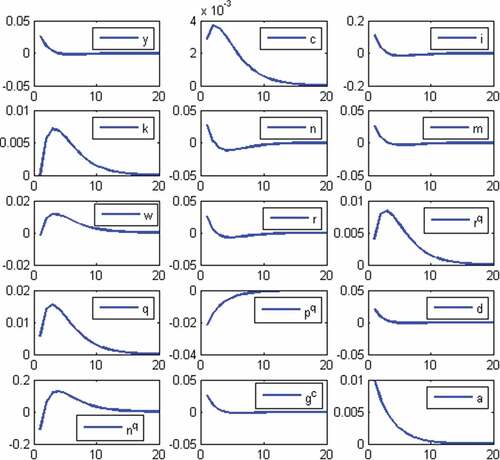
As a result of the one-time unexpected positive shock to total factor productivity, output increases upon impact. This expands the availability of resources in the economy, so uses of output – consumption, investment and government consumption also increase contemporaneously.

At the same time, the jump in productivity increases the after-tax return on the two factors of production, labour and capital. The representative households then respond to the incentives contained in prices and start accumulating capital, and supply more hours worked. In turn, the increase in capital input feeds back in output through the production function and that further adds to the positive effect of the technology shock. In the labour market, the wage rate increases, and the household increases its hours worked. In turn, the increase in total hours further increases output, again indirectly.

Over time, as capital is being accumulated, its after-tax marginal product starts to decrease, which lowers the households’ incentives to save. As a result, physical capital stock eventually returns to its steady-state, and exhibits a hump-shaped dynamics over its transition path. The rest of the model variables return to their old steady-states in a monotone fashion as the effect of the one-time surprise innovation in technology dies out.

5.2 Simulation and moment-matching

We will now simulate the model 10,000 times for the length of the data horizon. Both empirical and model simulated data are detrended using the Hodrick and Prescott (1980) filter. Table 3 on the next page summarises the second moments of data (relative volatilities to output and contemporaneous correlations with output) versus the same moments computed from the model-simulated data at annual frequency.² To minimise the sample error, the simulated moments are averaged out over the computer-generated draws. In addition, we compare the model in this paper (MB Model, short for ‘Money and Banking’ Model) to the benchmark RBC model. Both models match quite well the absolute volatility of output. However, the models substantially overestimate the variability in consumption, and investment. Still, the models are qualitatively consistent with the stylised fact that consumption is less volatile than output, and investment is more volatile than output. By construction, government spending in the model varies as much as in data. With respect to the labour market variables, the variability of employment and wages predicted by the MB model is twice more than that in data.

Table 3. Business cycle moments.

	Data	RBC Model	MB Model
${\sigma }_y$	0.05	0.05	0.05
${\sigma }_c/{\sigma }_y$	0.55	0.63	0.47
${\sigma }_i/{\sigma }_y$	1.77	3.26	3.86
${\sigma }_g/{\sigma }_y$	1.21	1.00	1.00
${\sigma }_h/{\sigma }_y$	0.63	0.63	1.33
${\sigma }_w/{\sigma }_y$	0.83	0.52	1.48
${\sigma }_{y/h}/{\sigma }_y$	0.86	0.52	1.48
$corr(c,y)$	0.85	0.62	0.51
$corr(i,y)$	0.61	0.78	0.85
$corr(g,y)$	0.31	1.00	1.00
$corr(h,y)$	0.49	0.77	0.15
$corr(w,y)$	−0.01	0.66	0.34
$corr(h,y/h)$	−0.14	0.34	−0.62

Next, in terms of contemporaneous correlations, the MB model slightly over-predicts the pro-cyclicality of the main aggregate variables – investment and government consumption while under-predicting the correlations of consumption and hours with output. This, however, is a common limitation of this class of models. With wages, the model predicts a moderate cyclicality (as compared to the strong pro-cyclicality predicted by the RBC model), while wages in data are acyclical.

In the next subsection, we investigate the dynamic correlation between labour market variables at different leads and lags, thus evaluating how well the model matches the phase dynamics among variables. In addition, the autocorrelation functions (ACFs) of empirical data, obtained from an unrestricted VAR(1) are put under scrutiny and compared and contrasted to the simulated counterparts generated from the model.

5.3 Auto- and cross-correlation

This subsection discusses the auto-(ACFs) and cross-correlation functions (CCFs) of the major model variables. The coefficients of empirical ACFs and CCFs at different leads and lags are presented in Table 4 against the simulated AFCs and CCFs. As seen from Table 4 on the next page, the model compares well vis-a-vis data. Empirical ACFs for output and investment are slightly outside the confidence band predicted by the model, while the ACFs for total factor productivity and household consumption are well approximated by the model.

Table 4. Autocorrelations for Bulgarian data and the model economy.

		k
Method	Statistic	0	1	2	3
Data	$corr(h_{gt},h_{g,t-k})$	1.000	0.484	0.009	0.352
Model	$corr(h_{gt},h_{g,t-k})$	1.000	0.815	0.630	0.432
	(s.e.)	(0.000)	(0.039)	(0.071)	(0.097)
Data	$corr(y_t,y_{t-k})$	1.000	0.810	0.663	0.479
Model	$corr(y_t,y_{t-k})$	1.000	0.817	0.627	0.438
	(s.e.)	(0.000)	(0.040)	(0.073)	(0.098)
Data	$corr(a_t,a_{t-k})$	1.000	0.702	0.449	0.277
Model	$corr(a_t,a_{t-k})$	1.000	0.817	0.630	0.443
	(s.e.)	(0.000)	(0.036)	(0.064)	(0.086)
Data	$corr(c_t,c_{t-k})$	1.000	0.971	0.952	0.913
Model	$corr(c_t,c_{t-k})$	1.000	0.817	0.630	0.443
	(s.e.)	(0.000)	(0.035)	(0.064)	(0.087)
Data	$corr(i_t,i_{t-k})$	1.000	0.810	0.722	0.594
Model	$corr(i_t,i_{t-k})$	1.000	0.817	0.626	0.436
	(s.e.)	(0.000)	(0.037)	(0.068)	(0.094)
Data	$corr(w_t,w_{t-k})$	1.000	0.760	0.783	0.554
Model	$corr(w_t,w_{t-k})$	1.000	0.818	0.631	0.445
	(s.e.)	(0.000)	(0.039)	(0.071)	(0.097)

The persistence of labour market variables is also well described by the model dynamics: the ACF wages are close to the simulated ones until the third lag. Same holds true for output and investment. The ACF for consumption and employment is well captured only until the first lag. Overall, the model with one-period nominal wage contracts generates the right persistence in model variables, and is able to respond to the criticism in Nelson and Plosser (1982), Cogley and Nason (1995), and Rotemberg and Woodford (1996), who argue that the RBC class of models does not have a strong internal propagation mechanism besides the strong persistence in the TFP process.

Next, as seen from Table 5 on the next page, over the business cycle, in data labour productivity leads employment. The model with CIA constraint and credit, however, cannot account for this fact. In this model, as well as in the standard RBC model, a technology shock can be regarded as a factor shifting the labour demand curve while holding the labour supply curve constant. Therefore, the effect between employment and labour productivity is only a contemporaneous one. Still, the model with a CIA constraint and credit is a clear improvement over the real setup with perfectly competitive labour market paradigm used in Vasilev (2009).

Table 5. Dynamic correlations for Bulgarian data and the model economy.

		k
Method	Statistic	−3	−2	−1	0	1	2	3
Data	$corr(h_t,(y/h{)}_{t-k})$	−0.342	−0.363	−0.187	−0.144	0.475	0.470	0.346
Model	$corr(h_t,(y/h{)}_{t-k})$	−0.036	−0.041	−0.051	−0.617	−0.120	−0.092	−0.069
	(s.e.)	(0.735)	(0.644)	(0.530)	(0.622)	(0.511)	(0.620)	(0.711)
Data	$corr(h_t,w_{t-k})$	0.355	0.452	0.447	0.328	−0.040	−0.390	−0.57
Model	$corr(h_t,w_{t-k})$	−0.036	−0.041	−0.051	−0.617	−0.120	−0.092	−0.069
	(s.e.)	(0.735)	(0.644)	(0.530)	(0.622)	(0.511)	(0.620)	(0.711)

6 Conclusions

We augment an otherwise standard business cycle model with a richer government sector and add a modified cash in advance (CIA) and deposit considerations. In particular, both the cash in advance- and deposit constraints of Benk et al. (2010) are extended to include private investment and government consumption. Also, part of the purchases are made using credit. This specification is then calibrated to Bulgarian data after the introduction of the currency board (1999–2020), gives a role to money and costly credit in accentuating economic fluctuations. In particular, the modified CIA constraint combines monetary with banking theory, and thus produces a novel mechanism that allows the framework to reproduce better observed variability and correlations among model variables, and those characterising the labour market in particular. The model decreases the volatility of consumption, and correlations of hours and wages with output, bringing them closer to the model, but at the same time increases the volatility of investment, hours and wages, which are steps in the wrong direction.

Declaration of conflicts

The Author declares no conflict of interest.

Disclosure statement

No potential conflict of interest was reported by the author(s).

Notes

1. They are the same, because the disutility is the same, and the hourly wage rate is the same.

2. The model-predicted 95 $\mathrm{\%}$ confidence intervals are available upon request.

References

- Benk, S., Gillman, M., & Kejak, M. (2010). “A banking explanation of the US velocity of money: 1919-2004. Journal of Economic Dynamics & Control, 34(4), 765–779. https://doi.org/10.1016/j.jedc.2009.11.005
- Bulgarian National Bank. (2022). BNB Statistical Database. Retrieved Dec 30, 2021, from www.bnb.bg
- Cogley, T., & Nason, J. M. (1995). Output dynamics in real-business-cycles. American Economic Review, 85(3), 492–511. https://www.jstor.org/stable/2118184
- Cole, H. (2020). Monetary and Fiscal Policy through a DSGE Lens. Oxford University Press.
- Edward, C. P., 1986. ”Theory ahead of business cycle measurement,” Staff Report 102, Federal Reserve Bank of Minneapolis.
- Hodrick, R. J., & Prescott, E. C. (1980) “Post-war US business cycles: An empirical investigation.” [Unpublished manuscript] (Carnegie-Mellon University.
- National Statistical Institute. (2022). NSI Statistical Database. Retrieved Dec 29, 2021, from www.nsi.bg
- Nelson, C. R., & Plosser, C. I. (1982). Trends and random walks in macroeconomic time series. Journal of Monetary Economics, 10(2), 139–162. https://doi.org/10.1016/0304-3932(82)90012-5
- Rotemberg, J., & Woodford, M. (1996). Real-business-cycle models and the forecastable movements in output, hours, and consumption. American Economic Review, 28(4), 71–89.
- Vasilev, A. (2009). Business cycles in Bulgaria and the Baltic countries: An RBC approach. International Journal of Computational Economics and Econometrics, 1(2), 148–170. https://doi.org/10.1504/IJCEE.2009.029256
- Vasilev, A. (2015). Welfare effects of at income tax reform: The case of Bulgaria. Eastern European Economics, 53(2), 205–220. https://doi.org/10.1080/00128775.2015.1033364
- Vasilev, A. Z. (2017a). VAT Evasion in Bulgaria: A general-equilibrium approach. Review of Economics and Institutions, 8(2), 2–17. https://doi.org/10.5202/rei.v8i2.243
- Vasilev, A. Z. (2017b). A Real-Business-Cycle model with efficiency wages and a government sector: The case of Bulgaria. Central European Journal of Economic Modelling and Econometrics, 9(4), 359–377. www.ceejeme.org
- Vasilev, A. Z. (2017c). Business cycle accounting: Bulgaria after the introduction of the currency board arrangement (1999-2014. European Journal of Comparative Economics, 14(2), 197–219. http://ejce.liuc.it/18242979201702/182429792017140204.pdf