Shear processing maps: a new design guide for melt processors

ABSTRACT

A method for predicting the optimal conditions for polymer extrusion, which relies only on gramscale laboratory experiments for two commercial polystyrene samples with two molecular weights is demonstrated by oscillatory rheology. These enable a shear viscosity map vs. temperature and shear rate to be constructed, together with the positions for the major molecular timescales. Alternative methods for characterising rheology, including melt flow index and capillary rheology measurements were also employed, but these do not give the same level of understanding of flow behaviour. The capillary tests generates die swell and this complex behaviour can be seen to collapse onto a single line regardless of temperature when plotted using the Rouse–Weissenberg number. The full shear viscosity map, together with the polymer timescales serves as a design tool to predict processing behaviour for melt processors. The work represents and builds on major academic-industry collaborative research programmes.

KEYWORDS:

• Polystyrene
• melt flow index
• capillary rheology
• torsional rheology
• die swell
• molecular timescales
• Rouse–Weissenberg number
• shear viscosity map

Introduction

The formation of the Microscale Polymer Processing consortium of academic and industrial partners led to a world-leading and powerful methodology for developing a molecular-design approach to polymer processing. A successor academic and industrial partnership programme, the Soft Matter and Functional Interfaces (SOFI CDT) which industrially integrates post-graduate training has developed the science further, and applied it to the perennial problem of extrusion die swell.

Polymer melt processing involves taking a solid bead or chip at room temperature, then heating it up in some form of device which shapes and forms the polymer into a more useful state, before cooling it down back to room temperature ready for further use or subsequent processing. In the case of processes such as injection moulding, the aim is to make a final shape that can be used immediately. In extrusion, a profile can be made which is usable after some secondary finishing.

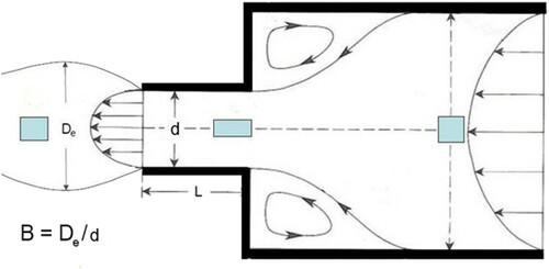
The phenomenon of die swell is very important in processing, especially for extrusion [1]. This is simply described by the degree of extrudate swell of a molten polymer after passing through a die exit, and in the case of a circular die is the ratio of the extrudate diameter to the die diameter, as defined below.

The flow out of the capillary in the form of a continuous meltstream undergoes the phenomenon known as die swell, where the diameter of the meltstream becomes larger than the capillary die diameter. The term generally used to describe the die swell is the swelling ratio, where B = D_e/d. A value of B = 1 will indicate no swelling, B < 1 would indicate contraction out of a die, and B > 1 indicates extrudate swell, which entangled polymers normally show. The die (or extrudate) swell depends upon the shear rate, the L/d ratio and polymer relaxation properties for a given polymer with molecular weight, M_w. The trends found experimentally are that larger extrudate swell was found for shorter L/d ratios, faster shear rates, lower temperatures and higher M_w. The die swell reaches a point at high L/d after which an asymptotic value is obtained. This is due to stress relaxation along the die by the melt.

Die swell has its origins in the entangled nature of polymer chains as we shall explore later in this paper in the discussion. Consequently there is no unique die swell behaviour; it depends upon die geometry, experimental conditions such as temperature, shear rate, and the polymer itself including molecular weight and molecular weight distribution. In addition, when extruding into air at room temperature, rather than an air temperature equivalent to the melt temperature, the true swelling ratio, B, may not be achieved. This may be due to temperature dependence of viscoelasticity, shrinkage from cooling, sagging under gravity (assuming the vertical configuration used by most capillary rheometers), diametral increase due to surface tension effects, and steady flow conditions not being established (see Appendix 4, reference [2] for a full discussion).

The meltstream can also display die exit instabilities, such as irregular oscillatory behaviour in the meltstream, due in part to non-laminar flow (see section 5.10, reference [2]). Under certain circumstances, the flow at the surface will be highly irregular, demonstrating a rough sharkskin appearance, and at higher shear stresses, stick slip phenomena leading eventually to helicoidal defects [1,3]. These behaviours occur at a polymer-specific temperature, shear rate and stress. It is also observed that there is a decrease in swelling with an increase in temperature at a given extrusion rate or shear rate, and that there is a decrease in die swell with an increasing length of the die for a given shear rate. A detailed understanding of this phenomenon is consequently of great practical use for design and production.

In this paper, we will explore the rheological characteristics of two commercial polystyrenes via technological tests melt flow index (or MFI) and by scientific tests (capillary and torsional rheology). The processing behaviour in terms of flow rate and die swell can also be determined from capillary rheology tests as a proxy for die emergent flow in extrusion and from gates in injection moulding. Observations are given regarding flow stability as a function of temperature, shear rate and molecular weight. This is then complemented by torsional rheological measurements presented in the form of ‘master curves’. These master curves are modelled using a rheological fitting function as a function of temperature, and then using contour plotting shown as shear processing maps. This aids practical exploitation of these materials by quickly identifying what effect conditions such as temperature, shear rate and molecular weight have on shear viscosity. An appeal to fundamental polymer physics is made in terms of molecular timescales, and a polymer engineering approximation to this is introduced onto the shear processing maps. Rigorous rheological modelling of such capillary flows confirms this understanding, and reveals the nature of die swell in terms of molecular chain stretch. The likely transition of processing from stable to unstable conditions is related to the molecular timescales inherent in these polymers. Here our aim is to exploit these maps to predict the limits of stable processing rather than to quantify die swell. For this, the timescales identified by detailed molecular theory are sufficient; therefore a simple pragmatic approach is justified.

Melt flow index test

The serendipitous discovery of polyethylene as the result of an industrial accident by ICI in the 1930s [4] necessitated a measure of its flow to characterise batch to batch performance of this new material. This was achieved with the creation of the melt flow index test (or melt volume index) by W. G. Oakes and J. C. Greaves [5]. Owing to the MFI tests inherent simplicity and ease of use, it was used to characterise batch to batch performance of flow in production. This remains the case, but it is also widely reported on single property datasheets for polymers, and has been incorporated into online polymer property databases, such as CAMPUS (Computer Aided Material Preselection by Uniform Standards) [6] since 1988. It is described fully in ISO1133 [7]. It uses a fixed applied load and temperature through a simple capillary rheometer, with a short length to die ratio. The measure of flow from the test (in g/10 min (MFI) or cm³/10 min (MVR)) are not fundamental properties of a polymer.

The die through which the flow is measured has a smooth straight bore 8.000 ± 0.025 mm in length and a diameter of 2.0955 ± 0.0051 mm, thus giving a L:D ratio of approximately 4:1. The details of the test rig and its limitations are described in Appendix 1.

The method has been adopted within standards for individual polymers. In this case, the fixed load and temperatures are adjusted to accommodate the rheological behaviour of the polymers in question so that the apparatus yields a flow result. This means that the MFI test result cannot be used to compare flow behaviour between different classes of polymers (see Appendix 1). Another great limitation of MFI characterisation is that it provides only one set of conditions at which processing is possible, but no further details as to how that process might be optimised under different conditions.

Assuming Hagen–Poiseuille flow in the MFI test, Shenoy et al. [8] converted MFI data into shear viscosity data at set shear rates, allowing for MFI data to be converted to a physical property of use to the technical community. Using this approach, the MFI rig can be used as a simple rheometer. Constructions of approximate viscosity versus shear flow diagrams for a series of different polymers were made.

A more formal analysis of flow for the Melt Flow Rate instrument by Rides et al. [9] gave the following apparent relationships.(1) $\eta ={\displaystyle \frac{300Wg\rho R^4}{{10}^{-3}{D}_{1}L.\mathrm{M}\mathrm{F}\mathrm{I}}}$(1) (2) $\stackrel{.}{\gamma }={\displaystyle \frac{4\left({10}^{-3}\mathrm{M}\mathrm{F}\mathrm{I}/600\rho \right)}{\pi R^3}}$(2) where W = weight in test (kg), g = 9.806 m s⁻², ρ = polymer density at room temperature (MFI), R is radius of the inner die (1.048 mm), D₁ is the inner barrel diameter of the instrument (9.5504 mm), and MFI is the melt flow index, measured in g/10 min.

An example of using these relationships is given in the next section for the materials under consideration in this paper.

Capillary rheometry

High pressure capillary rheometry is an extension of the MFI test device, with an electric drive used to create a series of shear rates at a fixed test temperature [10–13]. The capillary rheometer (first developed for fluids in 1839) predates the MFI rig. The advent of commercial thermoplastics in the late 1930s and 1940s spurred on the development of this type of rheometer as a principal means of measuring shear viscosity [13] at the time.

Typically, the die diameter for the capillary is 1 mm and the length of the capillary can be from 10 to 30 mm, with 20 mm typically chosen, giving an L:D ratio of 20:1. Calculation of the shear viscosity and shear rate data are made with corrections due to Bagley and Weissenberg/Rabinovich, with additional errors in capillary rheometry discussed in Appendix [1] of reference [10]. In addition, errors due to frictional and pressure effects exist using this experimental setup. Thus the resulting data are apparent values for shear viscosity and shear rate only.

The capillary rheometer can also serve as a proxy for an extrusion type process, and consequent observation of the nature of the die swell process is extremely useful in predicting the same in production. In addition to knowing the precise degree of die swell achieved, understanding where the turbulent instability boundaries exist is also useful, since the shear rate just beneath this transition represents an upper bound to processing articles with the necessary smooth finish for consumer use in a given capillary die geometry.

Torsional rheometry

An experimental alternative to the capillary die geometry is to use torsional rheometry, which began in the early 1930s (See Chapter 12, reference [13]).

In this arrangement, a cone and plate or parallel plate geometry can be employed in torsional oscillatory mode at a series of fixed temperatures with varying angular frequencies (see Chapters 3, 8 and 9 of reference [13]). International standards govern its use [14,15]. For polymer melts, there is a preference for parallel plate geometry of a diameter about 25 mm, with a small gap of between 0.5 and 1 mm to contain a polymer sample when dealing with such viscous materials (see pp. 183–184, reference [13]). The resulting data measure the components of elastic or storage (G’) and inelastic or loss modulus (G”) of the complex shear modulus as a function of angular frequency. Employing WLF time-temperature superposition [16] creates rheological master curves, and freely available rheological software (e.g. RepTate [17]) performs this on experimental data to high precision.

From the master curves, the shear viscosity vs. shear rate can be estimated using time-temperature superposition and the Cox–Merz rule [18] by using the following relationship.

The complex viscosity is defined [12] by(3) $\left|\eta \ast \left(\omega \right)\right|={\displaystyle \frac{\sqrt{G^{\mathrm{\prime }}{\left(\omega \right)}^2+G^{\mathrm{\prime }\mathrm{\prime }}{\left(\omega \right)}^2}}{\omega }}$(3) and is calculated from the storage (G’) and loss modulus (G”) as a function of the angular frequency, ω in rad sec⁻¹. The equivalence between $\stackrel{.}{\gamma }$ and $\omega$ from the Cox–Merz rule allows a direct comparison to be made between torsional and capillary rheometry data for simple linear polymers, as we shall demonstrate.

Given torsional rheometry can achieve homogenous shear conditions, it is scientifically preferred to capillary rheometry for precision experimental characterisation of polymer viscosity. In addition it only requires a few grams of sample compared to the other methods mentioned. Nonetheless, both MFI and capillary rheometry continue widely to be used for characterisation of polymer flow. Capillary rheometry is often used as the preferred experimental method for measuring data as input for melt simulation software, such as Moldflow [19]. In this paper we employ all three measures of viscosity and demonstrate the superiority of torsional rheology, by coupling this to die swell observations made in the capillary rheometry tests performed on two commercial polystyrenes.

Phenomenological explanations of die swell

The explanation by Tanner [20] is the most well-known description of extrudate swell, and although is not perfect and has many limitations it can still be useful for predicting extrudate swell. The equation has the form:(4) $B={\left[1+{\displaystyle \frac{1}{2}{\left({\displaystyle \frac{N_1}{2{\tau }_w}}\right)}^2}\right]}^{{\displaystyle \frac{1}{6}}}+1$(4) where N₁ is the first normal stress difference, ${\tau }_w$ is the shear stress at the capillary wall with both terms defined at a particular shear rate, and 0.1 is added to ensure that the extrudate swell tends towards 1.1 in the case of Newtonian fluids. This constant was revised to 0.13 in a subsequent paper [20] using data from computer simulations. Although at first glance B appears to decrease with increasing wall shear stress, N₁ increases more rapidly with ${\tau }_w$, meaning that the overall relationship is an increase in B with ${\tau }_w$. Note there is no explicit dependence upon residence time in the constriction flow channel.

Another simple explanation can be made by referring to Figure 1 and the nature of a fictitious ‘cube’ of polymer displaying rubber like elasticity in the melt state along the centreline of flow through the die. Before the constriction flow begins, we can imagine a ‘cube’ of polymer in a steady state (shown on the right hand side of the diagram). Passing through the constriction flow, and along the die (in the centre of the diagram) results in an elongation in the direction of flow, and a subsequent contraction perpendicular to this flow as the rubbery polymer acts to conserve volume. With the meltstream removed, providing the polymer remains above its glass transition and is still rubbery, the subsequent relaxation causes a recovery towards its initial cuboid shape. This in turn will result in a lateral swelling as the rubbery polymer acts to conserve volume. At a more fundamental level, polymer chains will be undergoing orientation through the constriction flow which will lower their entropy. After emerging from the constriction, the chains will reduce orientation, thus increasing net entropy, causing lateral swelling. This explanation hints that the nature of the constriction flow and residence time would be important, but it lacks the ability to predict behaviour.

Figure 1. Schematic of the die swell phenomenon. Note the apparent flow lines including recirculation zones, and the deformation of a fictitious ‘cube’ of polymer along the centreline of the flow.

A more formal description for extrudate swell was described in terms of elastic deformations [21]. Elastic energy is built up upon squeezing the polymer from the reservoir into the die. The polymer then relaxes to an equilibrium value:(5) ${\displaystyle \frac{W-W_{\mathrm{\infty }}}{W_0-W_{\mathrm{\infty }}}=e^{-kt}}$(5) where W is the elastic energy stored in the material at time t, W_∞ is the energy stored in an infinitely long die and W₀ is the energy stored at t = 0. The elastic energy is then released as an axial expansion and a contraction in the flow direction. This contraction is due to the incompressibility of the polymer melt i.e. that for a fixed volume of polymer the swelling perpendicular to the flow direction must result in a contraction in the flow direction.

These earlier theories work on the assumption that the die is long, i.e. that L/d→∞ and the initial deformation has no effect on the swelling ratio.

Later theories describe extrudate swell as consisting of two parts; a memory of the strain at the die entrance and a shear component describing the flow within the die [22,23]. Short dies, such as those used in practical extrusion have small L/d ratios. This means that the overall residence time in the capillary, ${\tau }_r$, along the flow centre line in the die is short and the polymer has not had time to fully relax in the die.(6) ${\tau }_r={\displaystyle \frac{8\left(L/d\right)}{\stackrel{.}{\gamma }}}$(6) It was experimentally observed [23] for polystyrene that the die swell depended strongly upon L/d, and also upon shear rate $\stackrel{.}{\gamma }$ (hence inversely upon residence time). High shear rates decrease the residence time, thus increasing extrudate swell due to a lack of relaxation. They also increase the shear stress built up within the die, increasing extrudate swell.

Tube theory explanations of die swell

The fundamental relaxation times for a linear response of a polymer using reptation theory [24–26] are related to the equilibration time for a polymer ${\tau }_e$ (defined in Table 7.2 p250 [26]) using the theory of Likhtman and McLeish [25].(7) ${\tau }_d=3{\tau }_e{Z}^3\left(1-{\displaystyle \frac{3.38}{\sqrt{Z}}+{\displaystyle \frac{4.17}{Z}+{\displaystyle \frac{1.55}{Z^{3/2}}}}}\right)$(7) (8) ${\tau }_R={\tau }_e{Z}^2$(8)

Z is the number of chain entanglements (Z = M_w/M_e, where M_e is the entanglement molecular weight [26]).

The equilibration time is the Rouse reorientation time required to relax a piece of the chain just enough to occupy a single tube segment [26], and is normally a very short time (observed at fast rates during processing, since time and rate are inversely related).

The relaxation times for a linear polymer are the reptation (disengagement) time ${\tau }_d$ and the Rouse (reorientation) time ${\tau }_R.$ These are formally defined in Table 7.2 p250 [26] respectively.

At very long timescales or low shear rates, the polymer is relaxed and reaches its highest shear viscosity (zero shear). Above a critical molecular weight, the zero shear viscosity for linear polymers at a given temperature follows the form ${\eta }_o\approx M_w^{3\cdot 4}$, thus following the number of chain entanglements raised to the power 3.4.

The reptation (disengagement) Weissenberg number is defined by$W_d={\dot{\gamma }}_w\times {\tau }_d$with${\dot{\gamma }}_w$ the apparent (Newtonian) wall shear rate from experiment and ${\tau }_d$ is the reptation (disengagement) time of the polymer. Similarly the Rouse–Weissenberg number is defined by $W_R={\dot{\gamma }}_w\times {\tau }_R$, with ${\dot{\gamma }}_w$ the apparent (Newtonian) wall shear rate from experiment and ${\tau }_R$ is the Rouse reorientation time of the polymer. The reptation (disengagement) time ${\tau }_d$ is the time at which chain orientation starts to become a significant factor, and marks the onset of a sharp fall in shear viscosity and the transition from viscoelastic to elastic flow. The Rouse (reorientation) time ${\tau }_R$ indicates the time at which chain stretching starts to become a significant factor. The polymer will have shear thinned significantly from its zero shear value, and the melt will show increasing elastic behaviour. Given that processing at rates with $W_R$ > 1 will result in both chain orientation and stretching more defects due to elastic recovery of the extrudate would be expected.

We have demonstrated for polystyrene [27–29] that die swell behaviour scales with the Rouse–Weissenberg number for a series of different molecular weights and polydispersities at the same test temperature of 180°C using a Multipass Rheometer (MPR) operating with a temperature and nitrogen controlled environment. The MPR consists of two hydraulically driven pistons, each inserted into a barrel filled with polymer. In between the upper and lower barrels is a specially designed test section into which a variety of testpieces can be inserted. Quartz viewing windows inserted into the test section allowed visualisation of the flow during the test. The MPR can perform experiments using as little as 10 g of polymer and has been adapted for contraction-expansion, extrusion, capillary and cross slot flows. In our work [28,29], we used the MPR in a novel mode in which the lower chamber was empty, enabling controlled visualisation of isothermal extrusion.

This was supported by a constitutive model for the polymers consistent with tube theory, such as the Rolie–Poly (Rouse linear entangled polymer) equation of monodisperse entangled linear polymer melts [30]. Fitting torsional rheology data to the models was provided by using the RepTate software [17]. The parameters generated by RepTate were used within the Lagrangian finite element solver flowSolve [31] for flow modelling and computation of the shearing and extensional flows encountered in extrusion flow. A single stretching mode version of the Rolie-Poly equation was used to simulate monodisperse melts and the multi-mode Rolie–Double–Poly equation [32] was used for simulation of bidisperse and polydisperse melts. A modified version was used to include finite extensibility for the single stretching Rolie–Poly element of monodisperse melts and the two stretching elements used in models of the bidisperse melt [27–29]. Experimentally we demonstrated that the isothermal die swell for polystyrenes with molecular weights in the range of 100–400 kDa showed the behaviour reported in literature. For each polymer, at low Newtonian shear wall rates the die swell was small (about 1.1), then climbed up to values in the range 1.8 to 2.1. The amount of die swell for a given Newtonian shear wall rate depended upon molecular weight, with higher Mw resulting in higher die swell. It was found that the die swell behaviour at all molecular weights collapsed on to a single curve when the Rouse–Weissenberg number was used to plot the data instead of the measured Newtonian wall shear rate. For $W_R<7$ simulations using the flowSolve programme agreed with the experimental data. For $W_R\ge 7$ the MPR show a reduction in the gradient of the increase in extrudate swell with shear rate, relative to the theoretical predictions.

In our previous work it was not possible to experimentally demonstrate that prediction of die swell was thermorheologically simple. Here, we rigorously examine die swell in non-isothermal extrusion. Combining linear rheology to identify key molecular relaxation timescales with temperature and shear dependence of viscosity from capillary rheology, we demonstrate that die swell can be fully predictable over a wide range of temperature and processing conditions without recourse to the most complex molecular theories. The method of plotting molecular timescales as shear viscosity maps is designed to provide more useful insights to flow behaviour than MFI measurements, by showing the magnitude of shear viscosity when contour plotted against temperature and shear rate, and also predicting the magnitude of extrudate swell and the onset of flow instabilities during processing.

Materials and methods

Materials

Commercial Polystyrene samples were purchased from Sigma Aldrich, with the codes PS192 (product number 430102) and PS350 (product number 441147). These have nominal molecular weights of 192 and 350 kDa respectively and their full molecular weight distributions were experimentally measured using GPC and rheological techniques.

GPC

A gel permeation chromatography (GPC) characterisation was performed on both polystyrene samples. The samples were all run using THF as the solvent at 35°C. The instrument was a Viscotek TDA 302 instrument with a triple detector system.

Rheological characterisation

MFI

A Rosand MFI grader based at Intertek, Wilton, was used with the geometry defined in section ‘Melt flow index test’. A test temperature of 200°C and applied weight of 5 kgf were employed. Samples were cut after 10 min and weighed to determine the melt flow index, expressed in g/10 min.

Capillary rheometry

A Rosand RH7 capillary rheometer located at Intertek, Wilton, was used. A 1 mm diameter, 20 mm length extruder was used. Shear rates in the region of 30–30,000 s⁻¹ were used at four temperatures; 160°C, 175°C, 190°C and 220°C. Each shear rate was calculated with a Rabinowitsch correction applied to account for the non-Newtonian nature of the material. This uses a plot of log shear rate vs. shear stress to calculate a correction factor, n, for the polymer. Video images of the extrudate were acquired for all speeds using a standard digital camera operating at 30 frames per second. B values were obtained by measuring the diameter of the extrudate with a set of calipers once cooled. Multiple measurements were taken along the length of the extrudate and an average value taken to obtain a B value. During capillary measurements all shear rates were done in a continuous experiment consisting of discrete shear rates. At each shear rate for each temperature, the extrudate was cut at the die exit so as to eliminate the effect of gravity and the diameter measured at room temperature by vernier digital calipers at 5 or more points down the solid sample to determine the swelling ratios.

Torsional rheometry

Polymer chip samples were compression moulded into discs of 25 mm diameter and approximately 1 mm thickness at 160°C, before cooling to room temperature. The disc samples were placed in an oven at 80°C before testing, to ensure they were thoroughly dried.

The rheological behaviour of both polymers was measured using oscillatory rheological methods, described in detail by Mezger [13]. The measurements were performed using a TA AR2000 rheometer using 25-mm parallel plate geometry, under a nitrogen atmosphere. The discs were squeezed between the parallel plates under atmospheric pressure until a gap of approximately 1-mm thickness and a small normal force was registered by the rheometer. To determine the full rheological response, oscillatory tests were performed at angular frequencies between 0.1 and 100 rad s⁻¹ with five intervals per decade, and with strain amplitudes of 1%, after examination of the dynamic strain sweep as a function of frequency and temperature.

Test temperatures were in the range between 125°C and 230°C in 15°C interval steps. Time-temperature superposition of the data was performed using the RepTate software system [17], according to the methods outlined by Ferry [16].

Results

GPC

Following the method shown in Appendix 2, the data according to the GEx distribution for the polymers is as follows (Figure 2).

Figure 2. Molecular weight distribution data for the PS192 (red) & PS350 (blue) samples. The triangles indicate the position of the weight average molecular weights, M_w, for each sample as per Table 1.

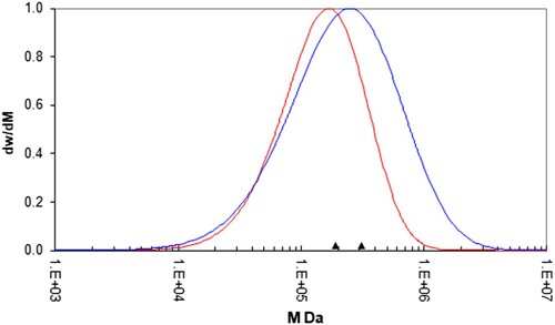
Table 1. Average molecular weight distribution data for all polymers used.

Polymer	Mw/kDa	Mn/kDa	Dispersity
PS350	350	116	3.01
PS192	192	100	1.92

MFI

These data can be converted to give approximate values for the shear viscosity and shear rate using Equations (1) and (2) (Table 2).

Table 2. Mean MFI data (with the standard deviation given in brackets) for both polymers.

Polymer	MFI g/10 min @200°C & 5 Kgf
PS350	2.07 (0.02)
PS192	9.63 (0.12)

These are plotted in Figures 3 and 4.

Figure 3. Apparent shear viscosity vs. apparent wall shear rate, together with the calculated value from the MFI test at the indicated test temperatures (°C) for the PS192 sample.

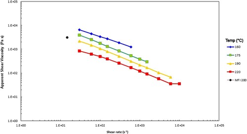
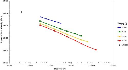
Figure 4. Apparent shear viscosity vs. apparent wall shear rate, together with the calculated value from the MFI test at the indicated test temperatures (°C) for the PS350 sample.

Capillary rheology

The apparent shear viscosities measured by capillary rheometer are plotted vs. apparent wall shear rates, together with the calculated values from the MFI test reported in Table 3.

Table 3. Apparent shear viscosity and wall shear rates derived from MFI data at 200°C.

Polymer	Apparent shear viscosity Pa.s	Apparent shear rate s^−1
PS350	1.23 × 10^4	3.7
PS192	3.00 × 10^3	15.0

The MFI and capillary rheology test data are broadly consistent, but the shear viscosity calculated from the MFI test is a bit high, perhaps because the rates in the test lack the effects of shear thinning that are likely to be greater for capillary rheology, especially with a high molecular weight tail in the distribution.

The die swell values from each sample are shown in Figures 5 and 6.

Figure 5. Die swell at the indicated test temperatures (°C) for the PS192 samples. The error bars give the ± 95% range calculated from the standard deviation from the test.

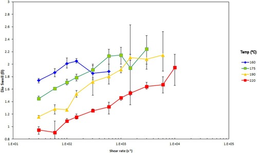
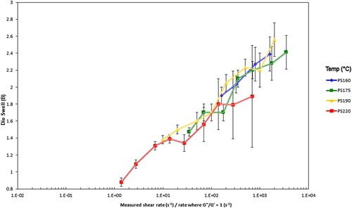
Figure 6. Die swell at the indicated test temperatures (°C) for the PS350 samples. The error bars give the ± 95% range calculated from the standard deviation from the test.

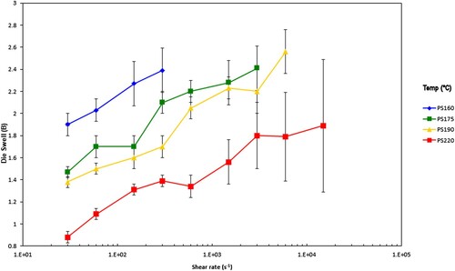
As expected, for both samples the die swell increases with increasing shear rate and falls with increasing test temperature. Beyond a certain shear rate the behaviour of the extrudate transitions from steady state flow to unstable. This tends to be at lower shear rates when the temperatures are low, and higher shear rates when the temperatures are high for both polymers.

Torsional rheology

The data were measured at the time and shear rate intervals indicated in the section ‘Torsional rheometry’ and were then time-temperature shifted to produce master curves of the complex shear viscosity (Pa.s) and the storage (G’) and loss (G”) modulus (Pa) as a function of frequency (rad s⁻¹), shown below at 200°C (Figure 7 and 8).

Figure 7. Complex shear viscosity (marked as triangles), storage (G’ marked as circles) and loss (G” marked as diamonds) modulus vs. frequency (rad s⁻¹) shifted to 200°C for the PS192 sample. The first cross over frequency (where G’ = G”) occurs at 1.72 × 10² rad s⁻¹, and the second cross over frequency (where G’ = G”) occurs at 4.29 × 10⁴ rad s⁻¹.

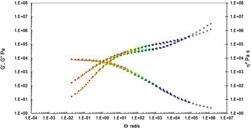
Figure 8. Complex shear viscosity (marked as triangles), storage (G’ marked as circles) and loss (G” marked as diamonds) modulus vs. frequency (rad s⁻¹) shifted to 200°C for the PS350 sample. Note the first cross over frequency (where G’ = G”) occurs at 3.19 × 10⁰ rad s⁻¹, and the second cross over frequency (where G’ = G”) occurs at 3.97 × 10⁴ rad s⁻¹.

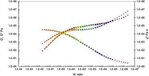
For both polymers the complex shear viscosity was calculated using Equation (3) from the storage (G’) and loss modulus (G”) as a function of the angular frequency, ω, in rad sec⁻¹.

Discussion

The single point MFI values suggest that the values suggest that the lower M_w PS192 will have a lower viscosity than PS350 in the limit of low shear rate. The converted shear viscosity and shear rate data given in Table 3 confirms this. These single point data offer no guidance of the rheological behaviour with changes in temperature or shear rate.

The capillary data presented in Figures 3 and 4 for both polymers suggest that as expected raising the temperature and shear rate causes the shear viscosity to fall. Note the single point MFI data converted to shear viscosity and shear rate are also plotted in these Figures and look slightly higher than expected from the capillary data. The die swell data presented in Figures 5 and 6 for both polymers suggest that as expected decreasing the temperature and increasing the shear rate causes the die swell to increase, consistent with other literature on similar systems [21–23]. PS350 shows higher die swell compared to PS192. The positions of transition from stable to unstable extruded lace vary as described earlier. At lower temperatures this transition occurs at a lower shear rate.

The capillary rheology data offer no obvious explanation for the degree of die swell, as traditionally the experimentalist must also measure the first normal stress difference usually only obtainable from torsional rheometry and follow Tanner’s method outlined in the section ‘Phenomenological explanations of die swell’.

In our previous publications [27–29], we have employed simulation to demonstrate the origin of die swell as a chain phenomenon using contemporary polymer physics [30]. The experiments in this case were conducted under isothermal conditions and in contrast the following method can be used as guidance for melt processors operating under more commercial conditions, where die swell occurs under non-isothermal conditions. Taking the torsional rheological data and performing time-temperature shifts (TTS) via the Reptate software package produces a series of shear viscosity vs. shear rate curves at different temperatures. The values for the TTS parameters are shown in Table 4 and the viscosity curves are shown in Figures 9 and 10.

Figure 9. Complex shear viscosity (marked as circles) vs. frequency at the indicated temperatures after performing time-temperature superposition for PS192. The data with lines has been interpolated using the methods described below at the temperatures indicated using Equation (10). The dashed line corresponds to the complex shear viscosity shown in Figure 7.

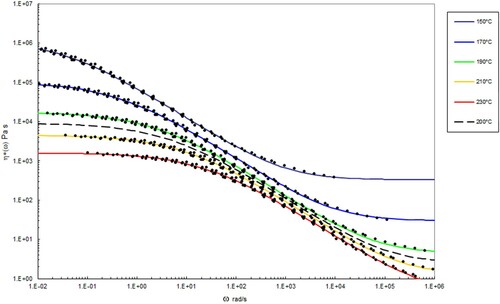
Figure 10. Complex shear viscosity (marked as circles) vs. frequency at the indicated temperatures after performing time-temperature superposition for PS350. The data with lines has been interpolated using the methods described below at the temperatures indicated using Equation (10). The dashed line corresponds to the complex shear viscosity shown in Figure 8.

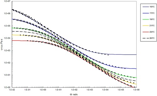
Table 4. WLF parameters used for time-temperature shifts to the torsional rheology at a shift temperature of 200°C.

Polymer	C1	C2	ρ0	C3
PS192	4.188	−52.114	0.95	0.69
PS350	4.324	−50.480	0.95	0.69

For each polymer the shear viscosity vs. shear rate data were fitted at five temperatures (150°C to 230°C in 20°C intervals) using the Carreau/Yasuda equation [12].(10) $\eta \left(\stackrel{.}{\gamma }\right)={\eta }_{\mathrm{\infty }}+\left({\eta }_0-{\eta }_{\mathrm{\infty }}\right){\left[1+{\left(\lambda \stackrel{.}{\gamma }\right)}^{P1}\right]}^{{\displaystyle \frac{P-1}{P1}}}$(10) where η₀ is the zero shear viscosity; η_∞ is the infinite shear viscosity; λ is a term described as the ‘relaxation time’; P1 and P are terms associated with the power law behaviour of the fluid, governing its shear thinning behaviour, typically in the range zero to 1; Only η₀, the zero shear viscosity has physical meaning; the rest of the terms are fit to the data.

In Figures 9 and 10, the best fit to the data at each temperature using the Carreau/Yasuda equation is shown by the lines in the various colours. The dashed line shows the interpolated behaviour at 200°C using the following method.

By setting P1 and P to constant values and allowing only η_∞, η_o and λ to vary as a function of temperature, the following table can be constructed for the parameters in the Carreau/Yasuda equation as a function of temperature (Tables 5 and 6).

Table 5. Parameters used to model the rheology of PS192 by the Carreau/Yasuda equation as a function of temperature.

	230°C	210°C	190°C	170°C	150°C
η∞	5.00 × 10^−^1	1.50 × 10^0	5.00 × 10^0	3.00 × 10^1	3.20 × 10^2
η0	2.00 × 10^3	5.00 × 10^3	1.70 × 10^4	1.00 × 10^5	1.50 × 10^6
λ	5.20 × 10^−2	1.26 × 10^−1	3.98 × 10^−1	1.58 × 10^0	3.10 × 10^1
P1	0.48	0.48	0.48	0.48	0.48
P	0.20	0.20	0.20	0.20	0.20

Table 6. Parameters determined to model the rheology of PS350 by the Carreau/Yasuda equation as a function of temperature.

	230°C	210°C	190°C	170°C	150°C
η∞	4.50 × 10^-1	1.30 × 10^0	5.50 × 10^0	3.20 × 10^1	4.50 × 10^2
η0	6.35 × 10^3	1.84 × 10^4	7.18 × 10^4	4.40 × 10^5	5.54 × 10^6
λ	2.09 × 10^-2	5.92 × 10^-1	2.26 × 10^0	1.35 × 10^0	1.64 × 10^2
P1	0.73	0.73	0.73	0.73	0.73
P	0.21	0.21	0.21	0.21	0.21

The parameters η_∞, η_o and λ vary with temperature in a systematic way. Plotting the logarithm of these parameters versus temperature allows them to be fitted by a hyperbolic function of the form y = a + b/T (Figures 11 and 12).

Figure 11. Values for log η_∞, log η₀, log λ as a function of temperature, The fitted curves show the best fit obtained with the hyperbolic function, log η_∞, log η₀, log λ = a + b/T for PS192.

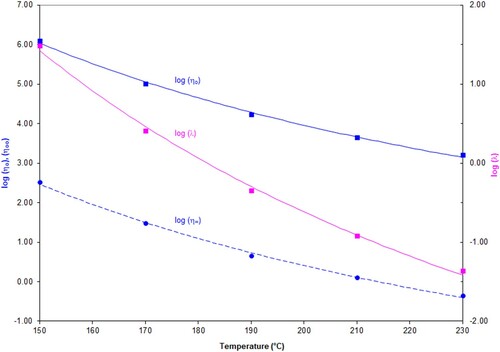
Figure 12. Values for log η_∞, log η₀, log λ as a function of temperature, The fitted curves show the best fit obtained with the hyperbolic function, log η_∞, log η₀, log λ = a + b/T for PS350.

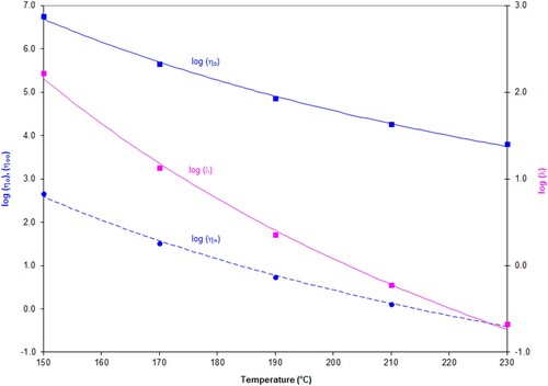
Parameters a, b to fit the hyperbolic function, log η₀, log η_∞, log λ = a + b/T can be determined for each polymer.

The values for a and b are shown in the two tables below.

The equilibration time for a polymer ${\tau }_e$ at temperature T scales to the value for ${\tau }_e$ at a reference temperature (in this experiment 200°C), hence ${\tau }_{e200}$.(11) ${\tau }_e=\frac{{\tau }_{e200}}{{10}^{\left[-C_1\left(\frac{200+C_2}{T+C_2}\right)\left(\frac{200-T}{200+C_2}\right)\right]}}$(11) The first and second crossover timescales also follow this type of relationship.

The molecular timescales ${\tau }_R,$ and ${\tau }_d$ described by Equations (7) follow time-temperature superposition according to the WLF shift in [16].(12) ${\tau }_R={\displaystyle \frac{{\tau }_{e200}}{{10}^{\left[-C_1\left(\frac{200+C_2}{T+C_2}\right)\left(\frac{200-T}{200+C_2}\right)\right]}}{\left({\displaystyle \frac{M}{M_e}}\right)}^2}$(12) (13) $\begin{array}{rl}{\tau }_d& =\frac{{\tau }_{e200}}{{10}^{\left[-C_1\left(\left(200+C_2\right)/\left(T+C_2\right)\right)\left(\left(200-T\right)/\left(200+C_2\right)\right)\right]}}{\left(\frac{M}{M_e}\right)}^3\\ & \times \left(1-\frac{3.38}{\sqrt{Z}}+\frac{4.17}{Z}+\frac{1.55}{Z^{3/2}}\right)\end{array}$(13)

A shear viscosity ‘map’ for each polymer vs. temperature (°C) and shear rate (s⁻¹) can be produced by combining Equation (10) with the parameters in Tables 7 and 8 via contour plotting software. In addition, the molecular timescales as a function of temperature can be replotted from Equations (11)–(13), converting these to rates. These are shown in Figures 13 and 14.

Figure 13. Shear viscosity map for PS192.

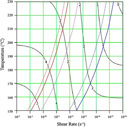
Figure 14. Shear viscosity map for PS350.

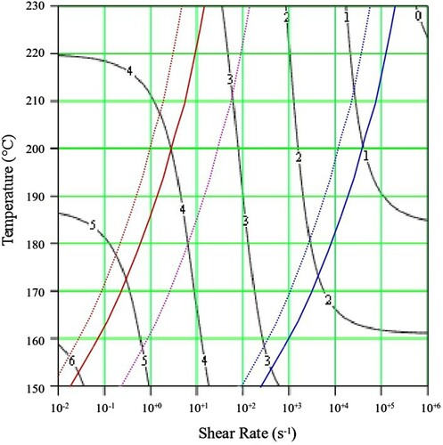
Table 7. Values for PS192 for parameters which vary according to log η₀, log η_∞, log λ = a + b/T, where T is the test temperature in °C.

	a =	b =
log (η∞)	−7.473	1559.098
log (η0)	−3.046	1497.850
log (λ)	−7.975	1482.677

Table 8. Values for PS350 for parameters which vary according to log η₀, log η_∞, log λ = a + b/T, where T is the test temperature in °C.

	a =	b =
log (η∞)	−6.020	1291.385
log (η0)	−1.767	1268.346
log (λ)	−6.165	1248.631

The contours in black show the value of the log₁₀ viscosity in Pa.s. In addition, lines are drawn which indicate where molecular timescales for each polymer are calculated from the weight average number of entanglements per chain, Z. These are marked by the red dotted line (reptation time ${\tau }_d$), purple dotted line (Rouse (reorientation) time ${\tau }_R$ and blue dotted line (equilibration time ${\tau }_e$). Determined experimentally, the solid red line shows the first cross over frequency (where G’ = G”; an approximate polymer engineering view of the reptation time, ${\tau }_d$, without recourse to theory). Also shown is the solid blue line which marks the position of the second cross over frequency (where again G’ = G”). The interpolated shear viscosity by the Carreau/Yasuda equation is reliable for up to a decade beyond the blue line (as seen from the data in Figures 7 and 8).

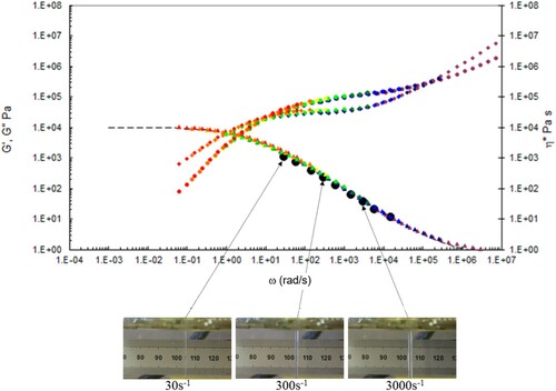
In Figures 15–22, we show the capillary rheology data, together with the time-temperature shifted torsional rheology data at the test temperatures indicated, also plotted are the Carreau/Yasuda equation predictions, together with the observed die swell behaviour at low, intermediate and high shear rates. The data are marked by capillary (black dots) and torsional rheology data (small dots). Also shown are the complex shear viscosity (marked as triangles), storage (G’ marked as circles) and inelastic (G” marked as diamonds) moduli vs. frequency (rad s⁻¹), and finally the Carreau/Yasuda equation by the dotted line at each temperature.

Figure 15. Combined capillary (black dots) and torsional rheology data (small dots) for PS192 at 160°C.

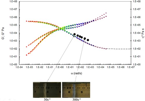
Figure 16. Combined capillary (black dots) and torsional rheology data (small dots) for PS192 at 175°C.

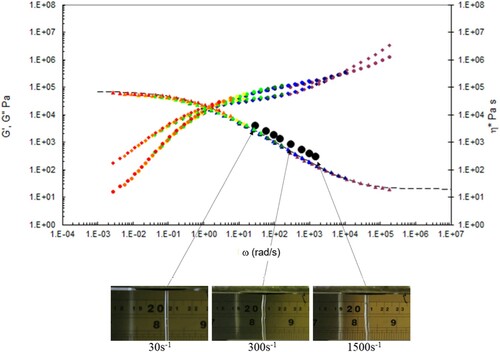
Figure 17. Combined capillary (black dots) and torsional rheology data (small dots) for PS192 at 190°C.

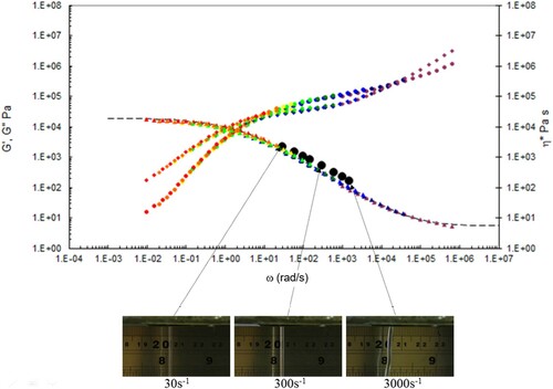
Figure 18. Combined capillary (black dots) and torsional rheology data (small dots) for PS192 at 220°C.

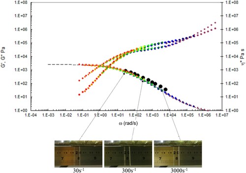
Figure 19. Combined capillary (black dots) and torsional rheology data (small dots) for PS350 at 160°C.

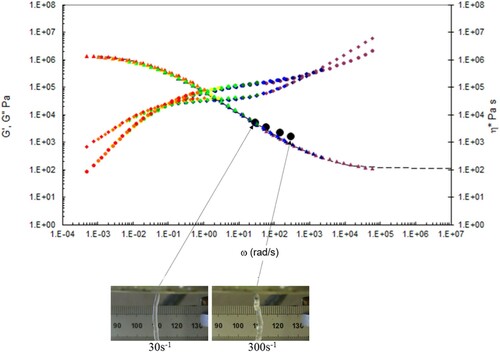
Figure 20. Combined capillary (black dots) and torsional rheology data (small dots) for PS350 at 175°C.

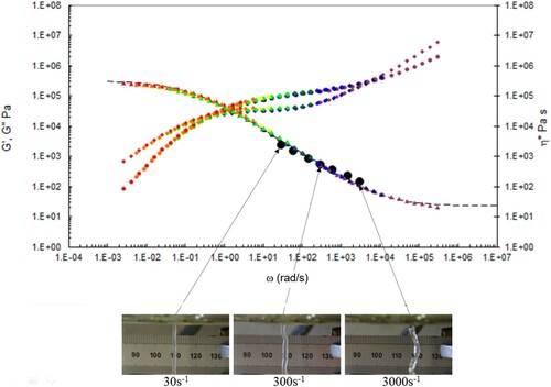
Figure 21. Combined capillary (black dots) and torsional rheology data (small dots) for PS350 at 190°C.

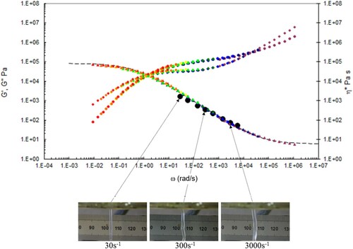
Figure 22. Combined capillary (black dots) and torsional rheology data (small dots) for PS350 at 220°C.

A number of observations can be made from the data in Figures 15–22.

1. There is good agreement between the capillary and torsional viscosity data for both polymers, especially at higher temperatures.

2. The Carreau/Yasuda equation shown by the dotted lines and interpolated at the test temperatures shows excellent agreement with the torsional viscosity data. This gives confidence that the shear viscosity maps represent a good picture across the experimental space of temperature and shear rates shown in Figures 13 and 14. To show the utility of the maps, note that for PS350 at 220°C, at low shear rates the contour value of the log₁₀ viscosity in Pa.s in Figure 14 is about 4 (=10,000 Pa.s). Referring to the experimental data for PS350 at 220°C in Figure 22 indicates this is so, and consequently the method is reliable. The Carreau/Yasuda equation interpolation method can be used to produce detailed isothermal predictions for shear viscosity as a function of shear rate, assuming the assuming the Cox–Merz rule applies to the complex viscosity derived using Equation (3), which is useful for flow design calculations.

3. The die swell behaviour shows the familiar pattern of increasing die swell as the temperature falls, and the shear rate increases for both polymers. More subtly, there appears to be a transition for the extruded lace from stable to unstable (becoming ‘wibbly-wobbly’) as the temperature falls, and the shear rate increases.

The explanation for the latter behaviour lies in our earlier papers [27–29] where we demonstrated that die swell is a phenomenon associated with the Rouse–Weissenberg number, defined by $W_R={\dot{\gamma }}_w\times {\tau }_R$, with ${\dot{\gamma }}_w$ the apparent (Newtonian) wall shear rate from experiment and ${\tau }_R$ the Rouse reorientation time of the polymer. We apply the same technique to the data in Figures 5 and 6, scaling the data by W_R. The timescales used for this scaling are shown in Table 9 and the scaled data are shown in Figure 23.

Figure 23. Die swell for the PS192 samples vs. Rouse–Weissenberg number. The error bars give the ± 95% range calculated from the standard deviation from the test.

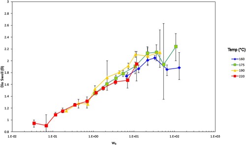
Table 9. Timescales in seconds for the two polymers in the study. These are for the reptation (disengagement) time ${\tau }_d$, first cross over frequency (where G; = G”), Rouse (reorientation) time ${\tau }_R$, second cross over frequency (where G’ = G”), and finally ${\tau }_e,$ the equilibration time all determined at 200°C. The cross over frequency times were identified experimentally from Figures 10 and 11.

	First			Second
	${\tau }_d$ (s)	G’ = G” (s)	${\tau }_R$ (s)	G’ = G” (s)	${\tau }_e$ (s)
PS192	1.21 × 10^-1	5.82 × 10^-2	1.06 × 10^-2	2.33 × 10^-5	7.84 × 10^-5
PS350	9.99 × 10^-1	3.13 × 10^-1	3.52 × 10^-2	2.52 × 10^-5	7.84 × 10^-5

Recall the data presented earlier in Figures 5 and 6, where the die swell for each polymer was shown at the test temperatures. At 200°C, the molecular timescales shown in Table 9 were calculated.

Consistent with theory, ${\tau }_e$ is independent of molecular weight, but ${\tau }_R$ and ${\tau }_d$ scale with molecular weight according to Equations (7) and (8) (Figure 24).

Figure 24. Die swell for the PS350 samples vs. Rouse–Weissenberg number. The error bars give the ± 95% range calculated from the standard deviation from the test.

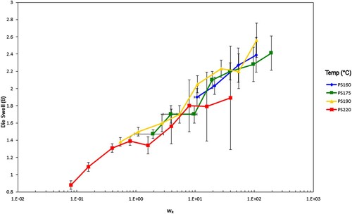
These figures show a lack of temperature dependence because of the decrease in relaxation times with increasing temperature. This is to be expected as the relaxation times of the material decrease with increasing temperature, as seen from the shear viscosity map. The higher molecular weight sample, PS350, has the higher extrudate swell. The effect is slight, partially due to polydispersity smoothing out the differences between the polymers since at an identical shear rate the extrudate swell is higher. At the highest shear rates the swelling ratios fall significantly where gross melt fracture has occurred, partly due to gravitational effects from the test. This shows the superposition versus Rouse–Weissenberg number up to the limit of melt fracture. This reinforces the ability to not only shift extrudate swell by molecular weight, but also TTS shift it, even during non-isothermal extrusion.

A simple method can also be employed without recourse to fundamental theory, by assuming that the first cross over frequency (where G’ = G”) is an approximate polymer engineering view of the reptation time, ${\tau }_d$. Simply by taking the measured shear rate from the experiment and dividing it by the shear rate for the first cross over frequency (where G’ = G”) produces an ‘experimental’ Weissenberg number, as can be seen in Figures 25 and 26.

Figure 25. Die swell for the PS192 samples vs. experimental Weissenberg number (ratio of measured shear rate to rate where G’ = G”). The error bars give the ± 95% range from the standard deviation from the test.

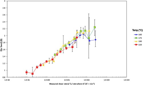
Figure 26. Die swell for the PS350 samples vs. experimental Weissenberg number (ratio of measured shear rate to rate where G’ = G”). The error bars give the ± 95% range from the standard deviation from the test.

The superposition of die swell with temperature for any given molecular weight distribution is the same as the formal Rouse–Weissenberg number approach, seen in Figures 23 and 24, but does not require the theory.

By marking where the molecular transitions and the experimentally determined Weissenberg number (ratio of measured shear rate to rate where G’ = G”) together with the shear viscosity as a function of shear rate on the shear viscosity maps one can predict both the amount of flow and its nature in this experiment.

When processing at rates faster than W_R = 1 the die swell will significantly increase. Experimentally, when processing at rates about a decade faster than the first cross over frequency (where G’ = G”), we again get significant die swell. The nature of this as we demonstrated is the onset of chain orientation and stretching resulting in more elastic behaviour from the melt. Turbulence is a Rouse-time linked phenomenon and the turbulence occurs approximately above W_R = 5. Alternatively, at rates greater than a decade faster than the first cross over frequency, the extruded lace becomes turbulent in nature, corresponding to the formal W_R = 5 criteria.

It appears to be nothing to do with viscosity. This can be seen in Figure 27 for PS350 and in the following video link [33]. The shear viscosties are very close, but the die swell amount and nature (stable vs. unstable) are quite different. Referring to the shear viscosity map for PS350 in Figure 14 shows why this is so. The contours of shear viscosity at 190°C and 220°C in the diagrams are between 2 and 3 and fall away at the same rate with increasing shear rate, thus ensuring similar shear viscosities. At 220°C, the experimental point is just above the Rouse (reorientation) time ${\tau }_R$, indicating a low Rouse–Weissenberg number and stable extruded lace. However at 190°C, the experimental point is below the time, or above the rate, implying that chain stretch cannot fully, with more die swell and unstable extruded lace.

Figure 27. Die swell for the PS350 samples at 190°C & 600 s⁻¹ (left-hand side) & 220°C & 300 s⁻¹ (right-hand side). Videos of these extrusion experiments are discussed in detail elsewhere [33].

Careful comparison of the shape and nature of the die swollen extruded lace at the test temperatures and rates indicated in Figures 15–22 makes sense for all conditions and materials when related to the shear viscosity maps for each polymer. Instability in the extruded lace occurs exclusively when the shear rate exceeds $\left(1/{\tau }_R\right)$, and stable flow is always found at lower extrusion rates.

From the flow maps it is also possible to calculate the maximum molecular weight of polymer that could be processed at a particular shear rate, and to estimate the shift in temperature required to accommodate a change in molecular weight for a defined process rate. We note that for PS350 at 220°C the zero shear viscosity is approximately 10⁴ Pa.s (marked as 4 when plotted as the contour logarithm on Figure 16), and also that the Rouse (reorientation) time ${\tau }_R$, has a value of approximately 10² s⁻¹. On the shear viscosity map of PS192 in Figure 13, at 200°C the zero shear viscosity is approximately 10⁴ Pa.s, and the Rouse (reorientation) time ${\tau }_R$, also has a value of approximately 10² s⁻¹. The timescale observation can be shown in more detail by plotting the results of Equations (15)–(17)] as a function of molecular weight for polystyrene, assuming M_e = 16.5 kDa (Figures 28 and 29).

Figure 28. Molecular timescales for polystyrene assuming the WLF constants reported in Table 4, with M_e = 16.5 kDa at 203.1°C. The red line shows the position for the reptation time, ${\tau }_d$, the green line shows the position for the Rouse (reorientation) time ${\tau }_R$, and the blue line for the equilibration time ${\tau }_e$. The dotted line shows that ${\tau }_R$ = 10⁻² s at 192k Mw.

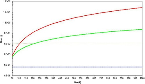
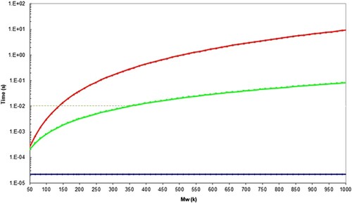
Figure 29. Molecular timescales for polystyrene assuming the WLF constants reported in Table 4, with M_e = 16.5 kDa at 222.3°C. The red line shows the position for the reptation time, ${\tau }_d$, the green line shows the position for the Rouse (reorientation) time ${\tau }_R$, and the blue line for the equilibration time ${\tau }_e$. The dotted line shows that ${\tau }_R$ = 10⁻² s at 350k Mw.

By comparison of viscosities, this implies their flow would be similar at low to intermediate shear rates. Looking at the master curves Figure 7 for PS192 and Figure 22 for PS350 suggests this is so. In this sense the change in molecular weight between the two polymers results in a rheology that can be offset by a processor by adjusting the temperature by approximately 20°C to get a similar response. The master curves for the two polymers in Figures 7 & 22, and the shear viscosity maps in Figures 13 and 14 support this.

Conclusions

In this paper we have shown that torsional rheology, supported with TTS and the Carreau/Yasuda equation enables the full range of processing conditions for a given material to be optimised, based on a series of non-destructive tests applied to a single, gram-scale sample using torsional rheological measurements. The melt flow index (MFI) and capillary rheology tests require considerably more material to conduct the test. The MFI test shows limited usefulness, indicating that a lower molecular weight achieves more flow than a higher molecular weight as expected. The capillary tests generated shear viscosity vs. shear rate at a series of temperatures which can be used for design purposes. In addition, measurements of extrudate swell B values were obtained, showing a pattern of increasing die swell at W_R > 1 with increasing shear rate and reduced temperature. The melt lace made a transition from stable to unstable behaviour at a range of shear rates for both polymers as a function of temperature. Torsional linear rheology allows the generation of a master curve, with the determination of molecular timescales linked to reptation theory. Shear viscosity maps vs. temperature and shear rate, plotted as logarithmic contours of shear viscosity were created. The MFI tests represent a single point in these maps. The capillary rheology data are made at constant temperature slices across the map. The torsional rheology data when employed in the form of the shear viscosity map covers the whole experimental space to high precision. This allows a designer to quickly ascertain rheological behaviour across a wide range of experimental conditions. Superimposing upon this map the positions Rouse and reptation times as a function of temperature allows a qualitative assessment of the degree of chain orientation and stretching in the melt. The B values superimpose onto a single line when plotted using the Rouse–Weissenberg number. Alternatively using an empirical measure for the onset of chain orientation and stretching (the first cross over frequency where G’ = G”) also results in the die swell collapsing onto a single line when the experimental shear rate is normalised by the first cross-over frequency. This method does not require knowledge or use of advanced theory. The full shear viscosity map, together with the polymer timescales thus serves as a powerful design tool to predict rheological behaviour.

Acknowledgements

The authors would like to thank Professor Tom McLeish for many conversations and useful guidance, and Jon Millican for characterising the polymers by GPC.

Disclosure statement

No potential conflict of interest was reported by the authors.

Additional information

Funding

This work was supported by the Engineering and Physical Sciences Research Council CDT in Soft Matter and Functional Interfaces (SOFI), Grant Ref. No. EP/L015536/1.

Appendixes

Appendix 1. Melt flow index

A schematic of the test is shown below.

Figure A1. Schematic of the MFI test apparatus.

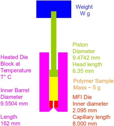
A polymer mass is introduced into the inner barrel and heated until uniformly melted. A fixed weight is then applied, and the molten polymer flows through the exit die, with an L:d ratio of 4:1. The measure of flow from the test is measured in g/10 min (MFI) or cm³/10 min (MVR).

Note there is no commonality of test conditions; these are adjusted for each type of polymer so that the rig can make a measurement given the difference between the rheological behaviour of polymers, as Figure (A1.2) shows.

Figure A2. Range of temperatures and loads used in the MFI/MFR test by generic polymer, as suggested in section 8 of ASTM D1238 [34].

In this sense, the MFI test cannot be used to compare the flow behaviour of polymers; it indicates likely temperatures and forces that would make a polymer flow through the rig, but no further details as to how that process might be optimised.

Appendix 2. Generalised exponential function approximation to molecular weight

The Generalised Exponential Function (GEx) when applied to molecular weight distributions [35,36] has the form(A1) $W_{GEx}\left(a,b,M_o,M\right)={\displaystyle \frac{b}{M_o.\mathrm{\Gamma }\left({\displaystyle \frac{a+1}{b}}\right)}{\left({\displaystyle \frac{M}{M_o}}\right)}^a.\mathrm{e}\mathrm{x}\mathrm{p}\left[-{\left({\displaystyle \frac{M}{M_o}}\right)}^b\right]}$(A1)

where a, b are constant terms, M_o is a value set to give target M_w, M_n values (in kDa) and M is the molecular weight. Γ is the gamma function.(A2) $\mathrm{\Gamma }\left(z\right)={\int }_0^{\mathrm{\infty }}{e}^{-t}{t}^{z-1}dt$(A2)

The weight average molecular mass, M_w, is defined by(A3) $M_w=M_O.{\displaystyle \frac{\mathrm{\Gamma }\left(\left(a+2\right)/b\right)}{\mathrm{\Gamma }\left(\left(a+1\right)/b\right)}}$(A3)

The number average molecular mass, M_n, is defined by(A4) $M_w=M_O.{\displaystyle \frac{\mathrm{\Gamma }\left(\left(a+1\right)/b\right)}{\mathrm{\Gamma }\left(a/b\right)}}$(A4)

The polydispersity index, PDi is given as the ratio of M_w/M_n, and gives a measure of the degree of broadness of the whole molecular weight distribution.

There are no unique values for a and b which give appropriate M_w and M_n (hence PDi) values, but a useful range can be specified which covers the PDi values above.

2.0 < a < 3.0

0.3 < b < 0.5

In the case of PS192 and PS350, setting a = 2.3 and finding b values which satisfies the measured PDi gives the following M_w and M_n.

Table

Polymer	Mo	a	b	Mw/kDa	Mn/kDa
PS192	62.563	2.30	0.292	192	100
PS350	4400.7	2.30	0.512	349	115.9

The distribution for the two polymers is shown in Figure A2.

References

- Dae Hang C. Flow of molten polymers through circular and slit dies. In: Rheology of polymer processing. New York (NY): Academic Press; 1976. p. 111–119.
- Cogswell FN. Polymer melt rheology. A guide for industrial Practice. Cambridge: Woodhead Publishing Limited; 1981; p. 100–101.
- Filipe S, Becker A, Barroso VC, et al. Evaluation of melt flow instabilities of high density Polyethylenes via an optimised method for detection and analysis of the pressure fluctuations in capillary rheometry. Appl Rheol. 2009;19:23345–23492.
- Whiteley KS. Polyethylene. Dresden: ULLMANN'S Encyclopedia of Industrial Chemistry ; 2012; p 17. Available from: https://onlinelibrary.wiley.com/doi/abs/10. 1002/14356007.a21_487.pub2.
- George A. Control of ethylene and propylene polymerisation processes. Meas Control. 2014;47(3):84–90. doi: https://doi.org/10.1177/0020294014526710
- Computer Aided Material Preselection by Uniform Standards. Available from: https://www.iso.org/standard/44273.html.
- ISO1133:2011 Plastics. Determination of the melt mass-flow rate (MFR) and melt volume flow rate (MVR) of thermoplastics – part 1: standard method. International Organisation for Standardization; 2011. Available from: https://www.iso.org/standard/44273.html
- Shenoy AV, Chattopadhyay S, Nadkarni VM. From melt flow index to rheogram. Rheol Acta. 1983;22:90–101. doi: https://doi.org/10.1007/BF01679833
- Rides M, Allen C, Dawson A. Multirate and extensional flow measurements using the melt flow rate instrument; NPL Measurement Good Practice Guide 61, ISSN 1368-6550: 2002.
- Bagley EB. End corrections in the capillary flow of polyethylene. J Appl Phys. 1957;28:624–627. doi: https://doi.org/10.1063/1.1722814
- ISO 11443:2014, Plastics. Determination of the fluidity of plastics using capillary and slit-die rheometersInternational Organization for Standardization; 2014. https://www.iso.org/standard/65101.html.
- ASTM D3835. 16 Standard test method for determination of properties of polymeric materials by means of a capillary rheometer. Am Soc Test Mater. 2013. https://www.astm.org/Standards/D3835.htm.
- Mezger TG. Rheology handbook. 2nd ed. Hannover: Vincentz Network; 2006. Available from: https://www.iso.org/standard/65101.html.
- ISO 6721-10:2015, Plastics. Determination of dynamic mechanical properties — part 10: complex shear viscosity using a parallel-plate oscillatory rheometerInternational Organization for Standardization; 2015. Available from: https://www.iso.org/standard/62159.html.
- ASTM D4440 - 01. Standard test method for plastics: dynamic mechanical properties: melt rheology2001https://www.astm.org/Standards/D4440.htm.
- Ferry JD. Viscoelastic properties of polymers. New York (NY): Wiley; 1980. Available from: https://www.wiley.com/en-us/Viscoelastic+Properties+of+Polymers%2C+3rd+Edition-p-9780471048947.
- Rheology of entangled polymers: toolkit for analysis of theory & experiment. Available from: https://reptate.readthedocs.io/about.html.
- Cox WP, Merz EH. Correlation of dynamic and steady flow viscosities. J Polym Sci A. 1958;28:619–622.
- Moldflow. Plastic injection moulding design software and compression mould simulation. Available from: https://www.autodesk.co.uk/products/moldflow/overview.
- Tanner RI. A theory of die-swell. J Polym Sci Part A-2: Polym Phys. 1970;8:2067–2078. doi: https://doi.org/10.1002/pol.1970.160081203
- Tanner RI. A theory of die-swell revisited. J Non-Newtonian Fluids. 2005;129:85–87. doi: https://doi.org/10.1016/j.jnnfm.2005.05.010
- Nakajima N, Shida M. Viscoelastic behaviour of polyethylene in capillary flow with three material Functions. Trans Soc Rheol. 1966;10:299–316. doi: https://doi.org/10.1122/1.549048
- Seriai M, Guilet J, Carrot C. A simple model to predict extrudate swell of polystyrene and linear polyethylenes. Rheol Acta. 1993;32:532–538. doi: https://doi.org/10.1007/BF00369069
- Milner ST, McLeish TCB. Reptation and contour-length fluctuations in melts of linear polymers. Phys Rev Lett. 1998;81:725–728. doi: https://doi.org/10.1103/PhysRevLett.81.725
- Likhtman AE, McLeish TCB. Quantitative theory for linear dynamics of linear entangled polymers. Macromolecules. 2002;35:6332–6343. doi: https://doi.org/10.1021/ma0200219
- Dealy JM, Larson RG. Structure and rheology of molten polymers from structure to flow behavior and back again. Munich: Carl Hanser Verlag GmbH & Co; 2006. Available from: https://www.amazon.co.uk/Structure-Rheology-Molten-Polymers-Behavior/dp/3446217711.
- Robertson B. Understanding extrudate swell: from theoretical rheology to practical processing. PhD, Durham University Durham; 2019.
- Robertson B, Thompson RL, McLeish TCB, et al. Polymer extrudate-swell: from monodisperse melts to polydispersity and flow-induced reduction in monomer friction. J Rheol. 2019;63(2):319–333. doi: https://doi.org/10.1122/1.5058207
- Robertson B, Thompson RL, McLeish TCB, et al. Theoretical prediction and experimental measurement of isothermal extrudate swell of monodispers and bidisperse polystyrenes. J Rheol. 2017;61(5):931–945. doi: https://doi.org/10.1122/1.4995603
- Likhtman AE, Graham RS. Simple constitutive equation for linear polymer melts derived from molecular theory: Rolie–Poly equation. J Non-Newtonian Fluids. 2003;114:1–12. doi: https://doi.org/10.1016/S0377-0257(03)00114-9
- Collis MW, Lele AK, Mackley MR, et al. Constriction flows of monodisperse linear entangled polymers: Multiscale modeling and flow visualization. J Rheol. 2005;49:501–522. doi: https://doi.org/10.1122/1.1849180
- Boudara VAH, Peterson JD, Leal LG, et al. Nonlinear rheology of polydisperse blends of entangled linear polymers: Rolie-Double-Poly models. J Rheol. 2019;63(1):71–91. doi: https://doi.org/10.1122/1.5052320
- Robinson IM. Available from: https://www.youtube.com/playlist?list=PLk-f_Y9Ny3di_JQb0zrbC928Fg87zNTdE.
- ASTM D1238. Standard test method for melt flow rates of thermoplastics by extrusion plastometerAmerican Society for Testing and Materials; 2013. Available from: https://www.astm.org/Standards/D1238.
- Nobile MR, Cocchini F. Evaluation of molecular weight distribution from dynamic moduli. Rheol Acta. 2001;40:111–119. doi: https://doi.org/10.1007/s003970000141
- Ruymbeke EV, Keunings R, Bailly C. Determination of the molecular weight distribution of entangled linear polymers from linear viscoelasticity data. J Non-Newton Fluid Mech. 2002;105:153–175. doi: https://doi.org/10.1016/S0377-0257(02)00080-0