Automatic cochlear multimodal 3D image segmentation and analysis using atlas–model-based method

Abstract

Objectives

To propose an automated fast cochlear segmentation, length, and volume estimation method from clinical 3D multimodal images which has a potential role in the choice of cochlear implant type, surgery planning, and robotic surgeries.

Methods: Two datasets from different countries were used. These datasets include 219 clinical 3D images of cochlea from 3 modalities: CT, CBCT, and MR. The datasets include different ages, genders, and types of cochlear implants. We propose an atlas–model-based method for cochlear segmentation and measurement based on high-resolution μCT model and A-value. The method was evaluated using 3D landmarks located by two experts.

Results: The average error was $0.61\pm 0.22$ mm and the average time required to process an image was $5.21\pm 0.93$ seconds (P<0.001). The volume of the cochlea ranged from 73.96 mm${}^3$ to 106.97 mm${}^3$, the cochlear length ranged from 36.69 to 45.91 mm at the lateral wall and from 29.12 to 39.05 mm at the organ of Corti.

Discussion: We propose a method that produces nine different automated measurements of the cochlea: volume of scala tympani, volume of scala vestibuli, central lengths of the two scalae, the scala tympani lateral wall length, and the organ of Corti length in addition to three measurements related to A-value.

Conclusion: This automatic cochlear image segmentation and analysis method can help clinician process multimodal cochlear images in approximately 5 seconds using a simple computer. The proposed method is publicly available for free download as an extension for 3D Slicer software.

Keywords:

• Cochlea
• segmentation
• measurements
• multimodal
• A-value
• 3D Slicer
• CBCT
• MR

1. Introduction

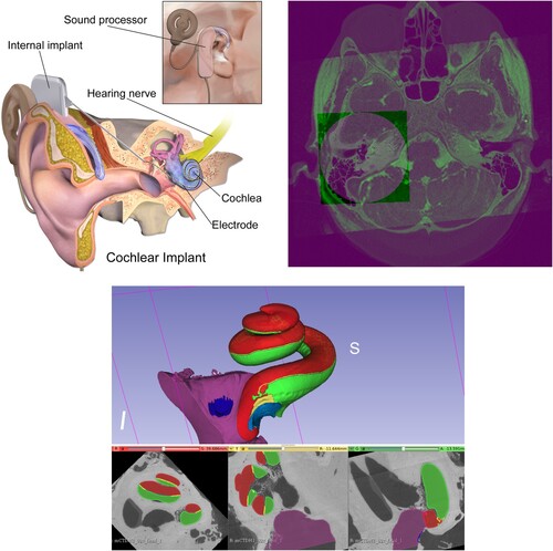
The Cochlear Duct Length (CDL) may have a significant impact on the selection of the cochlea implant (CI) type, see Figure 1 top left. An inappropriately-sized CI could result in unsuitable frequency-place mapping between the CI electrode array and the auditory nerve. An overly long electrode may only partially insert into the cochlea, resulting in extracochlear electrode contacts, whereas an electrode that is too short may result in inadequate cochlear coverage (Mistrak & Jolly 2016; Iyaniwura et al. 2018).

Figure 1 Top left: Cochlea and cochlear implant components. Top right: Fused cochlea image from CBCT, CT, and MR images. Bottom: Cochlear image segmentation of μCT showing the cochlea main scalae. Scala tympani in green and both scala vestibuli and scala media in red (top: 3D view: bottom from left to right: axial, sagittal, and coronal views).

To obtain relevant preoperative information from medical images of the cochlea before CI surgery, radiologists use a manual procedure which requires expertise and is time-consuming. Automating this manual procedure is a challenging problem due to the low-resolution of clinical cochlear images, their small size, and the complicated structure of the cochlea.

Another important application for automating cochlear image analysis is the use of surgical robots. These robots rely on real-time computer vision algorithms, e.g. object detection, segmentation, and analysis. A cochlear surgical robot (Weber et al. 2017) requires reliable real-time estimations of the length and volume of the cochlea to decide which CI is appropriate for a specific patient. This study proposes an automated fast cochlear length and volume estimation that has the potential to benefit both cochlear surgeons and robotic surgeries.

1.1. Cochlear image registration

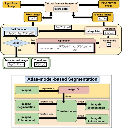
Image registration (Hajnal et al. 2001; Yoo 2012; Goshtasby 2004) is the main element in atlas-based segmentation methods (Rohlfing et al. 2005), and efficient image registration methods produce more accurate image segmentation. Figure 1 (top right) shows an example of registered and fused cochlear images from CBCT, CT, and MR of the same patient.

Image registration is the process of finding parameters μ of a transformation T that aligns one or more images to an image called the fixed image. Atlas-based segmentation is an inter-subject image registration as it aligns a model to images of different patients. Inter-subject image registration is more challenging than intra-subject image registration because of the difference in the shape and size of the objects in the input images. Mathematically, the transform can be written as a function of the image points P and the transform's parameters μ. A simple example is the 2D translation transform: (1) $T(p_i,\mu )=T((x_i,y_i),({\mu }_0,{\mu }_1))=(x_i+{\mu }_0,y_i+{\mu }_1).$(1) Image registration uses transformation parameters to transform an image, called a moving image $I_M(P)$, to another image, called a fixed image $I_F(P)$. Finding these parameters is challenging and the general registration problem is still unsolved. Every year, many scientific articles are published in the field of image registration which signifies the importance of this problem.

The transformation must either be a non-rigid transformation, e.g. affine or B-spline transforms, or a composed transformation that includes a non-rigid transformation. This is needed to address the difference between the size and shape of different patients' cochleas.

In B-spline (Unser 1999) transform, the deformation field is modelled using B-spline control points. This offers a desirable non-linear effect, allowing for the deformation of certain parts of images without impacting others. The disadvantage of this transform is that the number of parameters is very large which requires more time and resources for computation.

The multimodal Automatic Cochlear Image Registration (ACIR-v2 and ACIR-v3) were proposed by Al-Dhamari et al. (2017, 2022) as a practical cochlear intra-subject image registration method for multimodal images of the same patient. They align all three modalities, i.e. CT, MR, and CBCT to the same space. The main idea is to crop original input images to the cochlear part and register them. This produces a faster and more accurate transformation that registers the original images. ACIR-v2 uses the Adaptive Stochastic Gradient Descent (ASGD) optimiser (Klein et al. 2009) to minimise negative Mattes' Mutual Information $S_{\mathrm{MMI}}$ similarity metric (Mattes et al. 2001) of two images by updating three-dimensional (3D) rigid transformation parameters.

Gradient descent (GD) is an optimisation algorithm used to minimise a cost function. The algorithm works by adjusting the parameters incrementally, reducing the cost (or ‘error’) by calculating the negative gradient (the steepest descent) at the current position in the cost function. This way, it gradually moves towards the function's local or global minimum. The step size (or the learning rate) determines the size of the steps during this iterative process. Stochastic Gradient Descent (SGD) is a variant of gradient descent, designed to handle large datasets more efficiently. Instead of calculating the gradient using the whole dataset (which can be computationally expensive), SGD takes a random sample (one or a small batch) at each step. This introduces some noise into the process, which can help escape local minima, but also might make the descent path more erratic. ASGD is another modification of the basic SGD that adapts the step size for each parameter during the optimisation. It helps in faster convergence and can eliminate the need of manually tuning the step size.

This optimisation process is fast as it only involves small images as a result of the cropping. Only one manual step is required which is the localisation. However, it is only needed for cropping. The average time reported for aligning a pair of images, using a standard laptop, was $10.84\pm 3.12$ seconds.

1.2. Cochlear image segmentation

Efficient automatic segmentation algorithms may help to automate cochlear image analysis. Image segmentation (Gonzalez & Woods 2006) is defined as the process of extracting one object, which is similar to binary classification, or more objects, which is similar to multi-class classification, from an input image, see Figure 1 bottom.

Atlas-based image segmentation (Rohlfing et al. 2005) uses image registration concept to align an atlas or a predefined segmentation to an input image. The atlas is usually a well-defined histological image or a high-resolution micro-Computed Tomographic (μCT) image, as in Figure 1 bottom.

Model-based segmentation methods (Cootes et al. 1995; Edwards et al. 1998) on the other hand try to fit a statistical shape model to the input image. The model is generated using many segmentation images.

Artificial intelligent and deep learning methods are used in a number of recent articles. However, the models work only on either CT or MRI scans not both. Moreover, they do not segment the cochlea scalae.

In Vaidyanathan et al. (2021), the authors used 3D U-net (Ronneberger et al. 2015). They used 944 MRI scans for training and 177 MRI scans for testing from three different centres. Their model showed Dice score of 0.8768. The Dice score, or Dice coefficient, is a statistical tool used for comparing the similarity of two samples. It ranges between 0 (no overlap) and 1 (perfect match) (Sorensen 1948).

In Liu et al. (2022), the authors proposed a cochlear segmentation method based on a cross-site cross-modality unpaired image translation strategy and a rule-based offline augmentation. They adopted a self-configuring segmentation framework empowered by self-training. They used Contrast-enhanced (ce) T1 and High-resolution (hr) T2 MRI images from the crossMoDA challenge (Dorent et al. 2023). They used 210 ce T1 and 210 hr T2 for training. For validation, they used 64 hr T2. They showed mean Dice scores of $0.8433\pm 0.0293$.

In Han et al. (2017), the authors used nnU-Net model (Isensee et al. 2021) for cochlear segmentation. They used the same dataset from the crossMoDA challenge. They showed a dice score of 0.8394. Their source code is provided.

In Li et al. (2022), the authors proposed a semi-supervised GAN model called GSDNet. They used 30 cochlea CT slices. They showed that their model achieved 93.73 Dice score. However, the model only works on 2D CT cochlea images and it does not segment the cochlea scalae.

ACIR-v2 was used in Automatic Cochlea Analysis (ACA) method which combined atlas-based and model-based methods in Al-Dhamari et al. (2018) for cochlear segmentation and analysis. The method aligned an image with a predefined detailed segmentation and a predefined points model to an input image. After that, it used the resulting transformation to transform the predefined segmentation and the points model to the input image, see Figure 2. The points model was used to estimate the length of the scala tympani.

Figure 2 Top: Image registration basic components. Bottom: Atlas–model-based concept.

1.3. Cochlea image analysis

The literature shows major variations in the measurements of human CDL. The main methods were image processing and spiral coefficient equations.

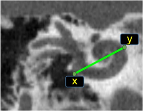
In Escude et al. (2006), an equation for the spiral coefficient was introduced that requires only one measurement called A-value. It was defined as the greatest distance from the round window to the opposite cochlear lateral wall, e.g. the length of the line connecting point x to point y in Figure 3. This equation was improved in Alexiades et al. (2015) and Koch et al. (2017a) using a linear equation.

Figure 3 Cochlea A-value method. The green points (x, y) are the A-value end points, the green line shows the A-value length.

In Iyaniwura et al. (2018), a method to measure A-value automatically was proposed. It was tested using conventional and μCT images of cadaveric cochlear specimens. The main disadvantage of the A-value based methods is their need for a very clear and sharp image. Therefore, it cannot be measured accurately in the case of MR images or images affected by noise.

To compute the scala tympani lateral wall (StLt) and organ of corti (StOc) lengths, these equations are needed: (2) $\mathrm{StLt}=A\ast 3.86+4.99,$(2) (3) $\mathrm{StOc}=A\ast 4.16-5.05,$(3) where A is the A-value length in mm.

In Weurfel et al. (2014), 3D reconstructions of cross-sectional imaging were used to measure the cochlear length of the CBCT of the temporal bones. The cochlear length was measured from the distal bony rim of the round window to the helicotrema using a 3D curve set up from the outer edge of the bony cochlea.

In Koch et al. (2017b), the CDL and the relation between the basal turn lengths and CDL were computed using 3D multi-planar reconstructed CT images.

In Rivas et al. (2017), comparisons were made between CDL computed from automatic A-value, 3D reconstruction, and CDL computed from manual A-value. They mentioned that automatic method results were reproducible and less time-consuming.

In Koch et al. (2017b), the authors reviewed the literature related to the CDL measurement and analysed results from different methods, e.g. direct measurement CDL from histology, reconstructing the shape of the cochlea, and determining CDL based on spiral coefficients. They concluded that the 3D reconstruction method is the most reliable method to measure CDL because it provides visualisation of the cochlea.

In Al-Dhamari et al. (2018), a combined atlas–model-based method was used to measure CDL based on a points model. The method used the actual length of the CI as ground truth to estimate the error resulting from the image artefact. A segmentation of the electrodes array was performed, then the length was computed. Thereafter, the estimated error was computed by comparing the computed electrodes array's length to its actual length.

The estimated error average of the CI length was 0.62 mm ± 0.27 mm. The average estimated scala tympani length and volume were computed from 71 cochlea images. The average estimated scala tympani length was $29.54\pm 0.27$ mm. The average of the estimated scala tympani volume was $41.56\pm 0.19$ mm${}^3$. This method uses a rigid transformation which does not address the difference in volume and shape of different patients.

In Heutink et al. (2020), the authors proposed deep learning methods for cochlea detection, segmentation, and measurement. They used 123 CT scans (40 for training, 8 for validation, and 75 for testing). The detection model is a classification model that outputs a probability map with values close to 1 in image locations where the cochlea is more likely to be present. The segmentation model is a U-net-like architecture composed of an encoder–decoder structure. The authors used a combination of convolutional neural networks and thinning algorithms in addition to the A-value equation proposed by Alexiades et al. (2015) to compute the basal diameter, and cochlear duct length from the segmentation result. The cochlear volume was measured directly from the segmentation result by counting the voxels. Automatic segmentation was validated against manual annotation and the mean Dice was 0.90±0.03. Automatic cochlear measurements resulted in errors of 8.4% (volume), 5.5% (CDL), 7.8% (basal diameter). The cochlea volume was between 0.10 and 0.28 mm${}^3$. The basal diameter was between 1.3 and 2.5 mm and CDL was between 27.7 and 40.1 mm.

The development of a more consistent, less time-consuming, and reproducible method for CDL is still needed.

2. Material and methods

2.1. Dataset

Ethics statement:

The use of all medical images in our experiments was approved by the Ethics Committee of the Rheinland-Pfalz state, Germany (Landesaerztekammer Rheinland-Pfalz, Koerperschaft des oeffentlichen Rechts) with request number 2021-15895-retrospektiv, and the research ethic committee (REC) Ain Shams University, Cairo, Egypt, with request number R136/2021. The datasets are not publicly available due to restrictions from the hospitals. Formal email requests and acceptance of the ethics committee are required to obtain copies of the datasets.

The term dataset in this study means a collection of 3D medical images. In this study, two datasets from different geographical locations were used. The patients' information was anonymised to protect their privacy. These datasets contained 3D cochlear images of different modalities, i.e. MR, CT, and CBCT. The total number of images was 219 multimodal 3D images of 67 patients of mixed gender and age from two datasets, G and E.

The G dataset represents a dataset from Germany and contains 168 images of 41 patients. It includes 75 MR, 18 CT, and 75 CBCT images. The E dataset represents a dataset from Egypt and contains 51 images of 26 patients. The number in the table is different as some images were used only in one of the experiments. It includes 28 CT and 23 CBCT images. Some details about the dataset are available in Table 1. To our knowledge, this is the first study of its kind that includes CT, CBCT, and MR images from two different populations.

Table 1 Datasets, images used in both experiments: 108

	Automatic experiments			Manual experiments
	G	E	Total	G	E	Total
Patients	41	26	67	34	26	60
Images	168	49	217	66	46	112
CBCT	75	23	98	57	18	75
CT	18	26	44	9	28	37
MR	75	0	38	0	0	0
Left	80	24	104	33	22	55
Right	88	25	113	33	24	57
Before surgery	125	25	104	34	25	59
After surgery	43	24	67	32	21	53

All the MRI images are T2 images that represent the patient's status before CI surgery. Each image has a size of $384\times 512\times 64$ voxels with $0.39\times 0.39\times 0.7$ mm spacing. All the images belonging to the G dataset were obtained using ‘Siemens Skyra 3 Tesla’ and ‘Siemens Avanto 1.5 Tesla’ scanners.

CBCT images from the G dataset were obtained using a ‘Morita 3D Accuitomo 170’ scanner. These images represent one side only, either the left ear or the right ear. Post-CI surgery CBCT images have a size of $485\times 485\times 121$ voxels with $0.12\times 0.12\times 0.5$ mm spacing. Pre-CI surgery CBCT images have a size of $483\times 48\times 161$ voxels with $0.12\times 0.12\times 0.3$ mm spacing.

These CBCT images were probably cropped by the radiologist as they do not have isotropic spacing. CT images from G dataset were obtained using a ‘Siemens Sensation Cardiac 64’ scanner. All CT images were taken before CI surgery as was the case with MR images.

Each CT image has a size of $512\times 512\times 58$ voxels with $0.12\times 0.12\times 1.0$ mm spacing. The CBCT images from E dataset were obtained using an ‘i-CAT Next Generation’ scanner with the following protocol: 120 kvp, 5 mAs, voxel 0.2, matrix = 0.2.2.2 mm. FOV 2.5 cm, with 7 seconds exposure time and 14.7 seconds scanning time. The CT images from E dataset are obtained using a ‘Siemens Somatom Definition flash SD dual source 64 row’ scanner with the following parameters: KV, 100–140 mA 100–800, with pitch factor 0.55–1.5, ratio using one X-ray source and a single collimation width of 0.6 mm.

2.2. Experiments

We've conducted a series of experiments, applying various methods to the image datasets to obtain diverse cochlea measurements. Two distinct studies were conducted in this context. A total of 217 experiments were carried out. In the first study, 112 images were examined separately to obtain manual measurements of the A-value. A set of 108 images from this batch was then utilised in the second study, in which both automatic and manual methods were applied concurrently. For a more in-depth view, please refer to Table 1. The reason for the omission of certain images from the second study was due to high noise levels in these images, making it difficult for even experts to determine an approximated ground truth.

The cochlear structure, i.e. cochlear scalae, is invisible in clinical images. Since the round window and the top of the cochlea can be located approximately in these images, landmarks can be a useful tool for validation and error estimation.

The accuracy of the method was evaluated using the Root Mean Squared Error (RMSE) of two 3D point landmarks located by two head and neck radiology experts.

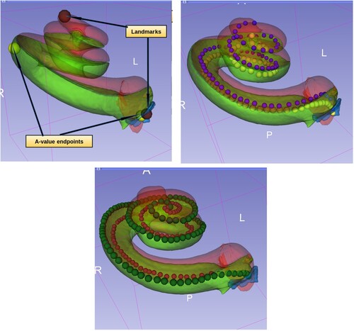
The landmarks represented the cochlear round window and the cochlear apex (helicotrema), see Figure 4 top. There should be a small human error here, see the study limitations section. The total number of landmarks used was 434. After aligning the model to the input image, the landmarks of the model were transformed by the same resulted transformation to the input image. Thereafter, RMSE in mm was measured between these transformed landmarks and the related input image landmarks. This gave a quantitative estimation of the error and provided an evaluation of the proposed method. The standard open-source software 3D Slicer was used for visualisation purposes (Kikinis et al. 2014).

Figure 4 Top left: Cochlea landmarks in brown colour and A-value endpoints in yellow colour. Top right: The point models of scala tympani (in yellow) and scala vestibuli (in blue) central lengths. Bottom: The point models of scala tympani, the outer points in dark green colour for measuring the lateral wall length and the inner points in dark red for measuring the organ of corti length.

2.3. Evaluation

The time required to obtain the segmentation and all measurements (including the cropping process) has been recorded. The total time includes loading the image file, cropping, registration, segmentation, and analysis. The experiments are done multiple times automatically using a python script. The locating process was done manually for all images before running the script. The locating process is not included in the total time.

Since the result time recorded might differ according to the hardware used, all the experiments of ACA-v2 were done using the same hardware. The hardware used was a computer equipped with an AMD Ryzen 3900 CPU, a 32 GB memory and Nvidia RTX2080Ti graphics card. We used the same parameters and the original implementations of ASGD and the stochastic Limited-memory Broyden–Fletcher–Goldfarb–Shanno (s-LBFGS) (Qiao et al. 2015) which are provided in the elastix 5.0.0 toolbox (Klein et al. 2010). The LBFGS algorithm is a quasi-Newton method that approximates the Hessian matrix to guide the search direction. The ‘limited-memory’ aspect denotes its ability to utilise a low amount of computer memory, making it suitable for problems with a large number of variables.

The experiment was repeated three times and the average values were used. To obtain detailed information, the images were divided into different groups based on their types: CBCT, MR, CT, and images with a cochlear implant (CI). This allowed for the collection of more detailed data on the proposed method's performance on each specific modality. The total results were also presented as well to give a global evaluation.

The same measurements should be reported from the same patient's images, e.g. the cochlear length from an MR image and from a CT image of the same patient should be the same. We defined the difference as In-Patient-Error (IPE) which is the error that results from image artefacts produced by different scanners. IPE was computed for all measurements of three methods: ACA-v2, automatic, and manual A-value.

The results were validated using standard statistical bootstrapping with 1000 iterations, paired and independent t-test (Diez et al. 2019). This ensured that the result means were accurate estimates of the population means.

2.4. The proposed method (ACA-v2)

The proposed Automatic Cochlea Analysis (ACA-v2) method used an atlas–model-based segmentation to align predefined segmentation and point models to an input image. The predefined segmentation served as an atlas. It was manually segmented using a high-resolution μCT image obtained from a public and standard μCT cochlear dataset (Gerber et al. 2017; Al-Dhamari et al. 2018).

Th2e original μCT was resampled from $0.008\times 0.008\times 0.008$ mm spacing to $0.032\times 0.032\times 0.008$ mm spacing. The image size was reduced to 806 MB from 13.4 GB. ITK (Yoo et al. 2002) and 3D Slicer software were used for resampling.

Next, a cropping process was performed to crop the cochlear part from the input image. This allowed for a smaller image size of 103.2 MB with $243\times 202\times 1191$ voxel elements (voxel) instead of $437\times 412\times 2349$ voxels. After that, the two main cochlear scalae, i.e. scala vestibuli and scala tympani, were segmented manually, see Figure 1 bottom. The model and its segmentation were cloned and transformed to represent left and right cochlear sides. The transformed models were automatically aligned to one of the clinical CBCT images using ACIR-v3 (Al-Dhamari et al. 2022). The atlases were aligned using the same method. A user-friendly interface for the atlas-based segmentation method was developed as a Slicer extension.¹ A video demonstrating how to use the tool is available at https://www.youtube.com/watch?v=jHD3GKepDLs.

Skeletonisation methods (Gonzalez & Woods 2006) help to obtain thinner objects from source objects and help create lines and curves which can be used for measuring lengths. Unfortunately, skeletonisation methods did not work in the cochlea case due to the non-regular shape of the cochlear scalae (Al-Dhamari et al. 2018). The authors of Al-Dhamari et al. (2018) proposed creating a points set model for cochlear measurement purposes. It contained 55 points representing the centre of the scala tympani. Using the transformed points set, the length of the scala tympani could be calculated by computing the distance between every two consecutive points using (4) $\mathrm{Length}=\sum _{i=1}^{n-1}\sqrt{(x_{i+1}-x_i{)}^2+(y_{i+1}-y_i{)}^2+(z_{i+1}-z_i{)}^2}$(4) where n is the number of the points, and x, y and z are the coordinates of the 3D points. This approach was faster than skeletonisation as it includes only one simple matrix multiplication. Moreover, the points could be corrected or modified manually later to produce different useful measurements (e.g. measuring the inner or outer length of a scala).

This study introduces five main contributions:

(1)	We improved ACA (Al-Dhamari et al. 2018) by adding a second stage non-rigid registration that uses B-spline transformation. This addressed the difference between the input images of different patients and the model. Using non-rigid registration gave more accurate deformation and more realistic measurements. Algorithm 1 lists the steps of the new proposed method, Automatic Cochlea Analysis (ACA-v2).
(2)	ACIR-v2 was replaced by ACIR-v3 method (Al-Dhamari et al. 2022) which is a more recent method that uses a stochastic quasi-Newton optimiser.
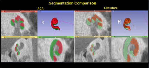
(3)	A higher resolution cochlea atlas was used which produced more accurate results. Figure 5 shows what ACA-v2 result looks like compared to ACA (Al-Dhamari et al. 2018).
(4)	We added four more point sets to automate the process of measuring different lengths. For each model, we increased the number of points to increase the accuracy of the curve measurements. ACA-v2 included these point models, see Figure 4: Scala vestibuli points model (SvPt): Points that go through the centre. Scala tympani points model (StPt): Points that go through the centre. Scala tympani lateral wall points model (StLt): Points that go through the outer wall. Scala tympani organ of corti points model (StOC): Points that go through the inner wall (the organ of corti). A-value endpoints model: End points of the A-value method. This helps to automate the process of measuring the A-value and calculating the scala tympani lateral wall and organ of corti lengths using the A-value method automatically.Using these point models, one can get all standard measurements from different methods, e.g. A-value which helps doctors decide the best implant type for a specific patient. ACA-v2 has the advantage that it works on any type of image even when high noise is present. Using these point models, one can calculate all required standard measurements from different methods.
(5)	Multiple datasets were used from different geographical locations which gave more informative results and statistics.

Figure 5 Cochlear segmentation using the new proposed high-resolution atlas in comparison to the low-resolution atlas proposed in ACA (Al-Dhamari et al. 2018).

Algorithm 1. ACA-v2

Input: Multimodal 3D clinical cochlea image I(P)

Output: Cochlear segmentation and different measurements

1: Locate the cochlea locations in input images

2: Crop the cochlea part into a smaller image: $\tilde{I}(P)$= Crop($I(P)$)

3: Apply ACIR-v3 on the cropped input image and the predefined image:

4:    $I_{\mathrm{res},T}=(\tilde{I}(P),I_M(P))$

5: Register the resulted image with the model image using B-spline transform:

6:   T= register $({\tilde{I}}_{\mathrm{res}0},I_M(P))$

7: Transform the segmentation and the point models:

8:   $I_{\mathrm{seg}}(P)=I_{M_{\mathrm{seg}}}(T(P),\mu )$, $I_{\mathrm{points}}(P)=I_{M_{\mathrm{points}}}(T(P),\mu )$

9: Output the segmentation and cochlea the measurements

3. Results

The total RMSE average was $0.61\pm 0.22$ mm. For the CBCT with implant group, the average RMSE was $0.54\pm 0.17$ mm. The CBCT without implant group had an average RMSE of $0.60\pm 0.18$ mm, while the CT group showed an average RMSE of $0.64\pm 0.17$ mm. As for the MR group, the average RMSE was $0.60\pm 0.25$ mm, see Figure 7 top. Sample results are shown in Figure 6.

Figure 6 Sample of the results from different image types with RMSE values. In each group, the image on the left has the lowest RMSE value and the image on the right has the highest RMSE value. Each result has the 3D model at the top and the three standard views at the bottom, i.e. axial, sagittal, and coronal.

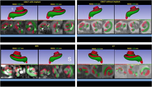
Figure 7 Sample from the results: RMSE and time charts of different image groups. CBCT after and before surgery, CT, and MR.

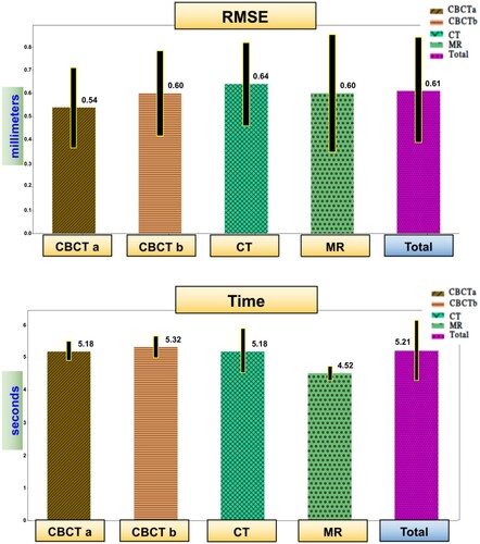
The average total time required for analysing an image was $5.21\pm 0.93$ seconds. The CBCT with an implant group resulted in an average time of $5.18\pm 0.27$ seconds. CBCT without an implant group had an average time of $5.32\pm 0.3$ seconds. The CT group presented an average time of $5.18\pm$ seconds, and for the MR group, it was $4.52\pm$ seconds, see Figure 7 bottom.

IPE was computed for all measurements of three methods: ACA-v2, automatic, and manual A-value. In Figure 8, a comparison between manual and automatic A-value methods is shown.

Figure 8 Sample from the results: In-Patient-Error in mm. The comparison between automatic A-value method and manual A-value method (Lt and Oc are short for lateral wall and organ of corti).

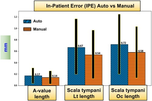
The measurements included the average of the estimated scala vestibule length and volume, the average of the estimated scala tympani volume and different lengths, and the A-value. Scala vestibuli was actually the combined scala media and scala vestibuli. The length measurements included a length that passed through the centre of the scala (central length). Additional lengths were recorded for the scala tympani as it is of more interest due to the fact that it is the site of the cochlea implant. These lengths passed through the scala lateral wall and the organ of Corti, see Figure 4. They were computed using three methods: ACA-v2, an automatic A-value, and a manual A-value. In Tables 2 and 3, the cochlear measurements and their IPE values are listed from all the tested cochlea images (STD is short for standard deviation).

Table 2 ACA-v2 measurements with IPE

	Scala vestibuli volume (mm${}^3$)	Scala tympani volume (mm${}^3$)	Scala vestibuli centre length (mm)	Scala tympani centre length (mm)
Mean	41.69	48.57	35.95	30.06
Std	2.0	2.24	0.53	0.45
Min	34.98	38.98	35.21	29.53
Max	49.3	57.67	38.79	32.21
IPE mean	1.79	1.91	0.61	0.52
IPE STD	1.26	1.3	0.47	0.4

Table 3 Scala tympani length measurements with their In-Patient-Error (IPE)

Length (mm)	A-value		Scala tympani lateral wall			Scala tympani organ-of-corti
Method	ACA-v2	Manual	ACA-v2	A-value auto.	A-value manual	ACA-v2	A-value auto.	A-value manual
Mean	8.96	9.02	43.88	39.58	39.82	31.77	32.23	32.49
STD	0.17	0.45	0.74	0.67	1.72	0.54	0.72	1.86
Min	8.75	8.21	42.93	38.75	36.69	31.11	31.34	29.12
Max	9.57	10.06	47.19	41.92	45.91	34.08	34.75	39.05
IPE mean	0.17	0.14	0.73	0.67	0.54	0.53	0.72	0.58
IPE STD	0.13	0.11	0.57	0.48	0.42	0.41	0.52	0.45

The overall volume of the cochlea ranged from 73.96 to 106.97 mm${}^3$ and the scala tympani length ranged from 42.93 to 47.19 mm (lateral wall) and from 31.11 to 34.08 mm (organ of corti).

The statistical tests showed that there was no statistically significant difference between the results from the automatic A-value method and the manual A-value method (P-value = 0.42). Similarly, there was no significant difference between the lengths measurements of the left and right ear sides (P-value > 0.16).

Upon comparison of the results derived from the two datasets, it became evident that the difference was not significant when utilising either manual or automatic A-value methods (P-value > 0.20). However, in the case of employing the ACA-v2 method, there was a significant deviation observed, compared to the results from the manual or automatic A-value methods (P-value < 0.001).

4. Discussion

In this study, we proposed a practical solution for solving the clinical multimodal 3D cochlear image segmentation and analysis problem. This problem has important applications related to cochlear implant surgery and cochlear research. The proposed method was tested and worked successfully on CBCT, CT, and MR images. The method has been validated using different datasets.

In Iyaniwura et al. (2018), the authors used the same idea of cropping and points model which was originally proposed in ACA (Al-Dhamari et al. 2017, 2018). They replaced the points model of the scala tympani with a points model of the A-value end-points. They used clinical and micro-CT images of 20 cadaveric cochleae specimens. A-value fiducials were placed onto a selected micro-CT to be used as an atlas. Multi-registration (rigid affine and non-rigid B-spline) was applied between the atlas and the 19 remaining clinical CT images. However, their work was tested on a small number of images. Moreover, the clinical CT images were obtained using the same cadaveric cochleae specimens. They did not report the registration parameters nor the time.

Our results showed that automatic A-value, which is a part of ACA-v2 that we proposed, produced results that match those produced manually by experts. The IPE between them was only 0.03 mm. All average lengths were close to each other, but STD was slightly greater in the case of the manual results. Since these manual experiments were done only by two experts, the results may be affected by some human error during location of the A-value points.

The measurement results of the G and E datasets were concordant. The averages from the automatic and manual method experiments were close in both datasets. This is probably due to the small number of patients (67 patients in total, 41 from the G dataset and 26 from the E dataset). However, there was a large difference in the tympani lateral wall length from ACA-v2 compared to the A-value (about 4 mm). The lateral wall length from A-value probably does not cover the complete scala tympani which is not the case in ACA-v2 length.

ACA-v2 provided more accurate measurements that captured small differences between different people. The length from ACA-v2 method can be visualised and had well-defined end-points. The ACA-v2 method worked on different modalities and different images despite varying noise levels and resolutions. On the other hand, the A-value method worked neither on MR nor on noisy images of other modalities. Hence, ACA-v2 method may provide more reliable and accurate measurements than the A-value method.

4.1. Study limitations

First, the proposed method required a manual step to locate the cochlea. This manual step can be solved efficiently in the future, e.g. using Haar feature-based cascade classifiers (Viola & Jones 2004) or Yolo (Redmon et al. 2016). However, the image registration and segmentation was done automatically without human interference.

Second, the ground truth landmarks were created by only two human experts. This the first time that such landmarks for clinical images have been created. There should be a small human error, e.g. the round window typically spans multiple voxels and not a single point. There should be variability when picking the similar point each time. To reduce human error, more experts should be involved.

Finally, the proposed method only used one model. To account for cochlear abnormalities and different shapes, more models should be used to create a statistical shape model. However, the method provided a friendly user interface for visualisation and manual correction of the measurements when needed.

5. Conclusion

ACA-v2 provided more accurate measurements that captured small differences between different people. The length from ACA-v2 method can be visualised and had well-defined end-points. The ACA-v2 method worked on different modalities and different images despite varying noise levels and resolutions. On the other hand, the A-value method worked neither on MR nor on noisy images of other modalities. Hence, ACA-v2 method may provide more reliable and accurate measurements than the A-value method.

We proposed a novel method, ACA-v2, that helps to visualise required cochlea's lengths and show curve end-points. This method also works on different modalities whereas the A-value method may not provide accurate results when use with MR or noisy images of other modalities.

The experiments were repeated three times to ensure the reliability of the results. Standard statistical tests were used to validate the results. The proposed method has been made available as a public open-source extension for 3D Slicer software so that other researchers can reproduce these results.

Future works should include further improvements in speed and accuracy of the method. Future research should also include the utilisation of a better histological model to provide segmentation of the three cochlear scalae.

There is also potential to explore what deep learning and statistical shape models could contribute to this method. To improve the ground truth, more datasets from different geographical locations and more experts should be involved to provide more landmarks and manual segmentation for evaluation.

Disclosure statement

No potential conflict of interest was reported by the author(s).

Additional information

Funding

The author(s) reported there is no funding associated with the work featured in this article.

Notes on contributors

Ibraheem Al-Dhamari

Dr. Ibraheem Al-Dhamari is an expert in computer vision and medical informatics. Currently, he holds a postdoctoral position at the Medical Informatics Department of BIH@Charité in Berlin, Germany. He earned his PhD in computer vision from the University of Koblenz, Germany. Dr. Al-Dhamari's research spans across areas such as medical image analysis, informatics, computer vision, image processing, machine learning, deep learning, biomechanical simulation, and cellular automata.

Rania Helal

Dr. Rania Helal, MD, is a lecturer at the Radiodiagnosis department, Faculty of Medicine, Ain Shams University, Egypt.

Tougan Abdelaziz

Prof. Tougan Abdelaziz is a professor at the Radiodiagnosis Department, Faculty of Medicine, Ain Shams University, Egypt. Oberstarzt Priv.-Doz.

Stephan Waldeck

Dr. Stephan Waldeck is the head of the Radiology/Neuroradiology department at the Koblenz military hospital. His research interest includes environmental impact assessments, PET/CT and PET-MRI imaging, interventional radiology, radiation therapy, ultrasound imaging, computed tomography, and magnetic resonance imaging.

Dietrich Paulus

Prof. Dietrich Paulus is the head of the Active Vision (AGAS) research group at the University of Koblenz. His research interest includes autonomous robots, medical image processing, machine learning, and computer vision.

Notes

1 https://github.com/MedicalImageAnalysisTutorials/SlicerCochlea.

References

- Al-Dhamari, I., Bauer, S., Paulus, D., Helal, R., Lisseck, F., Jacob, R. 2018. Automatic cochlear length and volume size estimation. In Or 2.0 context-aware operating theaters, computer assisted robotic endoscopy, clinical image-based procedures, and skin image analysis. Cham: Springer International Publishing, p. 54–61.
- Al-Dhamari, I., Bauer, S., Paulus, D., Lesseck, F., Jacob, R., Gessler, A. 2017. ACIR: automatic cochlea image registration. Medical Imaging 2017: Image Processing, 10133(10): 1–5.
- Al-Dhamari, I., Helal, R., Morozova, O., Abdelaziz, T., Jacob, R., Paulus, D., et al. 2022, 03. Automatic intra-subject registration and fusion of multimodal cochlea 3D clinical images. PLoS ONE, 17(3): 1–18. doi:10.1371/journal.pone.0264449
- Alexiades, G., Dhanasingh, A., Jolly, C. 2015. Method to estimate the complete and two-turn cochlear duct length. Otology and Neurotology, 36(5): 904–907.
- Cootes, F., Taylor, C., Cooper, D., Graham, J. 1995. Active shape models - their training and application. Computer Vision and Image Understanding, 61: 38–59.
- Diez, D., Cetinkaya-Rundel, M., Barr, C. 2019. Openintro statistics (4th ed.). Electronic Copy.
- Dorent, R., Kujawa, A., Ivory, M., Bakas, S., Rieke, N., Joutard, S., et al. 2023. CrossMoDA 2021 challenge: benchmark of cross-modality domain adaptation techniques for vestibular Schwannoma and cochlea segmentation. Medical Image Analysis, 83: 102628. doi:10.1016/j.media.2022.102628.
- Edwards, G.J., Taylor, C.J., Cootes, T.F. 1998. Interpreting face images using active appearance models. Proceedings Third IEEE International Conference on Automatic Face and Gesture Recognition, 1: 300.
- Escude, B., James, C., Deguine, O., Cochard, N., Eter, E., Fraysse, B. 2006. The size of the cochlea and predictions of insertion depth angles for cochlear implant electrodes. Audiology and Neurotology, 1: 27–33.
- Gerber, N., Reyes, M., Barazzetti, L., Kjer, H.M., Vera, S., Stauber, M., et al. 2017. A multiscale imaging and modelling dataset of the human inner ear. Scientific Data, 4(170132): 1–12.
- Gonzalez, R.C., Woods, R.E. 2006. Digital image processing (3rded.). Prentice-Hall, Inc.
- Goshtasby, A.A. 2004. Image registration: principles, tools and methods. London: Springer-Verlag. doi:10.1007/978-1-4471-2458-0
- Hajnal, J., Hill, D., Hawkes, D. 2001. Medical image registration. CRC Press.
- Han, L., Huang, Y., Tan, T., Mann, R. 2017. Unsupervised cross-modality domain adaptation for vestibular Schwannoma segmentation and Koos grade prediction based on semi-supervised contrastive learning. arXiv 1–10. doi:10.48550/arXiv.2210.04255
- Heutink, F., Koch, V., Verbist, B., van der Woude, W.J., Mylanus, E., Huinck, W., et al. 2020. Multi-scale deep learning framework for cochlea localization, segmentation and analysis on clinical ultra-high-resolution CT images. Computer Methods and Programs in Biomedicine, 191: 105387. doi:10.1016/j.cmpb.2020.105387
- Isensee, F., Jaeger, P.F., Kohl, S.A.A., Petersen, J., Maier-Hein, K.H. 2021, Feb 01. nnU-Net: a self-configuring method for deep learning-based biomedical image segmentation. Nature Methods, 18(2): 203–211. doi:10.1038/s41592-020-01008-z
- Iyaniwura, J.E., Elfarnawany, M., Ladak, H.M., Agrawal, S.K. 2018, Jan 22. An automated A-value measurement tool for accurate cochlear duct length estimation. Journal of Otolaryngology – Head & Neck Surgery, 47(1): 5.
- Kikinis, R., Pieper, S.D., Vosburgh, K.G. 2014. 3D Slicer: a platform for subject-specific image analysis, visualization, and clinical support. Intraoperative Imaging Image-Guided Therapy, 3(19): 277–289.
- Klein, S., Pluim, J., Staring, M., Viergever, M. 2009. Adaptive stochastic gradient descent optimisation for image registration. International Journal of Computer Vision, 81(3): 227–239.
- Klein, S., Staring, M., Murphy, K., Viergever, M.A., Pluim, J.P. 2010. elastix: a toolbox for intensity-based medical image registration. IEEE Transactions on Medical Imaging, 29(1): 196–205.
- Koch, R.W., Elfarnawany, M., Zhu, N., Ladak, H.M., Agrawal, S.K. 2017a. Evaluation of cochlear duct length computations using synchrotron radiation phase-contrast imaging. Otology and Neurotology, 38(6): e92–e99.
- Koch, R.W., Ladak, H.M., Elfarnawany, M., Agrawal, S.K. 2017b. Measuring cochlear duct length, a historical analysis of methods and results. Otolaryngology–Head and Neck Surgery, 46: 19.
- Li, Z., Tao, S., Zhang, R., Wang, H. 2022. GSDNet: an anti-interference cochlea segmentation model based on GAN. In: 2022 IEEE 46th annual computers, software, and applications conference (COMPSAC). p. 664–669. doi:10.1109/COMPSAC54236.2022.00114
- Liu, H., Fan, Y., Oguz, I., Dawant, B.M. 2022. Enhancing data diversity for self-training based unsupervised cross-modality vestibular Schwannoma and cochlea segmentation. arXiv 1–10. doi:10.48550/ARXIV.2209.11879
- Mattes, D., Haynor, D., Vesselle, H., Lewellen, T., Eubank, W. 2001. Non-rigid multimodality image registration. Medical Imaging 2001: Image Processing, 1: 1609–1620.
- Mistrak, P., Jolly, C. 2016. Optimal electrode length to match patient specific cochlear anatomy. European Annals of Otorhinolaryngology, Head and Neck Diseases, 133: 68–71.
- Qiao, Y., Sun, Z., Lelieveldt, B.P.F., Staring, M. 2015. A stochastic quasi-Newton method for non-rigid image registration. In N. Navab, J. Hornegger, W.M. Wells, A. Frangi, (eds.) Medical image computing and computer-assisted intervention – MICCAI 2015. Cham: Springer International Publishing, p. 297–304.
- Redmon, J., Divvala, S., Girshick, R., Farhadi, A. 2016, jun. You only look once: unified, real-time object detection. In: 2016 IEEE conference on computer vision and pattern recognition (CVPR). Los Alamitos, CA, USA: IEEE Computer Society, p. 779–788. doi:10.1109/CVPR.2016.91
- Rivas, A., Cakir, A., Hunter, J.B., Labadie, R.F., Zuniga, M.G., Wanna, G.B., et al. 2017. Automatic cochlear duct length estimation for selection of cochlear implant electrode arrays. Otology and Neurotology, 38(3): 339–346.
- Rohlfing, T., Brandt, R., Menzel, R., Russakoff, D.B., Maurer, J., Calvin, R. 2005. Quo vadis, atlas-based segmentation? the handbook of medical image analysis – volume III: registration models.
- Ronneberger, O., Fischer, P., Brox, T. 2015. U-Net: convolutional networks for biomedical image segmentation. In N. Navab, J. Hornegger, W.M. Wells, A.F. Frangi, (eds.) Medical image computing and computer-assisted intervention – MICCAI 2015. Cham: Springer International Publishing, p. 234–241.
- Sorensen, T. 1948. A method of establishing groups of equal amplitude in plant sociology based on similarity of species and its application to analyses of the vegetation on Danish commons. Kongelige Danske Videnskabernes Selskab, 4(1): 1–34.
- Unser, M. 1999. Splines: a perfect fit for signal and image processing. IEEE Signal Processing Magazine, 16(6): 22–38.
- Vaidyanathan, A., van der Lubbe, M.F., Leijenaar, R.T., van Hoof, M., Zerka, F., Miraglio, B., et al. 2021. Deep learning for the fully automated segmentation of the inner ear on MRI. Scientific Reports, 11(1): 2885. doi:10.1038/s41598-021-82289-y
- Viola, P., Jones, M. 2004, May 01. Robust real-time face detection. International Journal of Computer Vision, 57(2): 137–154. doi:10.1023/B:VISI.0000013087.49260.fb
- Weber, S., Gavaghan, K., Wimmer, W., Williamson, T., Gerber, N., Anso, J., et al. 2017. Instrument flight to the inner ear. Science Robotics, 2(4): 1–30.
- Weurfel, W., Lanfermann, H., Lenarz, T., Majdani, O. 2014. Cochlear length determination using cone beam computed tomography in a clinical setting. Hearing Research, 316: 65–72.
- Yoo, T.S. 2012. Insight into images: principles and practice for segmentation, registration, and image analysis. AK Peters Ltd.
- Yoo, T., Ackerman, M.J., Schroeder, W., Chalana, V., Aylward, S., Metaxas, D., et al. 2002. Engineering and algorithm design for an image processing API: a technical report on ITK - the insight toolkit. In: Proc. of medicine meets virtual reality. Amsterdam: IOS Press, p. 586–592.