Linear viscoelastic characterisation of bituminous mixtures using random stress excitations

Abstract

The three-dimensional linear viscoelastic characterisation of bituminous mixtures can be performed with the concurrent measurement of the complex Young's modulus and the complex Poisson's ratio. This normally requires the application of sinusoidal excitations leading to small strain amplitudes. Since in the linear domain the effects of sinusoidal excitations are independent of each other, the material behaviour can also be obtained using a broad-band multi-frequency excitation. In this study, the complex Young's modulus and Poisson's ratio of a bituminous mixture was obtained by applying a random wave axial stress to cylindrical specimens and measuring their strain response in the axial and transverse direction. The frequency response functions representing the Young's modulus and Poisson's ratio were calculated using a conventional spectral analysis approach. Sinusoidal tests at different strain levels were also carried out as a reference. Applying random waves at 10, 20 and 30°C provided results with a high signal-to-noise ratio at frequencies between 0.1 Hz and 40 Hz for the Young's modulus and between 1 and 90 Hz for Poisson's ratio. For both functions the results validate the time-temperature superposition principle. The direct comparison with the results of sinusoidal testing confirms the accuracy of the frequency response functions measured with the random wave approach and shows their potential for estimating the viscoelastic response of bituminous mixtures at infinitesimal strain level.

Keywords:

• linear viscoelasticity
• 2S2P1D model
• random excitation
• spectral analysis
• frequency response function

Introduction

The mechanical characterisation of bituminous mixtures at small strain levels aims at collecting fundamental information on their stiffness and dissipation properties for pavement design and analysis. The linear viscoelastic (LVE) theory and the time-temperature superposition principle (TTSP) provide the theoretical basis for this characterisation, and the complex Young's modulus $E^{\ast }$ is unanimously recognised as the most important and useful material property (Huang & Di Benedetto, 2015; Kim, 2008). However, since even in the isotropic case a second material property is necessary to solve 3-dimensional LVE problems, extensive research has been carried out to obtain the concurrent measurement of the complex Young's modulus and the complex Poisson's ratio ${\nu }^{\ast }$ (Di Benedetto, Delaporte, & Sauzéat, 2007; Graziani et al., 2018).

Available testing configurations for measuring $E^{\ast }$ and ${\nu }^{\ast }$ are categorised either as homogeneous, when they allow to measure axial stress and strain directly, or non-homogeneous when axial stress and strain need to be calculated indirectly, considering the specimen geometry as, for example, in bending or indirect tensile configurations (Di Benedetto, Partl, Francken, & Saint André, 2001). By definition, $E^{\ast }$ and ${\nu }^{\ast }$ are the ratio of sinusoidal functions, therefore sinusoidal loading histories are the first choice for experimental measurement (Graziani et al., 2017; Pham et al., 2015). Moreover, according to the LVE theory, $E^{\ast }$ and ${\nu }^{\ast }$ are also time and stress/strain independent parameters. Thus, measurements should be performed when the transient effects due to initial rest conditions are almost expired and the applied mechanical excitation should minimise the non-LVE effects on the response, like thixotropy, nonlinearity and of course damage (Di Benedetto, Nguyen, & Sauzéat, 2011). It has been shown that these latter effects become small, hopefully negligible, when the strain amplitude is also small. The small-strain domain for bituminous mixture may extend up to 100 μm/m, depending on the mixture properties and on the temperature (Airey, Rahimzadeh, & Collop, 2003), but significant changes of $E^{\ast }$ and ${\nu }^{\ast }$ have been observed well below 50 μm/m (Graziani, Bocci, & Canestrari, 2014b; Graziani, Cardone, & Virgili, 2016; Mangiafico, Babadopulos, Sauzéat, & Di Benedetto, 2018; Underwood & Kim, 2012; Uzan & Levenberg, 2007).

Besides sinusoidal testing, alternative methods based on wave propagation are used for characterising the behaviour of bituminous mixtures at small strains. These methods, which involve the high-frequency propagation of mechanical energy within the specimen, are also called dynamic or seismic methods. Larcher, Takarli, Angellier, Petit, and Sebbah (2015) provides a review of these methods focused on the measurement of the Young's modulus. Recently, dynamic methods have been used by several researchers to obtain the concurrent measurements of $E^{\ast }$ and ${\nu }^{\ast }$ (Carret, Di Benedetto, & Sauzeat, 2018; Carret, Pedraza, Di Benedetto, & Sauzeat, 2018; Gudmarsson, Ryden, & Birgisson, 2014; Gudmarsson, Ryden, Di Benedetto, & Sauzéat, 2015; Gudmarsson, Ryden, Di Benedetto, et al., 2014; Mounier, Di Benedetto, & Sauzéat, 2012). For the Young's modulus, results are generally in good agreement with those obtained by conventional sinusoidal test, as long as the strain level of the test is considered.

This study presents a methodology for measuring the complex Young's modulus and the Poisson's ratio of bituminous mixtures in the LVE domain using random stress excitations. The approach was originally developed by Virgili, Canestrari, and Graziani (2013) and is based on system identification algorithms. Random axial stress excitations are used to elicit the strain response of cylindrical specimens in the axial and transverse direction. With the assumption of linearity and isotropy, the frequency response function (FRF) representing the complex Young's modulus and Poisson's ratio is calculated and compared with those obtained by means of conventional sinusoidal tests carried out at various strain levels.

The system identification approach

Within the systems theory, system identification is a methodology that allows to infer the mathematical model of a physical system starting from the measurement of its input (excitation) and output (response) signals (Ljung, 1987). System identification focuses on systems for which the current value of the response depends not only on the current value of the excitation, but also on its earlier values (Oppenheim, Willsky, & Nawab, 1983). These systems are normally called dynamical systems. Linear time-invariant (LTI) systems are the most important class of dynamical systems. In the Fourier transform (FT) domain, they are represented by the input-output relation: (1) $Y\left(\text{j}\omega \right)=H\left(\text{j}\omega \right)X\left(\text{j}\omega \right)$(1) where $X\left(\text{j}\omega \right)$ and $Y\left(\text{j}\omega \right)$ are the FT of the input and output signals, respectively, and $H\left(\text{j}\omega \right)$ is the FT of the impulse response function, also called the frequency response function (FRF) of the system. In mechanics, Equation (1) represents the Hooke's law in the FT domain and is used to represent the LVE behaviour (Tschoegl, 1989). This establishes the formal analogy between LTI systems and LVE materials.

Among the nonparametric identification techniques that can be used to estimate the FRF, the simplest is the classical frequency-response analysis (Ljung, 1987). In this case, the system is excited using sinusoidal excitations of fixed frequency ($x_0\cdot \exp \text{(j}\omega t)$) and its steady-state response is measured, at each frequency, in terms of amplitude and phase shift ($y_0\cdot \exp \text{[j(}\omega t+\delta \left)\right]$). Based on Equation (1) the FRF is estimated directly as: (2) $H\left(\text{j}\omega \right)=\frac{y_0}{x_0}\exp \left(\text{j}\delta \right)$(2)

For characterising the LVE behaviour, strain/stress histories are used as excitation while stress/strain is the measured response. Sinusoidal testing is repeated at a certain number of frequencies (frequency sweep), within a range that is normally dictated by the material properties and by the testing equipment. Since sinusoidal signals pass through LTI systems independently of each other, they do not need to be excited separately at each frequency. In fact, the FRF may be estimated exciting the material with a generic random signal composed of a broad band of frequencies. In this case, the FRF can be obtained directly as the ratio of the FT of response and excitation (Equation 1). In practice, this approach leads to a very rough estimate of the FRF because of the presence of experimental noise (disturbances in the measurements of stress and strain). From Equation (1) we obtain a different formulation for the FRF: (3) $H\left(\text{j}\omega \right)=\frac{Y\left(\text{j}\omega \right)\overline{X\left(\text{j}\omega \right)}}{X\left(\text{j}\omega \right)\overline{X\left(\text{j}\omega \right)}}=\frac{{\mathrm{\Phi }}_{xy}\left(\text{j}\omega \right)}{{\mathrm{\Phi }}_x\left(\text{j}\omega \right)}$(3) where $\overline{X\left(\text{j}\omega \right)}$ is the complex conjugate of $X\left(\text{j}\omega \right)$, ${\mathrm{\Phi }}_x\left(\text{j}\omega \right)$ is the spectrum of the input signal and ${\mathrm{\Phi }}_{xy}\left(\text{j}\omega \right)$ is the cross-spectrum of the input and output signals. In this study Equation (3) is solved numerically using the MATLAB System Identification toolbox which adopts statistical methods for spectral estimation (Ljung, 1987, 2018).

Materials and methods

Materials

One AC mixture for wearing course is considered in this experimental study. It was produced in a central asphalt plant with a 70/100 pen bitumen, dosed at 5.3% (by aggregate mass). The limestone aggregate is characterised by a dense-graded curve, with a nominal maximum aggregate size of 11 mm. Cylindrical samples with diameter of 150 mm were produced using a gyratory compactor. They were subsequently cored to a diameter of 94 mm and cut to a length of 120 mm for performing the mechanical tests. The air voids content of the tested specimens was 9.6% and 8.5%, for specimens S1 and S2, respectively.

Testing setup

Cyclic (sinusoidal) and random tension-compression stress excitations were applied using a servo-hydraulic press developed at the transportation infrastructure laboratory of the Università Politecnica delle Marche. To apply random stress excitations a specific algorithm was implemented in the control software of the press. To apply tension-compression loading, the top and the bottom bases of the specimens were glued to the loading platens of the press using a slow-curing epoxy. A thermal chamber was used to control the temperature during the tests.

The axial and transverse (circumferential) strains were measured using bonded-wire strain gauges (TML P60), with 60 mm length and 120 Ohm nominal resistance. The strain gauges were bonded using a single component cyanoacrylate adhesive (TML CN) and protected using a buthyl tape (TML SB). For measuring the transverse strain, two strain gauges were bonded around the specimen circumference, at mid-height. For measuring the axial strain, two strain gauges were used (Graziani, Bocci, & Canestrari, 2014a). Signal conditioning and data acquisition was carried out using a portable HBM Spider8 unit. In the sinusoidal tests, 100 samples per cycle were recorded, whereas for the random wave tests, the data acquisition frequency was 1600 Hz.

Sinusoidal testing

Sinusoidal frequency sweeps (f = 0.1, 0.25, 1, 4 and 12 Hz) were carried out at five temperatures (T = 0, 10, 20, 30 and 40°C). Tests were carried out in control stress mode and the applied stress amplitude was adjusted to obtain steady state strain amplitudes of 15, 30 and 60 μm/m. Each sinusoidal test consisted in applying twenty loading cycles, starting from the lower strain level, the lower temperature and the higher frequency. Rest periods of at least ten minutes were allowed between two consecutive frequencies.

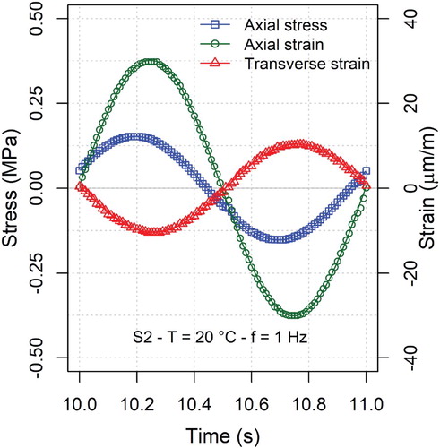
Considering the last ten loading cycles, the periodic component of the measured stress and strain signals was isolated using a moving average filter and approximated with Fourier polynomials, using a least squares regression (Figure 1). The first harmonic component (fundamental harmonic) of the measured axial stress (${\sigma }_1^{\ast }={\sigma }_{1,0}\cdot \exp \left[\text{j}\left(\omega t+{\delta }_1\right)\right]$), axial strain (${\epsilon }_1^{\ast }={\epsilon }_{1,0}\cdot \exp \left(\text{j}\omega t\right)$) and transverse strain (${\epsilon }_2^{\ast }={\epsilon }_{2,0}\cdot \exp \left[\text{j}\left(\omega \tau -{\delta }_2\right)\right]$) were used to calculate the complex Young's modulus $E^{\ast }$ and the complex Poisson's ratio ${\nu }^{\ast }$: (4) $E^{\ast }\left(\text{j}\omega \right)=\frac{{\sigma }_{1,0}}{{\epsilon }_{1,0}}\exp \left(\text{j}{\delta }_1\right)=E_0\exp \left(\text{j}{\delta }_E\right)$(4) (5) ${\nu }^{\ast }\left(\text{j}\omega \right)=-\frac{{\epsilon }_{2,0}}{{\epsilon }_{1,0}}\exp \left(-\text{j}{\delta }_2\right)={\nu }_0\exp \left(-\text{j}{\delta }_{\nu }\right)$(5) where $\text{j}$ is the imaginary unit, $\omega =2\pi f$ is the angular frequency, $E_0={\sigma }_{1,0}/{\epsilon }_{1,0}$ and ${\nu }_0={\epsilon }_{2,0}/{\epsilon }_{1,0}$ are the absolute values, ${\delta }_E={\delta }_1$ and ${\delta }_{\nu }={\delta }_2-\pi$ are the phase angles. Following this sign convention, values ${\delta }_{\nu }>0$ are obtained when the transverse strain lags the axial strain because of viscous effects. Note that Equations (4) and (5) are formally identical to Equation (2).

Figure 1. Example of the sinusoidal stress and strain waveforms measured on specimen S2 at 20°C, f = 1 Hz.

Thermo-rheological modelling

The values of $E^{\ast }$ and ${\nu }^{\ast }$ measured with sinusoidal tests are fitted applying the TTSP principle and using the 2S2P1D LVE model (Olard & Di Benedetto, 2003). The 2S2P1D model features a linear spring in parallel with the series arrangement of a linear spring, two fractional derivative elements (also called parabolic dashpots) and a linear dashpot. The general model equation can be written as follows: (6) $H\left(\text{j}\omega \right)=H_e+\frac{H_g-H_e}{1+d_H{\left(\text{j}\omega {\tau }_H\right)}^{-k_H}+{\left(\text{j}\omega {\tau }_H\right)}^{-h_H}+{\left(\text{j}\omega {\tau }_H{\beta }_H\right)}^{-1}}$(6) where $H\left(\text{j}\omega \right)$ is the complex domain response function ($E^{\ast }$ or ${\nu }^{\ast }$), $H_e$ and $H_g$ are the equilibrium (low frequency) and glassy (high frequency) asymptotic values of $H\left(\text{j}\omega \right)$. The dimensionless constants $k_H$, $h_H$ and $d_H$ represent the response of the two fractional derivative elements and the dimensionless constant ${\beta }_H$ represents the response of the linear dashpot. Using the TTSP, the characteristic time ${\tau }_H$ can be expressed as a function of temperature as follows: (7) ${\tau }_H\left(T\right)=a_R\left(T\right)\cdot {\tau }_{H,R}$(7) where ${\tau }_{H,R}$ is the characteristic time and $a_R\left(T\right)$ are the temperature shift factors, at the chosen reference temperature. In this study, the reference temperature is $T_R$ = 20°C and the values of $a_R\left(T\right)$ are calculated with the closed form shifting (CFS) algorithm (Gergesova, Zupančič, Saprunov, & Emri, 2011). Specifically, the optimal shifting is found by requiring that the area of the overlapping window between two successive isothermal curves of the stiffness modulus $E_0$ is zero. The same shift factors are used for $E^{\ast }$ and ${\nu }^{\ast }$ (Di Benedetto et al., 2007; Perraton et al., 2016) and their temperature dependence is modelled with the Williams-Landel-Ferry (WLF) equation (Williams, Landel, & Ferry, 1955): (8) $\log a_R\left(T\right)=\frac{-C_1\left(T-T_R\right)}{C_2+\left(T-T_R\right)}$(8) where $T_R$ is the reference temperature and $C_1$, $C_2$ are fitting constants.

The 2S2P1D model was extended to describe the 3-dimensional behaviour of bituminous mixtures using the values of the parameters $k_H$, $h_H$, $d_H$ and ${\beta }_H$ optimised for $E^{\ast }$ also for modelling ${\nu }^{\ast }$ (Di Benedetto et al., 2007). In this study, in order to improve the precision of the 2S2P1D model fitting, two completely independent set of parameters ($H_e$, $H_g$, $k_H$, $h_H$, $d_H$, ${\beta }_H$ and ${\tau }_{H,R}$) were optimised for $E^{\ast }$ and ${\nu }^{\ast }$.

Random wave testing

The random wave testing phase was carried out after completing the sinusoidal testing phase. Multi-frequency axial stress waves were applied at 10, 20 and 30°C. Pseudo-random stress waveforms ${\sigma }_1^r\left(t\right)$ were generated using a custom algorithm: (9) ${\sigma }_1^r\left(t\right)=2{\sigma }_{1,0}^r\sum _k\left[\left(r_k-0.5\right)\left(u\left(t-k{T}_f\right)-u\left(t-\left(k+1\right)T_f\right)\right)\right]$(9) where ${\sigma }_{1,0}^r$ is a prefixed stress value, $r_k$ is a random number generated according to the uniform distribution $U\left(0,1\right)$, and $u\left(t\right)$ is the unit step function. Equation (9) is similar to the constant-switching-pace symmetric random signal described by Marmarelis (1977) and defines a stepwise function, where the duration of each step is $T_f=0.02\text{s}$ and the stress values of each step is obtained as the product of ${\sigma }_{1,0}^r$ and $r_k$. 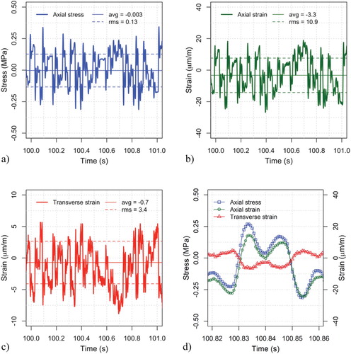For each random test, ${\sigma }_{1,0}^r$ was chosen equal to the amplitude of the sinusoidal stress previously applied on the same specimen at the frequency of 1 Hz and producing a sinusoidal axial strain with amplitude ${\epsilon }_{1,0}$ of 30 μm/m. Three random testing repetitions, with a duration of 120 s, were applied at each temperature. Figure 2 shows an example of the applied random stress waveform and the corresponding measurements of axial and transverse strain. Note the similarity between Figure 2(d), depicting 0.04 s of the random test and Figure 1, depicting 1.0 s of sinusoidal test (the stress and strains were plotted using the same scale).

Figure 2. Example of the random stress and strain waveforms measured on specimen S2 at 20°C (replicate 1): (a) axial stress; (b) axial strain; (c) transverse strain; (d) detail with superposition of stress and strains.

The spectral analysis for the calculation of the FRF was implemented in MATLAB. First, the discrete Fourier transform of the measured stress and strain signals was calculated using the function fft (fast Fourier transform algorithm). Then, the function spafdr was used to estimate the spectrum of the stress and strain signals and the FRF for complex Young's modulus and Poisson's ratio: (10) $E_r^{\ast }\left(\text{j}\omega \right)=\frac{{\mathrm{\Phi }}_{\epsilon 1\sigma 1}\left(\text{j}\omega \right)}{{\mathrm{\Phi }}_{\epsilon 1}\left(\text{j}\omega \right)}$(10) (11) ${\nu }_r^{\ast }\left(\text{j}\omega \right)=-\frac{{\mathrm{\Phi }}_{\epsilon 1\epsilon 2}\left(\text{j}\omega \right)}{{\mathrm{\Phi }}_{\epsilon 1}\left(\text{j}\omega \right)}$(11)

Note that Equations (10) and (11) are formally identical to Equation (3). The function spafdr calculates the spectrum and the FRF in 100 logarithmically spaced frequency points, using the Blackman-Tuckey approach (Ljung, 2018). Finally, the function bode is used to calculate the absolute value and the phase of the FRF at each frequency.

As an example, Figure 3 shows the amplitude spectrum of the stress and strain signals reported in Figure 2. Note that the frequency band of the signals is comprised between f_min = 0.0083 Hz (the reciprocal of the random test duration) and f_max = 800 Hz (one half the sampling frequency used for data acquisition, i.e. the Nyquist frequency). The spectrum of a “purely” random signal (white noise) is expected to have the same amplitude at all frequencies. The amplitude spectrum of the stress wave produced by the press (Figure 3(a)) depends on the algorithm used to generate the pseudo-random wave and on the performance of the servo-hydraulic loading actuator. Here, frequencies higher than 80 Hz may be considered as disturbances, since this is the maximum working frequency of the servo-valve. On the other hand, frequencies in the lower part of the spectrum correspond to excitations with periods comparable to the test duration. Therefore, at these frequencies transient effects may be present in the material response.

Figure 3. Amplitude spectrum of signals plotted in Figure 2: (a) stress; (b) strains.

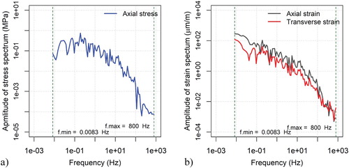
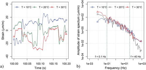
Figure 4(a) shows an example (excerpt from 100.0 s to 100.2 s) of the random axial strain waveforms measured on specimens S2 at 10, 20 and 30°C, whereas Figure 4(b) shows the corresponding amplitude spectrum. It can be observed that the strain levels applied at different temperatures are comparable. Moreover, it can be observed that in the frequency band comprised between 0.1 and 40 Hz the amplitude of the strain spectrum decreases from about 90 μm/m to 1 μm/m. This is different from sinusoidal testing where a fixed strain level is normally applied.

Figure 4. Example of random axial strain measured at 10, 20 and 30°C (specimen S2 replicate 1): (a) time-domain waveforms; (b) amplitude spectrums.

Results and discussion

Sinusoidal testing

Complex Young's modulus

Figure 5 shows the values of $E^{\ast }$ measured with sinusoidal testing in the Cole–Cole and in the Black diagrams. The plots in Figure 5(a and b) compare the results obtained from specimen S1 and S2 at the axial strain level 30 μm/m, while the plots in Figure 5(c and d) compare the results obtained from specimen S2 at 15, 30 and 60 μm/m. The continuous lines superposed to the measured data represent the fitted 2S2P1D models, whose parameters are summarised in Table 1. Figure 6 shows all the calculated shift factors and the fitted WLF model.

Figure 5. Complex Young's modulus measured with sinusoidal tests at different strain levels and 2S2P1D model simulations: (a) Cole-Cole diagram for specimens S1 and S2 at 30 μm/m; (b) Black diagram for specimens S1 and S2 at 30 μm/m; (c) Cole-Cole diagram for specimen S2; (d) Black diagram for specimen S2.

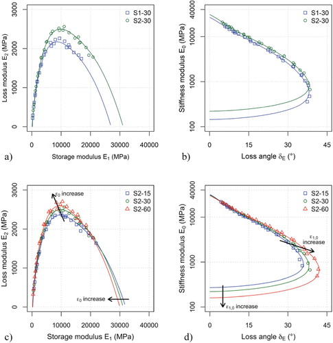
Table 1. Parameters of the 2S2P1D model (T_R = 20°C) for complex Young's modulus measured with sinusoidal testing.

ID	Strain μm/m	Ee MPa	Eg MPa	kE	hE	dE	Log βE	Log τE
S1	60	110	26,000	0.162	0.495	1.780	2.130	−1.471
S1	30	145	27,000	0.159	0.490	2.080	2.200	−1.317
S1	15	160	28,000	0.154	0.482	2.275	2.306	−1.173
S1	0^a	185	28,536	0.152	0.467	2.205	2.130	−0.649
S2	60	160	30,000	0.167	0.515	2.012	1.848	−0.894
S2	30	220	31,117	0.159	0.495	2.100	1.976	−0.787
S2	15	270	32,000	0.146	0.476	2.158	2.060	−0.692
S2	0^a	321	32,591	0.143	0.480	2.459	2.343	−1.110

^a Extrapolated values (see Figure 7).

As can be observed, the $E^{\ast }$ values measured at different temperatures and frequencies follow unique curves in both the Cole–Cole and the Black diagrams. This confirms the accuracy of the measurements and, as expected, validates the application of the TTSP. The values of the stiffness modulus $E_0$ measured on specimen S2 are slightly higher than those measured on specimen S1. This trend is confirmed by the parameters $E_e$ and $E_g$ and is due to the lower air voids content of specimen S2. The values of ${\delta }_E$ measured on both specimens are similar and comprised between 5° and 41°.

The results clearly show that, even at axial strain levels as small as 15 μm/m, the values of $E^{\ast }$ are strain dependent and highlights the effect of nonlinearity. The arrows superposed to the plots in Figure 5(c and d) indicate the change of $E^{\ast }$ due to increasing strain level: a reduction of $E_0$ and an increase of ${\delta }_E$. As a combination of these effects, in Figure 5(c) we observe a reduction of the storage modulus (real part of $E_0$) and an increase of the loss modulus (imaginary part of $E_0$). These results fully confirm the finding of recent studies on nonlinearity of bituminous mixtures that the assumption of LVE behaviour for bituminous mixtures should be considered only as an approximation (Gauthier, Bodin, Chailleux, & Gallet, 2010; Mangiafico et al., 2018; Underwood & Kim, 2012). However, using the LVE approach to describe the material behaviour still provides results that can be used to tackle most practical problems.

Following the last consideration, an attempt was made to analyse the nonlinearity of $E^{\ast }$ by using the 2S2P1D model. To this aim, in Figure 7 the model parameters were plotted as a function of the axial strain level. As can be observed, increasing the strain level from 15 to 60 μm/m leads to a decrease of $E_e$ and $E_g$, which are the constants of the two springs (2S) of the model. This is consistent with the reduction of the $E_0$ values highlighted above. Concurrently, $h_E$ and $k_E$ increase. These parameters represent the order of derivation of the parabolic dashpots, which varies between 0 (purely elastic behaviour) and 1 (purely viscous behaviour). Thus, the increase of $h_E$ and $k_E$ indicates that higher strain levels favour the loss component of the material response versus the reversible component. This is also consistent with the increase of the ${\delta }_E$ values highlighted above. Increasing the strain level, we also observe a decrease of the characteristic time ${\tau }_{H,20}$ (note that in Figure 7 this is shown as an increase of $\text{--}\log \tau$). This confirms that the loss, non-reversible, part of the material response is extended by higher strain levels.

Figure 6. Shift factors obtained from sinusoidal and random testing using the CFS algorithm.

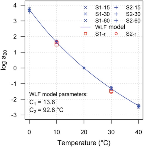
Figure 7. Graphical representation of the 2S2P1D model parameters as a function of the sinusoidal strain level with exponential regression models.

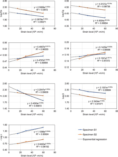
In Figure 7 an exponential function was used to fit the data. This allowed to extrapolate the 2S2P1D parameters for the infinitesimal strain level ${\epsilon }_{1,0}$ = 0 μm/m (Table 1), corresponding to the theoretical “pure” LVE behaviour. The trend of the extrapolated model will be further discussed in the section focused on the results of the random tests.

Complex Poisson's ratio

Figure 8 shows the values of ${\nu }^{\ast }$ measured with sinusoidal testing in the Cole–Cole and in the Black diagrams. The plots in Figure 8(a and b) compare the results obtained from specimen S1 and S2 at the axial strain level 30 μm/m, while the plots in Figure 8(c and d) compare the results obtained from specimen S1 at 15, 30 and 60 μm/m. The continuous lines superposed to the measured data represent the fitted 2S2P1D models, whose parameters are summarised in Table 2.

Figure 8. Complex PR measured with sinusoidal tests at different strain levels and 2S2P1D model simulations: (a) Cole-Cole diagram for specimens S1 and S2 at 30 μm/m; (b) Black diagram for specimens S1 and S2 at 30 μm/m; (c) Cole-Cole diagram for specimen S1; (d) Black diagram for specimen S1.

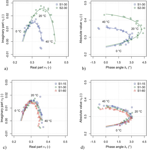
Table 2. Parameters of the 2S2P1D model (T_R = 20°C) for complex Poisson's ratio measured with sinusoidal testing.

ID	Strain μm/m	${\nu }_e$	${\nu }_g$	kv	hv	dv	Log βv	Log τv
S1	60	0.351	0.244	0.330	0.625	4.300	2.600	0.211
S1	30	0.357	0.242	0.285	0.708	2.650	2.450	−0.088
S1	15	0.365	0.237	0.275	0.678	2.850	2.550	0.228
S2	60	0.434	0.247	0.275	0.580	1.950	2.000	0.268
S2	30	0.435	0.247	0.280	0.689	2.100	2.000	0.330
S2	15	0.459	0.249	0.273	0.610	3.400	2.000	1.472

Similar to $E^{\ast }$, the ${\nu }^{\ast }$ values measured at different temperatures and frequencies follow unique curves in both the Cole–Cole and the Black diagrams (Pham et al., 2015). Although the dispersion of the measured data is higher with respect to $E^{\ast }$, the accuracy of the measurements and the validity of the TTSP is confirmed.

At low temperature, the values of ${\nu }_0$ measured on the two specimens are very similar. The average value of ${\nu }_g$ is 0.2410 and 0.2477 for specimens S1 and S2, respectively (less than 3% difference). At high temperature, specimen S2 shows values of ${\nu }_0$ noticeably higher than specimen S1. The average difference between ${\nu }_e-{\nu }_g$ is 0.1167 and 0.1950 for specimens S1 and S2, respectively (almost 70% difference). The values of ${\delta }_{\nu }$ are small, less than 5°, and at high temperature show a change in sign, which is normally found in this parameter at high temperature measurements (Graziani et al., 2018).

Similar to $E^{\ast }$, the results show that the axial strain level has an effect on ${\nu }^{\ast }$. However, this effect is partially masked by the measurement noise. In fact, the amplitude of the measured transverse strain is very small, less than 5 μm/m, which corresponds to a change of the specimen diameter of 1.5 μm and the phase difference of 1° corresponds to a delay of 0.27 ms. Although the nonlinearity of the three-dimensional material response appears reasonable, the precision of the experimental results does not allow to quantify this effect.

Random wave testing

Complex Young's modulus

Figure 9 shows the absolute value and the phase angle of the FRF $E_r^{\ast }$ calculated in 100 logarithmically spaced frequency points from 0.0084–400 Hz. The plots refer to specimen S2, with 3 repetitions at each temperature. The effects of noise are particularly evident in the lower and upper parts of the spectrum, however, in the central part, the signal-to-noise ratio is high enough to observe and quantify the material response.

Figure 9. Raw FRF estimate for the complex Young's modulus (3 replicates for specimen S2).

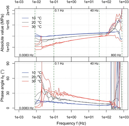
Figure 10 presents the values of $E_r^{\ast }$ in the frequency band comprised between 0.1 and 40 Hz where the 3 replicate measurements show good repeatability and thus allow to calculate the average response using the real and imaginary parts of the signals. The plots in Figure 10(a and b) show average isothermal measurements of the stiffness modulus and loss angle for specimen S2. The trend of the isothermal curves is analogous to the one observed in sinusoidal testing and reveals the usual temperature and frequency dependence of the stiffness modulus and the phase angle. The plots in Figure 10(c and d) compare the results obtained from specimen S1 and S2 in the Cole–Cole and in the Black diagrams. As can be observed, the $E_r^{\ast }$ values measured at different temperatures and frequencies follow unique curves in both diagrams, confirming the consistency of the random wave approach and further validating the TTSP. The discrepancies observed in Figure 10(c and d) may be explained considering that the $E_r^{\ast }$ values measured at constant temperature are not related to a single axial strain level, like in sinusoidal tests, but to an interval of axial strain amplitudes comprised between 1 μm/m (at 40 Hz) and 90 μm/m (at 1 Hz) (Figure 4(b)).

Figure 10. FRF estimate for the complex Young's modulus (average of 3 repetitions from 0.1 Hz to 40 Hz): (a) Isothermal values of stiffness modulus for specimen S2; (b) Isothermal values of loss angle for specimen S2; (c) Cole-Cole diagram for specimens S1 and S2; (d) Black diagram for specimens S1 and S2.

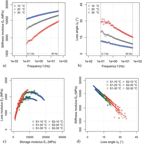
Figure 11 presents the direct comparison between the sinusoidal and the random wave testing results using master curves of the stiffness modulus and phase angle. The results of sinusoidal testing at 15, 30 and 60 μm/m are simulated using the 2S2P1D model and the extrapolated model at 0 μm/m is also depicted. The isothermal values of $E_r^{\ast }$ are shifted using the CFS algorithm. The shift factors are plotted in Figure 6 and are lower than those obtained for sinusoidal testing; the discrepancy is very small and thus it may be due to the precision of the measurements. Indeed, a difference between the values of the characteristic times obtained from tension-compression and dynamic measurements was also observed by Carret, Pedraza, et al. (2018).

Figure 11. Comparison of complex Young's modulus master curves from sinusoidal and FRF from random wave testing (specimen S2): (a) Stiffness modulus; (b) Loss angle.

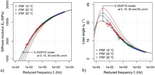
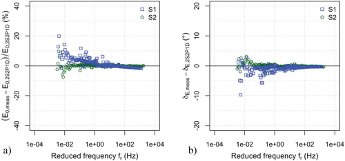
At all reduced frequencies, the stiffness modulus measured with random waves was slightly higher than the sinusoidal measurements, whereas the phase angle was slightly lower. A similar behaviour was observed by Carret, Di Benedetto, et al. (2018), Carret, Pedraza, et al. (2018) Gudmarsson, Ryden, Di Benedetto, et al. (2014) and by Gudmarsson et al. (2015) when comparing the results of sinusoidal tests and dynamic test. In Figure 11, there is a good match between the FRF measurements and the 2S2P1D model at 0 μm/m. This match was further verified by plotting the normalised differences between simulated and experimental values for stiffness modulus (Figure 12(a)) and differences between simulated and experimental values for the phase angle (Figure 12(b)). As can be observed, discrepancies are generally lower than 10% for stiffness modulus (lower than 5% at higher reduced frequencies) and lower than 5° for phase angle (lower than 2° at higher reduced frequencies). The difference between sinusoidal and random test results is probably due to small nonlinearity of the material response and shows that random testing is a powerful tool to estimate the “pure” LVE response of the material.

Figure 12. Difference between experimental results of random testing and simulated values from 2S2P1D model at “0” strain: (a) Stiffness modulus; (b) Loss angle.

Complex Poisson's ratio

Figure 13 shows the absolute value and the phase angle of the FRF ${\nu }_r^{\ast }$. Similar to $E_r^{\ast }$, the values are originally calculated from 0.0084–400 Hz, then the frequencies with a low signal-to-noise ratio (lower and upper parts of the spectrum) are removed and finally the average of three random loading repetitions is calculated. In this case, the frequency band ensuring repeatable results is comprised between 1 Hz and 90 Hz.

Figure 13. Complex PR FRF estimate (average of 3 repetitions, from 1 Hz to 90 Hz): (a) Isothermal values of absolute value for specimen S1; (b) Isothermal values of phase angle for specimen S1; (c) Cole-Cole diagram for specimens S1 and S2; (d) Black diagram for specimens S1 and S2.

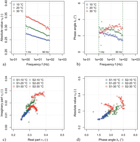
The plots in Figure 13(a and b) show the average isothermal measurements of the absolute value and phase angle of ${\nu }_r^{\ast }$ for specimen S1. Within the selected frequency band, the absolute value measured at constant temperature shows very clear trends. For phase angle data, the signal-to-noise ratio is lower, but reasonable trends can be identified as demonstrated by the interpolating lines obtained with a low-pass filter. The plots in Figure 13(c and d) compare the results obtained from specimen S1 and S2 in the Cole–Cole and in the Black diagrams. At 10°C, the values of ${\nu }_0$ for the two specimens are very similar, whereas at 30°C specimen S2 shows values of ${\nu }_0$ noticeably higher than specimen S1. For both specimens, the values of ${\delta }_{\nu }$ are comprised between 1.5° and 4.5°.

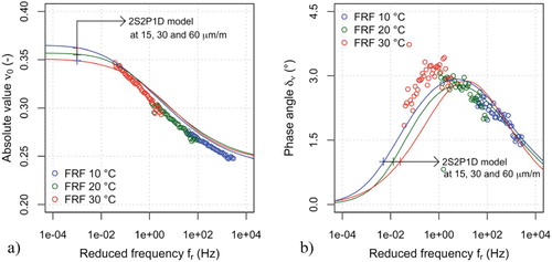
Figure 14 directly compares the sinusoidal and the random wave testing results using master curves of the absolute value and the phase angle. The results of sinusoidal testing at 15, 30 and 60 μm/m are simulated using the 2S2P1D model, while isothermal values of ${\nu }_r^{\ast }$ are shifted using the shift factors previously calculated for $E_r^{\ast }$ (Figure 6). The results show that there is a good superposition between the isothermal measurements of both the absolute value and the phase angle data and thus validate the TTSP. At all reduced frequencies, the absolute value of ${\nu }_r^{\ast }$ is slightly lower than the sinusoidal measurements (maximum difference is about 0.01), whereas the phase angle is slightly higher (maximum difference is about 0.3°). These discrepancies are extremely low if compared, for example, with those obtained by Gudmarsson, Ryden, & Birgisson (2014) and Gudmarsson et al. (2015) using impact resonance testing, which again confirms the accuracy of the random wave testing approach. Although it is tempting to speculate that the discrepancies between the results of sinusoidal and random tests are linked to the material nonlinearity, the precision of the Poisson's ratio data does not allow to draw such a conclusion.

Figure 14. Comparison of complex Poisson's ratio master curves from sinusoidal and FRF from random wave testing (specimen S1): (a) Absolute value; (b) Phase angle.

Conclusion

This study shows a methodology to measure the complex Young's modulus and the complex Poisson's ratio of bituminous mixtures using a multi-frequency mechanical loading. A random axial stress wave is applied to a cylindrical specimen and the corresponding axial and transverse strains are measured. The frequency response functions of the specimen are calculated comparing input and output signals with a spectral analysis approach. Applying 120 s random waves at 10, 20 and 30°C gives results with a high signal-to-noise ratio in the frequency band between 0.1 Hz and 40 Hz for the complex Young's modulus and between 1 and 90 Hz for the complex Poisson's ratio. For both functions the results validate the time-temperature superposition principle. Conventional sinusoidal tests carried out with 15, 30 and 60 μm/m axial strain amplitudes are used as a reference to evaluate the reliability of the random wave approach. The sinusoidal tests show the strain dependency of the material functions confirming that, even at small strain levels, the material behaviour deviates from the rigorous LVE theory. Notwithstanding this deviation, the 2S2P1D rheological model is able to simulate the material response at the adopted strain levels and its parameters can be used to extrapolate the response at infinitesimal strain. Thus, the proposed random loading methodology is an effective tool to estimate the “pure” LVE response of bituminous mixtures.

In conclusion, random wave testing can be carried out with a simple software update to a standard testing press and the data analysis does not require any numerical modelling. This results is a promising alternative to the classical sinusoidal testing procedure. Moreover, as regards fatigue testing, the random wave approach can be used to study the damage evolution over a wide range of frequencies with a single test repetition. This could lead to a significant saving in testing time and material with respect to conventional “single frequency” tests.

Conflict of interest

None.

References

- Airey, G. D., Rahimzadeh, B., & Collop, A. C. (2003). Viscoelastic linearity limits for bituminous materials. Materials and Structures, 36(10), 643–647. doi: 10.1007/BF02479495
- Carret, J. C., Di Benedetto, H., & Sauzeat, C. (2018). Multi modal dynamic linear viscoelastic back analysis for asphalt mixes. Journal of Nondestructive Evaluation, 37(2), 35. doi: 10.1007/s10921-018-0491-3
- Carret, J. C., Pedraza, A., Di Benedetto, H., & Sauzeat, C. (2018). Comparison of the 3-dim linear viscoelastic behavior of asphalt mixes determined with tension-compression and dynamic tests. Construction and Building Materials, 174, 529–536. doi: 10.1016/j.conbuildmat.2018.04.156
- Di Benedetto, H., Delaporte, B., & Sauzéat, C. (2007). Three-dimensional linear behavior of bituminous materials: Experiments and modeling. International Journal of Geomechanics, 7(2), 149–157. doi: 10.1061/(ASCE)1532-3641(2007)7:2(149)
- Di Benedetto, H., Nguyen, Q. T., & Sauzéat, C. (2011). Nonlinearity, heating, fatigue and thixotropy during cyclic loading of asphalt mixtures. Road Materials and Pavement Design, 12(1), 129–158. doi: 10.1080/14680629.2011.9690356
- Di Benedetto, H., Partl, M. N., Francken, L., & Saint André, C. D. L. R. (2001). Stiffness testing for bituminous mixtures. Materials and Structures, 34(2), 66–70. doi: 10.1007/BF02481553
- Gauthier, G., Bodin, D., Chailleux, E., & Gallet, T. (2010). Non linearity in bituminous materials during cyclic tests. Road Materials and Pavement Design, 11(Supp1.), 379–410. doi: 10.1080/14680629.2010.9690339
- Gergesova, M., Zupančič, B., Saprunov, I., & Emri, I. (2011). The closed form tTP shifting (CFS) algorithm. Journal of Rheology, 55(1), 1–16. doi: 10.1122/1.3503529
- Graziani, A., Bocci, E., & Canestrari, F. (2014a). Bulk and shear characterization of bituminous mixtures in the linear viscoelastic domain. Mechanics of Time-Dependent Materials, 18(3), 527–554. doi: 10.1007/s11043-014-9240-x
- Graziani, A., Bocci, M., & Canestrari, F. (2014b). Complex Poisson’s ratio of bituminous mixtures: Measurement and modeling. Materials and Structures, 47(7), 1131–1148. doi: 10.1617/s11527-013-0117-2
- Graziani, A., Cardone, F., & Virgili, A. (2016). Characterization of the three-dimensional linear viscoelastic behavior of asphalt concrete mixtures. Construction and Building Materials, 105, 356–364. doi: 10.1016/j.conbuildmat.2015.12.094
- Graziani, A., Di Benedetto, H., Perraton, D., Sauzéat, C., Hofko, B., Nguyen, Q. T., … Falchetto, A. C. (2018). Three-dimensional characterisation of linear viscoelastic properties of bituminous mixtures. In M. Partl, L. Porot, H. Di Benedetto, F. Canestrari, P. Marsac, & G. Tebaldi (Eds.), Testing and characterization of sustainable innovative bituminous materials and systems (pp. 75–125). Cham: Springer.
- Graziani, A., Di Benedetto, H., Perraton, D., Sauzéat, C., Hofko, B., Poulikakos, L. D., & Pouget, S. (2017). Recommendation of RILEM TC 237-SIB on complex Poisson’s ratio characterization of bituminous mixtures. Materials and Structures, 50(2), 142. doi: 10.1617/s11527-017-1008-8
- Gudmarsson, A., Ryden, N., & Birgisson, B. (2014). Observed deviations from isotropic linear viscoelastic behavior of asphalt concrete through modal testing. Construction and Building Materials, 66, 63–71. doi: 10.1016/j.conbuildmat.2014.05.077
- Gudmarsson, A., Ryden, N., Di Benedetto, H., & Sauzéat, C. (2015). Complex modulus and complex Poisson’s ratio from cyclic and dynamic modal testing of asphalt concrete. Construction and Building Materials, 88, 20–31. doi: 10.1016/j.conbuildmat.2015.04.007
- Gudmarsson, A., Ryden, N., Di Benedetto, H., Sauzéat, C., Tapsoba, N., & Birgisson, B. (2014). Comparing linear viscoelastic properties of asphalt concrete measured by laboratory seismic and tension–compression tests. Journal of Nondestructive Evaluation, 33(4), 571–582. doi: 10.1007/s10921-014-0253-9
- Huang, S. C., & Di Benedetto, H. (Eds.). (2015). Advances in asphalt materials: Road and pavement construction. Cambridge: Woodhead Publishing.
- Kim, Y. R. (2008). Modeling of asphalt concrete. New York, NY: McGraw Hill Professional.
- Larcher, N., Takarli, M., Angellier, N., Petit, C., & Sebbah, H. (2015). Towards a viscoelastic mechanical characterization of asphalt materials by ultrasonic measurements. Materials and Structures, 48(5), 1377–1388. doi: 10.1617/s11527-013-0240-0
- Ljung, L. (1987). System identification: Theory for the user. Upper Saddle River, NJ: Prentice Hall.
- Ljung, L. (2018). MATLAB system identification toolbox: User’s guide. MathWorks Incorporated.
- Mangiafico, S., Babadopulos, L. F. A. L., Sauzéat, C., & Di Benedetto, H. (2018). Nonlinearity of bituminous mixtures. Mechanics of Time-Dependent Materials, 22(1), 29–49. doi: 10.1007/s11043-017-9350-3
- Marmarelis, V. Z. (1977). A family of quasi-white random signals and its optimal use in biological system identification. Biological Cybernetics, 27(1), 49–56. doi: 10.1007/BF00357710
- Mounier, D., Di Benedetto, H., & Sauzéat, C. (2012). Determination of bituminous mixtures linear properties using ultrasonic wave propagation. Construction and Building Materials, 36, 638–647. doi: 10.1016/j.conbuildmat.2012.04.136
- Olard, F., & Di Benedetto, H. (2003). General “2S2P1D” model and relation between the linear viscoelastic behaviours of bituminous binders and mixes. Road Materials and Pavement Design, 4(2), 185–224.
- Oppenheim, A. V., Willsky, A. S., & Nawab, S. H. (1983). Signals and systems (Vols. 2). Englewood Cliffs, NJ: Prentice-Hall, 6(7), 10.
- Perraton, D., Di Benedetto, H., Sauzéat, C., Hofko, B., Graziani, A., Nguyen, Q. T., … Grenfell, J. (2016). 3Dim experimental investigation of linear viscoelastic properties of bituminous mixtures. Materials and Structures, 49(11), 4813–4829. doi: 10.1617/s11527-016-0827-3
- Pham, N. H., Sauzéat, C., Di Benedetto, H., González-León, J. A., Barreto, G., Nicolaï, A., & Jakubowski, M. (2015). Analysis and modeling of 3D complex modulus tests on hot and warm bituminous mixtures. Mechanics of Time-Dependent Materials, 19(2), 167–186. doi: 10.1007/s11043-015-9258-8
- Tschoegl, N. W. (1989). The phenomenological theory of linear viscoelastic behavior: An introduction. Springer Science & Business Media. Viscoelasticity–a critical review. Mechanics of Time-Dependent Materials, 6(1), 3–51. doi: 10.1023/A:1014411503170
- Underwood, B. S., & Kim, Y. R. (2012). Comprehensive evaluation of small strain viscoelastic behavior of asphalt concrete. Journal of Testing and Evaluation, 40(4), 622–632. doi: 10.1520/JTE104521
- Uzan, J., & Levenberg, E. (2007). Advanced testing and characterization of asphalt concrete materials in tension. International Journal of Geomechanics, 7(2), 158–165. doi: 10.1061/(ASCE)1532-3641(2007)7:2(158)
- Virgili, A., Canestrari, F., & Graziani, A. (2013, September 2–4). An experimental approach to the rheological characterization of bituminous mixtures based on pseudo-random stress excitations. Proceedings of the 7th RILEM international conference on Self-compacting Concrete and 1st RILEM international conference on Rheology and Processing of Construction Materials, Paris, France.
- Williams, M. L., Landel, R. F., & Ferry, J. D. (1955). The temperature dependence of relaxation mechanisms in amorphous polymers and other glass-forming liquids. Journal of the American Chemical Society, 77(14), 3701–3707. doi: 10.1021/ja01619a008