Modelling the response of large-size subbase materials tested under varying moisture conditions in a heavy vehicle simulator

Abstract

Pavement design methods must be able to predict the behaviour of pavement materials at increased moisture levels due to climate changes causing increased precipitation and more intense rainfall events. This paper intends to examine the influence of moisture and gradation on pavement response. An instrumented accelerated pavement test (APT) has been conducted on two thin flexible pavement structures with unbound base course and subbase materials using a heavy vehicle simulator (HVS). The two pavement structures were identical except for the gradation of the subbase material, where one had a 0/90 mm curve with a controlled fines content, and the other had an open-graded 22/90 mm curve. The APT was conducted using constant dual-wheel loading, and three different groundwater (GW) levels were induced in order to change the moisture content in the structures. The HVS was stopped regularly for carrying out response measurements from the instrumentation. The analysis is focussed on the response of the unbound aggregate layers to varying moisture levels in the pavement structure. The increased GW level causes a substantial increase in rutting. Conflicting results are found regarding the development of stresses and strains throughout the APT. Two models, linear elastic and non-linear elastic, is employed to model the responses from the pavement structures.

Keywords:

• Unbound granular materials
• accelerated pavement testing
• heavy vehicle simulator
• groundwater table
• water content
• pavement response

1. Introduction

Environmental conditions are important inputs to pavement design, combined with traffic load, material choice and layer thicknesses. Climate changes are in many areas expected to lead to increased precipitation and more intense rainfall events (Seneviratne et al., 2012). Such changes will lead to increased moisture within road structures and possible overloading of road drainage systems. Pavement design has traditionally been done using empirical methods, based on long-term experience with similar materials and conditions (ARA Inc., 2004). When climate changes cause a shift towards increased moisture levels, empirical methods can no longer be used to predict pavement performance. A transition from empirical to mechanistic design is needed, and to achieve this, we need to be able to model the behaviour of the pavement structures under all conditions (Erlingsson, 2007; Mamlouk, 2006).

In the Nordic countries, most roads are designed using flexible pavements, with relatively thin hot mix asphalt (HMA) layers above thicker unbound base and subbase providing a substantial part of the bearing capacity. This practice is partly due to the availability of high-quality aggregate resources, making unbound aggregates an affordable solution.

In Norway, local aggregate resources originating from tunnels and road cuts are often utilised in construction projects. Aggregates can be produced and used on-site, reducing transportation costs for raw materials. Due to space and time restrictions at the construction sites, such production requires a simple setup. These restrictions have, combined with experience with frost heave problems caused by excess fines, resulted in a practice where all fine material is sorted out from the large-size aggregates used in the subbase layer, e.g. 22/125 mm or 16/90 mm (Aarstad et al., 2019; Aksnes et al., 2013). Such gradings may resemble those used for waterbound macadam, but requirements for minimum amount of over- and undersize ensure the gradings are open and not single-sized (Horak & Triebel, 1986; Norwegian Public Roads Administration, 2018).

In Sweden, on the other hand, aggregate resources are normally transported in from quarries where the production methods allow for full quality assessment of the products. Here, large-size aggregate materials with controlled fines content are used in the subbase layer, e.g. 0/90 mm.

Water and moisture have a large influence on the performance of pavement materials (Dawson, 2009). As the moisture content increases, the friction between aggregate particles becomes lower, and the resistance to differential particle deformation is reduced, leading to a reduced resilient modulus of unbound aggregates (ARA Inc., 2004; Erlingsson, 2010; Lekarp & Dawson, 1998). The performance of unbound open-graded aggregates have been subject for previous research (e.g. Heydinger et al., 1996; Nguyen Ahn, 2019), but there is a knowledge gap regarding the performance of large-size open-graded aggregates used in pavements.

The aim of the current research is twofold: (a) to examine the effect of gradation on the responses of subbase materials when tested at different groundwater (GW) levels, and (b) to model the responses from pavement structures with open-graded and well-graded subbase materials. Two subbase materials of equal geological composition are tested, one material containing fines, while the other material had lower sieve size 22 mm. Albeit being composed of the same rock type, such materials will have different properties regarding density, void ratio, permeability and stiffness. Depending on gradation, varying groundwater levels result in varying moisture content in the pavement materials also above the groundwater table (GWT); hence, the influence of moisture content on pavement performance can be evaluated (Erlingsson, 2010; Li & Baus, 2005; Saevarsdottir & Erlingsson, 2013).

The specific objectives of the research can be summarised in three hypotheses:

1. The choice between open-graded and well-graded subbase material has no significance for the long-term pavement performance as long as material properties fulfil set requirements

2. An open-graded subbase material is less affected by moisture changes than a well-graded subbase material

3. Existing response models fit better to well-graded materials than open-graded large-size materials

The first hypothesis is formulated on basis of the prerequisites used in the empirical Norwegian pavement design system (Norwegian Public Roads Administration, 2018), where subbase load distribution factors are not affected by gradation. The second hypothesis is based on findings from previous research (ARA Inc., 2004; Cary & Zapata, 2011; Ekblad & Isacsson, 2006) which may be contrary to the first hypothesis. The third hypothesis is based on the knowledge that using coarse, large-size (d ≥ 0 and D ≥ 90 mm) aggregates in pavement structures is uncommon (Fladvad et al., 2017; Fladvad & Ulvik, 2019), and thus has not been a focus in the development of response models for unbound granular materials.

In order to examine the effects in full scale, an accelerated pavement test (APT) using a heavy vehicle simulator (HVS) was chosen. The APT was conducted at the Swedish National Road and Transport Research Institute (VTI) test facility in Linköping, Sweden in 2018–2019.

2. Materials and methods

2.1. Pavement structures

The APT was conducted using a HVS type Mark IV at the VTI full-scale pavement testing facility (Figure 1(a)). The pavement structures were constructed in a concrete test pit which is 3 m deep, 5 m wide and 15 m long (Figure 1(b)). In the test pit, GWT can be controlled and adjusted.

Figure 1. Heavy vehicle simulator.

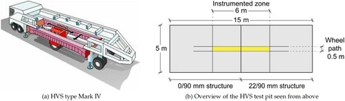
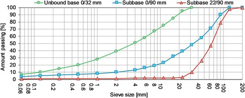
Two pavement structures were tested simultaneously (Figure 1(b)) in order to investigate the difference between an open-graded and a well-graded subbase. Both structures were constructed in the same test pit, each part with a length of 7.5 m. The subbase gradations 0/90 mm and 22/90 mm were chosen; otherwise, the pavement structures were constructed of identical materials. The surface course and bituminous base course were constructed from conventional dense-graded asphalt concrete (AC), where the surface course had upper aggregate size 16 mm and pen 70/100 binder. The bituminous base course had upper aggregate size 22 mm and pen 160/220 binder to ensure good fatigue life properties. Unbound base course (0/32 mm) and subbase were constructed from crushed rock. Particle size distribution curves for the unbound materials are shown in Figure 2. The subgrade consisted of silty sand.

Figure 2. Particle size distribution curves for the unbound pavement materials.

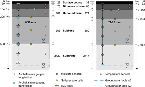
Layer thicknesses for the full pavement structures are shown in Figure 3. The difference in layer thickness between the two structures is due to practical adjustments in the construction process, such as differences in compaction. Due to the geometry of the test pit, the unbound materials were installed partly manually as the test pit could not be accessed by full-size construction equipment normally used to install large-size materials. The unbound materials were compacted until they met requirements for static plate load tests given by Norwegian Public Roads Administration (2018), thus ensuring that the designed stiffness of the materials was achieved. The AC was placed in the test pit using conventional paving equipment.

Figure 3. Cross-section of the pavement structures with vertical distribution of sensors. Layer thicknesses and depth below surface specified in mm. Size of sensors and horizontal distance between sensors not to scale. AC – asphalt concrete layers; UB – Unbound base; Sb – Subbase; Sg – Subgrade.

The subbase materials are supplied from a tunnel construction site in the construction project E39 Svegatjørn–Rådal south of Bergen, Norway. The materials fulfil requirements for subbase materials (Norwegian Public Roads Administration, 2018) regarding gradation, fines content and physical properties. The aggregates have a mixed metamorphic origin, as the tunnels pass through several rock types with unclear transitions between them (Bertelsen, 2014). The open-graded material was selected from the ongoing production at the construction site, while the well-graded material was created by mixing 22/90 and 0/32 mm material at a 1:1 weight ratio.

2.2. Accelerated pavement test

2.2.1. Heavy vehicle simulator

In the main test, the HVS was set up with a dual-wheel configuration. Two 295/80R22.5 tyres were used with a wheel spacing of 34 cm centre-to-centre. The dual-wheel load during testing was 60 kN, corresponding to a 120 kN axle load, and the tyre pressure was 800 kPa. The lateral wander of the wheel was ±25 cm in 5 cm increments, following a normal distribution.

Before the main test started, a pre-loading phase with lower load was applied in order to post-compact the structure. For the initial 20 000 load repetitions, a single 425/65R22.5 wheel was used with a load of 30 kN (axle load 60 kN) and tyre pressure 700 kPa. In this phase, the load was evenly distributed over the wheel path, ±35 cm in 5 cm increments.

All traffic load was applied with bidirectional loading at a constant rolling speed of 12 km/h. A climate chamber was installed to keep the temperature constant at 10 °C.

2.2.2. Groundwater table

The APT was divided into three phases, each with a separate depth of the GWT. GWT was raised by gently pumping water at low velocity through holes in the upper part of the walls in the concrete pit. In phase w1, GWT was located at great depth, > 3 m below the pavement surface. GWT was stable at this level for the first 550 000 load repetitions. For phase w2, GWT was raised to 30 cm below the formation level, corresponding to the depth of the drainage level of a pavement structure in operation. GWT was stable at this level for 368 000 load repetitions. For phase w3, GWT was raised further to a level of about 5 cm above the formation level. This level simulates a situation where the drainage system is overloaded and unable to keep the GWT at the designed drainage level. GWT was stable at this level for 286 000 load repetitions. No traffic load was applied while GWT was raised. GWT depth for phases w2 and w3 are shown in Figure 3.

2.2.3. Instrumentation

Both pavement structures were instrumented using asphalt strain gauges (ASG), soil pressure cells (SPC), strain measuring units (εMU) and moisture and temperature sensors. Each structure was instrumented with three sets of ASGs, two sets of SPCs and εMUs and one set of moisture and temperature sensors vertically distributed as shown in Figure 3. Additionally, the surface rut profile was measured using a laser and straight edge setup.

The instrumentation is described in detail by Saevarsdottir et al. (2016), who used the same test facility and similar equipment. ASGs measure the longitudinal and transversal strain at the bottom of the AC layers. SPCs measuring vertical stress are distributed at the top, middle and bottom of the subbase. εMUs measure vertical strain at 7 different levels; over the bound base layer, unbound base layer, subbase divided between three sensors and two sensors in the subgrade, the lowest reaching to approximately 30 cm below the formation level. Moisture content was measured at four different levels; in the subgrade approximately 15 cm below the formation level, at two levels in the subbase layer, and in the middle of the base layer.

A transition zone was implemented to avoid influence between measurements in the two subbase layers; soil pressure cells were placed 0.8 and 1.7 m from the interface between the structures, and subbase strain measuring units were placed 1.25 and 2.5 m from the interface. Moisture sensors were placed 2.9 m from the interface.

The pavement response was measured nine times during the test, and permanent deformations was measured 13 times, as shown in Table 1. Moisture content was registered continuously.

Table 1. Overview of response measurements during APT.

Phase	Number of load repetitions	Permanent deformation	Full response measurement
w1	0	X
	20 000	X	X
	31 000	X
	80 000	X
	130 000	X	X
	180 000	X
	377 000	X	X
	500 000	X	X
w2	555 000	X	X
	930 000	X	X
w3	940 000	X	X
	1 102 000	X	X
	1 233 000	X	X

2.2.4. Surface measurements

Measurements using falling weight deflectometer (FWD) was conducted before the accelerated traffic started (w1) and at the end of phases w2 and w3. FWD tests were conducted with a 300 mm diameter load plate at loads 30, 50 and 65 kN.

The surface rut profile was measured using a laser which registers the surface cross-section by 250 measurements over 2.5 m width. Three profiles are registered for each structure. Laser profiles were measured on average once per 24 000 load repetitions. In the presentation of rut depth values and profiles, the measured rut depth is corrected for the surface variations measured before any traffic load was applied. Average rut depth is calculated as average over the middle 200 mm of the rut profile (average of 20 individual measurements).

2.3. Modelling

2.3.1. Stiffness of unbound materials

The resilient modulus $M_r$ is a common characteristic of the stiffness of unbound materials, as defined in Equation (1(1) $\begin{array}{rl}{M}_r& =\frac{{\sigma }_d}{{ϵ}_r}\end{array}$(1) ), where ${ϵ}_r$ is the resilient (recoverable) strain in the material under the deviatoric stress ${\sigma }_d$ (Equation (2(2) $\begin{array}{rl}{\sigma }_d& =\sqrt{\frac{1}{2}\left({\left({\sigma }_1-{\sigma }_2\right)}^2+{\left({\sigma }_1-{\sigma }_3\right)}^2+{\left({\sigma }_2-{\sigma }_3\right)}^2\right)}\end{array}$(2) )). A stiffer material shows less strain under a certain load and thus has a higher $M_r$. (1) $\begin{array}{rl}{M}_r& =\frac{{\sigma }_d}{{ϵ}_r}\end{array}$(1) (2) $\begin{array}{rl}{\sigma }_d& =\sqrt{\frac{1}{2}\left({\left({\sigma }_1-{\sigma }_2\right)}^2+{\left({\sigma }_1-{\sigma }_3\right)}^2+{\left({\sigma }_2-{\sigma }_3\right)}^2\right)}\end{array}$(2) When ${\sigma }_2={\sigma }_3$, such as in a repeated load triaxial test, Equation (2(2) $\begin{array}{rl}{\sigma }_d& =\sqrt{\frac{1}{2}\left({\left({\sigma }_1-{\sigma }_2\right)}^2+{\left({\sigma }_1-{\sigma }_3\right)}^2+{\left({\sigma }_2-{\sigma }_3\right)}^2\right)}\end{array}$(2) ) is simplified to ${\sigma }_d={\sigma }_1-{\sigma }_3$.

For stress-dependent materials, the resilient modulus $M_r$ can be calculated from the mean normal stress level using the non-linear elastic k–θ model defined in Equation (3(3) $M_r=k_1{p}_a{\left(\frac{\theta }{p_a}\right)}^{k_2}$(3) ) (Hicks & Monismith, 1971; Uzan, 1985). (3) $M_r=k_1{p}_a{\left(\frac{\theta }{p_a}\right)}^{k_2}$(3) where

• θ bulk stress; $\theta =\frac{{\sigma }_1+{\sigma }_2+{\sigma }_3}{3}$;

• p_a reference pressure (100 kPa)

• k₁; k₂ experimentally determined constants

In the research presented in this paper, the pavement structures' response behaviour is modelled using multi-layer elastic theory (MLET) in an axisymmetrical system using the ERAPave software (Ahmed & Erlingsson, 2012; Erlingsson & Ahmed, 2013) to find the appropriate material properties for the unbound pavement materials. ERAPave is used to calculate both linear elastic and non-linear elastic material behaviour.

2.3.2. Moisture dependency

Increasing moisture content results in a decreasing $M_r$ (Lekarp et al., 2000). The variation in $M_r$ depending on moisture can be expressed by Equation (4(4) ${\log }_{10}\left(\frac{M_r}{M_{r_{opt}}}\right)=a+\frac{b-a}{1+\exp \left(\ln \left(-{\displaystyle \frac{b}{a}}\right)+k_m\left(S-S_{opt}\right)\right)}$(4) ) given in the mechanistic-empirical pavement design guide (MEPDG) (ARA Inc., 2004). Degree of saturation S can be calculated from the water content and porosity of the material. (4) ${\log }_{10}\left(\frac{M_r}{M_{r_{opt}}}\right)=a+\frac{b-a}{1+\exp \left(\ln \left(-{\displaystyle \frac{b}{a}}\right)+k_m\left(S-S_{opt}\right)\right)}$(4) where

• S_opt degree of saturation at a reference condition

• M_ropt resilient modulus at a reference condition

• a minimum of ${\log }_{10}\left(\frac{M_r}{M_{r_{opt}}}\right)$

• b maximum of ${\log }_{10}\left(\frac{M_r}{M_{r_{opt}}}\right)$

• k_m regression parameter

The calibrated MEPDG $M_r$-moisture model shows that coarse-grained materials are less affected by a change in S than fine-grained materials. Due to the large upper size of the subbase materials used in the current research, optimum water content or saturation could not be measured, and established relations regarding variations in $M_r$ as a function of saturation (Equation (4(4) ${\log }_{10}\left(\frac{M_r}{M_{r_{opt}}}\right)=a+\frac{b-a}{1+\exp \left(\ln \left(-{\displaystyle \frac{b}{a}}\right)+k_m\left(S-S_{opt}\right)\right)}$(4) )) could not be used directly. Due to these constraints, $M_r$ is back-calculated from measurements.

The moisture content measured as volumetric water content $w_{vol}$ is defined in Equation (5(5) $w_{vol}=\frac{V_w}{V_{tot}}$(5) ), where $V_w$ is the volume of water and $V_{tot}$ is the total volume of the material including voids. (5) $w_{vol}=\frac{V_w}{V_{tot}}$(5) Gravimetric moisture content $w_c$ can be calculated from $w_{vol}$ by Equation (6(6) $w_c=\frac{{\gamma }_{water}}{\gamma }{w}_{vol}$(6) ), using the unit weight of water (${\gamma }_{water}$) and soil (γ). (6) $w_c=\frac{{\gamma }_{water}}{\gamma }{w}_{vol}$(6)

2.3.3. Temperature dependency

Knowing the AC stiffness $E_{T_{ref}}$ at a reference temperature $T_{ref}$, the stiffness $E_T$ at a temperature T can be calculated from Equation (7(7) $E_T=E_{T_{ref}}{e}^{-b(T-T_{ref})}$(7) ) (Erlingsson, 2012). For the AC material used in this experiment, $E_{T_{ref}}$ is 6500 MPa at 10°C, and the material constant b is assumed to be 0.065. (7) $E_T=E_{T_{ref}}{e}^{-b(T-T_{ref})}$(7)

2.3.4. FWD back-calculation and viscoelasticity

FWD results are back-calculated based on layer thicknesses, moisture content and measured deflection using the ERAPave software. In the software, a single axle/single wheel configuration is used with axle load = 2x FWD load.

AC materials show a general viscoelastic behaviour where strain decreases under a fixed load level if the load frequency is increased (Kim, 2011). This behaviour means that the material appears stiffer when a wheel load is applied at a higher speed. As HVS loading is applied at 12 km/h while the FWD load pulse replicates a wheel load at 70–80 km/h, AC stiffness must be reduced when back-calculated values from FWD tests are used in a linear elastic model of the behaviour from HVS loading (Ahmed & Erlingsson, 2017). Comparison between measured and modelled tensile strain at the bottom of AC layers can be used as an indicator of the fit of the reduced stiffness.

3. Measurements

3.1. Water content

Volumetric water content ($w_{vol}$) was registered continuously throughout the test (Figure 4). In the unbound base, $w_{vol}$ is constant at about 7.3% for both structures in phase w1. In phase w2, $w_{vol}$ remains constant in the 22/90 mm structure, while it increases to 8.6% in the 0/90 mm structure. This increase is finished about one month after GWT is stable at the new level. In phase w3, both structures reach a final $w_{vol}$ of 10.0%. Again, this increase takes about one month in the 0/90 mm structure. In the 22/90 mm structure, on the other hand, the increase from about 7.3% to 9.9% takes place over about 100 days.

Figure 4. Development of volumetric water content ($w_{vol}$) as a function of time for all moisture sensors. Start and end of ground water adjustment periods indicated by vertical dashed lines.

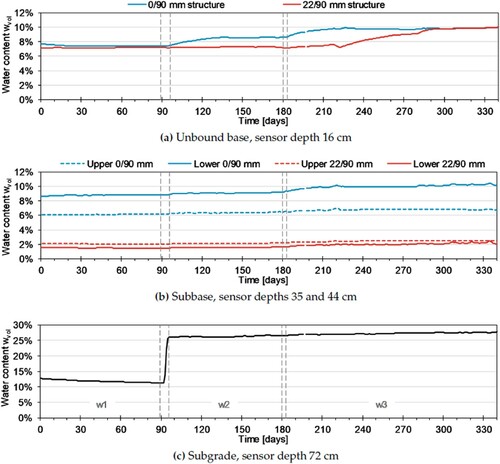
The 22/90 mm crushed rock subbase shows a limited capacity of storing moisture, as $w_{vol}$ starts at 1.5−2.0% in phase w1 and only increases to 2.0−2.5% in the end of phase w3. For this material, the highest $w_{vol}$ is registered by the sensor located at the higher level in the structure. For the 0/90 mm crushed rock material, the tendency is opposite, the lower sensor registers $w_{vol}$ from 8.8% in phase w1 via 9.1% (w2) to 10.3% in phase w3, while the upper sensor spans from 6.1% to 6.8%.

In the subgrade, the registrations show a decreasing tendency in phase w1, likely caused by drainage of water added during compaction of the structures. From the end of phase w1 to the beginning of phase w2 the increase in $w_{vol}$ is very rapid from 11.4% to 26.0%. The difference between phase w2 and w3 is about 1%, showing that the subgrade is almost fully saturated already in phase w2, even though GWT is located about 15 cm below the moisture sensor at this time.

Water content at the time of FWD measurements for all three phases is shown in Table 2, corresponding to day 0, 180 and 338 in Figure 4.

Table 2. Volumetric water content ($w_{vol}$) in unbound base, subbase and subgrade at the time of FWD tests.

	Volumetric water content [%]
	0/90 mm structure			22/90 mm structure
Layer	w1	w2	w3	w1	w2	w3
Unbound base	7.7	8.6	10.0	7.1	7.2	10.0
Subbase, upper	6.1	6.5	6.7	2.1	2.2	2.5
Subbase, lower	8.6	9.2	10.2	1.5	1.6	2.1
Subgrade	12.8	26.6	27.7	12.8	26.6	27.7

Overall, the moisture sensor registrations show that the water content even far above the actual GWT is affected by the raised GWT. The open-graded subbase material does transport moisture vertically, although it takes much longer time than in the well-graded subbase. In the end, $w_{vol}$ in unbound base stabilizes at the same level for both structures, indicating that $w_{vol}$ has reached equilibrium.

3.2. Vertical strain

Figure 5 displays the development of induced vertical strain measured by εMUs in all unbound layers throughout the APT. The measurements are made when the dual wheel is in the centre position, axle load is 120 kN, and tyre pressure is 800 kPa.

Figure 5. Development of induced vertical strain in the unbound materials. Vertical dashed lines indicate GWT raise.

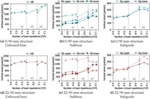
In the unbound base and subbase, the strain increases gradually throughout each phase, while it decreases immediately at each GWT raise. The subgrade shows opposite behaviour; the strain increases immediately after each GWT raise. Comparing strain levels at the end of each GW phase, there is a clear increase as GWT is raised in base and subbase for the 0/90 mm structure. The same is not evident for the 22/90 mm structure, where the behaviour varies between sensors and some sensors show decreased strain at the highest GWT level.

Figure 6 shows the measured strain from all εMU sensors in the unbound layers at the end of each phase (average values from two sensors at each level). The general trend is that the strain level increases throughout the APT as the GWT is raised. In the subgrade, the majority of the increase happens between phase w1 and w2, while there is little change between phase w2 and w3, corresponding well to the registered $w_{vol}$. The subbase and unbound base show a more gradual increase between the phases in the 0/90 mm structure. The 22/90 mm structure shows a gradual increase in strain in the bottom part of the subbase, and also an increase between phase w1 and w2 for the rest of the subbase. Between phase w2 and w3, on the other hand, the strain decreases in the unbound base and the topmost sensor in the subbase.

Figure 6. Measured induced vertical strain at the end of each groundwater level. Horizontal lines indicate layer boundaries.

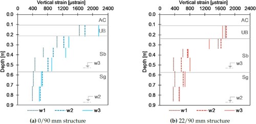
In general, the raised GWT leads to a raised vertical strain level in the structures, even though it does not happen as an immediate change when the GWT is raised. The behaviour differs between the two structures, with the 0/90 mm structure showing the most clear trends of increasing strain.

3.3. Tensile strain

Figure 7 summarises the development of tensile strain in the transversal and longitudinal direction at the lower edge of the AC layers, where the transversal strain is the average from three sensors, while longitudinal strain is the average from two sensors. These measurements are made when the dual wheel is in position −15, meaning that one of the wheels passes directly over the sensor. Axle load is 120 kN, and tyre pressure is 800 kPa.

Figure 7. Development of transversal and longitudinal strain at the bottom of the AC layers. Vertical dashed lines indicate GWT raise.

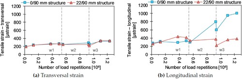
The data shows a trend similar to the vertical strain in the upper parts of the structures – the tensile strain increases gradually within each phase as traffic load is added, while the strain levels decrease immediately after GWT is raised. The transversal strain is at a similar level for both structures, within ± 5% for all measurements except for the last measurement in w2 (930 000 load repetitions) and the first measurement in w3 (940 000 load repetitions), where the transversal strain in the 0/90 mm structure is 17% higher than the 22/90 mm structure.

For longitudinal strain, both structures show the same level for the initial two measurements, but then strain in the 22/90 mm structure increases, and the strain is 25% higher in the 22/90 mm structure at the end of phase w1. This trend changes at the end of phase w2 and all through phase w3, as the longitudinal strain in the 0/90 mm structure is double of the 22/90 mm structure at the end of phase w2, and 170% higher at the end of phase w3. This major increase in longitudinal strain was not expected, neither was the large difference between the structures. Both longitudinal ASG sensors show the same tendency for the 0/90 mm structure, hence the large strain values cannot be interpreted as a measurement error.

3.4. Stress

Figure 8 shows the development of stress registrations in the subbases throughout the APT. The measurements are made when the dual wheel is in the centre position (sensor location between the wheels), axle load is 120 kN, and tyre pressure is 800 kPa.

Figure 8. Development of induced vertical stress during APT. Registrations from three levels in the subbase layers. Vertical dashed lines indicate GWT raises.

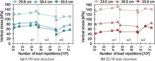
Some post-compaction is seen in phase w1, as the stress increases gradually in both structures. The stress decreases immediately after each GWT raise. The stress remains at the same level through phase w2 for the 22/90 mm structure, while it decreases by on average 16% for the 0/90 mm structure. During phase w3, the stress increases in both structures. At the end of the APT, the registered stress in the 22/90 mm structure is on average 23% higher than after 20 000 load repetitions, indicating increased stiffness. The 0/90 mm structure, on the other hand, has an about 8% lower stiffness level after 1 233 000 load repetitions compared to after 20 000 load repetitions. For both structures, this change is largest for the sensors located at the bottom of the subbase layers.

Vertical stress decreases immediately as GWT is raised, indicating the structures are weakened. This may be caused by increased lubrication at the particle contact points, as water tends to agglomerate at the contact points. Meanwhile, vertical stress increases as traffic load is applied, indicating a structural strengthening from post-compaction and rearrangement of particles within the subbase materials. The measurements indicate that the open-graded material gives higher load distribution than the well-graded material, seen from the lower stress registered in the bottom of the subbase despite the stress in the upper part of the subbase was higher.

3.5. Rut development

Figure 9 shows the development of average surface rut during the APT. A post-compaction tendency can be observed from the increased rut development for the first 100 000 load repetitions, before the rut development approaches a linear trend. The 0/90 mm structure obtains a surface rut depth of $19.0\pm 0.5$ mm after 1 233 000 load repetitions, compared to $19.6\pm 0.4$ mm for the 22/90 mm structure. Through phase w1, the rut development is higher in the 22/90 mm structure, while the tendency is opposite through phase w2. In phase w3, the rut development is similar for both structures. Both structures show indications of a slight uplift as GWT is raised, as the rut depth decreases 1–3% before additional traffic load is applied.

Figure 9. Rut development during APT. Each line represents the average of three laser profiles; error bars show max/min of the three measurements. Dashed vertical lines indicate GWT phase transitions.

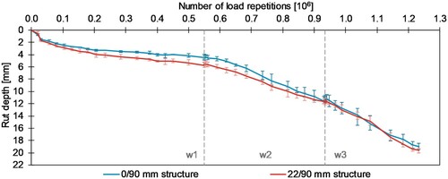
Table 3 lists average rut depth for the middle 200 mm of the cross-section at the end of each groundwater phase, along with the average rutting rate for the final 200 000 load repetitions for each phase. At the end of phases w1 and w3, the rut depth is slightly higher for the 22/90 mm structure, whereas for the end of phase w2, the overall rut depth is similar for both structures. The increasing rutting rate in Table 3 show how the raised GW level in the structure accelerated the plastic deformation rate in individual layers, and, in turn, the rutting rate measured on the surface of the structures. The rutting rate increases by a factor 4.8 from w1 to w2 and by factor 6.1 from w1 to w3 in the 0/90 mm structure. In the 22/90 mm structure, the corresponding numbers are 3.1 and 5.3, showing the influence of a more open subbase gradation.

Table 3. Average rut depth at the end of each groundwater phase and rutting rate for the final 200 000 load repetitions of each phase.

	0/90 mm structure			22/90 mm structure
	w1	w2	w3	w1	w2	w3
Rut depth [mm]	4.50	11.56	19.01	5.73	11.59	19.65
Rutting rate [mm per 100 000 load repetitions]	0.43	2.06	2.64	0.53	1.62	2.84

Both structures show a decreasing rut development towards the end of phase w1, seen from the shape of the w1 development in Figure 9. The same decrease is not seen for phase w2 and w3, but would possibly have occurred had more load repetitions been added to these phases.

4. Response modelling

4.1. Model definitions

Two different approaches are applied to model the responses; a linear elastic (LE) modelling approach using material stiffnesses back-calculated from FWD measurements, and a non-linear elastic (NLE) modelling approach based on Equation (3(3) $M_r=k_1{p}_a{\left(\frac{\theta }{p_a}\right)}^{k_2}$(3) ) fitted to the measured strain levels.

4.1.1. Linear elastic model

Figure 10 shows the FWD deflection and backcalculated deflection bowls from the 50 kN load level. As the climate chamber had to be removed in order to enable FWD measurements, the pavement temperature was not the same for the three measurements. Equation 7(7) $E_T=E_{T_{ref}}{e}^{-b(T-T_{ref})}$(7) shows that the 7.6 °C temperature difference between the measurements results in a 3000 MPa difference in AC stiffness. Hence, the results for w1, w2 and w3 in Figure 10 cannot be compared directly, as the deflection will be too high in w2 and too low in w3 compared to w1. The difference between the structures in each phase is however comparable, showing that although the 22/90 structure gives higher deflection in phase w1, the relation is opposite in w2 and w3. The results indicate that the 0/90 mm structure is more affected by the raised GWT than the 22/90 mm structure. Table 4 shows the backcalculated stiffnesses for each layer with corresponding layer thicknesses. The AC stiffness is backcalculated to 10 °C. The 22/90 mm structure has the lowest stiffness and highest deflection in phase w1, but is less affected by the raised GWT compared to the 0/90 mm structure. It is evident that the raised GWT and increased $w_{vol}$ results in a weakening of the structures through decreased stiffness.

Figure 10. Measured and back-calculated deflection from FWD tests with load 50 kN. Distance from load centre in mm, deflection in μm.

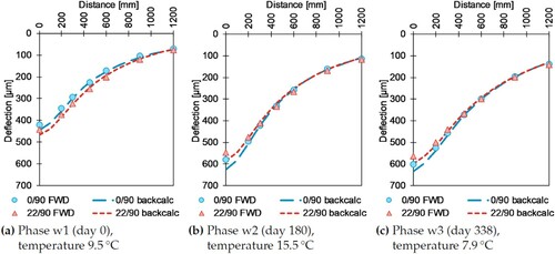
Table 4. Unit weights (γ), layer thicknesses and stiffnesses used in the linear elastic (LE) modelling.

		0/90 mm structure				22/90 mm structure
			Stiffness [MPa]				Stiffness [MPa]
	Unit weight [kN/m^3]	Thickness [mm]	w1	w2	w3	Thickness [mm]	w1	w2	w3
AC layers	24	104	3800	3800	3800	112	3800	3800	3800
Unbound base	20	101	250	225	203	121	250	250	203
Subbase 1	19	163	220	157	149	150	143	143	135
Subbase 2	19	150	220	143	129	150	143	143	135
Subbase 3	19	50	220	129	116	50	143	143	135
Subgrade 1	16	300	82	66	46	300	82	66	46
Subgrade 2	16	2132	82	53	46	2117	82	53	46
Concrete test pit	25	∞	50000	50000	50000	∞	50000	50000	50000

In the modelling of HVS responses, the AC stiffness is reduced from 6500 to 3800 MPa to adjust for the low speed of the HVS (12 km/h) compared to the FWD measurements (Kim, 2011). Poisson's ratio is assumed constant for all materials, $\nu =0.35$. In the back-calculation procedure, the subbase was divided into three sublayers and the subgrade in two sublayers. The division between the sublayers Subgrade 1 and Subgrade 2 mirrors the depth of the GWT in phase w2, while the division between Subbase 2 and Subbase 3 mirrors GWT in phase w3.

From the stiffness values, it appears that the difference in deflection between phase w1 and w2 in the 22/90 mm structure is only due to the decrease in subgrade stiffness. For the 0/90 mm structure, on the other hand, base and subbase stiffness is also affected by the introduction of a raised GWT in phase w2. Between phase w2 and w3, stiffness in all unbound layers is affected in both structures.

4.1.2. Non-linear elastic model

In the NLE model, the unbound base and subbase materials are treated as stress-dependent. To fit the NLE model to the strain measurements, the k–θ model (Equation (3(3) $M_r=k_1{p}_a{\left(\frac{\theta }{p_a}\right)}^{k_2}$(3) )) is used for the stress-dependent layers. AC and subgrade materials are treated as linear elastic in the same way as in the LE model, but with subgrade stiffness deviating from the LE model, as it is fitted to the measured strain. As the temperature during HVS loading was always 10 °C, the AC stiffness is constant but reduced for reduced speed as in the LE model. The NLE model uses the stiffness and $k_1$ values in Table 5 with coefficient $k_2=0.6$. Coefficient $k_1$ varies between layers and moisture levels to fit the measured induced vertical strain from Figure 6. Poisson's ratio is assumed constant for all materials, $\nu =0.35$. In the NLE model, the thickness of sublayers corresponds to the distance between εMU coils.

Table 5. Layer thicknesses, unit weights (γ), stiffnesses and $k_1$ coefficients used in the non-linear elastic (NLE) modelling.

			w1		w2		w3
	Thickness	Unit weight	Stiffness	$k_1$	Stiffness	$k_1$	Stiffness	$k_1$
	[mm]	[kN/m^3]	[MPa]	[ – ]	[MPa]	[ – ]	[MPa]	[ – ]
AC layers	104	24	3800	–	3800	–	3800	–
Unbound base	101	20	–	375	–	340	–	260
Subbase 1	120	19	–	650	–	550	–	500
Subbase 2	103	19	–	950	–	730	–	450
Subbase 3	140	19	–	1700	–	740	–	600
Subgrade	2429	16	82	–	55	–	50	–
Concrete test pit	∞	25	50000	–	50000	–	50000	–
(a) 0/90 mm structure
			w1		w2		w3
	Thickness	Unit weight	Stiffness	$k_1$	Stiffness	$k_1$	Stiffness	$k_1$
	[mm]	[kN/m^3]	[MPa]	[ – ]	[MPa]	[ – ]	[MPa]	[ – ]
AC layers	112	24	3800	–	3800	–	3800	–
Unbound base	121	20	–	340	–	340	–	360
Subbase 1	100	19	–	330	–	310	–	450
Subbase 2	100	19	–	860	–	850	–	650
Subbase 3	150	19	–	1800	–	1100	–	680
Subgrade	2417	16	82	–	55	–	50	–
Concrete test pit	∞	25	50000	–	50000	–	50000	–
(b) 22/90 mm structure

Subgrade stiffness decreases as GWT is raised, showing that the subgrade is weakened. The same is seen from the decreasing $k_1$ values between the GW phases for the stress-sensitive layers. Coefficient $k_1$ decreases for all sublayers except between w2 and w3 for the unbound base and topmost sublayer of the subbase in the 22/90 mm structure. These exceptions are difficult to explain structurally, but originates from the measured strain in Figure 6. Subbase $k_1$ values generally increases with increasing depth.

4.2. Results from modelling

4.2.1. Vertical strain

The fit of the models to the measured vertical strain as a function of depth is shown in Figure 11. The LE model does not provide a good fit to the vertical strain registrations in the unbound base and subbase, as the model predicts too low strain at all GW levels. For the unbound base, the LE model predicts the vertical strain to only 1/3 of the measured strain. For the subbase, the LE model predicts the strain to on average 50% of the measured strain for the 0/90 mm structure, and 60% for the 22/90 mm structure. For both structures, the fit of the LE model is best for phase w1.

Figure 11. Comparison between measured and modelled induced vertical strain as a function of depth at the end of each groundwater phase. Horizontal lines indicate layer boundaries.

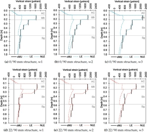
The NLE model is defined by the vertical strain measurements, so naturally, the modelled strain fits very well to the measured strain. An exception is found for the middle part of the subbase in phase w3, where the measurements show a lower strain level in this sublayer than the lowest sublayer. This was considered a measurement error, and the model is fitted with a strain level for this sublayer between the strain levels of the neighbouring sublayers.

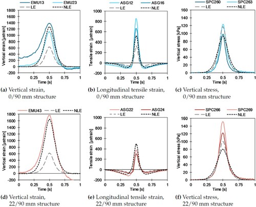
The measured and modelled vertical strain signals as the loading wheel passes over the sensor at a speed of 12 km/h are compared in Figure 12(a,d) for sensors in the top part of the subbase for both structures. The modelled signal is calculated at a depth corresponding to the midpoint of the εMU sensor span. The strain measurements in Figure 11 was made with the dual-wheel load passing directly above the sensors. At the surface above the sensors, the calculation position is located in the centre between the two loading wheels. Data in Figure 12 represents phase w2, similar trends were seen for the two other phases.

Figure 12. Fit of linear elastic (LE) and non-linear elastic (NLE) response models to signals from pavement sensors. Vertical strain in subbase (a, d); longitudinal tensile strain at bottom of AC layers (b, e); vertical strain in subbase (c, f). Data representing phase w2.

4.2.2. Tensile strain

In this section, data for sideposition −15 cm is used, meaning that one of the dual wheels passes directly over the sensors. The fit of the models to the measured tensile strain is shown in Table 6, where the general tendency is that both models calculate a gradual increase in tensile strain. This complies with the measurements from the 0/90 mm structure, but the 22/90 mm structure show a decrease in transversal strain between phase w1 and w2, before the strain increases in phase w3. For longitudinal strain in the 22/90 mm, the measured value decreases from phase w1 to w2, and is constant from phase w2 to w3.

Table 6. Summary of measured (ASG) and modelled (LE, NLE) tensile strain. Δ denotes the difference between measured and modelled values.

		0/90 mm structure					22/90 mm structure
		ASG	LE	Δ	NLE	Δ	ASG	LE	Δ	NLE	Δ
		[$\mu ϵ$]	[$\mu ϵ$]	[%]	[$\mu ϵ$]	[%]	[$\mu ϵ$]	[$\mu ϵ$]	[%]	[$\mu ϵ$]	[%]
Transversal	w1	268	197	−26	308	15	268	199	−26	311	16
	w2	286	220	−23	346	21	248	201	−19	332	34
	w3	327	232	−29	375	15	342	217	−36	335	−2
Longitudinal	w1	329	293	−11	472	44	412	296	−28	475	15
	w2	799	327	−59	525	−34	378	299	−21	500	32
	w3	1007	344	−66	566	−44	378	324	−14	503	33

Another general tendency is that the LE model underestimates the tensile strain while the NLE model overestimates the values. For transversal strain, the fit for each model is similar for both structures, where LE underestimates the strain by on average 26%, and NLE on average overestimates the strain by 16%. For longitudinal strain, neither model replicates the large increase in the 0/90 mm structure. The LE model is closer to the longitudinal strain in the 22/90 mm structure with an average underestimation by 21% opposed to a 27% overestimation by the NLE model.

Measured and modelled longitudinal tensile strain signals at the lower edge of the AC layers are shown in Figure 12(b,e). The signals show the induced tensile strain as the loading wheel passes over the sensor at a speed of 12 km/h.

The higher tensile strain calculated by the NLE model compared to the LE model, matches the vertical strain results in Figure 11, even though the LE model is closer to calculating the tensile strain than the vertical strain. Generally, both models calculate strain in the right order of magnitude, but do not replicate the ASG development between GW phases correctly for the 22/90 mm structure. Neither model can replicate the increase in longitudinal strain for the 0/90 mm structure, which could indicate an ASG measurement error. However, the presented ASG values are averages from two sensors, where both show the same behaviour.

4.2.3. Stress

The fit of the models to the measured vertical stress as a function of depth is shown in Figure 13. Both models calculate a decrease in stress as GWT is raised for both structures, and both models show a larger decrease for the 0/90 mm structure than the 22/90 mm structure. The measured stress does not support such clear trends, especially for the 22/90 mm structure where the lowest stress at all subbase levels is found in phase w2. The LE model calculates a similar decrease in stress for both structures, 9% decrease from w1 to w2 and 15% decrease in total from w1 to w3. The NLE model calculates a somewhat larger stress decrease in the 0/90 mm structure, with 13 and 17% as opposed to 10 and 14% for the 22/90 mm structure. For the 0/90 mm structure, the measurements show a 26% decrease in stress from w1 to w2, but only 19% in total from w1 to w3, meaning the stress increases from w2 to w3. Similarly, the 22/90 mm structure shows a 14% decrease in stress from w1 to w2, but a 2% increase in stress from w1 to w3.

Figure 13. Comparison between measured and modelled induced vertical stress as a function of depth at the end of each groundwater phase. Horizontal lines indicate layer boundaries.

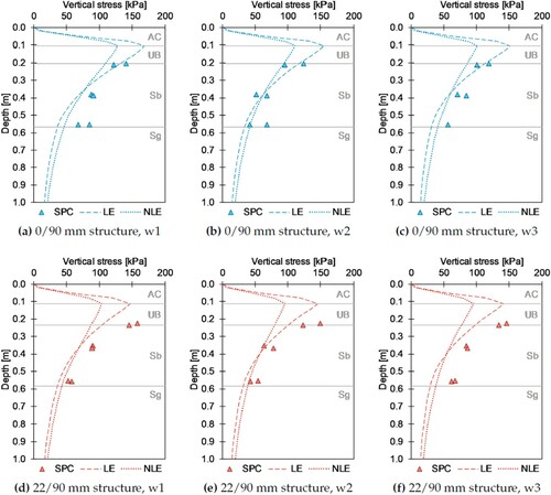
The LE model predicts the lowest stress at the bottom of the subbase, approximately 80% lower than the NLE model. The LE model does, however, calculate a higher rate of change throughout the subbase, resulting in the stress from the LE model being 24% higher than the NLE model at the top of the subbase. These numbers are common for both structures. The rate of change from the LE model fits best to the 22/90 mm structure, although the overall stress level is underestimated for all phases. Both models underestimate the stress, as the LE model predicts on average 81% of the measured stress for the 0/90 mm structure, and 69% for the 22/90 mm structure, based on an average for all three sensors and GW phases. The corresponding numbers for the NLE model are 80% for 0/90 and 69% for 22/90. Hence, both models predict the stress better for the 0/90 mm structure.

The NLE model provides a somewhat better fit to the measured stress level, but neither model replicates the development between phases correctly. The poor fit of the models to the measured stress in the subbase materials makes it difficult to infer any knowledge regarding the stress level in the unbound base and subgrade based on the models.

The stress measurements in Figure 13 was made with the dual-wheel load passing directly above the sensors. At the surface above the sensors, the calculation position is located in the centre between the two loading wheels, hence the modelled stress is zero at the surface.

Figure 12(c,f) display the fit of the modelled vertical stress signal to the signal registered by SPCs as the loading wheel passes over the sensor at a speed of 12 km/h.

5. Discussion

5.1. Accelerated traffic

The accelerated traffic of 1 233 000 load repetitions at 120 kN axle load corresponds to 2.56 million 10 tonne standard axles. Assuming a 10% share of heavy vehicles, this amount of standard axles equals 20 years with annual daily traffic of 3000 vehicles per day on a two-lane road, using the traffic calculation method given by Norwegian Public Roads Administration (2018). The pavement structures in the APT was designed following the guidelines for low-volume roads, and the accelerated traffic corresponds to the amount of load repetitions such a road would experience over a 20 year design period.

A total rut depth of less than 20 mm after 20 years of traffic signals that both structures were durable and did not break down even though groundwater phase w3 was designed to simulate flooding of the drainage system. However, it is important to note that a pavement exposed to regular traffic would be subjected both to temperature fluctuations including freeze/thaw cycles, precipitation and possibly wear from studded tyres which would all increase the rutting. The controlled groundwater variations in this test simulated flooding, but a pavement in operation would be exposed to a much more rapidly fluctuating groundwater table. This may affect the pavement degradation differently than the controlled environment in the APT. However, the controlled environment enables more reliable modelling.

5.2. Water content development following raised groundwater table

The moisture registrations (Figure 4) show that the raised GWT causes $w_{vol}$ to increase far above the new GWT level. Although $w_{vol}$ shows a minimal increase in the 22/90 mm subbase material during the APT, the overlying unbound base reaches the same $w_{vol}$ towards the end of the test as the unbound base above the 0/90 mm subbase. The moisture transport through the 22/90 mm material does, however, take considerably longer time.

The development of $w_{vol}$ shows that the moisture level in the structures was not constant during traffic loading. Still, at the time of FWD measurements, the development was finished, and the FWD results for phase w2 and w3 represents the moisture level at equilibrium. The FWD results are indicators of the performance of the full pavement structures and clearly show that the structures are weakened following both GWT raises. Impact from raised GWT is seen for all types of sensors in the structures, as well as the surface measurements. Salour and Erlingsson (2013) manipulated the drainage system of a road section in operation to change GWT, and measured the response by FWD. They found that the moisture sensors had an extremely quick response to the drainage manipulation, corresponding to the subgrade measurements in the current study. Furthermore, lower stiffness values were back-calculated from FWD tests when GWT increased. The FWD results from the APT agree with these results from a full pavement structure in operation. The Salour & Erlingsson study involved materials with higher fines content and thereby higher moisture contents (15% in subbase) which may explain the more rapid moisture development compared to the APT.

5.3. Conflicting strain vs. stress

Stress measurements show an immediate decrease in stress as GWT is raised (Figure 6), which could be explained as a weakening caused by lubrication of particle contact points. However, both vertical (Figure 5) and tensile (Figure 7) strain sensors show a decrease in strain at the same time as stress decreases, indicating a structural strengthening which does not fit the proposed explanation. The moisture registrations do not support the immediate changes in stresses and strains, particularly in the transition between w2 and w3, where no changes in $w_{vol}$ are seen by the time of the first response measurement in phase w3.

Both types of strain sensors (ASG and εMU) show increased strain as traffic load is applied, indicating a gradual weakening of the structures at the same time as stress sensors show gradually increased stress indicating strengthening. Considering the full APT, vertical strain has increased in the 0/90 mm structure, but this is not evident in the 22/90 mm structure. Longitudinal strain ends at a substantially higher level for the 0/90 mm structure compared to the 22/90 mm structure, while transversal strain remains at a similar level for both structures. The authors are unable to explain these conflicts, and the models show the theoretically expected behaviour, where the increased strain following raised GWT causes the stress levels to decrease. The compliance between εMU and ASG measurements ensure that the strain development is genuine.

5.4. Linear vs. non-linear modelling

The models consider only the stresses and strains measured at the end of each GW phase, and does not involve the immediate changes in stress and strain as GWT is raised. This also means that the models do not consider the developing $w_{vol}$ as traffic load is added. For the theoretical considerations, this fact is a disadvantage. On the other hand, considering a road in operation, traffic load will always be applied evenly even though moisture levels are changing in the structures. The gradually increasing $w_{vol}$ can possibly explain part of the surprisingly linear rut development in the structures during traffic loading.

The LE model underestimates both vertical strain, tensile strain and vertical stress, where the underestimation is highest for the vertical strain. The LE model does, however, provide a better fit to the stress distribution in the 22/90 mm subbase than the NLE model. The poor fit of the LE model shows that the unbound materials should be considered stress sensitive. The NLE model is based on the measured vertical strain, and thus replicates the vertical strain in the unbound layers very well. The NLE model overestimates the tensile strain at the bottom of the AC layers, both longitudinal and transversal, while the vertical stress in the subbases is underestimated.

In the NLE modelling, coefficient $k_1$ and $k_2$ should not be back-calculated simultaneously (Li & Baus, 2005). Coefficient $k_2$ is known to be less or insignificantly affected by moisture (Kolisoja, 1997; Rada & Witczak, 1981; Rahman & Erlingsson, 2016). To isolate the effect of changing moisture levels on $M_r$, coefficient $k_2$ was kept constant at 0.6 for all materials and moisture levels, while coefficient $k_1$ was varied to fit the measured vertical strain. The improved fit of the NLE model to strain rather than stress was also found by Ahmed and Erlingsson (2012). Based on the findings from Ekblad and Isacsson (2006), a higher $k_2$ value should have been used for the open-graded 22/90 mm material, which may have resulted in better compliance between modelled stress and strain for the 22/90 mm structure. Due to the large upper size of the subbase materials used in the current research, the stress and strain behaviour could not be examined using the repeated load triaxial test. Similarly, optimum water content or saturation could not be measured, and established relations regarding variations in $M_r$ as a function of saturation (Equation (4(4) ${\log }_{10}\left(\frac{M_r}{M_{r_{opt}}}\right)=a+\frac{b-a}{1+\exp \left(\ln \left(-{\displaystyle \frac{b}{a}}\right)+k_m\left(S-S_{opt}\right)\right)}$(4) )) could not be used directly.

6. Conclusions

An accelerated pavement test was conducted on two instrumented pavement structures where the moisture conditions were varied through increasing the groundwater table twice. The accelerated traffic applied to the structures corresponds to 20 years with annual daily traffic of 3000 vehicles per day on a two-lane road, assuming heavy vehicles constitute 10% of the total traffic. During the test, the moisture content in unbound materials was monitored continuously, rut depth was measured regularly, and pavement response in the form of stresses and strains was measured at all groundwater levels. The pavement structures were also evaluated using FWD at all groundwater levels.

The APT shows that pavement structures are extremely sensitive to changes in the groundwater level. The increased GWT from w1 to w3 causes the rutting rate to increase by factor 5 for the open-graded structure and factor 6 for the well-graded structure. This means that for each truck that passes the pavement structure, the contribution to permanent deformations are more than five times as big if the drainage system is overloaded so that GWT reaches the bottom of the subbase layer compared to a drained pavement structure. The APT results show that the influence of moisture is far superior to the influence of the difference in gradation between the two structures.

Both structures proved to be durable, showing just short of 20 mm rut depth after 1.23 million load repetitions with axle load 12 tonnes (60 kN dual-wheel load). Neither structure showed any sign of breakdown due to the traffic or flooding. On this general level, hypothesis (1) is confirmed, in that as long as the pavement structure is constructed of strong materials with a controlled fines content and compacted well, the difference in gradation has little impact on the long-term pavement performance.

The APT analysis finds clear differences in the response of the two pavement structures, most notably in their response to the increased GWT. The increase in water content is both lower and slower in the open-graded structure. Both vertical strain and longitudinal tensile strain increases more in the well-graded structure as GWT is raised to the highest level. These findings confirm hypothesis (2), although the effect on the overall structure through accumulated permanent deformations is similar between the structures.

Hypothesis (3) is evaluated based on the models' fit to the two structures. The effect is most clear for the modelling of stress, where both LE and NLE models provide a reasonable fit for the 0/90 mm structure, while both models underestimate the stress level in the 22/90 mm structure. For vertical and tensile strain, the differences between models are more clear than the difference between the models' fit to each structure. Hence, no clear conclusion can be drawn regarding hypothesis (3).

No explanation is found for the contradicting measurements of stress and strain. The measurements are consistent throughout all test phases and for both structures and should be studied further. Another topic for further study is the development of permanent deformations, which should be modelled to investigate the cause of the linear rut development.

Acknowledgments

The research presented here is funded by the Norwegian Public Roads Administration, with contribution from the Research Council of Norway through the industrial innovation project Use of local materials (project no. 256541). The authors would like to thank the construction company Veidekke for supplying the subbase materials to the APT.

This manuscript constitutes a part of the first author's PhD degree at the Department of Geoscience and Petroleum, NTNU – Norwegian University of Science and Technology.

Disclosure statement

No potential conflict of interest was reported by the author(s).

Additional information

Funding

This work was supported by Statens vegvesen.

References

- Aarstad, K., Petersen, B. G., Martinez, C. R., Günther, D., Macias, J., Mathisen, L. U., Fladvad, M., Haugen, M., Nålsund, R., Danielsen, S. W., & Bjøntegaard, Ø. (2019). Local use of rock materials – production and utilization state-of-the-art (1st ed., Tech. Rep.). https://www.sintef.no/globalassets/project/kortreist-stein/012-kortreist-stein-sota-h3-endelig.pdf.
- Ahmed, A. W., & Erlingsson, S. (2012). Modeling of flexible pavement structure behavior-Comparisons with Heavy Vehicle Simulator measurements. In D. Jones, J. Harvey, A. Mateos, & I.L. Al-Qadi (Eds.), Advances in pavement design through full-scale accelerated pavement testing (pp. 493–503). CRC Press.
- Ahmed, A. W., & Erlingsson, S. (2015). Numerical validation of viscoelastic responses of a pavement structure in a full-scale accelerated pavement test. International Journal of Pavement Engineering, 18(1), 47–59. https://doi.org/https://doi.org/10.1080/10298436.2015.1039003
- Aksnes, J., Myhre, Ø., Lindland, T., Berntsen, G., Aursand, P. O., & Evensen, R. (2013). Frost protection of Norwegian Roads. Basis for revision of the Norwegian pavement design manual (Tech. Rep.). Norwegian Public Roads Administration. https://www.vegvesen.no/Fag/Publikasjoner/Publikasjoner/Statens+vegvesens+rapporter/_attachment/748672?.
- ARA Inc. (2004). Guide for the mechanistic-empirical design of new and rehabilitated pavement structures, final report (Tech. Rep. NCHRP 1-37A). Transportation Research Board of the National Academies. http://onlinepubs.trb.org/onlinepubs/archive/mepdg/guide.htm.
- Bertelsen, G. (2014). Geologi – E39 Svegatjørn – Rådal. K10 Svegatjørn – fanavegen (Tech. Rep.). Statens vegvesen Region vest.
- Cary, C. E., & Zapata, C. E. (2011). Resilient modulus for unsaturated unbound materials. Road Materials and Pavement Design, 12(3), 615–638. https://doi.org/https://doi.org/10.1080/14680629.2011.9695263
- Dawson, A. R. (2009). Water in road structures (1st ed., Vol. 5). Springer Netherlands. https://doi.org/https://doi.org/10.1007/978-1-4020-8562-8
- Ekblad, J., & Isacsson, U. (2011). Influence of water on resilient properties of coarse granular materials. Road Materials and Pavement Design, 7(3), 369–404. https://doi.org/https://doi.org/10.1080/14680629.2006.9690043
- Erlingsson, S. (2011). Impact of water on the response and performance of a pavement structure in an accelerated test. Road Materials and Pavement Design, 11(4), 863–880. https://doi.org/https://doi.org/10.1080/14680629.2010.9690310
- Erlingsson, S. (2011). Numerical modelling of thin pavements behaviour in accelerated HVS tests. Road Materials and Pavement Design, 8(4), 719–744. https://doi.org/https://doi.org/10.1080/14680629.2007.9690096
- Erlingsson, S. (2012). Rutting development in a flexible pavement structure. Road Materials and Pavement Design, 13(2), 218–234. https://doi.org/https://doi.org/10.1080/14680629.2012.682383
- Erlingsson, S., & Ahmed, A. W. (2013). Fast layered elastic response program for the analysis of flexible pavement structures. Road Materials and Pavement Design, 14(1), 196–210. https://doi.org/https://doi.org/10.1080/14680629.2012.757558
- Fladvad, M., Aurstad, J., & Wigum, B. J. (2017). Comparison of practice for aggregate use in road construction – results from an international survey. In A. Loizos, I. Al-Qadi, and T. Scarpas (Eds.), Bearing capacity of roads, railways and airfields (pp. 563–570). CRC Press. https://www.taylorfrancis.com/books/e/9781315100333/chapters/https://doi.org/10.1201/9781315100333-74.
- Fladvad, M., & Ulvik, A. (2019). Large-size aggregates for road construction – a review of standard specifications and test methods. In Bulletin of Engineering Geology and the Environment. http://link.springer.com/https://doi.org/10.1007/s10064-019-01683-z.
- Heydinger, A. G., Xie, Q., Randolph, B. W., & Gupta, J. D. (1996). Analysis of resilient modulus of dense- and open-graded aggregates. Transportation Research Record: Journal of the Transportation Research Board, 1547(1), 1–6. https://doi.org/https://doi.org/10.1177/0361198196154700101
- Hicks, R. G., & Monismith, C. L. (1971). Factors influencing the resilient response of granular materials. Highway research record (345). http://onlinepubs.trb.org/Onlinepubs/hrr/1971/345/345-002.pdf.
- Horak, E., & Triebel, R. H. H. (1986). Waterbound macadam as a base and a drainage layer. Transportation Research Record, 1055, 48–51. http://onlinepubs.trb.org/Onlinepubs/trr/1986/1055/1055-006.pdf
- Kim, J. (2011). General viscoelastic solutions for multilayered systems subjected to static and moving loads. Journal of Materials in Civil Engineering, 23(7), 1007–1016. https://doi.org/https://doi.org/10.1061/(ASCE)MT.1943-5533.0000270
- Kolisoja, P. (1997). Resilient deformation characteristics of granular materials(Doctoral dissertation). Tampere University of Technology.
- Lekarp, F., & Dawson, A. R. (1998). Modelling permanent deformation behaviour of unbound granular materials. Construction and Building Materials, 12(1), 9–18. https://doi.org/https://doi.org/10.1016/S0950-0618(97)00078-0
- Lekarp, F., Isacsson, U., & Dawson, A. R. (2000). State of the art. I: Resilient response of unbound aggregates. Journal of Transportation Engineering, 126(1), 66–75. https://doi.org/https://doi.org/10.1061/(ASCE)0733-947X(2000)126:1(66)
- Li, T., & Baus, R. L. (2005). Nonlinear parameters for granular base materials from plate tests. Journal of Geotechnical and Geoenvironmental Engineering, 131(7), 907–913. https://doi.org/https://doi.org/10.1061/(ASCE)1090-0241(2005)131:7(907)
- Mamlouk, M. (2006). Design of flexible pavements. In T. Fwa (Ed.), The handbook of highway engineering (pp. 8–1–8–35). CRC Press.
- Nguyen, T. H., & Ahn, J. (2019). Experimental evaluation of the permanent strains of open-graded aggregate materials. Road Materials and Pavement Design, 1–12. doi:https://doi.org/10.1080/14680629.2019.1702086
- Norwegian Public Roads Administration (2018). Håndbok N200 Vegbygging [Manual N200 Road construction]. Statens vegvesen Vegdirektoratet. https://www.vegvesen.no/_attachment/2364236/binary/1269980.
- Rada, G., & Witczak, M. W. (1981). Comprehensive evaluation of laboratory resilient moduli results for granular material (No. 810). http://onlinepubs.trb.org/Onlinepubs/trr/1981/810/810-004.pdf.
- Rahman, M. S., & Erlingsson, S (2015). Moisture influence on the resilient deformation behaviour of unbound granular materials. International Journal of Pavement Engineering, 17(9), 763–775. https://doi.org/https://doi.org/10.1080/10298436.2015.1019497
- Saevarsdottir, T., & Erlingsson, S. (2013). Water impact on the behaviour of flexible pavement structures in an accelerated test. Road Materials and Pavement Design, 14(2), 256–277. https://doi.org/https://doi.org/10.1080/14680629.2013.779308
- Saevarsdottir, T., Erlingsson, S., & Carlsson, H. (2014). Instrumentation and performance modelling of heavy vehicle simulator tests. International Journal of Pavement Engineering, 17(2), 148–165. https://doi.org/https://doi.org/10.1080/10298436.2014.972957
- Salour, F., & Erlingsson, S. (2013). Moisture-sensitive and stress-dependent behavior of unbound pavement materials from in situ falling weight deflectometer tests. Transportation Research Record, 2335(1), 121–129. https://doi.org/https://doi.org/10.3141/2335-13
- Seneviratne, S., Nicholls, N., Easterling, D., Goodess, C., Kanae, S., Kossin, J., Luo, Y., Marengo, J., McInnes, K., Rahimi, M., Reichstein, M., Sorteberg, A., Vera, C., & Zhang, X. (2012). Changes in climate extremes and their impacts on the natural physical environment. In C. Field, V. Barros, T. F. Stocker, Q. Dahe. (Eds.), Managing the risk of extreme events and disasters to advance climate change adaptation: A special report of working groups I and II of the intergovernmental panel on climatechange (IPCC) (pp. 109–230). Cambridge University Press. https://www.ipcc.ch/site/assets/uploads/2018/03/SREX-Chap3_FINAL-1.pdf.
- Uzan, J (1985). Characterization of granular material. Transportation Research Record, 1022(1), 52–59. http://onlinepubs.trb.org/Onlinepubs/trr/1985/1022/1022-007.pdf.