Design life of rigid pavements under dynamic wheel loads

Abstract

The investigation of the pavement performance under dynamically increased wheel loads combines approaches about the modelling of axle assemblies, the simulation of the dynamic wheel loads due to longitudinal unevenness as well as the estimation of the impact on the service life of pavements. The focus in this work is laid on the determination of distress and service life of rigid pavements under dynamic wheel loads using a recently introduced and for the purpose of this study adopted mechanistic-empirical design method for rigid pavements. The results show a good correlation between the assessed Weighted Longitudinal Profile (WLP) (as an indicator for longitudinal unevenness) and the theoretical service life of rigid pavements. Based on that correlation a rating scheme for longitudinal unevenness is introduced. It allows the classification of the unevennes of roads in a five-grade system depending on the WLP and the definition of limiting values for the longitudinal unevenness.

Keywords:

• dynamic wheel loads
• rigid pavements
• performance
• service life
• longitudinal unevenness
• weighted longitudinal profile

1. Introduction

Since the primary function of a pavement structure is to transfer the repetitive vehicle traffic loads to the subgrade, information about the traffic volume and the composition of the collective of heavy good vehicles is essential in the design process. Thus, in most design approaches the selection of pavement construction depends on the number of vehicles expected to pass the pavement during the intended service life and their overall and axle weights. As design calculations have been computationally expensive for long times, a common method for consideration of the traffic load is to assume a standardised axle weight (usually 80–100 [kN]) which is related to actual vehicle types by damage equivalency factors (ARA, Inc., 1993; FGSV, 2012; FSV, 2016).

Despite the fact that the traffic loads have two components – a static component caused by the vehicle weight over the vehicle axles and a dynamic component caused by the vehicle's motion due to road unevenness – typically only the static one is considered in the pavement design. Previous studies on the interaction between pavement and vehicle (Addis, 1992; Cole & Cebon, 1989; Gyenes & Mitchell, 1992; Rys, 2019; Sun, 2001), have shown that as soon as an unevenness is present, the vehicle starts to oscillate, and this results in dynamically increased wheel and axle loads. These dynamic loads lead to increased distress and accelerated pavement deterioration and thus shorter service life.

A common way to describe the relation between vehicle's axle weight and the change in the pavement damage is the Fourth Power Law (ARA, Inc., 1993). This means that an increase in the wheel load acts on the distress of a pavement approximately with the fourth power (ARA, Inc., 1993). However, it is known that the fourth power law can only be used as a first rough approximation. There are currently several models in place for the assessment of road distress, which calculate Dynamic Load Coefficients (DLC) based on the ratio of dynamic to static wheel load. Some researchers estimated the DLC based on measured wheel loads (Cebon, 1999; Cole & Cebon, 1989; Davis & Bunker, 2011; De Beer & Fisher, 2013; Eisenmann, 1975; Gajda et al., 2018; Hassan, 2012; Mitchell et al., 1992; Mitschke, 1979; Ruiz et al., 2019; Sweatman, 1983). In a more recent study (Harasim & Gajewski, 2021), a correlation between the International Roughness Index (IRI) and the change of the axle loads due to an unevenness on the basis of physical measurements by means of Traffic Speed Deflectometer (TSD) device was derived. Further, they calculated the axle load equivalence factors with the use of the fourth power law for different IRI classes. At class A (0.89 $\left[\mathrm{m}\cdot {\mathrm{k}\mathrm{m}}^{-1}\right]$) the axle load equivalence factors falls in the range of 0.93–1.07 which can be interpreted as 14% range of change to the impact of vehicle load on the durability of pavement due to the level of surface roughness. For rougher roads, the axle load equivalence factor is between 0.73 and 1.34 yielding the range of changes at the level of 61%.

Other researchers focused on development of mathematical models of truck suspension, which allow the simulation of heavy vehicle mainly along a road surface profile and consequently the estimation of the load at the interface between tyre and pavement (Buhari et al., 2013; Gagnon et al., 2015a, 2015b; Park et al., 2014; Sun, 2001, 2013, 2014)

The impact of the dynamic wheel loads on the structural behaviour of pavements has been investigated by several researchers (Cebon, 1999; Khavassefat, 2014; Khavassefat et al., 2015, 2016; Machemehl & Lee, 1974; Ruiz et al., 2019; Rys, 2019; Rys et al., 2016). As the most popular longitudinal unevenness indicator, IRI has been correlated with the pavement response under dynamic wheel loads. Khavassefat et al. (2015) reported that the horizontal stress at the surface and the bottom of an asphalt layer can increase by 50% with a rougher profile (IRI of 2.3 $\left[\mathrm{m}\cdot {\mathrm{k}\mathrm{m}}^{-1}\right]$) in comparison to a smoother profile with IRI of 0.99 $\left[\mathrm{m}\cdot {\mathrm{k}\mathrm{m}}^{-1}\right]$. Bilodeau et al. (2017) compared the service life for the classical static loading and for dynamic loading for three highway flexible pavement structures. When dynamic loads are considered, it was found that the pavement service life may be reduced by about 29 and 20% for bottom-up fatigue cracking and structural rutting failure criteria, respectively. Rys (2019) showed that the dynamic axle loads increase rapidly with pavement evenness deterioration, resulting in up to 25% faster development of pavement distresses for IRI of 4.0 $\left[\mathrm{m}\mathrm{m}\cdot {\mathrm{m}}^{-1}\right]$ and vehicle speed 60–90 $\left[\mathrm{k}\mathrm{m}\cdot {\mathrm{h}}^{-1}\right]$.

Generally, in Europe, three types of unevenness indicators are used, IRI, waveband analysis and the Weighted Longitudinal Profile (WLP). Each one of these has its advantages and limitations (Múčka, 2013, 2015; Rossel-Khavassefat et al., 2022). As identified earlier, IRI is the most popular indicator among others and has been used in the analysis of the impact of dynamic wheel loads on the pavement response, despite the fact that it cannot represent fully the statistical properties of the pavement surface (Múčka, 2015). Further, Rossel-Khavassefat et al. (2022) compared different indicators (among others IRI and WLP) for the longitudinal unevenness with real measured profile data and concluded that there is no strong correlation between them, because these indicators measure different wavelength range, and thus describe different physical phenomena.

The WLP which is well established in the German speaking countries, was developed by Ueckermann and Steinauer (2008) in Germany and than further investigated by Spielhofer et al. (2009) in Austria. Its computation involves three steps: (i) filtering of the measured raw profile to wavelengths of less than 50 m, (ii) weighting of the pre-filtered profile and and (iii) calculation of the standard deviation ${\sigma }_{WLP}$ and the range of variation ${\mathrm{\Delta }}_{WLP}$ that describes the difference between the largest and the smallest value in the examined road section (in Austrian this length of evaluated sections is set to 50 [m]) of the WLP. The WLP is capable of characterising all three phenomena of longitudinal evenness: irregular, periodic and transient unevenness. Compared to other approaches, the WLP method combines the advantages of the response-type methods (implicit evaluation of the shape and size of unevenness with respect to driving dynamics) with those of purely geometrical methods of evaluation (objectivity, without restriction of vibration properties and speed). Previous studies (Kamiya et al., 2012; Spielhofer & Ueckermann, 2012) have indicated that the WLP is not only capable of characterising all phenomena of longitudinal evenness but also that it can differentiate the characteristics of asphalt and concrete pavements. Having all this in mind and considering the fact that ${\mathrm{\Delta }}_{WLP}$ is sensitive to single obstacles, that are the main cause of increased dynamic wheel load, the WLP was chosen as an unevenness indicator for the purpose of this study.

The main objectives of this paper are: (i) to identify dynamic wheel loads (representative for the Austrian highway network), (ii) to consider the dynamic wheel loads in the estimation of the damage and the service life of rigid pavements using the Austrian mechanistic-empirical design method for rigid pavements (Eberhardsteiner et al., 2018) and the WLP, (iii) to develop an evaluation method for longitudinal unevenness that accounts for the structural behaviour of the pavement and enables the assessment of road sections with a concrete pavement.

2. Determination of representative static and dynamic traffic loads

In order to obtain a realistic estimation of wheel loads, these are obtained from empirically derived axle loads of a representative load collective of heavy traffic in Austria, whereby the load spectrum is reproduced with simulation models. A fundamental step here is the consideration of the different truck types from the representative load collective as being composed of axle aggregates.

The description of the representative load collective as well as the derived axle assemblies and static wheel loads can be found in Section 2.1. Section 2.2 describes the modelling process, illustrates the decomposition of a truck model into axle assemblies and justifies various modelling assumptions. The wheel load simulations carried out, the results of which are included in the pavement modelling process, are presented in Section 2.3; here the relationship between dynamic wheel loads and longitudinal unevenness indicators is also discussed.

2.1. Determination of representative static wheel loads

The Austrian pavement design method (Blab et al., 2014; Eberhardsteiner et al., 2016; FSV, 2020) considers specific information about the volume and composition of heavy traffic in the definition of static traffic loads. It takes into account the following parameters: (i) traffic volume of heavy good vehicles (HGV), (ii) the probability of the appearance of HGV types, (iii) the distribution of HGV gross vehicle weights and (iv) the distribution of HGV axle loads. These parameters were defined based on data about the volume of the heavy traffic from records gained in the course of automatic road toll stations and in bridge weigh-in-motion measurements in 2008 on 5 different locations. The analysis of the bridge weigh-in-motion measurements enabled the derivation of characteristic distributions of gross weights and axle loads.

Additionally, using this data, a load collective representative for the heavy traffic on the Austrian motorways and expressways has been established, which includes 12 typical vehicle types with different axle assemblies. The estimation of the traffic loads considers characteristic distributions of vehicle types (Eberhardsteiner et al., 2016), frequencies p of gross weights $G_i$ of vehicle type j and axle loads $A{L}_{ij}$ of axle i of vehicle j, which are representative for the heavy traffic in Austria: (1) $p_{Gj}=g_1\cdot N({\mu }_1,{\sigma }_1)+g_2\cdot N({\mu }_2,{\sigma }_2)$(1) and (2) $A{L}_{ij}={\text{β}}_i+{\alpha }_i\cdot G_i,$(2) where μ and σ are mean value and standard deviation of a standard normal distribution N, while $g_1$ and $g_2$ are weighing factors. As described in Eberhardsteiner et al. (2016) these parameters and ${\text{β}}_i$ and ${\alpha }_i$, have been derived from the bridge weigh-in-motion measurements mentioned above.

To simulate the dynamic wheel loads using the modular approach, trucks were disassembled into their axle assemblies and representative static wheel loads of all axle assemblies (single, tandem and tridem) were defined. These serve as an input data for the simulation of the dynamic wheel loads. After their simulation the vehicles were reassembled to form the 12 representative vehicle types and used as an input parameter in the determination of the distress and service life of the rigid pavement.

2.2. Vehicles modelling

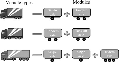
To be able to simulate the dynamic wheel loads occurring when passing an unevenness, the representative vehicle types (trucks) need to be modelled first. In accordance with the outlined methodology, the objective of the simulation was to obtain the best possible model to describe characteristic trucks representative of the load collective and not to simulate a single truck from a particular manufacturer as accurately as possible. Heavy trucks can be considered as modular systems whose individual modules are assembled in a variety of combinations. The modules include axles with different load capacities and bodies with different functions, dimensions and weights, which are connected to each other by standardised spring-damper elements. Therefore, the defined vehicle types from the load collective can be disassembled into their axle assemblies (single, tandem and tridem).

The chosen modular approach is shown schematically in Figure 1. Trucks are represented by two modules – a front one and a rear one. The front one represents the front part of the truck frame, the engine, the cab, the front axle and the part of the load supported on the front axle. The rear module expresses the rear part of the truck frame, the rear axles and the part of the load supported by the rear axles. Trailers and semi-trailers can be represented by the three modules with one, two or three axles. A trailer consists of one or two modules depending on whether it is a conventional trailer with a long wheelbase or a trailer with a tandem axle (Figure 1). This kind of truck representation offers a simple modelling approach of different truck types by adjusting their weight and loading.

Figure 1. Modular representation of vehicle types.

The creation of partial models is based on a 2D spring damper model of a semi-trailer truck that was developed in a previous study (Spielhofer et al., 2013). The developed partial models can be described by common differential equations of second order, in which the wheel loads are calculated (i.e. the vertical pressure occurring in the contact area between tire and road). These are derived from the equations of motion of the mechanical model of the vehicle and are then transformed into a first-order equations to obtain a general state space representation in terms of a time-invariant system. In case of linear parameters, this results in a linear time invariant system (LTI). This form of representation is particularly suitable for the description of a dynamic transmission system, as which the vehicles are regarded.

The simulation is carried out for each assembly by adjusting the load. The parameters of the partial models were derived based on empirical data (Ueckermann & Oeser, 2015).

The modular approach assumes that for the consideration of the vertical contact forces between tire and road the front and rear vehicle parts could be considered decoupled. The reasons for this assumption are that (i) the frame torsional stiffness has practically no influence on the wheel load fluctuations (Zahnmesser et al., 1981 ), (ii) the wheelbase is much larger than the body movement and (iii) the influence of the pitching motion on the wheel load fluctuations is negligible (Mitschke & Wallentowitz, 2004).

The plausibility of the proposed model was confirmed by comparing measured wheel load data on real trucks (Bachmann et al., 2008) with simulated wheel loads. Based on (Ueckermann & Oeser, 2015), the influence of using different modelling approaches such as linear and non-linear damper characteristics or 2D and 3D modelling was also investigated (Spielhofer et al., 2013).

2.3. Simulation of dynamic wheel loads

As described above, input data to the developed models for the simulation of the dynamic wheel loads are the representative static wheel loads and measured longitudinal profile data. For the purpose of this study real longitudinal profile data available in a longitudinal resolution of 10 [cm] from a measurement campaign in 2014 on the entire Austrian motorway network with a total length of approximately 4.259 [km] was used (Spielhofer et al., 2009). As identified in the introduction, the WLP is capable of characterising all phenomena of longitudinal evenness and there is a good correlation between WLP and the dynamic wheel loads. Therefore, it is reasonable to use this roughness indicator to examine the actual effect of unevenness on the road structure.

The longitudinal data for the performed evaluation of the longitudinal evenness was processed according to EN (2006) and was filtered using a band pass filter with cut-off wavelengths from 0.5 to 50 [m]. The tire is taken into account in the simulation using a Butterworth low-pass filter applied to the longitudinal profile. Furthermore, in order to exclude unrealistic dynamic wheel loads as a result of extreme profile variations, such as those at bridge joints, the profile was additionally smoothed. Specifically, segments that have a height difference of more than 3 $\left[\mathrm{c}\mathrm{m}\right]$ in a window of 90 $\left[\mathrm{c}\mathrm{m}\right]$ length are replaced by linearly interpolated sections. Jumps greater than 3 $\left[\mathrm{c}\mathrm{m}\right]$ are obvious to the roadway service and would be quickly eliminated. The window length of 90 $\left[\mathrm{c}\mathrm{m}\right]$ is based on the dimensions of joints. The reason for these jumps could be isolated measurement errors.

The pre-processed longitudinal profiles served as an input for the simulation of the dynamic wheel loads of the modelled axle assemblies. The input signal for the simulation in time domain was from the longitudinal profile on which vehicles are moving with a constant speed of 80 $\left[\mathrm{k}\mathrm{m}\cdot {\mathrm{h}}^{-1}\right]$ (legal speed limit for HGVs in Austria). To determine the occurring dynamic wheel loads on the whole Austrian motorway network, corresponding simulations were carried out for all axle assembly variations with their respective static wheel loads.

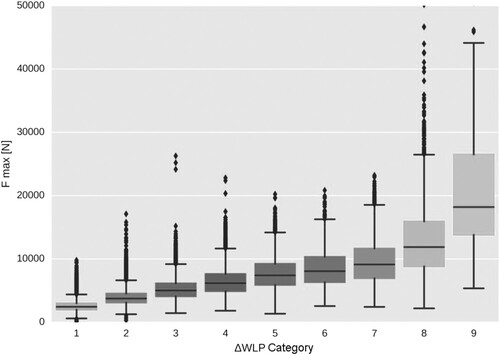
The further processing of the results includes a discretisation of the WLP parameters into nine categories and a corresponding aggregation. The definition of the nine categories, which can be imagined as a histogram, was done under the following aspects: (i) sufficiently fine degree of discretisation in value ranges where many data are available, (ii) sufficiently fine degree of discretisation in value ranges which are relevant for the damage calculation, (iii) sufficiently coarse degree of discretisation to limit the computational effort and to guarantee reliable occupation numbers. Since the first point suggests a rather low and the second point a rather higher number of classes, a meaningful subdivision is not obvious. Therefore, the classification was done iteratively. Figure 2 shows the distribution of the maxima of the dynamic wheel loads in the 9 categories.

Figure 2. Distribution of the maxima of the dynamic wheel loads in the 9 categories.

The results of the simulations are dynamic wheel loads for each point of the longitudinal profile and each axle assembly variation, whereby a connection to local unevenness in the profile can be established. WLP plays an important role in these considerations. In order to establish a correlation between the WLP and the dynamic wheel loads, it has to be considered that the WLP is usually applied in aggregated form, specifically as ${\sigma }_{WLP}$ (the standard deviation of the weighted longitudinal profile in the whole section) and ${\mathrm{\Delta }}_{WLP}$ (the range that describes the difference between the largest and the smallest value of the weighted longitudinal profile in a section) (Spielhofer & Ueckermann, 2012). For these two characteristic values – analogous to IRI characteristic value currently in use in Austria – an evaluation background can be derived. These two characteristic values allow a road network evaluation with regard to evenness.

The dynamic wheel load maxima per category were aggregated using the median. The median was preferred to the average due to its robustness against outliers. Other quantiles are theoretically possible, but since the basis is sectional maxima, this type of averaging seems reasonable. In a further step the ${\mathrm{\Delta }}_{WLP}$ was chosen as an indicator suitable for assessment of the road distress due to unevenness, as ${\mathrm{\Delta }}_{WLP}$ is sensitive to single obstacles, that are the main cause of increased dynamic wheel loads (see Ueckermann & Steinauer, 2008)

3. Determination of distress and service life

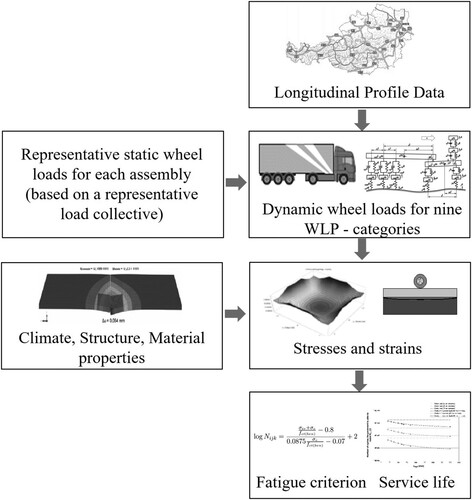
The following chapter presents a brief overview of the recently developed mechanistic-empirical pavement design method for rigid pavements in Austria (Eberhardsteiner et al., 2016, 2018, FSV, 2020). In this work, this method has been adapted in order to analyse and quantify the effects of the dynamic traffic load component caused by the road unevenness, on the structural distress and, thus, the theoretical service life (expressed as number of load cycles the pavement is able to resist, $N_{res}$) of rigid pavement structures (Figure 3).

Figure 3. Flowchart of the procedure for consideration of the dynamic wheel loads in the estimation of the service life of rigid pavements.

3.1. Input parameters to the model

As described above, the traffic loading consists of static and dynamic components. While static wheel loads describe the acting dead loads that occur only on completely even roads, dynamic wheel loads are caused mainly by passing a longitudinal unevenness. A representative load collective of the heavy traffic represents the current static traffic load in Austria. For this composition, actual wheel loads were determined and grouped into representative axle and wheel loads for three axle assemblies (single, tandem and tridem). The dynamic wheel loads were calculated considering the derived representative wheel loads and longitudinal profiles of the Austrian highway network (Figure 3). They are an input parameter for the estimation of the total traffic load and thus for the investigation of the effect of the longitudinal unevenness on distress of rigid pavements.

Another important input parameter is the load transfer in the transverse joints. According to the Austrian standard construction method, the rigid pavements have to be separated by longitudinal and transverse contraction joints. While transverse joints have to be dowelled, longitudinal joints have to be anchored by tie bars especially at heavy traffic load. While dowel bars are responsible for transverse load transfer between adjacent slabs, tie bars have to secure the position of the slabs in transverse direction Foltin et al. (2016). The dowel bar diameter strongly effects the load transfer efficiency and, thus, the pavement performance. Hence, to evaluate the load transfer potential of a dowel, a dowel effectiveness number, DEN, is introduced. DEN is equal to the equivalent stiffness of a vertical spring and can be calculated with the applied load F divided by the resulting vertical deflection w, as shown in equation (3) $DEN=F/w$(3)

The climate and hydrological local conditions have a significant impact on the pavement performance, therefore the seasonal change in the subgrade bearing capacity and the seasonal temperature distribution in the concrete layer are considered in the prediction of the design life. Hence, the various seasonal subgrade conditions are represented by four different values of the subgrade modulus for each season (Table 1) (Litzka et al., 1996).

Table 1. Seasonal bearing capacities.

Layer	E-Modulus [MPa]
Concrete slab	30,000
Asphalt	3500
	P1	P2	P3	P4
Base layer	678	169	242	339
Subgrade	280	70	100	140

Furthermore, the temperature loading correspondingly the temperature distribution in the concrete slab induces stresses that can force the slab to warp upward or downward. In the Austrian design approach these warping stresses are estimated using the Eisenmann-Houben model (Bayraktarova et al., 2017, 2021; Eisenmann & Leykauf, 2003; Houben, 2009), which considers the temperature difference between the top and the bottom or the temperature gradient of the concrete slab. Hence, representative temperature gradients (Table 2) were established using a temperature prediction model and surface temperature data from measuring stations distributed over the Austrian rigid highway network in Bayraktarova et al. (2021).

Table 2. Temperature gradients $\mathrm{\Delta }T$ [K/mm] for the six climate periods (Bayraktarova et al., 2021).

Period 1	Period 2	Period 3	Period 4	Period 5	Period 6
16.12–15.03	16.03–15.05	16.05–15.06	16.06–15.09	16.09–15.10	16.10–15.12
0.023	0.070	0.083	0.076	0.045	0.020

The strength characteristics of the used concrete play a crucial role for the fatigue resistance and thus for the technical service life as result from the design. A dataset of experimental results from bending tensile, splitting tensile and compressive strength tests were analysed in order to derive characteristic relations between different strength properties. To gain characteristic stiffness assumptions, a dataset of experimental results obtained on concrete types typically used in pavements was analysed, resulting in values of concrete Young's modulus between 30,000 and 36,000 $\left[\mathrm{N}\cdot {\mathrm{m}\mathrm{m}}^{-2}\right]$. Hence, the Young's modulus in pavement design is assumed as 30,000 $\left[\mathrm{N}\cdot {\mathrm{m}\mathrm{m}}^{-2}\right]$, the bending tensile strength of the concrete of 5.27 $\left[\mathrm{N}\cdot {\mathrm{m}\mathrm{m}}^{-2}\right]$ and the Poisson ratio is fixed at 0.15.

Considering these input parameters and the slab geometry, the stresses and strains due to temperature and traffic loading can be estimated using the enhanced Eisenmann's model (Houben, 2009) for the curling stresses ${\sigma }_c$ $[N\cdot m{m}^{-2}]$ and the further developed Kirchhoff plate theory method (Höller et al., 2019) for the traffic stresses ${\sigma }_{tr}$ $\left[\mathrm{N}\cdot {\mathrm{m}\mathrm{m}}^{-2}\right]$. Together with the strength properties of the concrete $f_{ct\left(ben\right)}$ $\left[\mathrm{N}\cdot {\mathrm{m}\mathrm{m}}^{-2}\right]$ these stresses are integrated in the Smith's fatigue criterion (Eisenmann & Leykauf, 2003), which allows the estimation of the pavement service life. The allowable number of cycles the pavement is able to resist $N_{ijk}$ for each axle i of each vehicle j and each climate period k are given by (4) $\log N_{ijk}=\frac{\frac{{\sigma }_{tr}+{\sigma }_c}{f_{ct\left(ben\right)}}-0.8}{0.0875\frac{{\sigma }_c}{f_{ct\left(ben\right)}}-0.07}+2$(4) The corresponding damage $C_{ijk}$ is defined as follows (5) $C_{ijk}=\frac{1}{N_{ijk}}.$(5) and the average damage $C_{res}$ reads as (6) $C_{res}=\sum _i\sum _j\sum _k{p}_j\cdot p_k\cdot C_{ijk}$(6) with $p_j$ as the appearance probability of vehicle j on the HGV traffic volume and $p_k$ as the relative duration of climate period k during one year. Finally, the number of load cycles the pavement is able to resist, $N_{res}$, yields (7) $N_{res}=\frac{1}{C_{res}}.$(7)

3.2. Correlation between the service life, slab thickness and ${\mathrm{\Delta }}_{WLP}$-category

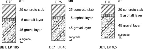
Using the adopted design approach (Eberhardsteiner et al., 2018; Spielhofer et al., 2013) the impact of the dynamic wheel loads due to longitudinal unevenness on the estimated service life of standard rigid pavement structures in Figure 4 (structure type BE1, load classes LK6.5, LK40 and LK185 according to the Austrian standard RVS 03.08.63 (FSV, 2016) and square slabs having plan dimension of $5\times 5$ $\left[\mathrm{m}\right]$) was assessed depending on the ${\mathrm{\Delta }}_{WLP}$-category and the chosen confidence level. The only difference between these pavement structures is the slab thickness (20, 25 and 29 $\left[\mathrm{c}\mathrm{m}\right]$).

Figure 4. Investigated rigid pavement structures.

The input variables of the unbound layers and the temperature gradients for the six climate periods are given in Tables 1 and 2. Thereby, typical values of the Young's modulus of concrete (30,000 $\left[\mathrm{M}\mathrm{P}\mathrm{a}\right]$) and asphalt (3500 $\left[\mathrm{M}\mathrm{P}\mathrm{a}\right]$) have been used. The assumed bending tensile strength of the concrete of 5.27 $\left[\mathrm{N}\cdot {\mathrm{m}\mathrm{m}}^{-2}\right]$ applies to concretes with natural aggregates and a confidence level of 95%. Standard dowels with a length of 500 $\left[\mathrm{m}\mathrm{m}\right]$, a diameter of 25 $\left[\mathrm{m}\mathrm{m}\right]$ and a corresponding dowel effectiveness number of 400,232 $\left[\mathrm{k}\mathrm{N}\cdot {\mathrm{m}}^{-1}\right]$ were considered. As described above the traffic load consists of representative distributions for the appearance of heavy goods vehicle (HGV) types, the gross vehicle weights and the static axles loads (characteristic traffic collective) and their dynamic wheel load increases caused by longitudinal unevenness (categorised by ${\mathrm{\Delta }}_{WLP}$).

Table 3. Reduction factors (RF) and limit values of the parameter ${\mathrm{\Delta }}_{WLP}$ at the five grades and various slab thicknesses.

	${\mathrm{\Delta }}_{WLP}$ for various slab thicknesses			Reduction factor
Grade	200 [mm]	250 [mm]	290 [mm]	RF [–]
G1	<6	<8	<16	>0.9
G2	<16	<21	<36	>0.7
G3	<26	<33	<46	>0.6
G4	<35	<45	<61	>0.5
G5	>35	>45	>61	<0.5

After computing the stresses due to traffic loads (static and dynamic) and those due to temperature loading with the Kirchoff's plate theory (Höller et al., 2019) and the enhanced Eisenmann's model (Houben, 2009), respectively, the $N_{ijk}$ for each axle i of each vehicle j and each climate period k has been estimated.

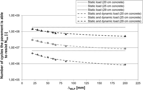
The following Figures 5 and 6 show the impact of the increased dynamic wheel loads due to increased longitudinal unevenness (expressed by the parameter ${\mathrm{\Delta }}_{WLP}$ of the weighted longitudinal profile) on the pavement damage (Figure 5) and on the theoretical service life (Figure 6). The difference between dotted and dashed lines describe the changes of the pavement damage and service life due to consideration of the dynamic wheel loads for the different slab thicknesses. The results for the nine categories of ${\mathrm{\Delta }}_{WLP}$ can be described by a power function. It is apparent that an increase of the longitudinal unevenness or higher ${\mathrm{\Delta }}_{WLP}$ causes more damage and reduction of the service life. As expected, thicker concrete slabs are more durable and less affected by the longitudinal unevenness. This trend was also confirmed by Rys (2019).

Figure 5. Impact of the variation of the longitudinal profile on the pavement damage for different pavement structures.

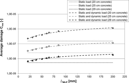
Figure 6. Impact of the variation of the longitudinal profile on the service life for different pavement structures.

4. Development of rating scheme for longitudinal unevenness

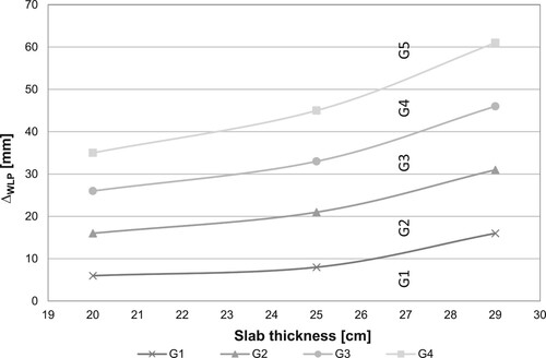
Since road unevenness can be subjected to a variation of layer thickness, it seems appropriate to consider the overall thickness of the existing concrete layer as a criterion for developing a rating scheme. Increased loads due to dynamic impulses (e. g. resulting from longitudinal unevenness) lead to increasing fatigue phenomena at the bottom of the concrete slab. Fatigue crack initiation starts at the bottom of the slab, which lead to a reduction of the effective thickness of the concrete layer resulting in a reduction of the residual life time. Hence, a connection to thickness reduction makes sense. Taking into account the correlation between the weighted longitudinal profile (${\mathrm{\Delta }}_{WLP}$) and the estimated service life of the above-mentioned pavement structures, a technically sound rating scheme has been developed (see Figure 8).

The following part of this paper moves on to describe the definition of a rating scheme for longitudinal unevenness for rigid pavement structure with slab thickness of 20 $\left[\mathrm{c}\mathrm{m}\right]$ (BE 1, load class LK 6.5). As defined in the Austrian specification RVS 08.17.02 (FSV, 2011) a newly constructed rigid road section is acceptable when the overall thickness of the concrete layer after the placement is not more than 2 $\left[\mathrm{c}\mathrm{m}\right]$ below the target layer thickness. This value was regarded as a threshold value and, hence results in a limiting thickness of 18 $\left[\mathrm{c}\mathrm{m}\right]$ for the investigated pavement structure (BE 1, load class LK 6.5) with a nominal concrete slab thickness of 20 $\left[\mathrm{c}\mathrm{m}\right]$. The decrease of the layer thickness from 20 to 18 $\left[\mathrm{c}\mathrm{m}\right]$ corresponds to a reduction of the technical service life from 6.5 to 3.3 million bearable standard load cycles (according to the design catalogue in RVS 03.08.63). Therefore, it defines a threshold in the evaluation scheme for longitudinal unevenness and refers to grade 5 (G5) according to the Austrian five-grade system.

As seen in Figure 7 the development of the technical service life with increasing longitudinal unevenness contains unrealistically high values of the parameter ${\mathrm{\Delta }}_{WLP}$. For this reason, the parameter was limited to 85 $\left[\mathrm{m}\mathrm{m}\right]$ and the correlation between the technical service life and ${\mathrm{\Delta }}_{WLP}$ was approximated by a second-degree polynomial function (see Figure 7). By applying this function, the threshold value of the parameter ${\mathrm{\Delta }}_{WLP}$ for grade G5 yields 35 $\left[\mathrm{m}\mathrm{m}\right]$. To determine the values of ${\mathrm{\Delta }}_{WLP}$ for the grades G1 to G4 the reduction of the layer thickness from 2 $\left[\mathrm{c}\mathrm{m}\right]$ is divided into four ranges with reduction of the slab thickness of 0.5 $\left[\mathrm{c}\mathrm{m}\right]$ for each range. Then the corresponding technical service life for each grade is determined. Appling the limit value of the service life for each grade in the function from Figure 7, the limit values of ${\mathrm{\Delta }}_{WLP}$ are subsequently calculated. Additionally, to the threshold value at grade G5, a warning value at grade G3 was introduced. The results are summarised in Table 3.

Figure 7. Determination of grades for the evaluation of the longitudinal profile of concrete slabs.

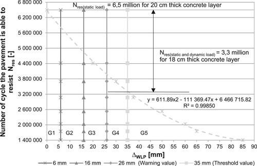
Figure 8. Correlation between reduction factor and parameter ${\mathrm{\Delta }}_{WLP}$.

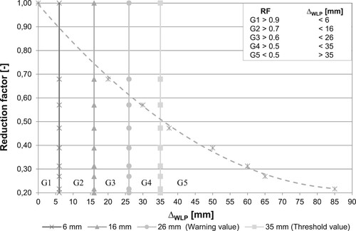
Table 4. Limiting values for ${\sigma }_{WLP}$ and ${\mathrm{\Delta }}_{WLP}$ according to Spielhofer and Ueckermann (2012) and corresponding reduction of the service life.

Limiting values	Target	Acceptance	Warranty	Warning	Threshold
Grade	1.50	2.50	2.87	3.50	4.50
${\sigma }_{WLP}$ [mm]	4	6	7	9	13
${\mathrm{\Delta }}_{WLP}$ [mm]	26	36	42	54	78
$N_{res,29\mathrm{c}\mathrm{m}}=185$ [Mill]	136	120	111	96	74
RF [–]	0.73	0.65	0.60	0.52	0.40

An easy way to calculate the reduction of the theoretical service life as a function of the longitudinal unevenness might be the use of a reduction factor (RF). As Figure 8 shows the RF is equal to 1 for perfectly even road sections. At grade G3 the reduction factor is 0.6 and ${\mathrm{\Delta }}_{WLP}$ 26 $\left[\mathrm{m}\mathrm{m}\right]$. Using this reduction factor RF and the number of load cycles the pavement is able to resist due to static loads $N_{res\left(staticload\right)}$, it is possible to estimate resulting service life due to static and dynamic loads $N_{res\left(staticanddynamicload\right)}$: (8) $N_{res\left(staticanddynamicload\right)}=N_{res\left(staticload\right)}\cdot RF$(8) The procedure described above for the definition of a rating scheme for longitudinal unevenness of rigid pavement structures with slab thickness of 20 $\left[\mathrm{m}\mathrm{m}\right]$ was applied also for pavement structures with slab thicknesses of 25 and 29 $\left[\mathrm{m}\mathrm{m}\right]$. From the data in Figure 9 and Table 3 it is apparent that there is a good correlation between the limit values for ${\mathrm{\Delta }}_{WLP}$ and the slab thickness for the five grades. Thus, knowing the slab thickness and the value of the parameter ${\mathrm{\Delta }}_{WLP}$ of an existing road section it is possible to rate it according to the presented evaluation scheme and assess the influence of the longitudinal unevenness on the service life.

Figure 9. Correlation between the parameter ${\mathrm{\Delta }}_{WLP}$ and the slab thickness for the defined five ${\mathrm{\Delta }}_{WLP}$-categories.

In a further step, using the derived correlation between $N_{res}$ and ${\mathrm{\Delta }}_{WLP}$, the resulting reduced service life $N_{res}$ for a concrete slab with a thickness of 29 $\left[\mathrm{c}\mathrm{m}\right]$ has been estimated for the limiting values from an earlier study (Spielhofer & Ueckermann, 2012) (see the first two rows in Table 4). The reduction factor at the threshold value is 0.4, which means 60% reduction of the initial design life of the considered pavement structure. Comparing the limiting values of the ${\mathrm{\Delta }}_{WLP}$ from Table 4 with those from Table 3 it is apparent that both are in the same range.

However, it should be noted that the definition of limiting values in Spielhofer and Ueckermann (2012) is based on an analysis of the physical effect of the unevenness on humans according to road categories for different speeds, travel times and waviness distributions by means of mathematical relations (Steinauer, 1992; Ueckermann & Steinauer, 2008). The current study presents a different perspective, it quantifies the impact of the increased wheel loads due to unevenness on the structural behaviour of different concrete pavement structures, therefore, the limiting values from both studies do not correspond entirely. Further, the derivation of general limiting values is a very complex problem, as the factors that should be accounted are not limited to the effects of traffic loading (e.g. climatic distresses like frost heave and thermal cracking). Two different road sections with different locations, layer thicknesses etc. assessed with the same value of the longitudinal indicator will experience different amount of deterioration and different rate of service life reduction.

5. Summary and conclusions

The results from this paper demonstrate the impact of the longitudinal unevenness assessed by the weighted longitudinal profile (WLP) on the performance of rigid pavements. This was possible on one hand by modelling characteristic vehicle types with their real static wheel loads using a modular approach. On the other hand, simulations of a ride were carried out using the developed axle assemblies and measured longitudinal profile data from the entire Austrian rigid highway network.

Consequently, the dynamic wheel loads for each axle assembly were calculated. The summarised results from the network-wide simulations are the distributions of the calculated dynamic wheel loads of the individual axle assemblies for nine ${\mathrm{\Delta }}_{WLP}$ categories.

The effect of the dynamically increased wheel loads on the damage and on the theoretical service life of rigid pavement structures typical for highways was demonstrated using an adopted version of the Austrian mechanistic-empirical design method for rigid pavements. A correlation between ${\mathrm{\Delta }}_{WLP}$, the slab thickness and the reduction of the technical service life was found.

Based on this correlation a technically sound rating scheme for longitudinal unevenness of rigid pavements has been derived. It allows the classification of the highway network into a five-grade system and the evaluation of the structural response of rigid pavements under dynamic wheel loads for the optimal utilisation of the service life of the pavement.

The following conclusions can be drawn from this paper:

• An increase of the longitudinal unevenness causes more damage and reduction of the service life.

• Thicker concrete slabs are more durable and less affected by longitudinal unevenness.

• A good correlation between ${\mathrm{\Delta }}_{WLP}$ and the dynamic wheel load is apparent, which demonstrates that WLP is a suitable assessment indicator for the distress due to dynamic wheel loads.

• The developed evaluation scheme allows for the assessment of the impact of the longitudinal unevenness on the service life for a known slab thickness and value of the parameter ${\mathrm{\Delta }}_{WLP}$ of an existing road section.

• Based on the introduced evaluation scheme, it was shown that the effect of dynamic loads can reduce the pavement life of up to 50%.

Disclosure statement

No potential conflict of interest was reported by the author(s).

Additional information

Funding

The authors gratefully acknowledge TU Wien Bibliothek for financial support through its Open Access Funding Programme and the Austrian Research Promotion Agency (FFG) through the project ‘LAST – Longitudinal unevenness-induced road damage due to dynamic wheel load variations’.

References

- Addis, R. (1992). Vehicle wheel loads and road pavement wear. Vehicle wheel loads and road pavement wear, Thomas Telford, London.
- ARA, Inc. (1993). Aashto guide for design of pavement structures.
- Bachmann, Ch., Gies, S., Wöhrmann, M., & Schrüllkamp, P. (2008). Realistische Lastannahmen für die Bemessung des Straßenoberbaus (Forschung Straßenbau und Straßenverkehrstechnik Vol. 998). Bundesministerium für Verkehr, Bau und Stadtentwicklung, Abteilung Straßenbau, Straßenverkehrs, Bonn.
- Bayraktarova, K., Eberhardsteiner, L., & Blab, R. (2017, June 28–30). Seasonal temperature distribution in rigid pavements. In A. Loizos, I. Al-Qadi, & T. Scarpas (Eds.), Proceedings of the 10th international conference on the bearing capacity of roads, railways and airfields (BCRRA 2017) (pp. 2087–2093). CRC Press.
- Bayraktarova, K., Eberhardsteiner, L., Zhou, D., & Blab, R. (2021). Characterisation of the climatic temperature variations in the design of rigid pavements. International Journal of Pavement Engineering, 23(9), 3222–3235. https://doi.org/10.1080/10298436.2021.1887486.
- Bilodeau, J., Gagnon, L., & Doré, G. (2017). Assessment of the relationship between the international roughness index and dynamic loading of heavy vehicles. International Journal of Pavement Engineering, 18(8), 693–701. https://doi.org/10.1080/10298436.2015.1121780
- Blab, R., Eberhardsteiner, L., Haselbauer, K., Marchart, B., & Hessmann, T. (2014). OBESTO - Implementierung des GVO- und LCCA-Ansatzes in die österreichische Bemessungsmethode für Straßenoberbauten, (Report), Vienna University of Technology, Institute of Transportation
- Buhari, R., Abdullah, M. E., & Rohnani, M. (2013). Dynamic load coefficient of tyre forces from truck axles. Applied Mechanics and Materials, 405(12), 1900–1911. https://doi.org/10.4028/www.scientific.net/AMM.405-408.1900
- Cebon, D. (1999). Handbook of vehicle–road interaction. CRC Press.
- Cole, D. J., & Cebon, D. (1989, June 18–22). Simulation and measurement of dynamic tyre forces. In 2nd International symposium on heavy vehicle weights and dimensions. CRC Press.
- Davis, L. E., & Bunker, J. (2011). Altering heavy vehicle air suspension dynamic forces by modifying air lines. International Journal of Heavy Vehicle Systems, 18(1), 1–17. https://doi.org/10.1504/IJHVS.2011.037957
- De Beer, M., & Fisher, C. (2013). Stress-in-motion (sim) system for capturing tri-axial tyre–road interaction in the contact patch. Measurement, 46(7), 2155–2173. https://doi.org/10.1016/j.measurement.2013.03.012
- Eberhardsteiner, L., Foltin, K., Bayraktarova, K., & Blab, R. (2018, April 16–18). Performance-related approach for rigid pavement design. In E. Masad, A. Bhasin, T. Scarpas, I. Menapace, & A. Kumar (Eds.), International conference on advances in materials and pavement performance prediction (AM3P 2018) (pp. 457–461). CRC Press.
- Eberhardsteiner, L., Foltin, K., Bayraktarova, K., Haselbauer, K., Pichler, B., Aminbaghai, M., Pratscher, P., & Blab, R. (2016). OBESTAS – Optimierte Bemessung starrer Aufbauten von Straßen, (Report), Vienna University of Technology, Institute of Transportation
- Eisenmann, J. (1975). Dynamic wheel load fluctuations – road stress. Strasse und Aubobahn, 26(4), 127–128.
- Eisenmann, J., & Leykauf, G. (2003). Concrete pavements – design and construction (in german). Ernst and Sohn.
- EN (2006). En 13036-5: Surface characteristics of road and airfield pavements – test methods – part 5: Determination of longitudinal unevennessindices.
- FGSV. (2012). Richtlinien für die Standardisierung des Oberbaus von Verkehrsflächen (RSTO), Cologne,Germany, Forschungsgesellschaft für Straßen- und Verkehrswesen (FGSV).
- Foltin, K., Eberhardsteiner, L., Bayraktarova, K., & Blab, R. (2016). Assessment of load transfer across transverse joints. 11th International conference on concrete pavements, San Antonio, Texas, 28.08 -01.09.2016.International Society for Concrete Pavements.
- FSV. (2011). RVS 08.17.02: Deckenherstellung, Vienna, Forschungsgesellschaft Straße-Schiene-Verkehr (FSV)
- FSV. (2016). RVS 03.08.63: Oberbaubemessung,Vienna,Forschungsgesellschaft Straße-Schiene-Verkehr (FSV)
- FSV. (2020). RVS 03.08.69: Rechnerische Dimensionierung von Betonstraßen, Vienna, Forschungsgesellschaft Straße-Schiene-Verkehr (FSV)
- Gagnon, L., Doré, G., & Richard, M. J. (2015a). An overview of various new road profile quality evaluation criteria: Part 1. International Journal of Pavement Engineering, 16(3), 224–238. https://doi.org/10.1080/10298436.2014.942814
- Gagnon, L., Doré, G., & Richard, M. J. (2015b). An overview of various new road profile quality evaluation criteria: Part 2. International Journal of Pavement Engineering, 16(9), 784–796. https://doi.org/10.1080/10298436.2014.960998
- Gajda, J., Burnos, P., & Sroka, R. (2018). Accuracy assessment of weigh-in-motion systems for vehicle's direct enforcement. IEEE Intelligent Transportation Systems Magazine, 10(1), 88–94. https://doi.org/10.1109/MITS.2017.2776111
- Gyenes, L., & Mitchell, C. (1992). The spatial repeatability of dynamic pavement loads caused by heavy goods vehicles. Third international symposium on heavy vehicle weights and dimensions, Queen's college Cambridge, UK, 28.06-2.07.1992.
- Harasim, P., & Gajewski, M. (2021). Research on the influence of pavement unevenness on heavy vehicles' axle loads variations with the use of tsd deflectometer. Roads and Bridges - Drogi i Mosty, 20(4), 425–439. https://doi.org/10.7409/rabdim.021.025
- Hassan, R. (2012). Highlighting dynamically loaded pavement sections with profile indices. Transportation Research Record: Journal of the Transportation Research Board, 2306(1), 65–72. https://doi.org/10.3141/2306-08
- Höller, R., Aminbaghai, M., Eberhardsteiner, L., Eberhardsteiner, J., Blab, R., Pichler, B., & Hellmich, C. (2019). Rigorous amendment of vlasov's theory for thin elastic plates on elastic winkler foundations, based on the principle of virtual power. European Journal of Mechanics – A/Solids, 73(0), 449–482. https://doi.org/10.1016/j.euromechsol.2018.07.013
- Houben, I. L. J. M. (2009). Structural design of pavements. http://www.citg.tudelft.nl/en/about-faculty/departments/structural-engineering/sections/pavement-engineering/education/lectures/
- Kamiya, K., Kawamura, A., Glattki, W., & Ueckermann, A. (2012). A routine monitoring method using weighted longitudinal profile. 7th Symposium on pavement surface characteristics: SURF 2012, Norfolk, Virginia.Virginia Tech Transportation Institute.
- Khavassefat, P. (2014). Vehicle–pavement interaction [Thesis (PhD), KTH Royal Institute of Technology].
- Khavassefat, P., Jelagin, D., & Birgisson, B. (2015). Dynamic response of flexible pavements at vehicle–road interaction. Road Materials and Pavement Design, 16(2), 256–276. https://doi.org/10.1080/14680629.2014.990402
- Khavassefat, P., Jelagin, D., & Birgisson, B. (2016). The non-stationary response of flexible pavements to moving loads. International Journal of Pavement Engineering, 17(5), 458–470. https://doi.org/10.1080/10298436.2014.993394
- Litzka, J., Molzer, C., & Blab, R. (1996). Modifikation der österreichschen Bemessungsmethode zur Dimensionierung des Straßenoberbaus (Schriftwnreihe Straßenforschung Vol. 465). Vienna: Bundesministerium für Verkehr, Innovation and Technologie.
- Machemehl, R., & Lee, C. E. (1974). Dynamic traffic loading of pavements. Center for Highway Research, University of Texas.
- Mitchell, C., Gyenes, L., & Philips, S. D. (1992). Dynamic pavement loads and tests of road-friendliness for heavy vehicle suspensions.. hird international symposium on heavy vehicle weights and dimensions, UK.Queen's college Cambridge.
- Mitschke, M. (1979). Verminderung der vertikalen Straßenbeanspruchung durch schwere Nutzfahrzeuge (Automobil-Industrie Vol. 24). Bundesanstalt für Straßenwesen (BASt).
- Mitschke, M., & Wallentowitz, H. (2004). Dynamik der Kraftfahrzeuge (4). Springer Berlin, Heidelberg.
- Múčka, P. (2013). Influence of road profile obstacles on road unevenness indicators. Road Materials and Pavement Design, 14(3), 689–702. https://doi.org/10.1080/14680629.2013.811823
- Múčka, P. (2015). Current approaches to quantify the longitudinal road roughness. International Journal of Pavement Engineering, 17(8), 659–679. https://doi.org/10.1080/10298436.2015.1011782
- Park, D., Papagiannakis, A., & Kim, I. T. (2014). Analysis of dynamic vehicle loads using vehicle pavement interaction model. KSCE Journal of Civil Engineering, 18(7), 2085–2092. https://doi.org/10.1007/s12205-014-0602-3
- Rossel-Khavassefat, P., Perret, J., Ould-Henia, M., & Delaby, M. (2022). An investigation on longitudinal unevenness indicators and their potential on surface characterisation. In Proceedings of the RILEM international symposium on bituminous materials (pp. 223–229). Springer International Publishing.
- Ruiz, M., Ramirez, L., Navarrina, F., Aymerich, M., & Lopez-Navarrete, D. (2019). A mathematical model to evaluate the impact of the maintenance strategy on the service life of flexible pavements. Mathematical Problems in Engineering, 1–10. https://doi.org/10.1155/2019/9480675
- Rys, D. (2019). Consideration of dynamic loads in the determination of axle load spectra for pavement design. Road Materials and Pavement Design, 22(6), 1–20. https://doi.org/10.1080/14680629.2019.1687006
- Rys, D., Judycki, J., & Jaskula, P. (2016). Determination of vehicles load equivalency factors for polish catalogue of typical flexible and semi-rigid pavement structures. Transportation Research Procedia, 14(0), 2382–2391. https://doi.org/10.1016/j.trpro.2016.05.272
- Spielhofer, R., Brozek, B., Maurer, P., Fruhmann, G., & Reinalter, W. (2009). Entwicklung eines Parameters zur Beurteilung der Längsebenheit (Schriftwnreihe Straßenforschung Vol. 582). Vienna: Bundesministerium für Verkehr, Innovation and Technologie.
- Spielhofer, R., Eberhadsteiner, L., Aichinger, C., Bayraktarova, K., Osichenko, D., Blab, R., Ueckermann, A., & Liu, P.. (2013). Längsunebenheitsbedingte Straßenschädigung durch dynamische Radlastschwankungen, (Report), Vienna, Austrian Institute of Technology and Vienna Unversity of Technology
- Spielhofer, R, Eberhadsteiner, L, Aichinger, C, Bayraktarova, K, Osichenko, D, Blab, R, Ueckermann, A, & Liu, P. (2013). Längsunebenheitsbedingte Straßenschädigung durch dynamische Radlastschwankungen.
- Spielhofer, R., & Ueckermann, A. (2012). Further investigations on the weighted longitudinal profile. 7th Symposium on pavement surface characteristics: SURF 2012, Norfolk, Virginia.Virginia Tech Transportation Institute.
- Steinauer, B. (1992). Vergleich stochastischer und periodischer Fahrbahnunebenheiten in Bezug auf Fahrkomfort. Bitumen, 54(1). Forschungsgesellschaft für Straßen- und Verkehrswesen (FGSV)
- Sun, L. (2001). Computer simulation and field measurement of dynamic pavement loading. Mathematics Computer in Simulation, 56(3), 297–313. https://doi.org/10.1016/S0378-4754(01)00297-X
- Sun, L. (2013). An overview of a unified theory of dynamics of vehicle–pavement interaction under moving and stochastic load. Journal of Modern Transportation, 21(3), 135–162. https://doi.org/10.1007/s40534-013-0017-8
- Sun, L. (2014). Optimum design of ‘road-friendly’ vehicle suspension systems subjected to rough pavement surfaces. Applied Mathematical Modelling, 26(5), 635–652. https://doi.org/10.1016/S0307-904X(01)00079-8
- Sweatman, P. (1983). A study of dynamic wheel forces in axle group suspensions of heavy vehicles. Australian Road Research Board.
- Ueckermann, A., & Oeser, M. (2015). Approaches for a 3d assessment of pavement evenness data based on 3d vehicle models. Journal of Traffic and Transportation Engineering (English Edition), 2(2), 68–80. https://doi.org/10.1016/j.jtte.2015.02.002
- Ueckermann, A., & Steinauer, B. (2008). The weighted longitudinal profile. A new method to evaluate the longitudinal evenness of roads. Road Materials and Pavement Design, 9(2), 135–157. https://doi.org/10.1080/14680629.2008.9690111
- Zahnmesser, W. (1981). Auswirkungen verschiedener Lastzugkombinationen auf die Strassenbeanspruchung (327). Bonn: Forschungsgesellschaft für Straßen- und Verkehrswesen (FGSV).