Runway groove closure prediction modelling by gene expression programming (GEP)

Abstract

Grooving on the runway is proven to improve frictional braking resistance and reduce the risk of hydroplaning during wet weather and maintain skid-resistant surfaces. Nonetheless, the runway grooves area deteriorates over time, and this groove closure is an outstanding distress that significantly diminishes grooves’ effectiveness. However, the degree of the deterioration of groove dimensions has not been quantified in a mathematical model yet. This paper is pioneering the predictive modelling by GeneXProTools 5.0 software for groove deterioration considering wheel pass number, load intensity, pavement layer thickness, and temperature as independent variables. The value of R2 achieved by the prediction model is 0.911, 0.921 and 0.924 for the training, validation and testing phase, respectively, which indicates that it fits with the experimental data very well. This model will render a meaningful contribution to airport authority in predicting grove deterioration and its serviceable length, leading to maintenance to reinstate the grooving.

KEYWORDS:

• Runway groove
• friction
• groove closure
• groove deterioration modelling
• GeneXProTools 5.0

Introduction

The friction of runway pavement is one of the vital factors regarding the safety of an aircraft's landing. Generally, skid resistance diminishes significantly during wet weather conditions, leading to the risk of aircraft moving off the runway (Pasindu, 2020). Over time research revealed that some special measures are needed to enhance the aircraft braking on the asphalt surface, especially in wet weather. Grooves render an exit of entrapped water from between aircraft tires and the pavement surface, which is quite similar to the car tire tread patterns. Thus, grooves improve frictional braking resistance and mitigate the risk of hydroplaning (White & Rodway, 2014). Since it allocates more flow depths for water to flow in the groove channel, it decreases the flow resistance and accelerates the water flow than the ordinary pavement surface (Pasindu, 2020).

Nonetheless, different factors need to be considered before grooving a runway, such as extreme hot or cold climates that are not suitable for grooving. Despite some limitations, runways are deploying grooving as the most common method utilised to develop aircraft braking performance, especially on the wet asphalt runways (White & Rodway, 2014). Federal Aviation Administration (FAA, 1997) developed a standard for runway grooving.

However, Runway grooves have some familiar distresses. Groove closure in the pavement surface at different airports is a common phenomenon and a severe form of distress. Groove closure certainly diminishes the grooves’ effectiveness, but the degree of the declination of groove dimensions has not been quantified theoretically (White, 2017). According to the general guidance of FAA's AC 150/5320-12C, airport operators should take immediate corrective measures to reinstate the groove if 40% of the grooves in the runway lost their dimension equal to or more than 50% from the original (FAA, 1997).

Groove closure depends on certain factors such as hot environments, aircraft speed, high wheel loads, and aircraft movements parallel to the grooves. There were some groove closure incidents in different international airports like Washington National airport, Brisbane Airport, Hong Kong airport, New Delhi International Airport, and Kualampur airport. The risk of groove closure is the primary concern why different airports are sensitive to runway grooving (White & Rodway, 2014).

White (2017) reviewed the management of skid resistance and friction on asphalt runway surfaces. Pasindu (2020) showed the impact of groove deterioration on runway frictional performance. An analytical approach was used to assess the frictional performance of pavements under wet conditions and variations caused by groove deterioration. Different groove depths were compared with the skid resistance performance of standard grooves, and their proximate performance was evaluated. This was achieved through simulated skid resistance variation with different groove depths. A simulation model was established using the finite element method. The finite element analysis computer software ADINA (2012) was employed to simulate the coupled tyre fluid pavement interaction (Pasindu, 2020).

Wang and Larkin (2019) expressed groove Life analysis on asphalt pavement. Groove deformation under aircraft loading was simulated using finite element models. The groove geometry data were scanned and collected at each grooving location using a high-performance laser system during the entire loading period. The simulations illustrated the stress distributions under similar aircraft wheel load (Wang & Larkin, 2019). However, Groove closure has yet to be quantified through mathematical modelling.

National Airport Pavement Test Facility (NAPTF) conducted a series of full-scale tests of airport pavement grooves on flexible pavements to assess pavement grooves’ operational performance. The groove geometry data was scanned using a high-performance laser system before and during the loading application under the examination (Wang & Larkin, 2019). Wang and Larkin (2019) discussed and evaluated the groove shape changes (Depth, width, and area) under a long term loading period between July 2014 and June 2016.

The study develops a predictive model of groove deterioration based on the NAPTF examination outcome by Wang and Larkin (2019). The modelling is conducted considering different independent variables such as wheel pass number, wheel load, sub-base thickness, asphalt thickness and maximum temperature, whereas groove cross-sectional area was the dependent variable.

GeneXproTools 5.0 was used to fabricate the GP model in this research. The software was utilised to stimulate a relationship between the groove closure with different input parameters such as wheel pass number, load intensity, pavement layer thickness, and temperature. The prediction equation evolved from the GEP model delivers valuable information to the airport runway pavement personnel for the prediction of groove closure derived from different input parameters and strengthen their Airport Pavement Management System (APMS).

Research objectives

Groove depth declination leads to loss of the runway's skid resistance performance and becomes a threat to the safety of the aircraft landing and movement on the runway. Therefore, it is significant to determine the degree of groove deterioration by conducting a prediction modelling since groove deterioration modelling has not been addressed and executed before. Hence, the research added a new dimension in the arena of predictive modelling of groove area declination. This modelling directs the authority to take steps before the specified groove closure occurs and thus ensures the runway is in safe operational condition.

The objective and the reasons for conducting the study are as follows:

1. Demonstrate the significance of runway grooving, including other means of improving runway friction.

2. Discuss different groove distress and the relevant factors in association with groove closure.

3. Develop a predictive model of groove deterioration. GeneXProTools 5.0 was employed to develop the GP model

The model helps predict the runway grooves’ operational performance and associated financial and maintenance programmes to the airport authority.

Grooving techniques in runways

Importance of grooving

Grooving is a technique of sawing and cutting in both the existing or new runway pavement to form the groove, which is proven a useful technique for rendering sufficient skid resistance and avoiding hydroplaning during rain (FAA, 1997).

The runway's wet situation is considered one of the significant factors for casing runway overruns and swings over accidents. Wet runway condition is a major contributing factor for runway overrun and swing over accidents during landings and take-off. Around 40% of accidents are related to landing overrun in Europe and account for nearly 2/3rd globally. As a result, runways necessitate being grooved worldwide to ensure satisfactory friction levels under all weather conditions (Pasindu, 2020).

Grooving system and requirements

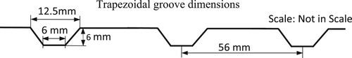
FAA developed a standard and groove configuration based on the tests and research conducted by Daiutolo (2012). The current FAA standard square groove dimensions are depth 6 mm (1/4 in), width 6 mm (1/4 in), and 38 mm (1 1/2 in.) centre to centre spacing, as depicted in Figure 1 (FAA, 1997).

Figure 1. FAA Standard groove design section (Adapted from FAA, 1997).

In addition to this, a minimum of 90% of the grooves should have a depth of at least 3/16 in. (5 mm), at least 60% of the grooves should have depth no less than 1/4 in. (6 mm), and 10% of the grooves may not exceed a depth of 5/16 in. (8 mm) as per FAA advisory circular AC-150/5370-10G (FAA, 2014). Hence, maintaining groove depth for adequate pavement friction during operation is critical (Pasindu, 2020). Nonetheless, groove depths can vary in construction and after construction due to deterioration in different ways (FAA, 2010).

Usually, grooves can be fabricated into the asphalt surface 4–8 weeks after the surface is constructed (White & Rodway, 2014). Grooves are generally fabricated across the runway surface, transversely to the runway length and perpendicular towards the runway's centerline (Wang & Larkin, 2019). Since the saw cutting techniques improved satisfactorily, a new trapezoidal-shaped groove was proposed by Patterson (2012) to evaluate with the standard rectangular groove (Pasindu, 2020). The trapezoidal groove dimensions consist of 1/2 in. (12.5 mm) at the top, 1/4 in. (6 mm) at the bottom, and distributed 2 1/4 in. (56 mm) centre to centre as shown in Figure 2 (Patterson, 2012). Newly designed trapezoidal grooves are practically constructed in the runways, as depicted in Figure 2 (Patterson, 2012).

Figure 2. Groove configurations of trapezoidal shapes (Adapted from Patterson, 2012).

Recently, FAA constructed rectangular and trapezoidal grooves in both rigid pavement and asphalt pavement at the National Airport Pavement Test Facility (NAPTF) areas to compare the performance of both grooves. The results demonstrated that the trapezoidal-shaped pavement groove design rendered some advantages over the current FAA standard square grooves that include better water evacuation, enhanced resistance to rubber contamination, integrity, and improved longevity (Fwa et al., 2014).

Considerations for grooving

According to the FAA advisory circular AC-150/5320-12C (FAA, 1997), runways serving or are expected to serve turbojets need to be grooved. Existing runways should be considered for grooving following some factors. Annual rainfall with accidental historical records related to hydroplaning at the airport should be checked. Furthermore, runway length quality of surface texture under dry or wet conditions such as polishing aggregate, insufficient macrotexture, improper seal coating, inadequate friction, and runway pavements strength must be taken into account. In addition to these, Transverse and longitudinal grades, any drop-offs at the runway ends due to terrain constraints, and crosswind effects should be considered. A reconnaissance survey should be conducted on the runway, including checking of bumps, bad or faulted joints, depressions, cracks, and the structural conditions specified in ACs 150/5320-6 and 150/5370-10 (FAA, 1997) before grooving (FAA, 1997).

Deterioration of runway fiction

Runway friction can deteriorate with time due to several factors such as mechanical wear and polishing action by aircraft tires during rolling or braking and contamination on the surface, mainly by rubber. These effects are related to the volume and type of aircraft traffic. Besides, variation in local weather conditions, pavement type (HMA or PCC), materials used in the original construction, and airport maintenance practices also influence runway pavement skid resistance (FAA, 1997).

Pavement structural failure, such as rutting, cracking, ravelling, joint failure, and settling, can trigger runway friction losses. Besides rubber deposition, other contaminants, such as oil spillage, dust particles, jet fuel, water, snow, ice, and slush, can prompt friction loss on runway pavement surfaces (FAA, 1997).

Methods used to improve runway friction

Runway grooving is a unique method that has now become popular to improve aircraft braking on wet asphalt-surfaced runways. Open Graded Friction Course is practical for surface water drainage improvement but becomes clogged by debris. On the contrary, Stone Mastic Asphalt is an open-graded mix that exhibits increased surface texture without the risk of clogging or closure. Prior to the grooving, coarse asphalt mixes consisting of 20 mm aggregates were utilised to attain better surface textures. Furthermore, Sprayed or ‘chip’ sealing renders significant surface texture and is commonly adopted in regional and remote airports (White, 2017; White & Rodway, 2014).

Runway friction determination

Advisory Circular AC 150/5320-12D renders the necessary instructions and guidelines for maintaining skid-resistant airport pavement surfaces and the evaluation process of surveys of runway friction for pavement maintenance (FAA, 2016).

Friction survey frequency and requirements

When any runway end operates wide-body aircraft (such as B-747, DC- 10, MD-11) 20 per cent or more of the total aircraft, the authority should select the next higher level of aircraft operations to decide the minimum survey frequency in Table 1. This Friction Survey considers the average mix of turbojet aircraft that can be operated on any particular runway as guidance for the initial scheduling of runway friction surveys. Moreover, the friction survey schedule is sufficient to identify and predict marginal friction conditions in time to initiate corrective measures (FAA, 2016).

Table 1. Friction Survey Frequency (Adapted from FAA, 2016).

Turbojet Aircraft Landing per Runway End (Nos./day)	< 15	16–30	31–90	91–150	151–210	> 210
Minimum Friction Survey Frequency (Time)	One Year	Six Months	Three Months	One Month	Two Weeks	One Week

Friction level classification

The runway friction is represented by the Greek letter µ (Mu). Table 2 delineates the friction values to categorise the friction level operated at a different speed. The speed of the Vehicle comprises the approved Continuous Friction Measuring Equipment (CFME) for executing the friction survey utilises either 40 mph (65 km/h) or 60 mph (95 km/h). A complete survey should incorporate both speeds since it indicates the condition of the surface’s overall micro and macrotexture (FAA, 2016).

Table 2. Friction level Classification for Runways (Adapted from FAA, 2016).

	Average Friction Value (µ)
Vehicle Speed	Minimum	Maintenance planning required	Friction Tester
40 mph (65 km/h)	0.50	0.60	Airport Surface Friction Tester
	0.50	0.60	Dynatest Runway Friction Tester
	0.43	0.53	Griptester Friction Meter
	0.42	0.52	µ Meter
60 mph (95 km/h)	0.34	0.47	Airport Surface Friction Tester
	0.41	0.54	Dynatest Runway Friction Tester
	0.24	0.36	Griptester Friction Meter
	0.26	0.38	µ Meter

The CFME operator records the data of 500 feet (150 m) and 1,000 feet (300 km) from the threshold end during conducting friction surveys on runways at 40 mph (65 km/h) and 60 mph (95 km/h), respectively. When the average µ value evolves from the wet runway surface is more than the Minimum Friction Level but fewer than Maintenance Planning Friction Level as indicated in Table 2, no corrective measure is required for that surveyed section. However, when the averaged µ value of the wet pavement surface falls lower than the Minimum Friction Level as per Table 2, corrective measures should be engaged immediately and the reason’s determination. Besides, a NOTAM (Notice to Air Missions) mentioning ‘Slippery when wet' is issued to demonstrate the runways’ state (FAA, 2016).

When friction values attained from the survey fulfil the criteria depicted in Table 2, no texture depth measurements are required. However, when the friction values do not satisfy the requirements, the airport authority must conduct the texture depth investigation. The threshold of Estimated Texture Depth (ETD) and the time of action are demonstrated in Table 3. When the average ETD index of one-third of the runway length is less than 0.76 mm but more than 0.40 mm, the airport authority should launch an initiative to rectify the texture deficiency within a year. Nonetheless, rehabilitation actions are urgent when ETD threshold values are equal to or exceed the level of the critical condition. The texture depth examination should always be done in non-grooved areas, such as the vicinity of transverse joints, but as close to heavily trafficked areas in a grooved pavement (FAA, 2016).

Table 3. Threshold Values of ETD and the time of action, Adapted from (FAA, 2016; Di Mascio & Moretti, 2019).

Runway groove distress

Grooves initiate different potential distress mechanisms that are not found in an ungrooved pavement surface. Some common distresses related to grooving are rubber contamination, groove depth lessening due to surface erosion, edge break, and groove closure (White & Rodway, 2014).

Rubber deposition can occur in touchdown zones on both grooved and ungrooved runways. NASA revealed that transversely grooved runway pavements generate fewer rubber deposits during aircraft touchdown actions than non-grooved pavements. Nonetheless, grooved pavements need to remove rubber contamination frequently to maintain groove effectiveness.

Groove depth can be reduced due to the erosion of the fine particles from between the larger aggregates. However, this dislocation of fines can enhance the general texture of the surface, which somehow counters the reduction in the grooves’ effectiveness. Erosion of Asphalt surface is preliminary created by jet blast. Besides, aged binder expedites the disposition of fine aggregate particles and binder from the surface. The rate of erosion can be amplified due to some reasons such as using unsound aggregates in asphalt production, using binder prone to rapid aging, inappropriate aggregate gradation in the manufacture of the asphalt, and unfavourable environmental conditions (White & Rodway, 2014).

Edge breaking in the groove occurred due to the bitumen binder's cohesive failures rather than adhesive failures of the aggregate-binder interface in the hot mixed asphalt (HMA). As a result, a more temperature resistant binder is searched to secure cohesion and stiffness of pavement at high temperatures. Conversely, this will diminish the aggregate loss associated with edge breaking and finally prevent groove closure (White & Rodway, 2014).

Some other distresses, such as spalling, cracking, wearing, and erosion, are inherent to HMA pavements and can be found in grooved and ungrooved asphalt surfaces. In addition to these, migration in asphalt resultant from the flow may turn to a wavy groove shape. Most groove collapse attributed to grove closure occurred due to plastic flow and was closely connected to the characteristics of asphalt containing binder and aggregates (Apeagyei et al., 2007).

Groove failure mechanisms

One of the mechanisms involved with groove failure is plastic flow resulting from the viscous flow, which is quite similar to the rutting mechanism in ungrooved asphalt surfaces. Microscopic analysis of asphalt suggested that cohesive (or stiffness) deficiency is more prominent than adhesive failure. Finally, groove closure should be connected to binder characteristics, which are the function of temperature, loading time, and aging (Emery, 2005a; 2005b). Another form of groove failure is edge breakage due to the horizontal stresses induced by aircraft tires. Moreover, repeated application of this stress level leads to edge failure on the unsupported groove edges. The investigation suggested that this edge beak is a cohesive failure and depends on the binder's viscosity (stiffness). Nonetheless, asphalt becomes more brittle, and this groove edge breakage mechanism could be more critical in cold weather conditions than hot environments. Furthermore, age-induced hardening, freeze–thaw cycling, moisture effects, and chemicals’ de-icing could enlarge the edge breakage (Apeagyei et al., 2007).

Groove closure

Groove closure is the prominent form of groove distress, which indeed reduces its effectiveness. However, the degree of groove area declination has not been quantified in a theoretical process. Friction testing is useful to measure the effect of partial groove closure (White & Rodway, 2014). According to FAA’s AC 150/5320-12C, if 40% of the grooves in the runway lost its shape equal to or less than 3 mm in depth and/or width in a successive length of 457 m, the effectiveness of grooves for preventing hydroplaning has been declined significantly. As a result, the airport authority should reinstate the groove shape immediately (FAA, 1997).

Groove closures are a common phenomenon in hot environments. It is observed in summer due to consecutive high pavement temperatures, especially in the asphalts made with relatively soft binders. It can also happen in the locations where aircraft travel slowly and parallel movement to the grooves, such as runway entry and exits. Furthermore, relatively new asphalt surfaces are more susceptible to groove closure besides high wheel loads. Re-sawing of closed grooves may create foreign object debris (FOD) hazards due to breaking off poorly supported asphalt. This issue can be solved by laying a new asphalt overlay around 60 mm and grooving it once curing (White & Rodway, 2014).

Groove closure in a different airport

Runways in hot environments are indifferent to grooving because of the possibility of groove closure. For instance, the major concern was that grooves in a runway in Dubai airport were closed due to hot weathering conditions. Therefore, to improve the friction and surface texture, a layer of 25 mm sized surface mix was deployed that was examined by using a Griptester (White & Rodway, 2014).

Recently, during the hot weather period, Brisbane airport's newly overlaid runway had groove closure at both ends. However, it was not anticipated since the previous overlay with the same multi-grade binder existed without groove closures for 12 years. Hong Kong airport also observed similar groove closure issues immediately after the construction and opening for the traffic. Nonetheless, the asphalt surface was laid about a year before the inauguration (White & Rodway, 2014).

At New Delhi International Airport, test grooves were sawn at the shoulder consisting of asphalt with unmodified 60–70 penetration bitumen, and the groove edges were ragged, and displacement of aggregates occurred. Consequently, the authority decided not to groove the main runway until several years of its operation (White & Rodway, 2014).

There are some factors to be considered when deciding to groove to a runway. Minimum curing times after asphalt laying and groove installation are four weeks. However, At Washington National airport, grooving was completed just a week after the laying of asphalt. Consequently, grooves were closed under the aircraft traffic, and rejuvenation became essential. Although the Australian regional runway was grooved for a shorter period of 10 days after placing the asphalt, the grooves, fortunately, remained steady during operation (White & Rodway, 2014).

Maintenance techniques for high skid resistance runways

Different techniques are available for removing rubber deposits, including other contaminants from runway surfaces. Some well-known methods are high-pressure water, chemical cleaning, and mechanical grinding. After removing contaminant and heavy-duty cleaning, the authority should remeasure the friction (µ) values by CFME and ensure that it returns within the 10 per cent frictional state of the adjacent surfaces. The contaminant removal practices are discussed below:

High-pressure water cleaning

The contaminants are blasted from the pavement surface to the edge of the runway by employing a series of high-pressure water jets. The technique is economical and eliminates the rubbish from the pavement surface with minimal interruption to the operators. Moreover, this high-pressure water blasting can be utilised to develop smooth pavements’ surface texture. However, the water pressure may vary from equipment to equipment and have the potential to damage the pavement.

Chemicals washing

Chemicals used on runways should meet the federal, state, and local environmental legislative requirements. Chemical solvents with a base of cresylic acid and a blend of benzene are found useful to remove contaminants on both PCC and HMA runways. Generally, alkaline chemicals are utilised to remove rubber deposits on the HMA runways. Detergents made of metasilicate and resin soap are efficient on PCC runway surfaces to remove oil and grease. However, It is also imperative to dilute the chemical solvent to diminish the effect of the surrounding environment, including vegetation, wildlife habitats or drainage systems (FAA, 2016).

Mechanical removal

Mechanical grinding techniques utilise the corrugating method to successfully remove heavy rubber deposits from HMA runway pavements and enhance surface friction characteristics significantly. A thin milling operation is executed up to a depth of 4.8 mm on pavement surfaces contaminated with rubber buildup, bleeding or worn that improves the surface friction coefficient to a greater extent (FAA, 2016).

Groove life analysis at the FAA national airport pavement test facility (NAPTF) centre

Federal Aviation Administration (FAA) developed a standard specification of airport groove Configuration during the construction of runway or in-service condition. National Airport Pavement Test Facility (NAPTF) made a series of full-scale tests of airport pavement grooves on both flexible and rigid pavements in recent years to assess pavement grooves’ construction quality and operational performance. Besides, the FAA launched a computer programme, namely ProGroove, to identify and analyse grooves. The groove geometry data was scanned using a high-performance laser system before and during the loading application under the examination. Rectangular grooves in asphalt pavements were installed, and deformations under aircraft loading were evaluated that unveiled the asphalt pavement groove life and effect of aircraft traffic loading effect (Wang & Larkin, 2019).

Groove installation

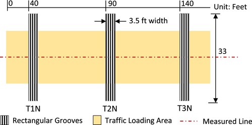
Recently, FAA constructed rectangular grooves in asphalt pavement at the National Airport Pavement Test Facility (NAPTF) areas to asphalt pavement groove life and effect of aircraft traffic loading effect. Three grooved sections areas were considered, including different pavement structures and denoted as T1N, T2N, and T3N contains 27 rectangular grooves in each section having a width of 3.5 ft as demonstrated in Figure 3 (Wang & Larkin, 2019).

Figure 3. Layout of groove areas and measured line (Adapted from Wang & Larkin, 2019).

Pavement structural conditions and associated loading

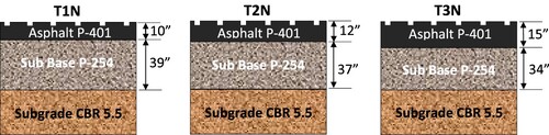
The formation was constructed over a clay subgrade material with a design CBR of 5.5, a variable thickness layer of P-154 granular subbase, and an inconstant thickness surfacing layer of P-401 asphalt, as illustrated in Figure 4.

Figure 4. Profile of structural set at different test sections.

The full-scale test started on 09/15/2014 using the National Airport Pavement Test Vehicle (NAPTV), which consists of a six-wheel triple tandem with a loading capacity of 55 kips per wheel at a speed of 2.5 mph. Afterwards, the wheel load was escalated to 65 kips after the completion of 30,030 wheel passes. The real scale aircraft loading tests were conducted on asphalt pavement at NAPTF on the Construction Cycle 7(CC7) from July 2014 to June 2016. A total number of 37290 vehicle passes were provided on the asphalt surface consisting of rectangular groove sections (Wang & Larkin, 2019).

Groove area corresponding to the loading

The data were gathered using an automatic device containing a 3D high-resolution portable profiler with a laser sensor installed on a portable truss profiler during testing. The profiler observed the groove shape changes and detected the displacement based on a criteria line. Wang and Larkin (2019) discussed and evaluated the groove shape changes under the long term loading period.

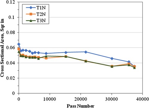
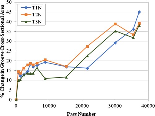
The investigation determined the depth, width, and cross-sectional area of the grooves between the loading period of July 2014 to June 2016, and the vehicle pass number was 37290, as demonstrated in Figure 5 (Wang & Larkin, 2019).

Figure 5. Groove Cross-Sectional Area With respect to Pass Number (Wang & Larkin, 2019).

The per cent (%) change in Groove Cross-Sectional Area with respect to Wheel Pass Number is portrayed in Figure 6. The Figure delineates that the grooves cross-sectional area was reduced up to 40-45% after execution of 37290 number wheel passes. These grooves exhibit serviceable conditions until they reach 50% or more per cent change in their original cross-sectional area.

Figure 6. Per cent (%) change in Groove Cross-Sectional Area to wheel Pass Number.

Predictive modelling by gene expression programming (GEP)

Gene expression programming (GEP)

Ferreira (2001) invented a robust technique that can able to solve critical mathematical and statistical problems named Gene expression programming (GEP), which follows the genotype system. Gene expression programming (GEP) is similar to genetic algorithms (GAs) and genetic programming (GP), which customs populations of individuals utilising genetic algorithms and selects them according to fitness and presents genetic disparity using one or more genetic operators (Ferreira, 2001). Hence, it is a hybrid derived from the evolutionary algorithms of genetic algorithms (GA) and genetic programming (GP) (Tarawneh, 2018).

Each programme (chromosome) is acted effectively, and its fitness is accomplished through the fitness function. The fitness indicates how well the chromosome is competitively fit with the rest of the population. Chromosomes are then undergoing further development according to their fitness. Typically, when the fitness level is higher, there is more chance of reselected than chromosomes with less fitness. The selected programmes are then experiencing more advanced developments with genetic changes, including mutation, recombination, and others. As a result, new descendants of chromosomes having different characteristics are created through the same developmental process. This procedure is continued until the pre-determined stopping criteria are attained (Tarawneh, 2018).

The GP's fundamental genetic operators are akin to GA, for instance, mutation, reproduction, and crossover, except for the expression tree or syntax tree that expressed the GP rather than conventional codes. Moreover, It can be articulated in linear mathematical formulae. Generally, the leading operators in GP are Mutation and Crossover, and the initial population is randomly developed through individual computer programmes. The selection process of individuals depends on their fitness for crossover (Leong et al., 2018). However, in GEP, evolution happens typically during each iteration subjected to the genetic variation that occurred by mutation, recombination and other genetic operators. In GEP, the mutation is the most significant genetic operator that involves changing any component of the gene's head or tail and replaced with another selected element from the function or terminal set, thus changing the genomes (Tarawneh, 2018). Mutations can take place anywhere on the chromosome. However, in the heads, any symbol or function can replace with another function or terminal. On the contrary, in the tails, terminals can only transform into terminals (Ferreira, 2001).

Recombination is the method where two chromosomes are paired and crossed over and split at some point to switch their components and emerge into new individuals (Tarawneh, 2018). In the GEP Transposition process, an insertion sequence is introduced somewhere between chromosomes within a chromosome or even within a single gene. In Transposition, it must preserve chromosome length and gene structure, and it makes a shift at the insertion point, and simultaneously deletion occurs at the end of the head. In the Inversion system, a small sequence with two elements in any gene domain is chosen randomly within a chromosome then inversion appears (Ferreira, 2001).

In GEP, every gene possesses a fixed length and constitutes a head that includes functions (e.g. +, –) and terminals (representing the input variables), and a tail comprises terminals only (Tarawneh, 2018).

The terminals are represented as the input variables (i.e. x and denoted by d0, and d1) and numerical constants (symbolised by c0, c1, and so on) in the expression tree (ET). On the other hand, the functions are designated as the internal nodes, for instance, different arithmetic operations (i.e. +, −, *, /, Sqrt), certain mathematical operations (i.e. ln, sin, cos, exp), along with various conditional operations like if, greater, equal, then, and else. This arrangement of terminals and functions is determined as a primitive set in GEP (Leong et al., 2018).

Modelling procedure

GeneXproTools is a powerful software package that can be utilised to conduct a symbolic regression analysis founded on Gene Expression Programming (GEP) (Ferreira, 2001, 2006). The software package lucidly renders modelling solutions and illustrates the combined model's mathematical equation to the users. Moreover, GenXProTools is a simple to run consisting efficient tool within the GEP technique, which combines the inherent merits of Genetic Programming and Genetic Algorithms (Fernando et al.,  2009).

Leong et al. (2018) predicted the compressive strength of soil-fly ash geo polymer derived from the different mix designs comprised of a percentage of fly ash, soil, hydroxide, alkali activator/ash, ratio of silicate/hydroxide, and water as essential input variables to the output using GEP technique.

Hajihassani et al. (2019) obtained a gene expression programming (GEP) model algorithm to estimate the convergence of tunnels consisting of six input parameters, namely, tunnel depth, cohesion, frictional angle, unit weight, Poisson’s ratio, and elasticity modulus, while the cumulative convergence was utilised as the model’s output.

Pham et al. (2021) developed a reliable model using the GEP technique for predicting the unconfined compressive strength (UCS) of soil stabilisation by cement and fly ash. The variable includes the plastic limit, the liquid limit, the percentage of clay, the percentage of silt, the percentage of sand, the percentage of organic in the soil, the total water content, the curing period, the cement content, the fly ash content, the CaO content in fly ash, the CaO/SiO2 ratio in fly ash, and the loss of ignition of fly ash, respectively.

In this paper, GeneXProTools 5.0 was implemented to develop the GEP model in this research. The software was utilised to generate a relationship between the groove areas changing with different input parameters.

In general, the task of linking input parameters is followed by various functions in GEP. Four basic operators (+, −, ×, /) and some more functions, including x², √3, ln, and exp, were used in this modelling. A GP-based model is assembled by expression trees (ETs), by which mathematical equations are derived from these ETs. Usually, an ET consists of several genes termed sub-ETs, each of which possesses some nodes. Each node may contain either any of the input parameters or a function. Some constants are evolved to adjust the equations in the model.

The numbers of chromosomes and sub-ETs as genes are two significant parameters that play a vital role in the accuracy of a model. However, a limited number of chromosomes and genes could lead to inferior accuracy and generate a complex and inefficient equation. As a result, there should be an optimum number of these crucial parameters for any specific model. Head size is another important parameter determining the complexity or maximum size of each sub-ET branch in the model. Different provisions of functions and original & derived variables and constants are evolved in the terminals in order to model the data (Gepsoft, 2020). The maximum number of chromosomes and head sizes may not be utilised in a model. A linking function is essential to link the sub-ETs in the model when the number of genes is more than one. The addition is used as a liking function among different mathematical operators to link the sub-ETs.

The datasets from the experiments should be divided into training, validation and testing parts. Modelling was continued until the coefficient of determination (R²) became higher for all training and validating phases (Gepsoft, 2020). GEP model development begins with the determination of the optimum modelling parameters.

In practice, there is no standard way to identify the optimum number of sub-ETs or chromosomes. However, the acceptable technique is to use one or more sub-ETs along with some chromosomes and heads and run the model. Afterwards, monitor the results and adjust the parameters such as the number of chromosomes, Genes (sub-ETs), heads, functions, linking function and several genetic operators until attaining optimum accuracy. The optimal parameters were established consecutively by conducting many trials using the GeneXproTools 5.0 software (Tarawneh, 2018).

One can evaluate and visualise the actual design process by surveying the real-time monitoring of different model fitting charts and statistics shown in the Run Panel. The features include different curve fitting charts, the residuals plot, the scatter plot, the correlation coefficient, the R-square, and the fitness. The correlation coefficient and R-square indicates the correlation between the model output and the target set by the actual values of the dependent variables (Gepsoft, 2020). It is significant to have a model trained and validated with approximately the same accuracy (Leong et al., 2018).

Data management and model configuration

Data collection and input variables

The wheel load and pass number, Sub Base, and asphalt thickness data were extracted from asphalt pavement groove life and effect of aircraft traffic loading investigated by Wang and Larkin (2019) at FAA National Airport Pavement Test Facility (NAPTF). The maximum recorded temperature during the loading period was collected from the website ‘timeanddate.com’ (2020).

The input variables and response variables are inputted as X and Y. In this GP model, the inputs are Wheel pass number (d0), load (d1), Subbase Thickness (d2), Asphalt Thickness (d3), and Maximum temperature (d4), respectively and the response variable and output parameter is Groove Cross-Sectional Area (Y).

General importance of the input variables

The input variables are Wheel pass number (n), Wheel load (L), Subbase Thickness (TSB), Asphalt Thickness (T_a), and Maximum temperature (t_max) correspondingly.

Landing gear configuration and gross aircraft weight dominate airfield pavement design and reveal structural fatigue in Cumulative Damage Factor (CDF), which is the ratio of applied load repetitions to allowable load repetitions. Among other aircraft, B - 777 - 300 ER has the highest CDF for flexible and rigid pavements. Emery (2005a, 2005b) examined the deterioration of grooves of asphalt on Australian runways. Wheel loads in association with slow movement and heavy aircraft were accountable for most groove closure in Australia (Emery, 2005a, 2005b).

Variability in pavement layer thickness makes the variations in pavement performance significantly. Subgrade stiffness, granular subbase thickness, and asphalt thickness are the variable parameters that influence the variability of predicted deformation performance (Valle & Thom, 2020).

In general, asphalt rheological properties are governed by temperature (Apeagyei et al., 2007). Hence, groove closures have occurred more severely in hot environments (White & Rodway, 2014). Furthermore, groove wear and closure are significantly related to the plastic flow of the HMA. Aircraft loading in higher temperatures renders plastic flow and displaced aggregates along the wheel tracks (Apeagyei et al., 2007). Asphalt pavements that are subjected to temperature fluctuations daily or seasonally are more susceptible to fatigue damage rather than at a specific temperature (Safaei & Hintz, 2014).

Since the input variables could significantly affect the output, the correlations between the input variables and the output results could be significant for determining the groove area. Moreover, variables with substantial value lead to the positive consequence of the output and vice versa. Nonetheless, insignificant variables might diminish the accuracy and overall performance of the model.

Data set selection

The data were partitioned into training and validation divided randomly, shuffled, odd and even to avoid overfitting and create a robust model. The training dataset is employed to construct and standardise the model applying modelling strategy to predict a correlation between dependent and independent variables.

The validation dataset needs to check and selected the models during the design process. Usually, in machine learning, a validation set is used to tune the model hyperparameters. The testing dataset is a sub-set of the validation set reserved to test and evaluate the accuracy and generalisation performance of the final model. This test set cannot be used until the training has been completed and the optimal model structure and parameters have been established (Gepsoft, 2020).

In this research, 67%-80% of the samples were considered as the training data set, and 20%-33% were regarded as the validation data set by partition, random shuffle, odd, and even sampling from the entire dataset. Moreover, the validation datasets are split up by odds, even, top half, bottom half, and shuffled sampling categories. However, the testing set is not employed during the training stage but is utilised to test the generalisation ability of the generated model. In this way, several models will be fabricated accordingly. Afterwards, those models that had better coefficients of determination (R² greater than 0.9) were selected for further evaluation against each other to determine the best model to estimate the predicted groove cross-sectional areas. Moreover, the statistical evaluation of inevitable errors appeared in the training and validation phases, including root mean square error (RMSE), mean absolute error (MAE), relative absolute error (RAE), and root relative squared error (RRSP) were compared. Generally, the errors are lower when the model achieves a higher fitness level (Shahmansouri et al., 2020).

Model configuration

In order to generate the combined model in GenXProTools:5, the following settings were employed, as depicted in Table 4.

Table 4. GEP Model configuration.

General input Settings
Variables:
Independent variables input:
• Wheel Pass number (Number):	d(0)
• load (Kips):	d(1)
• Subbase Thickness (inch):	d(2)
• Asphalt Thickness (inch):	d(3)
• Maximum temperature (°C):	d(4)
Dependent variable input:
• Groove Cross-Sectional Area (Sq-inch)	Y
Output: GEP model estimate (Sq-inch)
General Settings:
Number of training samples:	54–64
Validation samples:	9–13
Testing samples:	8–13
Number of chromosomes:	30–60
Head size:	8–14
No of Gene:	3–5
Fitness Function:	RMSE
Linking Function:	Addition
Stopping criterion:	Maximum Fitness
Numerical Constants
Constants per gene	10
Lower bound	−10
Upper bound	10
Data Type	Floating-point
Genetic Operators
Mutation	0.00138
Inversion	0.00546
Gene Recombination	0.00277
Gene Transposition	0.00277

The dataset (a total number of 81) was divided into training (54-64 Nos.), validation (9-13 Nos.), and Testing (8-13 nos.) sets to assemble the GEP models. The addition was selected as the linking function, whereas the Root Mean Squared Error (RMSE) was used as the fitness function. A total number of 30–60 chromosomes, 8–14 head sizes, and 3–5 genes were employed in the GEP models. Different fundamental genetic operators were selected, including mutation, inversion, Gene recombination and Gene transposition accounting for 0.00138, 0.00546, 0.00277 and 0.00277 consecutively.

GeneXproTools got numerous built-in mathematical functions (such as +, −, ×, /, x2, √3, ln, and exp) that allows users to develop custom functions to advance models with them. This extensive range of mathematical functions permits to fabrication of highly sophisticated and more precise models. The GEP models utilised seventeen functions as delineated in Table 5. Arity is the number of arguments used by the functions in the function set. The number of arguments it can be permitted to take is a minimum of 1 and a maximum of 4 by deciding the arity. However, the value of arity is chosen 1 and 2 for different symbolic functions during model configuration. By default, the weight of each function is considered 1. However, the probability of a function being included in the models can be augmented by increasing its weight, and a maximum weight of 6 was allocated for some functions.

Table 5. Symbolic Function Settings used in GEP Model.

Symbolic Function Set
Function	Symbol	Weight	Arity
Addition	+	6	2
Subtraction	–	6	2
Multiplication	*	6	2
Division	/	3	2
Exponential	Exp	3	1
Natural logarithm	Ln	3	1
x to the power of 2	X^2	3	1
x to the power of 3	X^3	3	1
Square root	Sqrt	3	1
Cube root	3Rt	3	1
Arctangent	Atan	3	1
Minimum of 2 inputs	Min2	3	2
Maximum of 2 inputs	Max2	3	2
Average of 2 inputs	Avg2	6	2
Hyperbolic tangent	Tanh	3	1
Complement	NOT	3	1
Inverse	Inv	3	1

Results and discussions

The strength of the generated model in predicting the targeted output is assessed by evaluating some statistical indicators such as coefficient of determination (R²), RMSE, MAE, RAE, and RRSP for the training and validation and testing datasets. R² is a representation utilised to evaluate how perfectly the model describes and execute the prediction values. RMSE indicates how spreads out (standard deviation) the residuals from the regression line. MAE estimates how far or prediction differs from actual values. RAE also measure predictive models performance by estimating the ratio of comparing a mean error (residual) to errors generated by the insignificant model. RMSE is a standard way to estimate the error of a prediction. RMSE can be obtained by dividing the vector of predicted values by the vector of experimental values. The MAE, RMSE, RAE and RRSE values can be obtained by using the following interpretations (Nazari et al., 2015): (1) $\begin{array}{rl}\text{RMSE}& =\sqrt{\frac{1}{n}\sum _i{(t_i-o_i)}^2}\end{array}$(1) (2) $\begin{array}{rl}\text{MAE}& =\frac{1}{n}\sum _i|t_i-o_i|\end{array}$(2) (3) $\begin{array}{rl}\text{RAE}& =\frac{\sum _i|t_i-o_i|}{\sum _i\left|t_i-\frac{1}{n}\sum _i{t}_i\right|}\end{array}$(3) (4) $\begin{array}{rl}\text{RRSE}& =\sqrt{\frac{\sum _i{(t_i-o_i)}^2}{\sum _i{\left(t_i-\frac{1}{n}\sum _i{t_i}_i\right)}^2}}\end{array}$(4) where t_i indicates the target parameter, o_i is the output parameter and n represents the number of datasets.

Comparison of selected GEP models

Three models have been selected, as depicted in Table 6, from the developed models enlisted in Appendix I, which attained an R² value greater than 0.9. R² values above 0.90 signify the proximity of the predicted results to the experimental values with improved accuracy and indicate the function's fitness level defined controlling the dataset well. A higher value of R² in the training phase delineates an excellent consistency of the final function. However, a significant difference of R² between the training and validation phase surge the deviation in the model and escalate errors.

Table 6. Selective Models with Parameters and Results including Fitness and Errors.

							Errors
GEP Model No.	Dataset Partitioning (Training & Validation)	Phase	Sample Size (Nos.) & Sampling		Fitness	R^2	RAE	RMSE	MAE	RRSE
GEP 5	Partition	Training	62	All	998.50	0.935	0.2602	0.0015	0.0011	0.2677
		Validation	10	Odd	997.13	0.958	0.5394	0.0029	0.0026	0.5232
		Testing	9	Even		0.962	0.6419	0.0029	0.0027	0.6149
						Σ/3	0.4805	0.0024	0.0021	0.4686
GEP 20	Random Shuffle	Training	56	All	998.26	0.911	0.3023	0.0017	0.0012	0.3002
		Validation	13	Odd	998.80	0.921	0.3842	0.0012	0.0011	0.2978
		Testing	12	Even		0.924	0.3243	0.0025	0.0017	0.3590
						Σ/3	0.3369	0.0018	0.0014	0.3190
GEP 24	Random Shuffle	Training	55	All	998.28	0.916	0.3108	0.0017	0.0013	0.2893
		Validation	13	Top half	998.33	0.925	0.3284	0.0017	0.0014	0.3229
		Testing	13	Bottom half		0.839	0.5257	0.0028	0.0022	0.5225
						Σ/3	0.3883	0.0021	0.0016	0.3782

The value of R² in the three models is higher in the validation phase compared to the training phase ranges of 0.911–0.935 in the training set and 0.921–0.958 in the validation sets, as observed in Table 6. GEP 5 model has the highest training fitness, and R² is valued at 998.50 and 0.935. However, its validation fitness is inferior to the other two models that acquire 997.13. GEP 24 model achieved great fitness of 998.28 and 998.33 and decent R² that accounts for 0.91 and 0.92 in the training and validation phase, but remarkably lowered R² in the testing phases consist of 0.84 that significantly differs from other two phases and indicates inconsistency of this model. On the other hand, the GEP 20 model achieved excellent fitness in training and validation phases, attaining 998.30 and 998.80 and modest R² values of 0.91, 0.92 and 0.92 for training, validation and testing phases with the same level of accuracy.

Moreover, the performance of the models plunges as the RMSE, MAE, RRSE, and RAE errors amplify. In general, RMSE, MAE, RAE and RRSP values in the models are higher in the training phase than in the validation phase. The model performance is depleted with an incremental error. For instance, GEP20 has lower error values in training, validation and testing phases than GEP 5 and GEP 24, indicating its enhanced performance. GEP20 attained the lowest average RMSE of 0.0018, whereas GEP 5 and GEP 24 account for 0.0024 and 0.0021, respectively.

Therefore, the model GEP 20 gave a more precise prediction compared to the model GEP 24 and GEP 5 and was selected as the best generated GEP model to estimate the predicted groove cross-sectional areas. The dataset (81 Numbers) was partitioned based on random shuffle into 56 (69.14%) numbers for training and 25 (30.86%) for validation and testing the GEP 20 model. In addition, sampling of validation and testing datasets was executed by odd (13 numbers) and even (12 numbers) categories.

Best GEP model generation

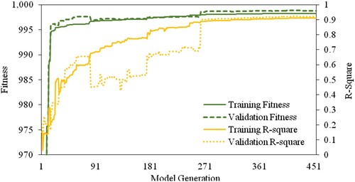
The software developed 454 numbers of sub-models, as demonstrated in Figure 7 when the GEP 20 model accomplished about 40,000 generations. Training and validation fitness suddenly boosted from model 9th. After that, training fitness escalated in a gradual manner. Similarly, validation fitness surged slowly with a fluctuation between the 81st model and the 264th model. On the other hand, training R² moderately amplified until the 264th model, then it forwarded steadily. However, validation R² represents a similar pattern with rapid ups and downs somewhere between the 81st and 264th models. Overall, model 446th fostered the best training R² of 0.911, exploiting the fitness of 998.26. It was also observed that the validation fitness started to decline beyond that model, and training data may be attempting to over-fit. Nonetheless, this study focused on achieving a perfect relationship between the input and output variables; therefore, the prediction accuracy of the 446th model was considered sufficient by assessing the relevant outcomes.

Figure 7. Training and validation Fitness and R² during evolution and model generation.

Expression tree (ET) and prediction equation of best GEP model

This GP model's results were revealed in terms of expression tree (ET) in association with the gene achieved from GEP20, revealed as the best model as the best GEP model for estimating the groove cross-sectional area are illustrated in Table 7.

Table 7. The GEP 20 models’ outcomes in Expression tree’s (ET’s).

Gene	Genetic Expression Tree of model component	Independent variables	Constants evolved
G1			C6 = -9.4198
G2		d2= Subbase Thickness (Tsb) (2)	C0 = 3.1812
		d3= Asphalt Thickness (Ta) (2)	C1 = -9.9348
			C2 = -7.1695
			C4 = 12.7443
			C6 = 4.5184
			C8 = −10.565
			C9 = 7.2017
G3		d0= Pass number (n)(1)	C7 = 9.9188
		d1 = load(L)(1)
		d2= Subbase Thickness (Tsb) (1)
		d3= Asphalt Thickness (Ta) (1)
		d4= Maximum temperature(tmax) (2)
G4		d0= Pass number (n)(3)	C2 = −48.906
		d1 = load(L) (1)	C6 = 6.0061
		d2= Subbase Thickness (Tsb) (1)	C9 = 6.6254
		d3= Asphalt Thickness (Ta) (2)
G5			C7 = 1.8562

Five sub-expression trees with addition as a linking function were achieved. In the ET’s d0, d1, d2, d3, and d4 represents Wheel pass number (n), Wheel load (L), Subbase Thickness (TSB), Asphalt Thickness (T_a), and Maximum temperature (t_max) consecutively. Besides, the numerical constants evolved in different Sub-ETs also highlighted in Table 7.

The final simplified equation expresses the Groove Cross-Sectional Area (f_ga). A mathematical expression, derived from these expression trees of model GEP20, can be listed by the model component as interpreted through the Equation 1(1) $\begin{array}{rl}\text{RMSE}& =\sqrt{\frac{1}{n}\sum _i{(t_i-o_i)}^2}\end{array}$(1) as follows: (1) $\begin{array}{rl}{f}_{ga}& =\\ & \text{Atan}(-9.419)\\ & +\text{Tanh}\left(\sqrt[3]{\text{Max}\left(\begin{array}{c}\left(\text{Max}(\text{d}3,\text{d}2)\text{ x Tanh}(3.181)+\frac{\frac{(-9.935-10.565)}{2}+\frac{(\text{d}2+4.518)}{2}}{2}\right),\\ ((7.202-\text{d}3)\text{x}(-7.169)-12.744)\end{array}\right)}\right)\\ & \text{Tanh}(({(\text{d}4+\text{d}3)}^2+\exp (9.919))+(\text{d}{1}^2-(\text{d}4+\text{d}0)))\ast {\left(\frac{1}{\sqrt[2]{\text{d}2}}\right)}^3\\ & +\text{Exp}(\text{Min}(\text{Atan}\left(\frac{\text{d}0}{6.006}-\frac{\text{d}1+\text{d}0}{2}+\frac{\frac{\frac{-48.906+\text{d}0}{2}+\text{d}3}{2}}{2}\right),\text{Atan}\left(\sqrt[2]{\text{d}3}-\frac{\text{d}2+6.625}{2}\right){)}^3\\ & +\text{Atan}\left(1-\left(1-\frac{1}{1.856}\right)\right)\end{array}$(1) The useful spreadsheet equation is also demonstrated in Equation 2(2) $\begin{array}{rl}\text{MAE}& =\frac{1}{n}\sum _i|t_i-o_i|\end{array}$(2) . (2) $\begin{array}{rl}{f}_{ga}& =ATAN(-9.419)+TANH(POWER(MAX((((MAX(d3,d2)\ast TANH(3.181))\\ & +((((-9.934-10.565)/2)\\ & +((d2+4.518)/2))/2))/2),(((7.201-d3)\ast (-7.169))-12.744)),1/3))\\ & +(TANH(((((d4+d3{)}^2)+EXP(9.919))+((d{1}^2)-(d4+d0))))\ast ((1/(SQRT(d2)){)}^3))\\ & +EXP((MIN(ATAN(((((d0/6.0061)-((d1+d0)/2))\\ & +((((-48.906+d0)/2)+d3)/2))/2)),ATAN((SQRT(d3)-((d2+6.625)/2))){)}^3))\\ & +ATAN((1-(1-(1/(1.856)))))\end{array}$(2) All the input parameters were utilised as observed in the prediction equation, which indicates the input parameters’ importance and relevance to the output. Which ultimately contributes to the precise prediction of the groove closure.

Statistical parameters of the GEP 20 model output

The Statistical parameters of input and output variables in the original dataset and dataset utilised in training, validation and testing phases under the GEP 20 model is expressed in Table 8. The Mean, Median and standard deviation indicate that the set was well distributed in the training, validation and testing phases. Moreover, all input variables’ minimum and maximum values are incorporated in the training phase so that the artificial intelligence techniques accomplish better interpolation during modelling. All of the variables draw quite normal distribution except load (L) that render skewed distribution, which was innate to the original datasets.

Table 8. Statistical parameters of variables in Original, Training, Validation and Testing phases.

			Statistical parameters
Model variables	Phase	N	Min	Max	Mean	Median	Std Dev	Skewness
Pass number (n)	Original All	81	0	37290	13062	11338	10289	0.88
	Training	56	0	37290	13487	11338	10240	0.83
	Validation	13	2310	35508	13051	13258	9281	1.16
	Testing	12	0	37290	11092	7204	12106	1.25
load (L)	Original All	81	55	65	55.74	55	2.635	3.31
	Training	56	55	65	55.71	55	2.599	3.42
	Validation	13	55	65	55.77	55	2.774	3.61
	Testing	12	55	65	55.83	55	2.887	3.46
Subbase Thickness (TSB)	Original All	81	34	39	36.67	37	2.068	−0.24
	Training	56	34	39	36.75	37	2.082	−0.31
	Validation	13	34	39	36.92	37	1.891	−0.57
	Testing	12	34	39	36.00	35.5	2.216	0.36
Asphalt Thickness (Ta)	Original All	81	10	15	12.33	12	2.068	0.24
	Training	56	10	15	12.25	12	2.082	0.31
	Validation	13	10	15	12.08	12	1.891	0.57
	Testing	12	10	15	13.00	13.5	2.216	−0.36
Maximum temperature (tmax)	Original All	81	9	34	25.30	27	7.519	−0.62
	Training	56	9	34	24.59	27	7.589	−0.55
	Validation	13	9	34	26.00	27	8.456	−0.74
	Testing	12	16	34	27.83	29	5.921	−0.77
Groove Cross-Sectional Area Experimental (Y)	Original All	81	0.030	0.070	0.048	0.049	0.006	−0.45
	Training	56	0.030	0.070	0.048	0.049	0.006	−0.39
	Validation	13	0.040	0.060	0.048	0.048	0.004	0.26
	Testing	12	0.040	0.060	0.050	0.052	0.007	−1.21
Groove Cross-Sectional Area Predicted (Model)	Training	56	0.040	0.060	0.048	0.047	0.006	−0.01
	Validation	13	0.040	0.050	0.047	0.047	0.004	−0.27
	Testing	12	0.040	0.060	0.050	0.052	0.005	−1.09

Features of best GEP model

The coefficient of determination (R²) and errors such as RMSE, RAE, and RRSE of training, validating and testing the model GEP 20 are demonstrated in Table 9. The model attained an outstanding fitness of 998.26 for training and 998.80 for validation phases in the full fitness scale of 1000. The coefficient of determination (R²) was obtained at 0.911, 0.921 and 0.924 for training, validation and testing phases. Above all, it is significant that the model was trained, validated, and tested with the same accuracy. The insignificant values of several errors like MAE and RMSE illustrates that the GEP model has been trained well, and it can predict the groove areas with a high degree of accuracy and reliability.

Table 9. R² and errors of training, testing & validating of the model.

Phase	R^2	MAE	RMSE	RAE	RRSE
Training	0.911	0.0012	0.0017	0.3023	0.3002
Validating	0.921	0.0011	0.0012	0.3842	0.2978
Testing	0.924	0.0017	0.0025	0.3243	0.3590

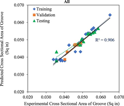
The experimental data plot compared with the predicted results for training, validation and testing phases as ascertained in the GP model is depicted in Figure 8, Figure 9, and Figure 10, respectively. Moreover, the scatter around the line of equality of experimental and predicted groove cross-sectional areas for all data’s are sketched in Figure 11 that acquired R² of 0.906. These scatter plots envisaged the correlation between input variables and derived variables and propagated the preciseness of the model in estimating the prediction values.

Figure 8. Predicted and experimental Groove X-Sectional Area (Training).

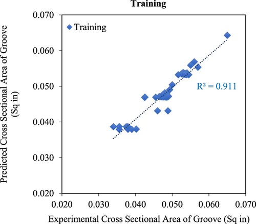
Figure 9. Predicted and experimental Groove X-Sectional Area (Validation).

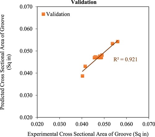
Figure 10. Predicted and experimental Groove X-Sectional Area (Testing).

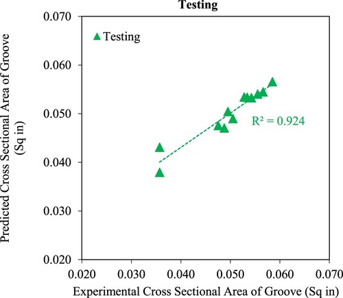
Figure 11. Predicted and experimental Groove X-Sectional Area (All data).

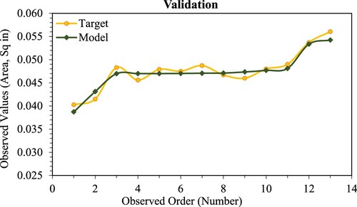
The model sorted fitting curves articulates that the model followed the targeted values quite closely for both the training and validation phases, as illustrated in Figure 12 and Figure 13, respectively.

Figure 12. Model sorted fitting of data (Training phase).

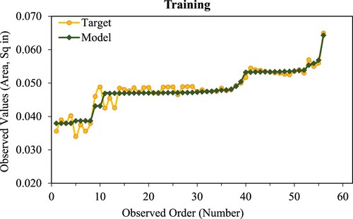
Figure 13. Model sorted fitting of data (Validation phase).

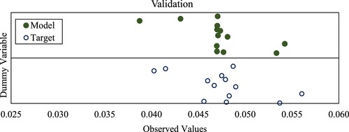
The stacked distributions chart clearly expresses the spread and overlap of the actual and predicted values for both the training and validation phases, as illustrated in Figure 14 and Figure 15 correspondingly. The observed values indicate the grooves cross-sectional area, and the dummy variable is an artificial variable evolved to represent each population number as an attribute with distinct categories. This model fitting chart conveys an aspect of visualisation of the model that helps quick analysis. The stacked distribution expresses that the model output covers the target distribution quite well for both the training and validation phases.

Figure 14. Stacked distribution of data (Training Phase).

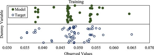
Figure 15. Stacked distribution of data (Validation Phase).

The experimental results evolved by the best model (GEP20) suggest the proficiency of the GEP aptitude in predicting groove cross-sectional area considering the relevant variables.

Relative contribution

The frequency of variables utilised in the GEP models was further investigated by assessing its contribution to fitness in training and validation phases according to the fitness method. As mentioned earlier, GP mainly functions based on the Darwinian principle, which indicates survival of the fittest. Hence, the valuation of each input variable according to the fitness could significantly indicate the importance of each input variable to the output. 113 GEP models with a different frequency of input variables were selected based on R², greater than 0.9, to ensure reliability and accuracy. These selected 113 GEP models are enlisted in Appendix II.

The relative frequency of variables used for each input variable was determined by dividing the individual frequency of variable used by the overall frequency of used variables which indicates the proportion of each input variable in the respective GEP model as illustrated in Appendix III: Stage A. The individual relative frequency of the variables is then multiplied by the fitness that demonstrates the contributions of fitness according to the relative frequency of the variables used in the training phase (Appendix III: Stage B) and validation phase (Appendix III: Stage C), respectively. Finally, the relative importance of the variables was obtained by dividing the individual contribution to the summation of the contribution of fitness as explained in Appendix III: Stage D. The outcomes were ranked in descending order as well.

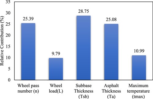
The revealed relative contribution of the input variable in the GEP model is depicted in Figure 16. The most significant input variable was the Subbase Thickness (TSB), which accounts for 28.75% of the contribution and is ranked 1, followed by Wheel pass number (n), comprising 25.39% contribution ranked 2. Afterwards, Asphalt Thickness (Ta) was identified as the following vital variables that constitute 25.08%, ranked 3. However, Wheel load (L) and Maximum temperature (tmax) attained almost the same significance and contribution level with 9.79% and 10.99%, and ranked 4 and 5, respectively. Most importantly, wheel pass number (n) is identified as more important than wheel load (L). In this process, the relative importance of the variables over each other is assessed. Overall, the structural thickness appeared as a significant parameter that dictates the groove closure. Besides, the repetition of the wheel passes also revealed a predominant factor that regulates the degree of groove closure. However, airport authorities can configure their modelling.

Figure 16. Significance and relative contribution of input variables.

Airport authorities can refix and fit the model through calibration depending on their specific construction history, loading characteristics, and frequency. This will provide a general prediction perception of their groove life and term of functional condition. Moreover, the model will effectively reduce the time required to evaluate groove area changes in a similar situation and estimate the rate of deterioration and the per cent of groove closure with respect to aircraft movement. In addition to this, they can plan their budget for future repair and maintenance activities. A detailed field survey is required to determine the state of groove dimension and actual ability to generate friction for final reconstruction or overlay and consecutive groove reinstatement.

The overall results expressed that the GEP model can predict the groove area deterioration close to the experimental results. Furthermore, this GEP model can be an efficient and reliable model for the prediction of groove closure with a high degree of accuracy.

Conclusions

The study has successfully employed GeneXproTools software in modelling the groove deterioration. The R² obtained for training, validation, and testing are 0.911, 0.921 and 0.924, respectively. The results generated from the predictive models fit with the experimental data reasonably well, indicating the accuracy and reliability of the prediction models.

Prior to this, it was difficult to predict the serviceable length of the groove on the runway with certainty. The prediction equation evolved from the GEP model renders valuable information for the prediction of groove area deterioration derived from different input factors like loads, pass number, the thickness of sub-base and Asphalt layer, and temperature. Using GEP, this trendsetting prediction modelling approach, including the statistical analysis, amplified the model's preciseness and can introduce a new chapter in APMS for appropriate groove management and maintaining the required runway frictional performance.

However, there are some factors like rubber contamination on runway grooves, aircraft wheel speed, and variation in materials configuration in runway pavement layer, including inherent characteristics like resilient modulus could be considered for the modelling. More elaborate investigation facilities in operational runways could provide more data for the model calibration and subsequent refinement in future studies.

Finally, this study has developed an innovative and robust model that will enhance the prediction capability for airport authorities on groove closure and groove performance. Therefore, this innovative modelling approach can be integrated into the APMS, which will significantly contribute to runway frictional management by guiding the respective authorities to prepare and execute timely maintenance.

Disclosure statement

No potential conflict of interest was reported by the author(s).

Appendix I: Different Composition of Parameters and Results including Fitness and Errors

Table

Model Type & Run Category: Function Finding Regression
					Gene Domain								Errors
GEP Model No.	Dataset Partitioning (Training & Validation)	Phase	Sample Size (Nos.) & Sampling		Chromosome Number	Head Size	Gene No.	Programme size	Variables Utilised	Generation	Fitness	R^2	RAE	RMSE	MAE	RRSE
GEP	Random Shuffle	Training	64	All	30	8	3	44	5	12889	996.98	0.728	0.4859	0.0030	0.0020	0.5218
1		Validation	9	Odd							995.40	0.564	0.6501	0.0046	0.0032	0.7062
GEP	-do-	Training	63	All	30	8	3	40	5	14590	996.02	0.587	0.7070	0.0040	0.0031	0.6555
2		Validation	9	Even							997.37	0.664	0.7249	0.0026	0.0220	0.7321
GEP	-do-	Training	62	All	30	8	3	36	5	20769	997.13	0.752	0.5161	0.0029	0.0021	0.4987
3		Validation	10	Odd							997.94	0.862	0.3696	0.0021	0.0016	0.3835
GEP	-do-	Training	62	All	30	8	3	36	5	12484	998.14	0.895	0.3772	0.0019	0.0015	0.3264
4		Validation	10	Odd							996.24	0.753	0.4604	0.0038	0.0031	0.5070
GEP	Partition	Training	62	All	30	8	3	36	5	12700	998.50	0.935	0.2602	0.0015	0.0011	0.2677
5		Validation	10	Odd							997.13	0.958	0.5394	0.0029	0.0026	0.5232
GEP	Random Shuffle	Training	61	All	30	8	3	35	5	11121	997.70	0.868	0.3927	0.0023	0.0018	0.3629
6		Validation	10	Even							996.17	0.666	0.8348	0.0018	0.0017	0.7334
GEP	-do-	Training	61	All	36	10	4	67	5	23953	997.92	0.858	0.3759	0.0028	0.0015	0.3766
7		Validation	10	Odd							996.54	0.811	0.4484	0.0032	0.0023	0.4547
GEP	-do-	Training	61	All	36	8	3	38	5	25123	997.33	0.769	0.4915	0.0027	0.0020	0.4831
8		Validation	10	Odd							997.03	0.826	0.4436	0.0030	0.0022	0.4263
GEP	-do-	Training	61	All	48	8	3	42	5	18982	997.37	0.776	0.5092	0.0026	0.0021	0.4741
9		Validation	10	Odd							996.19	0.758	0.6028	0.0038	0.0030	0.5474
GEP	-do-	Training	61	All	48	10	4	45	5	16500	995.66	0.384	0.7898	0.0044	0.0032	0.7870
10		Validation	10	Odd							993.33	0.215	0.8612	0.0067	0.0044	0.9640
GEP	-do-	Training	61	All	30	8	3	36	5	37774	997.98	0.869	0.3906	0.0020	0.0016	0.3651
11		Validation	10	Odd							996.89	0.809	0.4516	0.0031	0.0023	0.4481
GEP	-do-	Training	60	All	30	8	3	39	5	15703	996.54	0.666	0.5322	0.0035	0.0024	0.5869
12		Validation	11	Odd							996.89	0.796	0.4887	0.0031	0.0024	0.4790

All Model: The functions employed included +, −, *, /, Exp, ln, Inverse, x2, 3Rt, Min2, Max2, Avg2, Atan, Tanh, and NOT. (* additional function included Sqrt, and x3)

All Model: The weight of ‘ +, −, *, Avg2' functions was two times that of other functions.

Table

					Gene Domain								Errors
GEP Model No.	Dataset Partitioning (Training & Validation)	Phase	Sample Size (Nos.) & Sampling		Chromosome Number	Head Size	Gene No.	Programme size	Variables Utilised	Generation	Fitness	R^2	RAE	RMSE	MAE	RRSE
GEP	Partition	Training	60	All	30	8	3	39	5	9052	997.05	0.736	0.4454	0.0029	0.0019	0.5178
13		Validation	11	Odd							995.68	0.419	0.8452	0.0043	0.0038	0.8138
GEP	Random Shuffle	Training	59	All	48	8	3	44	5	13319	997.23	0.805	0.4277	0.0028	0.0020	0.4443
14*		Validation	11	Odd							997.84	0.898	0.5380	0.0022	0.0017	0.4664
GEP	-do-	Training	58	Shuffled	48	8	3	41	5	21570	998.19	0.919	0.3079	0.0018	0.0014	0.2929
15*		Validation	11	Odd							997.54	0.891	0.5622	0.0025	0.0018	0.5320
GEP	-do-	Training	57	Shuffled	30	8	3	41	5	45837	998.11	0.896	0.3694	0.0019	0.0015	0.3263
16		Validation	12	Odd							998.40	0.948	0.2778	0.0046	0.0013	0.2665
GEP	-do-	Training	57	Shuffled	45	10	3	48	5	10830	997.01	0.734	0.4913	0.0030	0.0020	0.5196
17		Validation	12	Odd							995.93	0.644	0.5886	0.0041	0.0029	0.6800
GEP	-do-	Training	57	Shuffled	48	12	4	43	4	3966	995.37	0.354	0.8535	0.0046	0.0034	0.8057
18		Validation	12	Odd							995.69	0.597	0.7589	0.0043	0.0037	0.7192
GEP	-do-	Training	56	All	32	8	3	36	5	10588	996.77	0.684	0.4627	0.0037	0.0021	0.5050
19		Validation	13	Odd							996.29	0.745	0.4804	0.0037	0.0029	0.4837
GEP	-do-	Training	56	All	60	14	5	75	5	40687	998.26	0.911	0.3023	0.0017	0.0012	0.3002
20*		Validation	13	Odd							998.80	0.921	0.3842	0.0012	0.0011	0.2978
GEP	-do-	Training	55	Shuffled	30	8	3	41	5	10457	998.22	0.898	0.3533	0.0018	0.0014	0.3192
21		Validation	26	Shuffled							997.76	0.892	0.3629	0.0022	0.0017	0.3671
GEP	-do-	Training	55	Shuffled	30	8	3	39	5	67265	998.21	0.898	0.3518	0.0018	0.0014	0.3185
22		Validation	13	Top half							998.37	0.935	0.3149	0.0016	0.0014	0.2686
GEP	-do-	Training	55	Shuffled	30	8	3	41	5	15960	998.23	0.898	0.3496	0.0018	0.0014	0.3179
23		Validation	13	Shuffled							997.75	0.908	0.2946	0.0011	0.0010	0.2545
GEP	Random Shuffle	Training	55	All	30	8	3	41	5	22007	998.28	0.916	0.3108	0.0017	0.0013	0.2893
24		Validation	13	Top half							998.33	0.925	0.3284	0.0017	0.0014	0.3229
GEP	-do-	Training	55	Shuffled	30	8	3	41	5	51047	998.23	0.899	0.3494	0.0018	0.0014	0.3178
25		Validation	13	Top half							998.38	0.936	0.3132	0.0016	0.0014	0.2679
GEP	-do-	Training	54	Shuffled	48	8	3	41	5	12619	998.35	0.913	0.3091	0.0017	0.0013	0.2998
26		Validation	13	Top half							997.93	0.895	0.4768	0.0021	0.0019	0.4121

All Model: The functions employed included +, −, *, /, Exp, ln, Inverse, x2, 3Rt, Min2, Max2, Avg2, Atan, Tanh, and NOT. (* additional function included Sqrt, and x3).

All Model: The weight of ‘ +, −, *, Avg2' functions was two times that of other functions.

Appendix II. Frequency of variables used and fitness in training and validation phases

Table

		Frequency of variables used in model, fr					Fitness,
Sl No.	Model Number Generated	Wheel pass number (n)	Wheel load(L)	Subbase Thickness (TSB)	Asphalt Thickness (Ta)	Maximum temperature (tmax)	Training (Ft)	Validation (Fv)
1	334	3	1	5	3	2	998.124	998.689
2	335	3	1	5	3	2	998.124	998.689
3	336	3	1	5	3	2	998.127	998.691
4	337	3	2	5	3	2	998.128	998.687
5	338	3	2	5	3	2	998.128	998.687
6	339	3	2	5	3	2	998.128	998.687
7	340	3	1	6	3	2	998.128	998.687
8	341	3	1	5	3	2	998.128	998.687
9	342	4	1	5	3	2	998.128	998.687
10	343	3	1	5	3	2	998.128	998.687
11	344	4	1	5	4	2	998.131	998.722
12	345	4	1	5	4	2	998.133	998.743
13	346	3	1	5	4	2	998.136	998.712
14	347	3	1	5	3	2	998.142	998.679
15	348	3	1	5	3	2	998.143	998.681
16	349	4	1	5	3	2	998.144	998.729
17	350	4	1	5	4	2	998.153	998.730
18	351	4	2	5	3	2	998.160	998.733
19	352	5	2	5	3	2	998.170	998.749
20	353	5	2	5	3	2	998.171	998.746
21	354	5	2	6	3	1	998.171	998.746
22	355	5	2	6	3	1	998.171	998.746
23	356	5	2	5	3	2	998.172	998.738
24	357	5	2	5	3	2	998.173	998.740
25	358	5	2	5	3	2	998.176	998.729
26	359	5	2	5	3	2	998.176	998.729
27	360	5	2	4	3	3	998.176	998.729
28	361	5	2	4	3	4	998.182	998.752
29	362	5	2	4	3	4	998.182	998.752
30	363	5	3	4	3	3	998.183	998.755
31	364	5	2	4	4	1	998.188	998.788
32	365	5	2	4	4	1	998.188	998.751
33	366	5	1	5	4	1	998.192	998.748
34	367	5	1	4	5	1	998.192	998.745
35	368	5	1	4	4	2	998.193	998.747
36	369	5	1	4	4	2	998.193	998.746
37	370	5	1	4	4	2	998.193	998.747
38	371	5	1	5	4	2	998.195	998.755
39	372	5	1	5	4	2	998.195	998.755
40	373	5	1	5	4	2	998.197	998.753
41	374	5	1	4	6	2	998.197	998.752
42	375	4	1	4	7	2	998.198	998.746
43	376	4	1	5	4	3	998.198	998.747
44	377	4	1	4	6	3	998.198	998.747
45	378	4	2	5	4	3	998.207	998.785
46	379	4	2	4	5	3	998.207	998.784
47	380	4	2	4	6	2	998.207	998.783
48	381	4	1	5	5	2	998.207	998.784
49	382	4	1	4	5	3	998.214	998.725
50	383	4	1	4	4	3	998.214	998.772
51	384	4	1	4	4	2	998.216	998.772
52	385	4	1	4	4	2	998.216	998.768
53	386	4	1	4	3	3	998.218	998.767
54	387	4	1	4	3	2	998.219	998.764
55	388	4	1	5	3	1	998.219	998.764
56	389	4	1	5	3	1	998.219	998.764
57	390	4	1	5	3	1	998.219	998.763
58	391	4	1	5	3	1	998.220	998.762
59	392	4	1	5	4	1	998.220	998.762
60	393	4	1	5	4	1	998.221	998.765
61	394	4	1	5	3	1	998.221	998.765
62	395	4	1	6	3	1	998.227	998.780
63	396	4	1	6	3	1	998.227	998.780
64	397	4	1	6	3	2	998.228	998.776
65	398	4	1	7	4	1	998.228	998.775
66	399	4	1	5	5	1	998.228	998.776
67	400	4	1	5	6	1	998.229	998.778
68	401	4	1	5	5	2	998.229	998.777
69	402	4	1	5	5	2	998.229	998.776
70	403	4	1	6	5	1	998.230	998.776
71	404	4	1	6	5	1	998.230	998.776
72	405	5	1	5	4	1	998.233	998.791
73	406	4	1	5	4	2	998.233	998.814
74	407	4	1	5	4	2	998.233	998.814
75	408	4	2	4	4	2	998.238	998.807
76	409	4	2	5	4	2	998.238	998.807
77	410	4	2	5	4	2	998.239	998.801
78	411	4	2	4	4	3	998.242	998.824
79	412	4	2	4	5	2	998.245	998.825
80	413	4	2	4	5	2	998.245	998.823
81	414	4	2	4	5	2	998.245	998.823
82	415	4	3	4	5	1	998.245	998.823
83	416	4	3	4	5	1	998.245	998.823
84	417	4	2	5	5	1	998.248	998.850
85	418	4	2	4	5	1	998.249	998.849
86	419	4	2	4	5	1	998.249	998.849
87	420	4	3	4	5	1	998.250	998.849
88	421	4	3	4	5	1	998.250	998.848
89	422	4	2	5	4	1	998.250	998.848
90	423	4	2	4	4	2	998.250	998.848
91	424	4	2	4	5	2	998.250	998.851
92	425	4	2	6	4	1	998.250	998.851
93	426	4	2	5	4	2	998.255	998.813
94	427	4	2	4	4	2	998.255	998.812
95	428	4	2	4	4	2	998.255	998.812
96	429	5	2	4	4	2	998.255	998.812
97	430	4	3	4	5	1	998.255	998.812
98	431	5	2	4	5	1	998.255	998.812
99	432	4	2	4	6	1	998.256	998.805
100	433	4	2	4	4	3	998.256	998.804
101	434	4	2	4	4	3	998.256	998.804
102	435	4	2	5	4	2	998.256	998.808
103	436	4	2	5	4	2	998.256	998.808
104	437	4	2	4	6	1	998.256	998.808
105	438	4	2	4	5	1	998.256	998.808
106	439	4	2	5	5	1	998.256	998.808
107	440	4	2	5	5	1	998.257	998.812
108	441	4	2	5	5	1	998.257	998.812
109	442	4	3	1	5	1	998.257	998.811
110	443	4	3	4	5	1	998.257	998.804
111	444	4	2	4	5	2	998.257	998.803
112	445	4	2	4	5	2	998.258	998.803
113	446	4	2	4	5	2	998.258	998.802

Appendix III:

sample calculations for evaluating the importance of input variable to output according to contribution of fitness

A. Relative frequency of variables used (r).

Table

		Variables
Sl No.	Model Number	Wheel pass number (n)	Wheel load(L)	Subbase Thickness (Tsb)	Asphalt Thickness (Ta)	Maximum temperature (tmax)
1	334	0.214	0.071	0.357	0.214	0.143
2	335	0.214	0.071	0.357	0.214	0.143
113	446	0.235	0.118	0.235	0.294	0.118

Note: Individual frequency of variables used is divided by the total of frequency of variables used, e.g. (Model 334) r_n= fr_n / (fr_n+ fr_L+ fr_Tsb+ fr_Ta+ fr_t) = 3/ (3 + 1 + 5 + 3 + 2) = 0.214.

B. Contribution of fitness according to relative frequency of variables used in training phase (Ct).

Table

		Variables
Sl No.	Model Number	Wheel pass number (n)	Wheel load(L)	Subbase Thickness (Tsb)	Asphalt Thickness (Ta)	Maximum temperature (tmax)
1	334	213.884	71.295	356.473	213.884	142.589
2	335	213.884	71.295	356.473	213.884	142.589
113	446	234.884	117.442	234.884	293.605	117.442
	Σ	28644.38	11042.39	32424.46	28287.26	12399.20

Note: The individual relative frequency of variable used is multiplied by the fitness in the training phase. e.g. (Model 334) Ct_n = r_n × Ft = 0.214 × 998.124 = 213.884.

C. Contribution of fitness according to relative frequency of variables used in validation phase (Cv).

Table

		Variables
Sl No.	Model Number	Wheel pass number (n)	Wheel load(L)	Subbase Thickness (Tsb)	Asphalt Thickness (Ta)	Maximum temperature (tmax)
1	334	214.005	71.335	356.675	214.005	142.670
2	335	214.005	71.335	356.675	214.005	142.670
113	446	235.012	117.506	235.012	293.765	117.506
	Σ	28660.52	11048.64	32442.72	28303.20	12406.18

Note: The individual relative frequency of variable used is multiplied by the fitness in validation phase e.g. (Model 334) Cv_n = r_n × Fv = 0.214 × 998.689 = 214.005.

D. Relative importance of input variable to output (RI).

Table

	Variables
Phase	Wheel pass number (n)	Wheel load(L)	Subbase Thickness (Tsb)	Asphalt Thickness (Ta)	Maximum temperature (tmax)
Training	25.39	9.79	28.75	25.08	10.99
Validation	25.39	9.79	28.75	25.08	10.99
Rank	2	5	1	3	4

Note: Summation of the contribution of fitness for individual input variable is divided by the summation of the contribution of fitness for all input variables in respective training or validation phase, then multiplies by 100. The relative importance is ranked in descending order.

e.g. RI_n = ΣCt_n/(ΣCt_n+ … + ΣCtt) × 100 = 28644.38/ (28644.38+ … +12399.20) × 100 = 25.39.

References

- Apeagyei, A. K., Al-Qadi, I. L., Ozur, H., & Buttlar, W. G. (2007). Performance of grooved bituminous runway pavement. Center of Excellence for Airport Technology: Technical Report, 28, 1–10.
- Daiutolo, H. (2012, September). Runway Grooving and Skid Resistance. IX ALACPA Seminar of Airport Pavements, Panama City, Panama.
- Di Mascio, P., & Moretti, L. (2019). Implementation of a pavement management system for maintenance and rehabilitation of airport surfaces. Case Studies in Construction Materials, 11, e00251. http://dx.doi.org/10.1016/j.cscm.2019.e00251
- Emery, S. (2005a). Asphalt on Australian airports. In AAPA PAVEMENTS INDUSTRY CONFERENCE, 2005, SURFERS PARADISE, QUEENSLAND, AUSTRALIA.
- Emery, S. (2005b, November). Bituminous surfacing’s for pavement on Australian airports. In Proceedings Australian airports association convention, Hobart.
- Federal Aviation Administration (FAA). (1997). Measurement: Construction and Maintenance of Skid-Resistant Airport Pavement Surfaces. FAA Advisory Circular 150/5320-12C, Washington DC.
- Federal Aviation Administration (FAA). (2010). FAA Grooving Requirements. FAA Worldwide Technology Transfer Conference, New Jersey, USA.
- Federal Aviation Administration (FAA). (2014). Airport Pavement Management Program (PMP). Advisory Circular 150/5380-7B, Federal Aviation Administration, Washington, USA.
- Federal Aviation Administration (FAA). (2016). Measurement and Maintenance of Skid-Resistant Airport Pavement Surfaces. Advisory Circular 150/5320-12D, Federal Aviation Administration, Washington, USA. https://www.faa.gov/documentlibrary/media/advisory_circular/draft-150-5320-12d.pdf
- Fernando, A. K., Shamseldin, A. Y., & Abrahart, R. J. (2009, July). Using gene expression programming to develop a combined runoff estimate model from conventional rainfall-runoff model outputs. In Proc., 18th World IMACS Congress and MODSIM09 International Congress on Modelling and Simulation (pp. 2377–2383).
- Ferreira, C. (2001). Gene expression programming: A new adaptive algorithm for solving problems. Complex Systems, 13(2), 87–129.
- Ferreira, C. (2006). Gene expression programming: Mathematical modeling by an artificial intelligence. 2nd Ed. Springer-Verlag.
- Fwa, T. F., Pasindu, H. R., Ong, G. P., & Zhang, L. (2014). Analytical evaluation of skid resistance performance of trapezoidal runway grooving. In Transportation Research Board 93th Annual Meeting (p. 24).
- Gepsoft. (2020). Gene Expression Programming. Retrieved November 26, 2020 from https://www.gepsoft.com/tutorials/GettingStartedWithRegression.html
- Hajihassani, M., Abdullah, S. S., Asteris, P. G., & Armaghani, D. J. (2019). A gene expression programming model for predicting tunnel convergence. Applied Sciences, 9(21), 4650. https://doi.org/10.3390/app9214650
- Leong, H. Y., Ong, D. E. L., Sanjayan, J. G., Nazari, A., & Kueh, S. M. (2018). Effects of significant variables on compressive strength of soil-fly ash geopolymer: Variable analytical approach based on neural networks and genetic programming. Journal of Materials in Civil Engineering, 30(7), 04018129. https://doi.org/10.1061/(ASCE)MT.1943-5533.0002246
- Nazari, A., Rajeev, P., & Sanjayan, J. G. (2015). Modelling of upheaval buckling of offshore pipeline buried in clay soil using genetic programming. Engineering Structures, 101, 306–317. https://doi.org/10.1016/j.engstruct.2015.07.013
- Pasindu, H. R. (2020). Analytical evaluation of impact of groove deterioration on runway frictional performance. Transportation Research Procedia, 48, 3814–3823. https://doi.org/10.1016/j.trpro.2020.08.038
- Patterson, J. W. (2012). Evaluation of trapezoidal runway grooving. FAA-TC-TN12/7, Federal Aviation Administration, Washington, DC.
- Pham, V. N., Oh, E., & Ong, D. E. (2021). Gene-Expression programming-based model for estimating the compressive strength of cement-fly ash stabilized soil and parametric study. Infrastructures, 6(12), 181. https://doi.org/10.3390/infrastructures6120181
- Safaei, F., & Hintz, C. (2014, June). Investigation of the effect of temperature on asphalt binder fatigue. In International Society for Asphalt Pavement Conference (pp. 1491-1500).
- Shahmansouri, A. A., Bengar, H. A., & Ghanbari, S. (2020). Compressive strength prediction of eco-efficient GGBS-based geopolymer concrete using GEP method. Journal of Building Engineering, 31, 101326. https://doi.org/10.1016/j.jobe.2020.101326
- Tarawneh, B. (2018). Gene expression programming model to predict driven pipe piles set-up. International Journal of Geotechnical Engineering. https://doi.org/10.1080/19386362.2018.1460964
- timeanddate. (2020). temperature data at weather in New Jersey. Retrieved November 23, 2020 from available at https://www.timeanddate.com/weather/@5101760/historic?month=6&year=2016
- Valle, P. D., & Thom, N. (2020). Pavement layer thickness variability evaluation and effect on performance life. International Journal of Pavement Engineering, 21(7), 930–938. https://doi.org/10.1080/10298436.2018.1517873
- Wang, Q., & Larkin, A. (2019). Asphalt pavement groove life analysis at the FAA national airport pavement test facility. In Al-Qadi, H. Ozer, A. Loizos, & S. Murrell (Eds.), Airfield and highway pavements 2019: Innovation and sustainability in highway and airfield pavement technology (pp. 418-426). Reston: American Society of Civil Engineers. https://doi.org/10.1061/9780784482476.041
- White, G. (2017). Managing skid resistance and friction on asphalt runway surfaces. In World Conference on Pavement and Asset Management, Milan, Italy.
- White, G., & Rodway, B. (2014). Distress and maintenance of grooved runway surfaces. Airfield Engineering and Maintenance Summit.