On the role of pressure in elasto-inertial turbulence

Abstract

The dynamics of elasto-inertial turbulence is investigated numerically from the perspective of the coupling between polymer dynamics and flow structures. In particular, direct numerical simulations of channel flow with Reynolds numbers ranging from 1000 to 6000 are used to study the formation and dynamics of elastic instabilities and their effects on the flow. Based on the splitting of the pressure into inertial and polymeric contributions, it is shown that the polymeric pressure is a non-negligible component of the total pressure fluctuations, although the rapid inertial part dominates. Unlike Newtonian flows, the slow inertial part is almost negligible in elasto-inertial turbulence. Statistics on the different terms of the Reynolds stress transport equation also illustrate the energy transfers between polymers and turbulence and the redistributive role of pressure. Finally, the trains of cylindrical structures around sheets of high polymer extension that are characteristics of elasto-inertial turbulence are shown to be correlated with the polymeric pressure fluctuations.

Keywords:

• elasto-inertial turbulence
• FENE-P
• maximum drag reduction
• DNS
• pressure split

1. Introduction

Polymer additives are known for producing upward of 80% drag reduction in turbulent wall-bounded flows through strong alteration and reduction of turbulent activity [1]. The changes in flow dynamics induced by polymers do not lead to flow relaminarisation but, atmost, to a universal asymptotic state called maximum drag reduction (MDR) [2]. At the same time, polymer additives have also been shown to promote transition to turbulence [3], or even lead to a chaotic flow at very low Reynolds number as in elastic turbulence [4,5].

These seemingly contradictory effects of polymer additives can be explained by the interaction between elastic instabilities and the flow’s inertia characterising elasto-inertial turbulence, hereafter referred to as EIT [6,7]. EIT is a state of small-scale turbulence driven by elastic instabilities that exists by either creating its own extensional flow patterns or by exploiting extensional flow topologies. EIT could provide answers to phenomena that current understanding of MDR cannot, such as the absence of a log-law in finite-Reynolds numbers MDR flows [8,9], and the phenomenon of early turbulence. Moreover, it supports De Gennes’ picture [10] that drag reduction derives from two-way energy transfers between turbulent kinetic energy of the flow and elastic energy of polymers at small scales, resulting in an overall modification of the turbulence energy cascade at high Reynolds numbers.

As shown by viscoelastic pipe experiments and direct numerical simulations [6,7], an elastic instability can occur at a Reynolds number smaller than the transition in Newtonian pipe flow if the polymer concentration and Weissenberg number are sufficiently large. Moreover, it is observed that the skin friction coefficient C_f = τ_w/(1/2ρU_b²), where ρ is the density, U_b the bulk velocity and τ_w the wall shear stress, then follows the characteristic MDR friction law, as shown in Figure 1. Visualisations of numerical simulations indicate that thin sheets of locally high polymer stretch, tilted away from the wall and elongated in the flow direction, create trains of spanwise cylindrical structures of alternating sign (see Figure 2). In low-elasticity flows, EIT is drown out by the canonical Newtonian near-wall vortices. At higher elasticity, the polymer drag reduction mechanism inhibits Newtonian vortices and EIT dominates. It is hypothesised that EIT may be an asymptotic state of parallel wall-bounded flows over a large range of Reynolds numbers.

Figure 1. Skin friction coefficient C_f as a function of the Reynolds number Re_H for two Weissenberg numbers, Wi_H = 4 (

) and Wi_H = 30 (

). Lines indicate correlations for laminar (· · · · · · · ·, C_f = 12/Re_H) and turbulent (– – – –, C_f = 0.073Re^{− 1/4}_H [11]) Newtonian channel flow, and for MDR (——, C_f = 0.42Re^{− 0.55}_H [12]); Newtonian solutions are also included (). Unlike for Newtonian flows, the skin friction of viscoelastic flows at sufficiently high Weissenberg number departs from the laminar correlation at subcritical Reynolds number and then smoothly transitions to the MDR asymptote.

Figure 2. Contour of the normalised polymer extension C_ii/L on selected planes and instantaneous isosurface of the second invariant Q_A of the velocity gradient tensor in the lower half of the channel for the subcritical case Re_H = 1000 and Wi_H = 4; Q_A = 0.1 (red) and Q_A = −0.1 (cyan). Trains of mostly spanwise cylindrical Q_A structures of alternating sign form around thin sheets of large polymer extension.

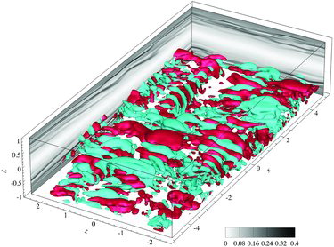
It is suggested that the formation of sheets of polymer stretch results from the unstable nature of the nonlinear advection of low-diffusivity polymers [7]. These sheets, hosting a significant increase in extensional viscosity, create a strong local anisotropy, with a formation of local low-speed jet-like flow. The response of the flow is through pressure, whose role is to redistribute energy across components of momentum, resulting in the formation of waves, or trains of alternating rotational and straining motions. Once triggered, EIT is self-sustained since the elastic instability creates the very velocity fluctuations it feeds upon.

The underlying mechanism driving EIT is here further investigated through an analysis of the pressure, and its interaction with topological structures of the flow and polymer stress. The approach relies on the splitting of the pressure into inertial and polymeric contributions [13–15]. Additionally, energy transfers between polymers and turbulence are further analysed through statistics on the different terms of the Reynolds stress transport equation.

The paper is organised as follows. Section 2 describes the numerical simulations and the corresponding parameters, and summarises the main theoretical aspects regarding the splitting of the pressure. Results are then presented in Section 3. Finally, the key findings are summarised and discussed in Section 4.

2. Method

2.1. Direct numerical simulations

Channel flow simulations are performed in a Cartesian domain, where x, y and z are the streamwise, wall-normal and spanwise directions, respectively. For a polymer solution, the non-dimensional equations governing the flow are the continuity equation, , where is the velocity vector, and the momentum equation, (1) The Reynolds number is based on the bulk velocity U_b, the full channel height H = 2h and the kinematic viscosity ν of the solution, Re_H = U_bH/ν. The polymer stress tensor is computed using the FENE-P model [16]: (2) where is the unit tensor and is the polymer conformation tensor, whose transport equation is (3) The properties of the polymer solution are the ratio β of solvent viscosity to the zero-shear viscosity of the solution, the maximum polymer extension L (so that C_ii < L²) and the Weissenberg number Wi_H = λU_b/H based on the solution relaxation time λ and the integral time scale H/U_b. The Weissenberg number can also be defined as , where is the wall shear-rate of the corresponding Newtonian flow at each Reynolds number.Equations (1(1) )–(3(3) ) are solved using finite differences on a staggered grid and a semi-implicit time advancement scheme [17,18]. After a thorough resolution study, a domain size of 10h × 2h × 5h with 256 × 151 × 256 computational nodes was chosen. All results have been verified on domains with a factor 2 in horizontal dimensions and a factor 2 in resolution in each direction. The CFL number was set to 0.15 to guarantee the boundedness of .

Three different viscoelastic and one Newtonian cases are considered here, as summarised in Table 1. The lower Reynolds number corresponds to a subcriticalflow (Re_H < Re_{H, c}, where Re_{H, c} = 1719 defines the intersection between the laminar and MDR friction drag lines as shown in Figure 1), while the larger Reynolds number corresponds to a value for which the Newtonian flow is turbulent. The Weissenberg numbers at Re_H = 6000 are chosen to achieve high drag reduction (HDR) and MDR, respectively. For all three viscoelastic cases, L = 200 and β = 0.9 were used. The corresponding statistics can be found in [7].

Table 1. Parameters used for the three viscoelastic and the Newtonian cases considered here. For all simulations, the FENE-P model is used with the maximum polymer extension parameter L = 200 and β = 0.9.

ReH^a	Reh^b	h^+^c	WiH^d	Wih^e	Wi^+^f	DM [%]^g	Colour^h
1000	500	40	4	8	24	+7
6000	3000	130	4	8	96	−56
6000	3000	120	30	60	720	−61
6000	3000	190	–	–	–	0

^aReynolds number based on the bulk velocity U_b and the total channel height H.

^bReynolds number based on the bulk velocity U_b and the channel half-height h (for comparison with previous publications).

^cChannel half-height h normalised by the friction velocity and the viscosity ν.

^dWeissenberg number based on the solution relaxation time λ and the integral time scale H/U_b.

^eWeissenberg number based on the solution relaxation time λ and the integral time scale h/U_b (for comparison with previous publications).

^fWeissenberg number based on the solution relaxation time λ and the wall-shear rate of the corresponding Newtonian case.

^g Drag modification (reduction or increase) measured as the relative change of the skin friction coefficient with the comparable Newtonian flow friction coefficient (laminar or turbulent).

^h Colour scheme used throughout the paper for each specific case.

2.2. Inertial and polymeric contributions to pressure

In order to investigate the role of pressure in the mechanism underlying EIT, a similar approach to Mansour et al. [13], Kim [14] and Ptasinski et al. [15] is followed. Taking the divergence of the momentum equation (1(1) ) leads to a Poisson equation for the pressure: (4) where Q_A = (− 1/2)∂_iu_j∂_ju_i = (− 1/2)∂_i∂_ju_iu_j is the second invariant of the velocity gradient tensor. In contrast to a Newtonian flow, a second term appears on the right-hand side, which represents the contribution from the polymeric stress. For a periodic channel flow, the pressure satisfies Equation (4(4) ) with the boundary conditions (5) at the walls and periodicity in x and z.

By splitting the right-hand side of Equation (4(4) ) into different terms and separating the effect of the wall boundary condition, their respective contributions to the total pressure can be isolated. In particular, we consider here following splitting for the pressure fluctuations : (6) where fluctuations are denoted by •′ and mean quantities by . The first three contributions on the right-hand side of Equation (6(6) ) are solutions of [19]: (7) (8) (9) with the homogeneous wall boundary conditions (10) The ‘rapid inertial’ part, p′_r, is linear in the velocity fluctuations and represents the immediate response to a change imposed on the mean field, while the ‘slow inertial’ part, p′_s, feels this change through nonlinear interactions [14]. In addition to these two inertial terms, the pressure in a viscoelastic flow also has an elastic contribution, p′_p, originating in the polymeric stress. Finally, the effect of the wall boundary condition is represented by the Stokes pressure, p′_St, which satisfies (11) with the inhomogeneous boundary conditions (12) As the Stokes pressure is typically much smaller than the other contributions, it is not considered here.

This pressure split is applied to the simulation results for the four cases mentioned above and statistics are computed in order to identify the relative contributions from inertia and elasticity, as shown below.

3. Results

Equations (7(7) )–(9(9) ) have been solved with homogeneous wall boundary conditions to obtain the three contributions p′_r, p′_s and p′_p. About 250 fields have been collected for each of the four cases considered, on which statistics have been performed as a function of the wall-normal coordinate y⁺. The + exponent indicates wall units, i.e., a normalisation by the friction velocity and viscosity ν.

3.1. Statistics

3.1.1. Pressure fluctuations

The root-mean-square (rms) values of the different pressure contributions and of their sum across the channel height are shown in Figure 3.The most striking observation is that the level of pressure fluctuations at Re_H = 6000 remains almost constant, or even slightly increases at the wall and at the centre of the channel, when the Weissenberg number is increased, i.e., when the turbulence is damped (Figure 3(a)). This differs markedly from the velocity fluctuations, which strongly decrease with drag reduction (see Figures 1 and 2 in [7]). Pressure fluctuations are, however, much lower in the subcritical case (Re_H = 1000).

Figure 3. Pressure rms as a function of y⁺. (a) Total pressure for the Newtonian case at Re_H = 6000 (

), and the viscoelastic cases Re_H = 1000, Wi_H = 4 (

); Re_H = 6000, Wi_H = 4 (HDR,

); and Re_H = 6000, Wi_H = 30 (MDR,

). (b)–(d) Pressure contributions for selected cases: p′_r ( — · — ); p′_s (· · · · · · · ·); p′_p ( – – – – ); p′_rs = p′_r + p′_s ( ——— ); p′_rsp = p′_r + p′_s + p′_p (

).

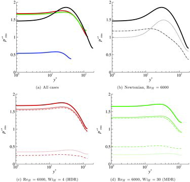
The qualitative behaviour is different between Newtonian and viscoelastic flows. In particular, the rms profile is much flatter in the latter case. The splitting of the pressure shows that the marked peak in the pressure fluctuations seen in the buffer layer for the Newtonian case originates in the slow pressure (see Figure 3(b)). Figure 3(b) and 3(c) demonstrates that polymers strongly damp the slow pressure contribution while the rapid part slightly increases, which explains the flatter profiles in the viscoelastic cases.The dominating contribution comes thus from the rapid pressure in contrast to a Newtonian turbulent channel flow, where the slow part dominates almost everywhere [19]. This result differs from the analysis of Ptasinski et al. [15], who found that slow and rapid contributions are more or less equal at MDR. However, their simulation was performed at a much lower Weissenberg number and with a lower maximum extensibility parameter than the present calculations.

The elastic pressure, absent in the Newtonian case, has a non-negligible and increasing contribution when the Weissenberg number is increased. If the Weissenberg number is high enough, this polymeric contribution is larger than the slow part. This is not the case here at HDR (Figure 3(c)) where both rapid and slow parts are larger than for the MDR case, owing to the stronger turbulence.

Figure 4(a) shows the ratio of the rms of the elastic pressure p′_p to the inertial pressure, p′_rs = p′_r + p′_s, indicating that the polymer contribution is about 15% of p′_rs at Wi_H = 4 and increases to about 35%–40% at the larger Weissenberg number. The ratio of the polymeric to inertial pressure contributions also remains quite constant in the near-wall region. The ratio of the rms of the slow pressure p′_s to the inertial pressure, p′_rs is shown in Figure 4(b). This ratio also remains rather flat with only a slight increase towards the channel centre. The slow part is only about 6% and 20% of the inertial pressure at Re_H = 1000 and Re_H = 6000, respectively.

Figure 4. (a) Ratio of the polymeric p′_p to the inertial p′_rs pressure rms as a function of y⁺. (b) Ratio of the slow p′_s to the inertial p′_rs pressure rms as a function of y⁺. Same colour labels as in Figure 3.

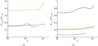
It is interesting to notice that the ratio of the polymeric part to the inertial part seems to depend mostly on the Weissenberg number, while the ratio of the slow part to the inertial part appears to depend on the Reynolds number. This is, however, only speculative and more cases need to be analysed. Moreover, the splitting into an inertial and elastic contribution is a simplified view as the polymer stress in Equation (1(1) ) can create velocity fluctuations and, thus, indirectly contributes to the inertial pressure and conversely, as discussed below.

3.1.2. Reynolds stress transport

Dubief et al. [7] suggested that the role of pressure is to redistribute turbulent kinetic energy across components of momentum, resulting in the formation of waves, or trains of alternating rotational and straining motions. To illustrate this, various terms in the transport equation for the Reynolds stress , and, in particular, for the components of the turbulent kinetic energy (no summation is implied on the subscript α) are further analysed: (13) where is the production term, the transport term, ε_ij the dissipation term and the polymer body force.

The last term in Equation (13(13) ) represents the creation of Reynolds stress due to polymer stress fluctuations. It can be separated into two contributions: (14) The first term on the right-hand side is in the divergence form and thus corresponds to the transport of Reynolds stress by fluctuating polymer stress. The second term, , is the polymer stress work. In particular, represents the transfer of energy between the mean turbulent kinetic energy and the mean elastic energy of the polymers [7,20]. This term can be either positive or negative, and a positive value corresponds to an energy transfer from the polymers to the turbulence.

Similarly, the velocity–pressure gradient correlation (15) can be separated into two contributions, Π_ij = Φ_ij + d^(p)_ij, representing the pressure–strain and the pressure–diffusion, respectively [19]. They are defined as (16) (17)

Taking half the trace of Equation (13(13) ) leads to the transport equation for the turbulent kinetic energy k. In the case of a fully developed channel flow, the only contribution to is the streamwise component . The pressure–diffusion term, d^(p)_ii, is in the divergence form and thus represents a transport term. On the other hand, Φ_ii is deviatoric and thus does not contribute to changes in k, but merely redistributes the turbulent kinetic energy across the components. In particular, in a Newtonian channel flow, turbulent kinetic energy is produced from the mean shear through ; this energy is then redistributed from to and through the terms Φ_αα.

This well-known picture changes, however, in the viscoelastic case. In particular, the terms offer a new path for the production of k, i.e., the transfer of energy from the polymers to the turbulence. Moreover, this term does not solely contribute to , but to all three components.

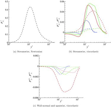
Figure 5 shows the production terms for the diagonal components of the Reynolds stress tensor. Compared to a Newtonian flow, the production term is much lower in a drag-reduced flow (see Figure 5(a) and 5(b)). Nevertheless, the most interesting aspect is that the streamwise transfer of energy from the polymers to the turbulence, , dominates. In other words, the turbulence is mainly sustained by the polymers, as already recognised in previous studies [7,18,20]. On the other hand, the polymer production for the two other components of the diagonal is negative (see Figures 5(c)), indicating a transfer of energy from the flow to the polymers. The transfer rates are, however, 10 times lower than for the streamwise component. It is also interesting to see that has almost the same level for both HDR and MDR, while all other production terms are much lower at MDR.

Figure 5. (a) and (b) Streamwise production terms ( – – – – ) and ( ——— ) as a function of y⁺. The polymer contribution is positive, indicating a transfer of energy from the polymers to the turbulence. (c) Wall-normal and spanwise production terms ( · · · · · · · · ) and ( — · — ) as a function of y⁺. In this case, energy is transferred from the turbulence to the polymers, but the levels are much lower than in the streamwise direction. Same colour labels as in Figure 3.

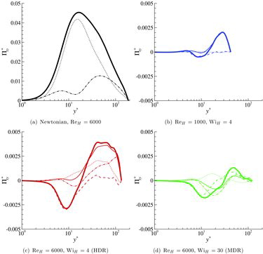
The analysis above indicates that energy is transferred from the polymers to the flow through the streamwise component, and that a small portion of this energy goes back to the polymers through the wall-normal and spanwise components. The redistribution of energy from to and is achieved through the pressure–strain term Φ_ij. The different components of the diagonal, Φ_αα, are shown in Figures 6–8. Their qualitative behaviour is very similar to a Newtonian flow at a similar Reynolds number [19], but with lower levels owing to the turbulence reduction. One can observe that Φ_xx is negative while Φ_yy and Φ_zz are positive for y⁺ ≳ 10, which demonstrates the redistribution of energy from the streamwise component to both the wall-normal and spanwise components. Note, however, that Φ_xx is negative and Φ_yy positive very close to the wall. Similar conclusions can be drawn from Π_ij and (not shown here).

Figure 6. Streamwise pressure–strain component Φ⁺_xx as a function of y⁺ obtained from the different pressure contributions: p′_r ( — · — ); p′_s ( · · · · · · · · ); p′_p ( – – – – ); p′_rs = p′_r + p′_s (———); p′_rsp = p′_r + p′_s + p′_p (

). Same colour labels as in Figure 3. Φ_xx is negative in most of the domain indicating an energy transfer away from the streamwise component.

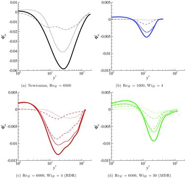
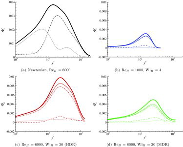
Unlike for Newtonian flows, the largest contribution to the pressure-strain term comes from the rapid part, and a non-negligible contribution from the polymer part is observed. The polymeric contribution is comparatively larger for Φ_yy and lower for Φ_zz, which tends to indicate that the elastic contribution slightly favours a two-dimensional flow, the three-dimensionality being mostly driven by the inertial part. On the other hand, the slow part is very weak, except for Φ_yy at HDR in the centre of the channel. Interestingly, the behaviour of the rapid contribution to Φ_yy differs between the Newtonian and the viscoelastic cases (see Figure 7). In the Newtonian case, it is positive in the near-wall region and then becomes negative for y⁺ ≳ 10; in the viscoelastic case, it is exactly the opposite. Actually, the rapid contribution in the viscoelastic case behaves exactly like the slow contribution in the Newtonian case.

Figure 7. Wall-normal pressure–strain component Φ⁺_yy as a function of y⁺ obtained from different pressure contributions. Same line style as in Figure 6 and same colour labels as in Figure 3. Φ_yy is positive in most of the domain indicating an energy transfer to the wall-normal component.

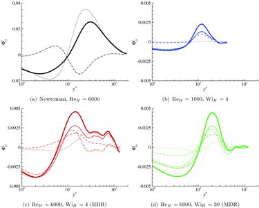
Figure 8. Spanwise pressure–strain component Φ⁺_zz as a function of y⁺ obtained from the different pressure contributions. Same line style as in Figure 6 and same colour labels as in Figure 3. Φ_zz is positive everywhere indicating an energy transfer to the spanwise component.

The Reynolds shear stress production is shown in Figure 9. The same qualitative behaviour is observed for Newtonian and viscoelastic flows, but with a lower magnitude in drag-reduced flows due to the reduction of turbulence intensity by polymers. is negative, indicating that Reynolds shear stress is produced. However, this production of Reynolds shear stress is compensated by a positive polymer contribution through . The lower magnitude of the production term and this cancelling effect between and explains the very low levels of Reynolds shear stress seen in MDR flows (see Figure 2 of [7]).

Figure 9. Production terms ( – – – – ) and ( ——— ) of Reynolds shear stress as a function of y⁺. Same colour labels as in Figure 3. Both terms cancel each other in the viscoelastic cases, explaining the very low levels of Reynolds shear stress observed.

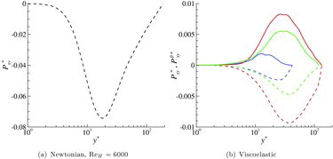
A difference between Newtonian and viscoelastic flows is also observed for the x − y component of the velocity–pressure gradient correlation. In particular, Π_xy in the viscoelastic cases is negative (i.e., production of Reynolds shear stress) around y⁺ ≈ 10, which is not observed in the Newtonian case (see Figure 10). This behaviour is directly caused by the polymer pressure contribution p′_p.

Figure 10. Pressure–strain component Π⁺_xy as a function of y⁺ obtained from the different pressure contributions: p′_r ( — - — ); p′_s (· · · · · · · ·); p′_p ( – – – – ); p′_rs = p′_r + p′_s ( ——— ); p′_rsp = p′_r + p′_s + p′_p (

). Same colour labels as in Figure 3.

3.2. Instantaneous fields

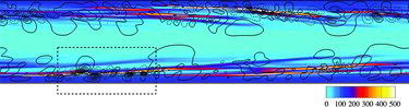
As shown in Figure 2, the flow is characterised by trains of cylindrical Q_A structures of alternating sign around thin sheets of large polymer extension. This is further illustrated in Figure 11, which shows the contour of the polymer stress component T_xx and isolines of Q_A in an plane for the lower Reynolds number case. The long thin sheets of large polymer extension surrounded by cylindrical structures are clearly visible.

Figure 11. Instantaneous contour of the polymer stress component T_xx and isolines of Q_A (dash lines represent negative values) in an plane for Re_H = 1000 and Wi_H = 4. The flow is from left to right and the dashed box represents the region plotted in the next two figures.

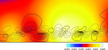
A small region of the plane around one of these sheets (indicated by the dashed box in Figure 11) is shown in Figures 12 and 13. The first figure shows the instantaneous contour of the polymeric pressure contribution p_p and isolines of Q_A, and illustrates the strong correlation between these two quantities. The largest fluctuations of p_p are of alternating sign and located on each side of the sheet, mostly in between cylindrical Q_A structures. The wavelength of these structures is the same as the wavelength of the Q_A structures. On the other hand, the inertial pressure p_rs does not show such a clear correlation. Large fluctuations of p_rs are rather correlated with the centre of strong Q_A structures, as shown in Figure 13. In particular, as in inertial turbulence, positive values of Q_A correspond to low pressure regions, and thus, to vortical regions [21]. The analysis of the polymer body force (not shown here) indicates that the polymer body force is mostly parallel to the sheet with opposite sign on each side. Additionally, also alternates direction along the sheet with the same wavelength as the Q_A structures and opposite sign, indicating that the polymers are most likely the driving force that creates these structures.

Figure 12. Instantaneous contour of the polymeric pressure contribution p_p and isolines of Q_A (dash lines represent negative values) in an plane for Re_H = 1000 and Wi_H = 4. The region plotted corresponds to the dashed box in Figure 11. A clear correlation between p_p and Q_A is visible.

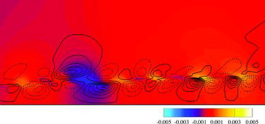
Figure 13. Instantaneous contour of the inertial pressure contribution p_rs and isolines of Q_A (dash lines represent negative values) in an plane for Re_H = 1000 and Wi_H = 4. The region plotted corresponds to the dashed box in Figure 11. Unlike the previous figure, no clear correlation between p_rs and Q_A is visible.

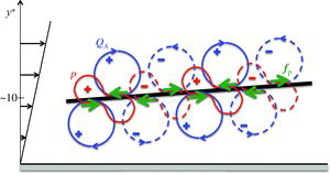
The overall picture gained from this analysis is schematically summarised in Figure 14. It is believed that the combined effect of advection at low diffusivity and existing flow perturbations leads to the formation of sheets of high polymer extension and, in turn, to a large increase in the extensional viscosity, and thus in the polymer stress. Small perturbations of the sheets cause the polymer body force to alternate direction, and thereby, create these cylindrical Q_A structures. The pressure adapts to ensure zero divergence of the velocity and redistribute part of the turbulent kinetic energy from the streamwise to the other components. Once triggered, this process appears to be self-sustained, at least over the hundreds of flow through-time simulated here. Therefore, it can be conjectured that these characteristic trains of cylindrical structures are mostly driven by the polymers. Nonetheless, an indirect effect from inertia probably also contributes to the dynamics. Finally, note that, since the present analysis is based on correlations, these causal connections are only speculative. Further analysis is still required to ascertain this.

Figure 14. Schematics of the typical structures observed around thin sheets of large polymer extension (black line) in the near-wall region: second invariant of the velocity gradient tensor Q_A (blue), pressure p (red) and polymer body force (green). Dotted lines indicate a negative value.

4. Conclusion and future work

A new state of small-scale turbulence, elasto-inertial turbulence, has been recently discovered in polymeric solutions. EIT has not only provided answers to previously unexplained phenomena such as early turbulence [6,22], it is also a unique window into the creation of turbulence by means other than those known in Newtonian turbulence. The current understanding of EIT is that it is driven by both inertial and elastic instabilities, leading to strong alterations of the flow dynamics compared to the Newtonian case. In particular, the flow departs from the laminar solution at a Reynolds number lower than the transitional Reynolds number observed for a Newtonian fluid. The topology of coherent structures identified by the second invariant Q_A of the velocity gradient tensor is dramatically different than the coherent structures observed in Newtonian near-wall turbulence. Interestingly, our simulations show that EIT coherent structures extend to larger Reynolds numbers where the skin friction reaches the MDR asymptotic law. The spatial organisation of regions of highly stretch polymers is also found to be similar between and 6000. In this context, the present analysis aimed at better characterising the dynamics of EIT and, in particular, to study the role of pressure in the relationship between the Q_A structures and the organisation of polymer stretch.

The splitting of the pressure into different components, in particular, into an elastic and an inertial part, has provided a tool to assess the relative contributions of both components to the overall dynamics. It is shown that the elastic, or polymer, pressure is a non-negligible component of the total pressure fluctuations, although the rapid part dominates. Unlike Newtonian flows, the slow part is much lower in elasto-inertial turbulence. Statistics also demonstrate the redistributive role of pressure, transferring energy from the streamwise to the other components. Finally, a schematic description of the typical structures encountered in EIT is proposed. It is postulated that those small-scale structures, associated with thin sheets of large polymer extension, are directly driven by the polymers. Nonetheless, an indirect inertial contribution is still possible, and most likely required for self-sustaining dynamics.

In a broader context, elasto-inertial turbulence offers a new perspective on the interaction between polymers and flow. First, its existence at Re = 1000, for which the Newtonian flow is laminar, clearly establishes a pathway of energy from polymers to flow, lending support to De Gennes’ theory of energy transfers between polymers and flow [10]. Then, the existence of EIT at larger Reynolds number raises some questions as to its role in MDR and the nature of MDR, which will be addressed in future publications.

Many questions remain unanswered, such as the mechanism by which small perturbations of the sheet lead to a body force of alternating sign, the role of those elastic instabilities, the validity of the above conclusions at larger Reynolds numbers, the two-dimensional nature of these instabilities. Finally, the possible existence of EIT in other flows, specifically non-wall-bounded flows, remains a speculation based on our current definition: EIT occurs in parallel flows with a mean shear. Consequently, one may anticipate that EIT may live in shear flows (mixing layers, jets) or in a Kolmogorov flow. Further analysis is thus required to obtain a definite description of the physical mechanisms underlying EIT, which will be part of future work.

Additional information

Funding

V.E. Terrapon acknowledges the financial support of a Marie Curie FP7 Career Integration Grant [grant number PCIG10-GA-2011-304073) and of a grant from the ‘Fonds Spéciaux pour la Recherche’ of the University of Liege (Crédits classiques 2013) [grant number C-13/19]. The Vermont Advanced Computing Center is gratefully acknowledged for providing the computing resources. Y. Dubief acknowledges the support from the National Institutes of Health [grant number P01HL46703 (project 1]. J. Soria acknowledges the support of the Australian Research Council [grant number DP1095620]. This work was initiated during the Center for Turbulence Research 2012 Summer Program.

Notes

1. In laminar flows, , so that Wi⁺ = 6Wi_H.

2. The Newtonian flow is laminar.

3. Note that .

4. The subcritical case (not shown here) is qualitatively similar to the MDR case but with lower values.

References

- C.M. White and M.G. Mungal, Mechanics and prediction of turbulent drag reduction with polymer additives, Annu. Rev. Fluid Mech. 40 (2008), pp. 235–256.
- P.S. Virk, H.S. Mickley, and K.A. Smith, The ultimate asymptote and mean flow structure in Toms’ phenomenon, J. Appl. Mech. 37 (1970), pp. 488–493.
- J.W. Hoyt, Laminar-turbulent transition in polymer solutions, Nature 270 (1977), pp. 508–509.
- A. Groisman and V. Steinberg, Elastic turbulence in a polymer solution flow, Nature 405 (2000), pp. 53–55.
- V. Steinberg, Elastic stresses in random flow of a dilute polymer solution and the turbulent drag reduction problem, C. R. Phys. 10 (2009), pp. 728–739.
- D. Samanta, Y. Dubief, M. Holzner, C. Schšfer, A.N. Morozov, C. Wagner, and B. Hof, Elasto-inertial turbulence, Proc. Natl. Acad. Sci. 110 (2013), pp. 10557–10562.
- Y. Dubief, V.E. Terrapon, and J. Soria, On the mechanism of elasto-inertial turbulence, Phys. Fluids 25 (2013), 110817.
- C.M. White, Y. Dubief, and J. Klewicki, Re-examining the logarithmic dependence of the mean velocity distribution in polymer drag reduced wall-bounded flow, Phys. Fluids 24 (2012), 021701.
- B.R. Elbing, M. Perlin, D.R. Dowling, and S.L. Ceccio, Modification of the mean near-wall velocity profile of a high-Reynolds number turbulent boundary layer with the injection of drag-reducing polymer solutions, Phys. Fluids 25 (2013), 085103.
- P.G. De Gennes, Introduction to Polymer Dynamics, Cambridge University Press, Cambridge, 1990.
- R.D. Dean, Reynolds number dependence of skin friction and other bulk flow variables in two-dimensional rectangular duct flow, J. Fluids Eng. 100 (1978), pp. 215–222.
- P.S. Virk, E.W. Merrill, H.S. Mickley, K.A. Smith, and E.L. Mollo-Christensen, The Toms phenomenon: Turbulent pipe flow of dilute polymer solutions, J. Fluid Mech. 30 (1967), pp. 305–328.
- N.N. Mansour, J. Kim, and P. Moin, Reynolds-stress and dissipation-rate budgets in a turbulent channel flow, J. Fluid Mech. 194 (1988), pp. 15–44.
- J. Kim, On the structure of pressure fluctuations in simulated turbulent channel flow, J. Fluid Mech. 205 (1989), pp. 421–451.
- P.K. Ptasinski, B.J. Boersma, F.T.M. Nieuwstadt, M.A. Hulsen, B.H.A.A. van den Brule, and J.C.R. Hunt, Turbulent channel flow near maximum drag reduction: Simulations, experiments and mechanisms, J. Fluid Mech. 490 (2003), pp. 251–291.
- R.B. Bird, R.C. Armstrong, and O. Hassager, Dynamics of Polymeric Liquids. Vol. 2: Kinetic Theory, Wiley-Interscience, 1987.
- Y. Dubief, C.M. White, V.E. Terrapon, E.S.G. Shaqfeh, P. Moin, and S.K. Lele, On the coherent drag-reducing and turbulence-enhancing behaviour of polymers in wall flows, J. Fluid Mech. 514 (2004), pp. 271–280.
- Y. Dubief, V.E. Terrapon, C.M. White, E.S.G. Shaqfeh, P. Moin, and S.K. Lele, New answers on the interaction between polymers and vortices in turbulent flows, Flow Turbul. Combust. 74 (2005), pp. 311–329.
- G.A. Gerolymos, D. Sénéchal, and I. Vallet, Wall effects on pressure fluctuations in turbulent channel flow, J. Fluid Mech. 720 (2013), pp. 15–65.
- V. Dallas, J.C. Vassilicos, and G.F. Hewitt, Strong polymer-turbulence interactions in viscoelastic turbulent channel flow, Phys. Rev. E 82 (2010), 066303.
- Y. Dubief and F. Delcayre, On coherent-vortex identification in turbulence, J. Turbul. 1 (2000) pp. 1–22.
- Y. Dubief, C.M. White, E.S.G. Shaqfeh, and V.E. Terrapon, Polymer Maximum Drag Reduction: A Unique Transitional State, Center for Turbulence Research Annual Research Briefs, Stanford, CA, 2010.