Controlling Rayleigh–Bénard convection via reinforcement learning

Abstract

Thermal convection is ubiquitous in nature as well as in many industrial applications. The identification of effective control strategies to, e.g. suppress or enhance the convective heat exchange under fixed external thermal gradients is an outstanding fundamental and technological issue. In this work, we explore a novel approach, based on a state-of-the-art Reinforcement Learning (RL) algorithm, which is capable of significantly reducing the heat transport in a two-dimensional Rayleigh–Bénard system by applying small temperature fluctuations to the lower boundary of the system. By using numerical simulations, we show that our RL-based control is able to stabilise the conductive regime and bring the onset of convection up to a Rayleigh number $R{a}_c\approx 3\cdot {10}^4$, whereas state-of-the-art linear controllers have ${\mathrm{Ra}}_c\approx {10}^4$. Additionally, for $\mathrm{Ra}>3\cdot {10}^4$, our approach outperforms other state-of-the-art control algorithms reducing the heat flux by a factor of about 2.5. In the last part of the manuscript, we address theoretical limits connected to controlling an unstable and chaotic dynamics as the one considered here. We show that controllability is hindered by observability and/or capabilities of actuating actions, which can be quantified in terms of characteristic time delays. When these delays become comparable with the Lyapunov time of the system, control becomes impossible.

Keywords:

• Reinforcement learning
• Thermal convection
• Rayleigh–Bénard
• Control
• Chaos

1. Introduction

Rayleigh–Bénard convection (RBC) provides a widely studied paradigm for thermally driven flows, which are ubiquitous in nature and in industrial applications [1]. Buoyancy effects, ultimately yielding to fluid dynamics instability, are determined by temperature gradients [2] and impact on the heat transport. The control of RBC is an outstanding research topic with fundamental scientific implications [3]. Additionally, preventing, mitigating or enhancing such instabilities and/or regulating the heat transport is crucial in numerous applications. Examples include crystal growth processes, e.g. to produce silicon wafers [4]. Indeed, while the speed of these processes benefits from increased temperature gradients, the quality of the outcome is endangered by fluid motion (i.e. flow instability) that grows as the thermal gradients increase. Thus the key problem addressed here: can we control and stabilise fluid flows that, due to temperature gradients, would otherwise be unstable?

In the Boussinesq approximation, the fluid motion in RBC can be described via the following equations [5]: (1) $\begin{array}{rl}\frac{\mathrm{\partial }\mathbf{u}}{\mathrm{\partial }t}+\mathbf{u}\cdot \mathrm{\nabla }\mathrm{\nabla }\mathbf{u}& =-\mathrm{\nabla }\mathrm{\nabla }p+\nu {\mathrm{\nabla }}^2\mathbf{u}+\hat{\mathbf{y}}\alpha g(T-T_0),\end{array}$(1) (2) $\begin{array}{rl}\frac{\mathrm{\partial }T}{\mathrm{\partial }t}+\mathbf{u}\cdot \mathrm{\nabla }\mathrm{\nabla }T& =\kappa {\mathrm{\nabla }}^{2}T,\end{array}$(2) where t denotes the time, $\mathbf{u}$ the incompressible velocity field ($\mathrm{\nabla }\mathrm{\nabla }\cdot \mathbf{u}=0$), p the pressure, ν the kinematic viscosity, α the thermal expansion coefficient, g the magnitude of the acceleration of gravity (with direction $\hat{\mathbf{y}}$), $T_0$ a reference temperature and κ the thermal diffusivity. For a fluid system confined between two parallel horizontal planes at distance H and with temperatures $T_C$ and $T_H=T_C+\mathrm{\Delta }T$, respectively for the top and the bottom element ($\mathrm{\Delta }T>0$), it is well known that the dynamics is regulated by three non-dimensional parameters: the Rayleigh and Prandtl numbers and the aspect ratio of the cell (i.e. the ratio between the cell height and width $L_x$), i.e. (3) $\mathrm{Ra}=\frac{g\alpha (T_H-T_C)H^3}{\kappa \nu },\mathrm{Pr}=\nu /\kappa ,\mathrm{\Gamma }=H/L_x.$(3) Considering adiabatic side walls, a mean heat flux, q, independent on the height establishes on the cell: (4) $q={\overline{⟨u_{y}T⟩}}_x-\kappa {\mathrm{\partial }}_y{\overline{⟨T⟩}}_x=\mathrm{const},$(4) where $⟨\cdot {⟩}_x$ indicates an average with respect to the x-axis, parallel to the plates, and $\overline{\bullet }$ the time averaging. The time-averaged heat flux is customarily reported in a non-dimensional form, scaling it by the conductive heat flux, $\kappa \mathrm{\Delta }T/H$, which defines the Nusselt number (5) $\mathrm{Nu}=\frac{q}{\kappa \mathrm{\Delta }T/H}.$(5) As the Rayleigh number overcomes a critical threshold, $\mathrm{Ra}{}_c$, fluid motion is triggered enhancing the heat exchange ($\mathrm{Nu}>1$).

Dubbed in terms of Rayleigh and Nusselt numbers, our control question becomes: can we diminish, or minimise, Nusselt for a fixed Rayleigh number?

In recent years, diverse approaches have been proposed to tackle this issue. These can be divided into passive and active control methods. Passive control methods include: acceleration modulation [3,6], oscillating shear flows [7] and oscillating boundary temperatures [8]. Active control methods include: velocity actuators [9] and perturbations of the thermal boundary layer [10–12]. Many of these methods, although ingenious, are not practical due, e.g. to the requirement of a perfect knowledge of the state of the system or a starting condition close to the conductive state – something difficult to establish [11]. Another state-of-the-art active method, that is used in this paper as comparison, is based on a linear control acting at the bottom thermal boundary layer [13]. The main difficulty in controlling RBC resides in its chaotic behaviour and chaotic response to controlling actions. In recent years, Reinforcement Learning (RL) algorithms [14] have been proven capable of solving complex control problems, dominating extremely hard challenges in high-dimensional spaces (e.g. board games [15,16] and robotics [17]). RL is a supervised Machine Learning (ML) [18] approach aimed at finding optimal control strategies. This is achieved by successive trial-and-error interactions with a (simulated or real) environment which iteratively improve an initial random control policy. Indeed, this is usually a rather slow process which may take millions of trial-and-error episodes to converge [19].

RL has been applied in the physical sciences [20] and used in connection with fluid flows [21], such as for training smart inertial or self-propelling particles [22–24], for schooling of fishes [25,26], soaring of birds and gliders in turbulent environments [27,28], optimal navigation in turbulent flows [29,30], drag reduction by active control in the turbulent regime [31] and more [32–37].

In this work, we show that RL methods can be successfully applied for controlling a Rayleigh–Bénard  system at fixed Rayleigh number reducing (or suppressing) convective effects. Considering a 2D proof-of-concept setup, we demonstrate that RL can significantly outperform state-of-the-art linear methods [13] when allowed to apply (small) temperature fluctuations at the bottom plate (see setup in Figure 1). In particular, we target a minimization of the time-averaged Nusselt number (Equation 5(5) $\mathrm{Nu}=\frac{q}{\kappa \mathrm{\Delta }T/H}.$(5) ), aiming at reducing its instantaneous counterpart: (6) ${\mathrm{Nu}}_{\mathrm{instant}}(t)=\frac{⟨u_{y}T{⟩}_{x,y}-\kappa {\mathrm{\partial }}_y⟨T{⟩}_{x,y}}{\kappa \mathrm{\Delta }T/H},$(6) where the additional average along the vertical direction, y, amends instantaneous fluctuations.

Figure 1. Schematics of linear (a) and Reinforcement Learning (b) control methods applied to a Rayleigh–Bénard  system and aiming at reducing convective effects (i.e. the Nusselt number). The system consists of a domain with height, H, aspect ratio, $\mathrm{\Gamma }=1$, no-slip boundary conditions, constant temperature $T_C$ on the top boundary, adiabatic side boundaries and a controllable bottom boundary where the imposed temperature $T_B(x,t)$ can vary in space and time (according to the control protocol) while keeping a constant average $⟨T_B(x,t){⟩}_x=T_H$. Because the average temperature of the bottom plate is constant, the Rayleigh number is well defined and constant over time. The control protocol of the linear controller (a) works by calculating the distance measure $E(x,t)$ from the ideal state (cf. Equation 10(10) ${\hat{T}}_B(x,t)=\mathcal{R}({\tilde{T}}_B(x,t))=-\mathcal{R}((k_P-k_D{\mathrm{\partial }}_t)E(x,t))$(10) –11(11) $E(x,t)=⟨u_y(x,y,t){⟩}_y/V_0,$(11) ) and, based on linear relations, applies temperature corrections to the bottom plate. The RL method (Figure 1b) uses a Neural Network controller which acquires flow state from a number of probes at fixed locations and returns a temperature profile (see details in Figure 2). The parameters of the Neural Network are automatically optimised by the RL method, during training. Moreover, in the RL case, the temperature fluctuations at the bottom plate are piece-wise constant and can have only prefixed temperature value between two states, hot or cold (cf. Equation 12(12) ${\tilde{T}}_k\in \{C,-C\}.$(12) ). Operating with discrete actions reduces significantly the complexity and the computational resources needed for training.

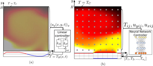
Figure 2. Sketch of the neural network determining the policy adopted by the RL-based controller (policy network, π, cf. Figure 1(b) for the complete setup). The input of the policy network is a state vector, $\mathbf{s}$, which stacks the values of temperature and both velocity components for the current and the previous D−1 = 3 timesteps. Temperature and velocity are read on an evenly spaced grid of size $G_X=8$ by $G_Y=8$. Hence, $\mathbf{s}$ has dimension $n_f\cdot G_X\cdot G_Y\cdot D=3\cdot 8\cdot 8\cdot 4=768$. The policy network π is composed of two fully connected feed forward layers with $n_{\mathrm{neurons}}=64$ neurons and $\sigma (\cdot )=\text{tanh}(\cdot )$ activation. The network output is provided by one fully connected layer with $\sigma (\cdot )=\varphi (\cdot )$ activation (Equation 16(16) $y_k=\varphi (z_k)=\frac{1}{1+\exp (-z_k)},k=1,2,\dots ,n_s$(16) ). This returns the probability vector $\mathbf{y}=[y_1,y_2,\dots ,y_{n_s}]$. The kjth bottom segment has temperature C with probability $y_k$ (Equation 17(17) ${\pi }_k({\tilde{T}}_k=+C|s_i)=\mathrm{Bernoulli}(p=y_k).$(17) ). This probability distribution gets sampled to produce a proposed temperature profile $\tilde{\mathbf{T}}=({\tilde{T}}_1,{\tilde{T}}_2,\dots ,{\tilde{T}}_{n_s})$. The final temperature fluctuations ${\hat{T}}_1,{\hat{T}}_2,\dots ,{\hat{T}}_{n_s}$ are generated with the normalization step in Equation (A7(A7) $\begin{array}{rl}& {\hat{T}}_B(x,t)=\frac{{\tilde{T}}_B^{″}(x,t)}{\underset{x^{\prime }}{max}(1,|{\tilde{T}}_B^{″}(x,t)|/C)}.\end{array}$(A7) ) (cf. Equations (7(7) $T_H=⟨T_B(x,t){⟩}_x,$(7) ) and (9(9) ${\hat{T}}_B(x,t)|\le C\mathrm{\forall }x,t,$(9) )). The temperature profile obtained is applied to the bottom plate during a time interval $\mathrm{\Delta }t$ (control loop), after which the procedure is repeated.

Finding controls fully stabilising RBC might be, however, at all impossible. For a chaotic system as RBC, this may happen, among others, when delays in controls or observation become comparable with the Lyapunov time. We discuss this topic in the last part of the paper employing RL to control the Lorenz attractor, a well-known, reduced version of RBC [38].

The rest of this manuscript is organised as follows. In Section 2, we formalise the Rayleigh–Bénard  control problem and the implementation of both linear and RL controls. In Section 3, we present the control results and comment on the induced flow structures. In Section 4, we analyse physical factors that limit the RL control performance. The discussion in Section 5 closes the paper.

2. Control-based convection reduction

In this section, we provide details of the Rayleigh–Bénard  system considered, formalise the control problem and introduce the control methods.

We consider an ideal gas ($\mathrm{Pr}=0.71$) in a two-dimensional Rayleigh–Bénard  system with $\mathrm{\Gamma }=1$ at an assigned Rayleigh number (cf. sketch and $(x,y)$ coordinate system in Figure 1). We assume the four cell sides to satisfy a non-slip boundary condition, the lateral sides to be adiabatic, and a uniform temperature, $T_C$, imposed at the top boundary. We enforce the Rayleigh number by specifying the average temperature, (7) $T_H=⟨T_B(x,t){⟩}_x,$(7) at the bottom boundary (where $T_B(x,t)$ is the instantaneous temperature at location x of the bottom boundary). Temperature fluctuations with respect to such average, (8) ${\hat{T}}_B(x,t)=T_B(x,t)-T_H,$(8) are left for control.

We aim at controlling ${\hat{T}}_B(x,t)$ to minimise convective effects, which we quantify via the time-averaged Nusselt number (cf. Equation 5(5) $\mathrm{Nu}=\frac{q}{\kappa \mathrm{\Delta }T/H}.$(5) ). We further constrain the allowed temperature fluctuations to (9) ${\hat{T}}_B(x,t)|\le C\mathrm{\forall }x,t,$(9) to prevent extreme and nonphysical temperature gradients (in similar spirit to the experiments in [11]).

We simulate the flow dynamics through the Lattice–Boltzmann method (LBM) [5] employing a double lattice, respectively for the velocity and for the temperature populations (with D2Q9 and D2Q4 schemes on a square lattice with sizes $N_x=N_y$; collisions are resolved via the standard BGK relaxation). We opt for the LBM since it allows for fast, extremely vectorizable, implementations which enables us to perform multiple (up to hundreds) simulations concurrently on a GPU architecture. See Table 1 for relevant simulation parameters; further implementation details are reported in Appendix 1.

Table 1. Rayleigh–Bénard  system and simulation parameters.

Parameters
$\mathrm{Ra}$	${10}^3\stackrel{}{\to }{10}^7$	Rayleigh Number
$\mathrm{Pr}$	0.71	Prandtl Number
Γ	1	Aspect Ratio
Control
C	0.75	Control amplitude limit, Equation (9(9) ${\hat{T}}_B(x,t)|\le C\mathrm{\forall }x,t,$(9) )
$\mathrm{\Delta }t$	$16\stackrel{}{\to }180$	Control loop (unit: LBM steps)
$t_i$	0 (training)	Start evaluation time, for averages in Equation (5(5) $\mathrm{Nu}=\frac{q}{\kappa \mathrm{\Delta }T/H}.$(5) )
”	$150\mathrm{\Delta }t$ (test)	”
$t_e$	$500\mathrm{\Delta }t$	End evaluation time, for averages in Equation (5(5) $\mathrm{Nu}=\frac{q}{\kappa \mathrm{\Delta }T/H}.$(5) )
Lattice Boltzmann simulation (Appendix 1)
$N_X=N_Y$	$20\stackrel{}{\to }350$	Grid size
$c_s^2$	1/3	Speed of sound
τ	0.56	Relaxation time
$T_C$	1	Top boundary temperature
$T_H$	2	Bottom boundary mean temperature
${\tau }_T$	$(\tau -1/2)/\mathrm{Pr}+1/2$	Temperature relaxation time
ν	$c_s^2(\tau -1/2)$	Kinematic viscosity
κ	$(2{\tau }_T-1)/4$	Thermal diffusivity
$\alpha g$	$\mathrm{Ra}{\displaystyle \frac{\kappa \nu }{(T_H-T_C)N_Y^3}}$	Effective gravity

Starting from a system in a (random) natural convective state (cf. experiments [11]), controlling actions act continuously. Yet, to limit learning computational costs, ${\hat{T}}_B(x,t)$ is updated with a period, $\mathrm{\Delta }t$ (i.e. control loop), longer than the LBM simulation step and scaling with the convection time, $t_{\mathrm{convection}}\sim H/U_{\mathrm{bulk}}$. We report in Table A1 the loop length, which satisfies, approximately, $\mathrm{\Delta }t\approx 1/20t_{\mathrm{convection}}$, and the system size, all of which are Ra-dependent. Once more, for computational efficiency reasons, we retain the minimal system size that enables us to quantify the (uncontrolled) Nusselt number within $5\mathrm{\%}$ error (Appendix 1).

In the following sections, we provide details on the linear and RL-based controls.

2.1. Linear control

We build our reference control approach via a linear proportional-derivative (PD) controller [13]. Our control loop prescribes instantaneously the temperature fluctuations at the bottom boundary as (10) ${\hat{T}}_B(x,t)=\mathcal{R}({\tilde{T}}_B(x,t))=-\mathcal{R}((k_P-k_D{\mathrm{\partial }}_t)E(x,t))$(10) with $k_P$, $k_D$ being constant parameters and the (signed) distance from the optimal conductive state ($u_x=u_y=0$), $E(x,t)$, satisfying (11) $E(x,t)=⟨u_y(x,y,t){⟩}_y/V_0,$(11) where $V_0$ is a reference vertical velocity. To ensure the constraints given by Equations (7(7) $T_H=⟨T_B(x,t){⟩}_x,$(7) ), (9(9) ${\hat{T}}_B(x,t)|\le C\mathrm{\forall }x,t,$(9) ) we operate a clipping and renormalization operation, $\mathcal{R}(\cdot )$, as described in Appendix 2.

Various other metrics, $E(x,t)$, have been proposed leveraging, for instance, on the shadow graph method ($E(x,t)=(⟨\rho (x,y,t){⟩}_y-{\rho }_0)/{\rho }_0$ [11]), and on the mid-line temperature ($E(x,t)=(T(x,H/2,t)-T_{1/2})/\mathrm{\Delta }T$, with $T_{1/2}=1/2(T_H+T_C)$, [10]). These metrics provide similar results and, in particular, an average Nusselt number for the controlled systems within $5\mathrm{\%}$. In this paper, we limit ourselves to a proof of concept for the application of RL to control RB convection, without pretending to show optimality against all other possible linear or non-linear controls, hence we limit our scope to state-of-the-art linear controls. We opted for Equation (11(11) $E(x,t)=⟨u_y(x,y,t){⟩}_y/V_0,$(11) ) as it proved to be more stable. Note that, by restricting to $k_D=0$, one obtains a linear proportional (P) controller. While supposedly less powerful than a PD controller, in our case the two show similar performance. The controller operates with the same space and time discretization of the LBM simulations, with the time derivative of $E(x,t)$ calculated with a first-order backwards scheme. We identify the Rayleigh-dependent parameters $k_P$ and $k_D$ via a grid-search algorithm [39] for $\mathrm{Ra}\le 3\cdot {10}^6$ (cf. values in Table 2). In case of higher $\mathrm{Ra}$, due to the chaoticity of the system, we were unable to find parameters consistently reducing the heat flux with respect to the uncontrolled case.

Table 2. Parameters used for the linear controls in Lattice Boltzmann units (cf. Equation (10(10) ${\hat{T}}_B(x,t)=\mathcal{R}({\tilde{T}}_B(x,t))=-\mathcal{R}((k_P-k_D{\mathrm{\partial }}_t)E(x,t))$(10) ); note: a P controller is obtained by setting $k_D=0$ ). At $\mathrm{Ra}={10}^7$ we were unable to find PD controllers performing better than P controllers, which were anyway ineffective.

		P control	PD control
Ra	$N_x=N_y$	$k_P$	$k_P$	$k_D$
$1\cdot {10}^3$	20	0.0	0.0	0.0
$3\cdot {10}^3$	20	$3.16\cdot {10}^2$	$3.16\cdot {10}^2$	0.0
$1\cdot {10}^4$	20	$4.12\cdot {10}^2$	$5.28\cdot {10}^2$	$8.24\cdot {10}^4$
$3\cdot {10}^4$	25	$8.97\cdot {10}^2$	$5.45\cdot {10}^4$	$1.91\cdot {10}^6$
$1\cdot {10}^5$	30	16.4	94.8	$1.05\cdot {10}^4$
$3\cdot {10}^5$	40	9.38	11.5	$1.87\cdot {10}^3$
$1\cdot {10}^6$	100	6.61	$1.84\cdot {10}^4$	$3.06\cdot {10}^5$
$3\cdot {10}^6$	200	7.38	0.12	31.8
$1\cdot {10}^7$	350	0.33	–	–

2.2. Reinforcement learning-based control

In an RL context, we have a policy, π, that selects a temperature fluctuation, $\hat{T}(x,t)$, on the basis of the observed system state. π is identified automatically through an optimization process, which aims at maximising a reward signal. In our case, we define the system state, the allowed controlling actions and the reward are as follows:

• The state space, S, includes observations of the temperature and velocity fields (i.e. of $n_f=3$ scalar fields) probed on a regular grid in $G_X\times G_Y=8\times 8$ nodes for the last D = 4 time steps (i.e. $t,t-\mathrm{\Delta }t,\dots ,t-(D-1)\mathrm{\Delta }t$, where t is the current time). Note that the probe grid has a coarser resolution than the lattice, i.e. $G_X<N_X$, $G_Y<N_Y$, which allows to reduce the complexity of the control problem. It holds, therefore, $S={\mathbb{R}}^{D\cdot n_f\cdot G_X\cdot G_Y}$.

• The action space, A, includes the temperature profiles for the lower boundary that the controller can instantaneously enforce. We allow profiles which are piece-wise constant functions on $n_s=10$ segments (cf. Figure 1). Moreover, each of the $n_s$ function elements, ${\tilde{T}}_k$ ($k=1,2,\dots ,n_s$), can attain only two temperature levels, i.e. (12) ${\tilde{T}}_k\in \{C,-C\}.$(12) To enforce the constraint in Equation (7(7) $T_H=⟨T_B(x,t){⟩}_x,$(7) ), (9(9) ${\hat{T}}_B(x,t)|\le C\mathrm{\forall }x,t,$(9) ), we normalise the profile according to Appendix 2, generating the final profile ${\hat{T}}_k=\mathcal{R}({\tilde{T}}_k)$. After normalization, the action space includes $2^{n_s}-1$ distinct actions. While allowing for discontinuous temperature profiles is unrealistic, it enables a significant reduction of the computational complexity and the search difficulty in the action search space. We deem that RL algorithms would be capable of finding suitable control strategies also when applied in experiments with continuous temperature profiles, possibly after longer training, due to their inherent flexibility. Furthermore, as far as the physics is concerned, a discontinuous control in time/space or a continuous implementation with frequencies and wavelengths high enough to fall in the dissipative-turbulent ranges should nevertheless be equivalent.

• The reward function defines the goal of the control problem. We define the reward, $r_{l+1}$, as the negative instantaneous Nusselt number (cf. Equation 6(6) ${\mathrm{Nu}}_{\mathrm{instant}}(t)=\frac{⟨u_{y}T{⟩}_{x,y}-\kappa {\mathrm{\partial }}_y⟨T{⟩}_{x,y}}{\kappa \mathrm{\Delta }T/H},$(6) ) which results from applying a temperature profile $a_l\in A$ at time $t_l$. In formulas, it holds (13) $r_{l+1}=-{\mathrm{Nu}}_{\mathrm{instant}}(t_{l+1}).$(13) Note that the RL controller aims at maximising the reward accumulated over time (rather than the instantaneous reward), which minimises the average Nusselt number, Equation (5(5) $\mathrm{Nu}=\frac{q}{\kappa \mathrm{\Delta }T/H}.$(5) ), as desired.

We employ the Proximal Policy Optimization (PPO) RL algorithm [40], which belongs to the family of Policy Gradient Methods. Starting from a random initial condition, Policy Gradient Methods search iteratively (and probabilistically) for optimal (or sufficient) policies by gradient ascent (based on local estimates of the performance). Specifically, this optimization employs a probability distribution, $\pi (a_i|s_i)$, on the action space conditioned to the instantaneous system state. At each step of the control loop, we sample and apply an action according to the distribution $\pi (a|s)$. Notably, the sampling operation is essential at training time, to ensure an adequate balance between exploration and exploitation, while at test time, this stochastic approach can be turned deterministic by restricting to the action with highest associated probability. In our case, at test time we used the deterministic approach for $\mathrm{Ra}<3\cdot {10}^6$ and the stochastic approach for $\mathrm{Ra}\ge 3\cdot {10}^6$, as this allowed for higher performance.

The PPO algorithm is model free, i.e. it does not need assumptions on the nature of the control problem. Besides, it does not generally require significant hyperparameter tuning, as often happens for RL algorithms (e.g. value-based method [40]). Due to a lack of standard hyperparameters for flow control, the hyperparameters employed are based on the work on RL for games by Burda et al. [41]. See Appendix 3 for the specific values.

When the state vector $s_i$ is high dimensional (or even continuous), it is common to parameterise the policy function in probabilistic terms as $\pi (a_i|s_i)=\pi (a_i|s_i;\mathit{\theta })$, for a parameter vector $\mathit{\theta }$ [15]. This parameterization can be done via different kinds of functions and, currently, neural networks are a popular choice [42]. In the simplest case, as used here, the neural network is a multilayer perceptron [14] (MLP) which is often used in RL [41]. An MPL is a fully connected network in which neurons are stacked in layers and information flows in a pre-defined direction from the input to the output neurons via ‘hidden’ neuron layers. The ith neuron in the $(n+1)$th layer operates returning the value $h_i^{(n+1)}$, which satisfies (14) $h_i^{(n+1)}=\sigma (b_i^{(n)}+\sum _j{A}_{ij}^{(n)}{h}_j^{(n)}),$(14) where the $h_j^{(n)}$'s are the outputs of the neurons of the previous layer (the nth one), which thus undergo an affine transformation via the matrix $A_{ij}^{(n)}$ and the biases $b_i^{(n)}$. The non-linear activation function σ provides the network with the capability of approximating non-linear functions [42]. During training, the parameters $\mathit{\theta }$ get updated through back propagation [43] (according to the loss defined by the PPO algorithm) which results in progressive improvements of the policy function.

To increase the computational efficiency, we opt for a policy function factorised as follows: (15) $\pi (a_i|s_i)=\pi ({\tilde{T}}_1,{\tilde{T}}_2,\dots ,{\tilde{T}}_{n_s}|s_i)=\prod _{k=1}^{n_s}{\pi }_k\left({\tilde{T}}_k\right|s_i).$(15) In other words, we address the marginal distributions of the local temperature values ${\tilde{T}}_1,{\tilde{T}}_2,\dots ,{\tilde{T}}_{n_s}$. We generate the marginals by an MLP (with two hidden layers each with $\sigma (\cdot )=\text{Tanh}(\cdot )$ activation) that has $n_s$ final outputs, $y_1,y_2,\dots ,y_{n_s}$, returned by sigmoid activation functions, in formulas: (16) $y_k=\varphi (z_k)=\frac{1}{1+\exp (-z_k)},k=1,2,\dots ,n_s$(16) with $z_k=\sum _j{A}_{kj}^{(2)}{h}_j^{(2)}+b_k^{(2)}$ (see Figure 2, note that $0\le \varphi (z_k)\le 1$). The values $y_1,y_2,\dots ,y_{n_s}$ provide the parameters for $n_s$ Bernoulli distributions that determine, at random, the binary selection between the temperature levels $\{-C,C\}$. In formulas, it holds (17) ${\pi }_k({\tilde{T}}_k=+C|s_i)=\mathrm{Bernoulli}(p=y_k).$(17) The final temperature profile is then determined via Equation (12(12) ${\tilde{T}}_k\in \{C,-C\}.$(12) ) and the normalization in Equation (A5(A5) $\begin{array}{rl}& {\tilde{T}}_B^{\prime }(x,t)=\text{Clip}({\tilde{T}}_B(x,t),-C,C)\end{array}$(A5) ). We refer to Figure 2 for further details on the network.

3. Results

We compare the linear and RB-based control methods on nine different scenarios with Rayleigh number ranging between $\mathrm{Ra}={10}^3$ (just before the onset of convection) and $\mathrm{Ra}={10}^7$ (mild turbulence, see Table A1). Figure 3 provides a summary of the performance of the methods in terms of the (ensemble) averaged Nusselt number. Until $\mathrm{Ra}\approx {10}^4$, the RL control and state-of-the-art linear control deliver similar performance. At higher Ra numbers, in which the Rayleigh–Bénard  system is more complex and chaotic, RL controls significantly outperform linear methods. This entails an increment of the critical Rayleigh number, which increases from $\approx {10}^3$, in the uncontrolled case, to $\approx {10}^4$, in case of linear control, and to $\approx 3\cdot {10}^4$ in case of RL-based controls. Above the critical Rayleigh, RL controls manage a reduction of the Nusselt number which remains approximately constant, for our specific experiment, it holds ${\mathrm{Nu}}_{\mathrm{uncontrolled}}-{\mathrm{Nu}}_{\mathrm{RL}}\approx 2.5\mathrm{for}\mathrm{Ra}<3\cdot {10}^6.$ In contrast, the linear method scores only ${\mathrm{Nu}}_{\mathrm{uncontrolled}}-{\mathrm{Nu}}_{\mathrm{linear}}\approx 1.5\mathrm{for}\mathrm{Ra}<{10}^6,$ while at higher Rayleigh it results completely ineffective.

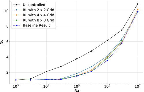
Figure 3. Comparison of Nusselt number, averaged over time and ensemble, measured for uncontrolled and controlled Rayleigh–Bénard  systems (note that all the systems are initialised in a natural convective state). We observe that the critical Rayleigh number, $\mathrm{Ra}{}_c$, increases when we control the system, with $\mathrm{Ra}{}_c={10}^4$ in case of state-of-the-art linear control and ${\mathrm{Ra}}_c=3\cdot {10}^4$ in case of the RL-based control. Furthermore, for $\mathrm{Ra}>{\mathrm{Ra}}_c$, the RL control achieves a Nusselt number consistently lower than what measured in case of the uncontrolled system and for state-of-the-art linear controls (P and PD controllers have comparable performance at all the considered Rayleigh numbers, see also [13]). The error bars are estimated as ${\mu }_{\mathrm{Nu}}/\sqrt{N}$, where N = 161 is the number of statistically independent samplings of the Nusselt number.

The reduction of the average Nusselt number is an indicator of the overall suppression – or the reduction – of convective effects, yet it does not provide insightful and quantitative information on the characteristics of the control and of the flow. In Figure 4, we compare the controls in terms of the time histories of the (ensemble-averaged) Nusselt number. We include four different scenarios. For $\mathrm{Ra}=3\cdot {10}^4$, the RL control is able to stabilise the system ($\mathrm{Nu}\approx 1$) while both linear control methods result in periodic orbits [13]. At $\mathrm{Ra}={10}^5$, RL controls are also unable to stabilise the system; yet, this does not result in any periodic flows as in the case of linear control. Finally, at $\mathrm{Ra}={10}^6$ we observe a time-varying Nusselt number even using RL-based controls. To better understand the RL control strategy, in Figures 5 and 6, we plot the instantaneous velocity streamlines for the last two scenarios.

Figure 4. Time evolution of the Nusselt number at four different Rayleigh regimes, with the control starting at t = 0. The time axis is in units of control loop length, $\mathrm{\Delta }t$ (cf. Table A1). Up to $\mathrm{Ra}=3\cdot {10}^4$ (a,b), the RL control is able to stabilise the system (i.e. $\mathrm{Nu}\approx 1$), which is in contrast with linear methods that result in a unsteady flow. At $\mathrm{Ra}={10}^5$ (c), the RL control is also unable to fully stabilise the system, yet, contrarily to the linear case, it still results in a flow having stationary Nu. For $\mathrm{Ra}={10}^6$ (d) the performance of RL is not as stable as at lower $\mathrm{Ra}$, the control however still manages to reduce the average Nusselt number significantly. (a) $\mathrm{Ra}=1\cdot {10}^4$, (b) $\mathrm{Ra}=3\cdot {10}^4$, (c) $\mathrm{Ra}=1\cdot {10}^5$ and (d) $\mathrm{Ra}=1\cdot {10}^6$.

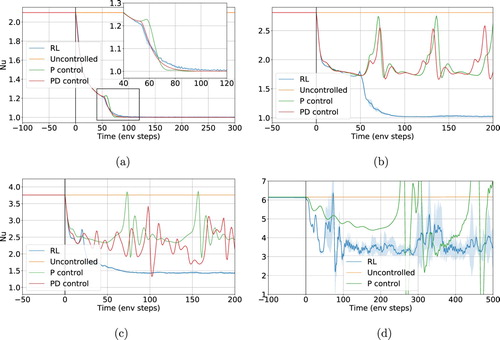
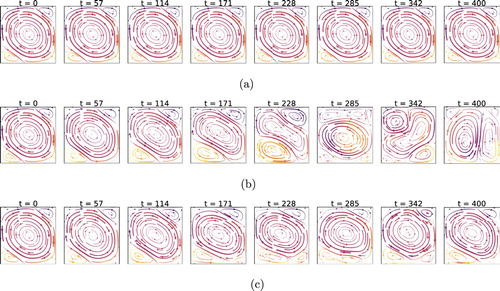
Figure 5. Instantaneous stream lines at different times, at $\mathrm{Ra}={10}^5$, comparison of cases without control (a), with linear control (b) and with RL-based control (c). Note that the time is given in units of $\mathrm{\Delta }t$ (i.e. control loop length, cf. Table A1. Note that the snapshots are taken at different instants). RL controls establish a flow regime like a ‘double cell mode’ which features a steady Nusselt number (see Figure 4c). This is in contrast with linear methods which rather produce a flow with fluctuating Nusselt. The double cell flow field has a significantly lower Nusselt number than the uncontrolled case, as heat transport to the top boundary can only happen via diffusion through the interface between the two cells. This ‘double cell’ control strategy is established by the RL control with any external supervision.

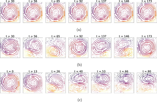
Figure 6. Instantaneous stream lines at $\mathrm{Ra}=3\cdot {10}^6$, comparison of cases without control (a), with linear control (b), and with RL-based control (c). We observe that the RL control still tries to enforce a ‘double cell’ flow, as in the lower Rayleigh case (Figure 5). The structure is, however, far less pronounced and convective effects are much stronger. This is likely due to the increased instability and chaoticity of the system, which increases the learning and controlling difficulty. Yet, we can observe a small alteration in the flow structure (cf. lower cell, larger in size than in uncontrolled conditions) which results in a slightly lower Nusselt number.

For the case $\mathrm{Ra}={10}^5$ (see Figure 5 c), the RL control steers and stabilises the system towards a configuration that resembles a double cell. This reduces convective effects by halving the effective Rayleigh number, $\mathrm{Ra}{}_{\mathrm{eff}}$, defined by the relation $\mathrm{Nu}{}_{\mathrm{uncontrolled}}(\mathrm{Ra}{}_{\mathrm{eff}})\approx \mathrm{Nu}{}_{\mathrm{RL}}(\mathrm{Ra})$. In particular, we can compute an effective Rayleigh number, $\mathrm{Ra}{}_{\mathrm{eff}}$, by observing that the double cell structure can be constructed as two vertically stacked Rayleigh–Bénard  systems with halved temperature difference and height (i.e. in formulas, $\mathrm{\Delta }{T}^{\prime }=\mathrm{\Delta }T/2$ and $H^{\prime }=H/2$). It thus results in an effective Rayleigh number satisfying (18) $\mathrm{Ra}{}_{\mathrm{eff}}=\frac{g\alpha \mathrm{\Delta }{T}^{\prime }{H}^{\prime 3}}{\nu \kappa }=\frac{1}{16}\frac{g\alpha \mathrm{\Delta }T{H}^3}{\nu \kappa }=\frac{1}{16}\mathrm{Ra},$(18) which is in line with the observed reduction in Nusselt.

At $\mathrm{Ra}=3\cdot {10}^6$, it appears that the RL control attempts, yet fails, to establish the ‘double cell’ configuration observed at lower $\mathrm{Ra}$ (cf. Figure 6 c). Likely, this is connected to the increased instability of the double cell configuration as Rayleigh increases.

These results were achieved with less than an hour of training time on an Nvidia V100 for the cases with low Rayleigh number ($\mathrm{Ra}\lesssim {10}^5$). However, at $\mathrm{Ra}\gtrsim {10}^6$ the optimization took up to 150 h of computing time (the majority of which is spent in simulations and the minority of which is spent in updating the policy). For further details on the training process of the RL controller, see Appendix 4.

4. Limits to learning and control

In this section, we discuss possible limits to the capability of learning automatic controls when aiming at suppressing convection. Our arguments are grounded on physics concepts and thus apply in general to control problems for non-linear/chaotic dynamics. Indeed, physical limitations might likely render some control problems unsolvable, either in absolute terms or by employing data-driven learning methods [44].

In Section 2, we showed that RL controls are capable of substantially outperforming linear methods in the presence of sufficient control complexity ($\mathrm{Ra}\gtrsim {10}^4$). It remains, however, unclear how far these controls are from optimality, especially at high Ra. Here we address the physics factors certainly hindering learning and controlling capabilities.

Having sufficient time and spatial resolution on the relevant state of the system is an obvious requirement to allow a successful control. Such resolution, however, is not defined in absolute terms, rather it connects to the typical scales of the system and, in case of a chaotic behaviour, with the Lyapunov time and associated length scale. In our case, at fixed Ra, learnability and controllability connect with the number and density of probes, with the time and space resolution of the control, but also with its ‘distance’ with respect to the bulk of the flow.

The system state is observed via a number of probes in fixed position (see Figure 1 b). For a typical (buoyant) velocity in the cell, $v_b$, there is a timescale associated with the delay with which a probe records a sudden change (e.g. creation/change of a plume) in the system. When this timescale becomes comparable or larger than the Lyapunov time, it appears hopeless for any control to learn and disentangle features from the probe readings. In other words, as $\mathrm{Ra}$ increases, we expect that a higher and higher number of probes becomes necessary (but not sufficient) in order to learn control policies.

Besides, our choice to control the system via the bottom plate temperature fluctuations entails another typical delay: the time taken to thermal adjustments to propagate inside the cell. In particular, in a cell at rest, this is the diffusion time, $t_D\sim H^2/\kappa \sim \mathrm{Ra}{}^{1/2}$. If the delay gets larger or comparable to the Lyapunov time, controlling the system becomes, again, likely impossible.

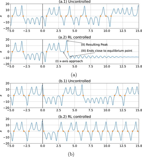
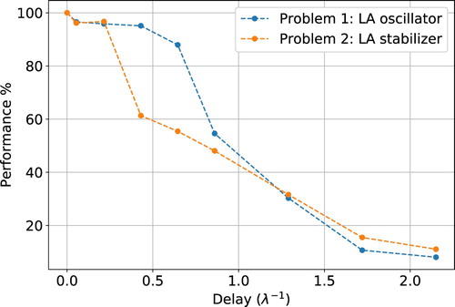
To illustrate this concept, we rely on a well-known low-dimensional model inspired by RBC: the Lorenz attractor. The attractor state is three-dimensional and its variables (usually denoted by x, y, z; see Appendix 5) represent the flow angular velocity, the horizontal temperature fluctuations and the vertical temperature fluctuations. We consider an RL control acting on the horizontal temperature fluctuations (y variable) that aims at either minimising or maximising the sign changes of the angular velocity (i.e. maximising or minimising the frequency of sign changes of the x variable). In other words, the control aims at keeping the flow rotation direction maximally consistent or, conversely, at magnifying the rate of velocity inversions. In this simplified context, we can easily quantify the effects of an artificial delay in the control on the overall control performance (Figure 7). Consistently with our previous observations, when the artificial delay approaches the Lyapunov time the control performance significantly degrades.

Figure 7. Performance loss due to an artificial delay imposed to an RL controller operating on the Lorenz attractor. The controller, operating on the y variable of the system (reduced model for the RBC horizontal temperature fluctuations) aims at either maximising (LA oscillator) or minimising (LA stabiliser) the number of sign changes of the x (in RBC terms the angular velocity of the flow). The delay, on the horizontal axis, is scaled on the Lyapunov time, ${\lambda }^{-1}$, of the system (with λ the largest Lyapunov exponent). In case of a delay in the control loop comparable in size to the Lyapunov time, the control performance diminishes significantly.

Notably, in our original 2D RBC control problem (Section 2), control limitations are not connected to delays in observability. In fact, as we consider coarser and coarser grids of probes, the control performance does not diminish significantly (cf. Figure 8; surprisingly, observations via only 4 allow similar control performance to what achieved employing 64 probes). This suggests that other mechanisms than insufficient probing determine the performance, most likely, the excessively long propagation time (in relation to the Lyapunov time) needed by the controlling actions to traverse the cell from the boundary to the bulk. This could be possibly lowered by considering different control and actuation strategies.

Figure 8. Average Nusselt number for an RL agent observing the Rayleigh–Bénard  environment at different probe density, all of which are lower than the baseline employed in Section 3. The grid sizes (i.e information) used to sample the state of the system at the Ra considered does not seem to play key role in limiting the final control performance of the RL agent.

5. Discussion

In this paper, we considered the issue of suppressing convective effects in a 2D Rayleigh–Bénard  cell, by applying small temperature fluctuations at the bottom plate. In our proof of concept comparison, limited to a square cell and fixed $\mathrm{Pr}$, we showed that controls based on RL are able to significantly outperform state-of-the-art linear approaches. Specifically, RL is capable of discovering controls stabilising the Rayleigh–Bénard  system up to a critical Rayleigh number that is approximately 3 times larger than achievable by state-of-the-art linear controllers and 30 times larger than in the uncontrolled case. Second, when the purely conductive state could not be achieved, the RL still produces control strategies capable of reducing convection, which are significantly better than linear algorithms. The RL control achieves this by inducing an unstable flow mode, similar to a stacked double-cell, yet not utilised in the context of RBC control.

Actually no guarantee exists on the optimality of the controls found by RL. Similarly it holds for the linear controls, which additionally need vast manual intervention for the identification of the parameters. However, as we showed numerically, theoretical bounds to controllability hold which are regulated by the chaotic nature of the system, i.e. by its Lyapunov exponents, in connection with the (space and time) resolution of the system observations as well as with the actuation capabilities. We quantified such theoretical bounds in terms of delays, in observability and/or in actuation: whenever these become comparable to the Lyapunov time, the control becomes impossible.

There is potential for the replication of this work in an actual experimental setting. However, training a controller only via experiments might take an excessively long time to converge. Recent developments in RL showed already the possibility of employing controllers partially trained on simulations (transfer learning [17]). Furthermore, the efficient design of experiments could be informed by further research in mapping the influence of the system parameters (e.g. aspect ratio, Pr number, locations and type of sensors) on the control and performance.

This would not only be a large step for the control of flows but also for RL where practical/industrial uses are still mostly lacking [14].

Disclosure statement

No potential conflict of interest was reported by the authors.

Appendices

Appendix 1. Rayleigh–Bénard simulation details

We simulate the Rayleigh–Bénard system via the lattice Boltzmann method (LBM) that we implement in a vectorised way on a GPU. We employ the following methods and schemes

• Velocity population: D2Q9 scheme, afterwards indicated by $f_i(\mathbf{x},t)$;

• Temperature population: D2Q4 scheme;

• Collision model: BGK collision operator [5,45];

• Forcing scheme: As seen in [5] most forcing schemes can be formulated as follows: (A1) $\begin{array}{rl}& f_i(\mathbf{x}+{\mathbf{e}}_i\mathrm{\Delta }t,t+\mathrm{\Delta }t)-f_i(\mathbf{x},t)=[{\mathrm{\Omega }}_i(\mathbf{x},t)+S_i(\mathbf{x},t)]\mathrm{\Delta }t\end{array}$(A1) (A2) $\begin{array}{rl}& {\mathbf{u}}^{\mathrm{eq}}=\frac{1}{\rho }\sum _i{f}_i{\mathbf{e}}_i+A\frac{\mathbf{F}\mathrm{\Delta }t}{\rho }\end{array}$(A2) with $S_i$ and A defined by scheme. We choose the scheme by He et al. [46] for its improved accuracy which reads (A3) $\begin{array}{rl}A& =\frac{1}{2}\end{array}$(A3) (A4) $\begin{array}{rl}{S}_i& =(1-\frac{\mathrm{\Delta }t}{2\tau })\frac{f_i^{\mathrm{eq}}}{\rho }\frac{{\mathbf{e}}_i-\mathbf{u}}{c_s^2}\mathbf{F}\end{array}$(A4)

• Boundary model: bounce-back rule enforcing no-slip boundary conditions [5].

To limit the training time, we implemented the LBM vectorising on the simulations. This enabled us to simulate multiple concurrent, fully independent, Rayleigh–Bénard  systems within a single process. This eliminates the overhead of having numerous individual processes running on a single GPU which would increase the CPU communication overhead. Validation of the simulation code has been done by comparison with analytical solutions of diffusion and flows resulting from forcing, and comparisons of Nusselt number at different Rayleigh numbers [47].

When an RL controller selects a temperature profile for the bottom boundary this is endured for number of LBM steps (this defines one environment step, or env step, with length $\mathrm{\Delta }t$ and is chosen to be approximately 1/20th of the convection time). The reason for these, so-called, sticky actions is that within one env step the system does not change significantly. Allowing quicker actions would not only be physically meaningless but also possibly detrimental to the performance (this is a known issue when training RL agents for games where actions need to be sustained to make an impact [41]). Furthermore, due to our need to investigate the transient behaviour, we set the episode length to 500 env steps (i.e. 500 actions can be taken before the evaluation stops). In this way, the transient is extinguished within the first 150 env steps. After each episode, the system is reset to a random, fully developed, convective RB state.

In dependence on the Rayleigh number (i.e. system size), it takes between millions and billions env steps to converge to a control strategy. To limit the computing time, we consider the smallest possible system that gives a good estimate for the uncontrolled Nusselt number (error within few percent).

In Table A1, we report the considered Rayleigh numbers and related system sizes.

Table A1. Rayleigh–Bénard  environments considered. For each Rayleigh number we report the LBM grid employed (size $N_X\times N_Y$), the uncontrolled Nusselt number measured from LBM simulations and a validation reference from the literature.

Ra	$N_X$ and $N_Y$	Length 1 env step (i.e. control loop length) (units: lbm steps)	Nu	Nu reference [47]
$1\cdot {10}^3$	20	16	1.000	1.000
$3\cdot {10}^3$	20	16	1.141
$1\cdot {10}^4$	20	30	2.090	2.15
$3\cdot {10}^4$	25	60	2.753
$1\cdot {10}^5$	30	60	3.847	3.91
$3\cdot {10}^5$	40	60	4.768
$1\cdot {10}^6$	100	60	6.136	6.3
$3\cdot {10}^6$	200	100	7.500
$1\cdot {10}^7$	350	180	10.900

Appendix 2. Control amplitude normalization

To limit the amplitude of the temperature fluctuations and ensure their zero-average (see Equations (7(7) $T_H=⟨T_B(x,t){⟩}_x,$(7) ), (9(9) ${\hat{T}}_B(x,t)|\le C\mathrm{\forall }x,t,$(9) )), we employ the following three normalization steps, indicated by $\mathcal{R}(\cdot )$ in the manuscript. Let ${\tilde{T}}_B(x,t)$ be the temperature fluctuation proposed by either the linear control or the RL-based control, we obtain ${\hat{T}}_B(x,t)$ as (A5) $\begin{array}{rl}& {\tilde{T}}_B^{\prime }(x,t)=\text{Clip}({\tilde{T}}_B(x,t),-C,C)\end{array}$(A5) (A6) $\begin{array}{rl}& {\tilde{T}}_B^{″}(x,t)={\tilde{T}}_B^{\prime }(x,t)-⟨{\tilde{T}}_B^{\prime }(x,t){⟩}_x\end{array}$(A6) (A7) $\begin{array}{rl}& {\hat{T}}_B(x,t)=\frac{{\tilde{T}}_B^{″}(x,t)}{\underset{x^{\prime }}{max}(1,|{\tilde{T}}_B^{″}(x,t)|/C)}.\end{array}$(A7) Note that the first operation is a clipping of the local temperature fluctuation between $\pm C$, which is necessary only for the linear control case.

Appendix 3. RL algorithm implementation and hyperparameters

In this appendix, we elaborate on our design choices about the implementation of RL for Rayleigh–Bénard  control.

• Discretization of the bottom boundary in 10 sections. A literature study [48,49] and preliminary experiments have shown that large/continuous action spaces are currently rather challenging for the convergence of RL methods. In our preliminary experiments, we observed that discretising $T_B$ in 20 sections was even less effective that in 10 sections, and that 5 sections were instead insufficient to get the desired performance.

• 3 layer multilayer perceptron (MLP) for state encoding. We considered this option over a convolutional neural network (CNN) applied on the entire lattice. The latter had significantly longer training times and lower final performance. Besides, we included in the state observed by the MLP the system readings in the D previous env steps, which is known to be beneficial for performance [41].

• PPO algorithm. We considered this option over value-based methods which were however more difficult to operate with due to the need of extensive hyperparameter tuning. Furthermore, we used the open source implementation of PPO included in the stable-baselines python library [50] (note: training PPO demands for a so-called auxiliary value function [40]. For that we employed a separate neural network having the same structure as the policy function).

A.1. Hyperparameters

We used the work by Burda et al. [41] as a starting point for our choice of the hyperparameters. We specifically considered two separate hyperparameter sets. (i) targeting final performance over training speed, used for $\mathrm{Ra}\le {10}^6$. (ii) targeting speed over final performance, used only on the highest Rayleigh number case ($\mathrm{Ra}>{10}^6$) and for the research on the probe density. Below one can see the PPO hyperparameters used (see [14,40] for further explanations).

• Number of concurrent environments: 512 (set 2: 128)

• Number of roll-out steps: 128

• Number of samples training samples: $512\cdot 128=65,536$ (set 2: $128\cdot 128=16,384$ )

• Entropy coefficient $c_s$: 0.01

• Learning rate α: $2.5\cdot {10}^{-4}$

• Discount factor γ: 0.99

• Number of mini-batches: 8 (set 2: 16)

• Number of epoch when optimising the surrogate: 4 (set 2: 32)

• Value function coefficient for the loss calculation: 0.5

• Factor for trade-off of bias vs. variance for Generalised Advantage Estimator Λ: 0.95

• PPO Clip-range: 0.2

Appendix 4. Training curves

We report in Figure 1 the learning curves for our RL control (performance vs. length of the training session). These curves provide information on the time necessary to converge to a strategy and thus are an indication of the difficulty and stability of the process. Note that a training step is equivalent to an environment step. We employ the terminology ‘training step’ for constancy with RL literature.

We stress that the PPO algorithm converged to similar controllers with analogous performance when repeating the training experiments (checked up to $\mathrm{Ra}={10}^6$).

Appendix 5. Implementation Lorentz Attractor Control

To illustrate our argument that a delay comparable to the Lyapunov time is detrimental to the control performance, we introduce two control problems defined on the Lorentz Attractor (LA). These LA control problems are defined considering the following equations: (A8) $\begin{array}{rl}& \dot{x}=\sigma (y-x),\end{array}$(A8) (A9) $\begin{array}{rl}& \dot{y}=x(\rho -z)-y+a,\end{array}$(A9) (A10) $\begin{array}{rl}& \dot{z}=xy-\beta z,\end{array}$(A10) (A11) $\begin{array}{rl}& \text{subject to}|a|\le 1\end{array}$(A11) with a being a relatively small controllable parameter, and $\sigma =10$, $\rho =28$ and $\beta =8/3$. The control loop and integration loop (via RK4) have the same time stepping $\mathrm{\Delta }t=0.05$. The two control problems are as follows:

1. ‘LA stabiliser’. We aim at minimising the frequency with which the flow direction changes (i.e. the frequency of x sign changes). Reward: $R_i=-1$ if $x_{i-1}{x}_i<0$ and zero otherwise;

2. ‘LA oscillator’. Similar to LA stabiliser but with inverse goal. Reward: $R_i=+1$ if $x_{i-1}{x}_i<0$ and zero otherwise.

We start the system in a random state around the attractor, the controller is an MLP network, and we use the PPO RL algorithm (similarly to our approach for the complete Rayleigh–Bénard  case). We furthermore limit the control to three states, $a=-1\vee 0\vee 1$, for training speed purposes.

Applying RL on these control problems with no delay results in the behaviours shown in Figure 2. The control develops complex strategies to maximise/minimise the frequency of sign changes of x.

Figure A1. Performance of RL during training (case of the Rayleigh–Bénard  system). We report the average Nusselt number and its fluctuations computed among a batch of 512 concurrent training environments. (a) ‘low’ Ra ($0\lesssim \mathrm{Ra}\lesssim 3\cdot {10}^4$) in which the control achieves $\mathrm{Nu}\approx 1$ in a stable way, (b)‘mid’ Ra ($3\cdot {10}^4\lesssim \mathrm{Ra}\lesssim 1\cdot {10}^6$) which still gives stable learning behaviour but converges to $\mathrm{Nu}>1$ and, lastly, (c) ‘high’ Ra ($1\cdot {10}^6\lesssim \mathrm{Ra}$) in which the higher chaoticity of the system makes a full stabilization impossible. (a) $\mathrm{Ra}=3\cdot {10}^4$ (‘low’). (b) $\mathrm{Ra}=3\cdot {10}^5$ (‘mid’) and (c) $\mathrm{Ra}=3\cdot {10}^6$ (‘high’).

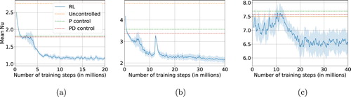
Figure A2. System trajectories with RL control, respectively aiming at minimising (a) and maximising (b) the number of x sign changes. In (a.1) and (b.1), we report two reference uncontrolled cases which differ only by the initialization state, $x(-5),y(-5),z(-5)$. Panel (a) shows that the RL agent is able to fully stabilise the system on an unstable equilibrium by using a complex strategy in three steps (I: controlling the system such that it approaches x, y, z = 0 which results in a peak (II) which after going through x = 0 ends close enough to an unstable equilibrium (III) such that the control is able to fully stabilise the system). Furthermore, Figure 2(a) shows that the RL agent is able to find and stabilise a unstable periodic orbits with a desired property of a high frequency of sign changes of x.

References

- Welty JR, Wicks CE, Rorrer G. Fundamentals of momentum, heat, and mass transfer. New York (New York): John Wiley & Sons; 2009.
- Chandrasekhar S. The instability of a layer of fluid heated below and subject to coriolis forces. Proc R Soc Lond Ser A Math Phys Sci. 1953;217(1130):306–327.
- Swaminathan A, Garrett SL, Poese ME, et al. Dynamic stabilization of the Rayleigh–Bénard instability by acceleration modulation. J Acoust Soc Amer. 2018;144(4):2334–2343. doi: 10.1121/1.5063820
- Müller G. Convection and inhomogeneities in crystal growth from the melt. In: Crystal growth from the melt. Springer; 1988. p. 1–136.
- Krüger T, Kusumaatmaja H, Kuzmin AV. The lattice Boltzmann method: principles and practice. Berlin: Springer International Publishing; 2017.
- Carbo RM, Smith RW, Poese ME. A computational model for the dynamic stabilization of Rayleigh–Bénard convection in a cubic cavity. J Acoust Soc Amer. 2014;135(2):654–668. doi: 10.1121/1.4861360
- Kelly R, Hu H. The effect of finite amplitude non-planar flow oscillations upon the onset of Rayleigh–Bénard convection. In: International Heat Transfer Conference Digital Library. Begel House Inc.; 1994.
- Davis SH. The stability of time-periodic flows. Ann Rev Fluid Mech. 1976;8(1):57–74. doi: 10.1146/annurev.fl.08.010176.000421
- Tang J, Bau HH. Stabilization of the no-motion state in the Rayleigh–Bénard problem. Proc Soc Lond Ser A Math Phys Sci. 1994;447(1931):587–607.
- Singer J, Bau HH. Active control of convection. Phys Fluids A Fluid Dyn. 1991;3(12):2859–2865. doi: 10.1063/1.857831
- Howle LE. Active control of Rayleigh–Bénard convection. Phys Fluids. 1997;9(7):1861–1863. doi: 10.1063/1.869335
- Or AC, Cortelezzi L, Speyer JL. Robust feedback control of Rayleigh–Bénard convection. J Fluid Mech. 2001;437:175–202. doi: 10.1017/S0022112001004256
- Remillieux MC, Zhao H, Bau HH. Suppression of Rayleigh–Bénard convection with proportional-derivative controller. Phys Fluids. 2007;19(1):017102. doi: 10.1063/1.2424490
- Sutton RS, Barto AG. Reinforcement learning: an introduction. Cambridge: MIT Press; 2018.
- Silver D, Schrittwieser J, Simonyan K, et al. Mastering the game of go without human knowledge. Nature. 2017;550(7676):354. doi: 10.1038/nature24270
- Silver D, Hubert T, Schrittwieser J, et al. A general reinforcement learning algorithm that masters chess, shogi, and go through self-play. Science. 2018;362(6419):1140–1144. doi: 10.1126/science.aar6404
- Andrychowicz OM, Baker B, Chociej M, et al. Learning dexterous in-hand manipulation. Inter J Robot Res. 2020;39(1):3–20. doi: 10.1177/0278364919887447
- Murphy KP. Machine learning: a probabilistic perspective. Cambridge: MIT Press; 2012.
- Hessel M, Modayil J, Van Hasselt H, et al. Rainbow: Combining improvements in deep reinforcement learning. In: Thirty-Second AAAI Conference on Artificial Intelligence; 2018.
- Carleo G, Cirac I, Cranmer K, et al. Machine learning and the physical sciences. Rev Modern Phys. 2019;91(4):045002. doi: 10.1103/RevModPhys.91.045002
- Brunton SL, Noack BR, Koumoutsakos P. Machine learning for fluid mechanics. Annu Rev Fluid Mech. 2020;52:477–508. doi: 10.1146/annurev-fluid-010719-060214
- Colabrese S, Gustavsson K, Celani A, et al. Smart inertial particles. Phys Rev Fluids. 2018;3(8):084301. doi: 10.1103/PhysRevFluids.3.084301
- Colabrese S, Gustavsson K, Celani A, et al. Flow navigation by smart microswimmers via reinforcement learning. Phys Rev Lett. 2017;118(15):158004. doi: 10.1103/PhysRevLett.118.158004
- Gustavsson K, Biferale L, Celani A, et al. Finding efficient swimming strategies in a three-dimensional chaotic flow by reinforcement learning. Euro Phys J E. 2017;40(12):110. doi: 10.1140/epje/i2017-11602-9
- Gazzola M, Tchieu AA, Alexeev D, et al. Learning to school in the presence of hydrodynamic interactions. J Fluid Mech. 2016;789:726–749. doi: 10.1017/jfm.2015.686
- Verma S, Novati G, Koumoutsakos P. Efficient collective swimming by harnessing vortices through deep reinforcement learning. Proc Natl Acad Sci. 2018;115(23):5849–5854. doi: 10.1073/pnas.1800923115
- Reddy G, Celani A, Sejnowski TJ, et al. Learning to soar in turbulent environments. Proc Nat Acad Sci. 2016;113(33):E4877–E4884. doi: 10.1073/pnas.1606075113
- Reddy G, Wong-Ng J, Celani A, et al. Glider soaring via reinforcement learning in the field. Nature. 2018;562(7726):236. doi: 10.1038/s41586-018-0533-0
- Biferale L, Bonaccorso F, Buzzicotti M, et al. Zermelo's problem: optimal point-to-point navigation in 2d turbulent flows using reinforcement learning. Chaos Interdisci J Nonlinear Sci. 2019;29(10):103138. doi: 10.1063/1.5120370
- Alageshan JK, Verma AK, Bec J, et al. Machine learning strategies for path-planning microswimmers in turbulent flows. Phys Rev E. 2020;101(4):043110. doi: 10.1103/PhysRevE.101.043110
- Rabault J, Kuchta M, Jensen A, et al. Artificial neural networks trained through deep reinforcement learning discover control strategies for active flow control. J Fluid Mech. 2019;865:281–302. doi: 10.1017/jfm.2019.62
- Muinos-Landin S, Ghazi-Zahedi K, Cichos F. Reinforcement learning of artificial microswimmers. arXiv preprint arXiv:180306425. 2018.
- Novati G, Mahadevan L, Koumoutsakos P. Controlled gliding and perching through deep-reinforcement-learning. Phys Rev Fluids. 2019;4(9):093902. doi: 10.1103/PhysRevFluids.4.093902
- Tsang ACH, Tong PW, Nallan S, et al. Self-learning how to swim at low Reynolds number. arXiv preprint arXiv:180807639. 2018.
- Rabault J, Kuhnle A. Accelerating deep reinforcement learning strategies of flow control through a multi-environment approach. Phys Fluids. 2019;31(9):094105. doi: 10.1063/1.5116415
- Cichos F, Gustavsson K, Mehlig B, et al. Machine learning for active matter. Nature Mach Intel. 2020;2(2):94–103. doi: 10.1038/s42256-020-0146-9
- Rabault J, Ren F, Zhang W, et al. Deep reinforcement learning in fluid mechanics: a promising method for both active flow control and shape optimization. J Hydrodyn. 2020;32:234–246. doi: 10.1007/s42241-020-0028-y
- Lorenz EN. Deterministic nonperiodic flow. J Atmos Sci. 1963;20(2):130–141. doi: 10.1175/1520-0469(1963)020<0130:DNF>2.0.CO;2
- Boyd S, Vandenberghe L. Convex optimization. Cambridge: Cambridge University Press; 2004.
- Schulman J, Wolski F, Dhariwal P, et al. Proximal policy optimization algorithms. arXiv preprint arXiv:170706347. 2017.
- Burda Y, Edwards H, Pathak D, et al. Large-scale study of curiosity-driven learning. arXiv preprint arXiv:180804355. 2018.
- Cybenko G. Approximation by superpositions of a sigmoidal function. Math Control Signals Syst. 1989;2(4):303–314. doi: 10.1007/BF02551274
- Rumelhart DE, Hinton GE, Williams RJ. Learning representations by back-propagating errors. Nature. 1986;323(6088):533–536. doi: 10.1038/323533a0
- Succi S, Coveney PV. Big data: the end of the scientific method? Philos Trans R Soc A. 2019;377(2142):20180145. doi: 10.1098/rsta.2018.0145
- Bhatnagar PL, Gross EP, Krook M. A model for collision processesin gases. I. Small amplitude processes in charged and neutral one-component systems. Phys Rev. 1954 May;94:511–525. doi: 10.1103/PhysRev.94.511
- He X, Shan X, Doolen GD. Discrete Boltzmann equation model for nonideal gases. Phys Rev E. 1998;57(1):R13. doi: 10.1103/PhysRevE.57.R13
- Ouertatani N, Cheikh NB, Beya BB, et al. Numerical simulation of two-dimensional Rayleigh–Bénard convection in an enclosure. Comp Rend Mécaniq. 2008;336(5):464–470. doi: 10.1016/j.crme.2008.02.004
- Lazaric A, Restelli M, Bonarini A. Reinforcement learning in continuous action spaces through sequential Monte Carlo methods. In: Advances in neural information processing systems; 2008. p. 833–840.
- Lee K, Kim SA, Choi J, et al. Deep reinforcement learning in continuous action spaces: a case study in the game of simulated curling. In: International Conference on Machine Learning; 2018. p. 2943–2952.
- Hill A, Raffin A, Ernestus M, et al. Stable baselines. Available from: https://github.com/hill-a/stable-baselines; 2018.