Build up of yield stress fluids via chaotic emulsification

Abstract

Stabilised dense emulsions display a rich phenomenology connecting microstructure and rheology. In this work, we study how an emulsion with a finite yield stress can be built via large-scale stirring. By gradually increasing the volume fraction of the dispersed minority phase, under the constant action of a stirring force, we are able to achieve a volume fraction close to $80\mathrm{\%}$. Despite the fact that our system is highly concentrated and not yet turbulent we observe a droplet size distribution consistent with the $-10/3$ scaling, often associated with inertial range droplets breakup. We report that the polydispersity of droplet sizes correlates with the dynamics of the emulsion formation process. Additionally, we quantify the visco-elastic properties of the dense emulsion finally obtained and we demonstrate the presence of a finite yield stress. The approach reported can pave the way to a quantitative understanding of the complex interplay between the dynamics of mesoscale constituents and the large-scale flow properties of yield stress fluids.

Keywords:

• Multiphase flows
• non-Newtonian fluids
• yield-stress fluids
• emulsification
• turbulence

1. Introduction

Emulsions, the dispersion of (at least) one liquid component into another in the form of droplets [1], are common to a vast number of products and applications, including food, cosmetics and oil industries [2–6]. The physics of emulsions presents many outstanding scientific challenges, connected with their rich phenomenology, which ranges from that of a non-Newtonian viscous fluid to an elastic solid [7] as the result of the strong coupling between the microscopic and macroscopic physics [8–11]. Despite the fact that much of this phenomenology seems universal and common to many soft-glassy materials (such as foams, gels, slurries, etc), the specific mechanical response of the emulsion strongly depends on its microstructure [9] and a fully quantitative theoretical understanding of the rheology-microstructure links is still lacking. Achieving certain rheological properties relies heavily on the capability to properly control how the emulsion is built. Nevertheless, much of the existing body of works (both experimental and numerical) focused rather on the effect of the physico-chemical properties of the liquids and surfactants, yielding a certain droplet elasticity or interfacial rheology [11–14]. In particular, in all the previous numerical studies of soft-glassy rheology, the system is assembled by simple juxtaposition of the elementary meso-constituents, with a given mean size and polydispersity, but according to an arbitrary distribution. Moreover, such distribution remains basically constant in time, for the soft particles that constitute the system cannot deform, break up or coalesce [15].

In this article, for the first time, starting with a fully phase-separated system, we describe, by means of high-resolution numerical simulations, the whole dynamics of the building up of a stabilised dense emulsion, of which we monitor the evolution (in both the dense and semi-diluted regimes) and measure the distribution of droplet sizes, during and after stirring. In the early phase of the forced regime, a power-law decay of the distribution with an exponent close to $-10/3$ is found, over a wide range of radii. Such scaling was found to be a rather robust and universal feature of stirred multiphase systems, from emulsions to the entrainment of air in the breaking of oceanic waves [16–19]. This $-10/3$ law was originally justified, for diluted systems, resorting to dimensional analysis [16]. Very recently, it was derived, more rigorously, by means of energetic arguments [20]. In both cases, though, a Kolmogorov-like turbulence phenomenology was invoked. Observing the same scaling in our jammed, non-turbulent, system challenges, then, the basic theoretical understanding of flow stirred emulsions, strongly pinpointing it as a still open problem. More generally we can accurately measure the time evolution of the droplet radii distribution function, and associated polydispersity, which we find to be an informative quantitative observable on the internal structure of the emulsions during the different phases of its dynamic evolution. We then rheologically characterise the emulsion, highlighting the presence of a finite yield stress and, finally, we discuss the possibility of probing the response of the system to changes in the control parameters.

2. Numerical setup and emulsification process

We consider binary mixtures, where the two constituent fluids have identical physical properties, namely the same density and viscosity. We perform direct numerical simulations in tri-periodic computational domains of size $L^3$ (with different resolutions L); our study employs a numerical model based on a Lattice Boltzmann method [21] implementing a nearest-neighbour lattice interaction of Shan-Chen type [22, 23] which endows the system with the nonideal character and gives rise to a surface tension, γ. A next-to-nearest neighbours interaction is also introduced, which promotes the emergence of a positive disjoining pressure within the thin liquid films between close-to-contact interfaces, thus inhibiting droplet coalescence [24, 25]. To give a hint of the quantities involved, the dimensionless maximum attained by the disjoining pressure (which occurs at a film thickness $h_0\approx 4$ lattice spacings) is ${\mathrm{\Pi }}_{\max }{h}_0/\gamma \approx 0.1$. This interaction provides, then, the required stabilising mechanism (mimicking the role of surfactants in standard emulsions and of nanoparticles in Pickering emulsions), that prevents the system from full phase separation and keeps the emulsion in its metastable state (the system experiences, in fact, a slow coarsening due to diffusion-driven coalescence events, but its time scale is too long to affect significantly the results of the present study [26]). The numerical model will not be discussed in further detail here, since it has been extensively validated against theoretical results and applied to the study on several physical problems, also in comparison with experiments, including rheology of confined foams [27, 28], plastic events and ‘avalanches’ in soft-glassy materials [26, 29–31], thermal convection in emulsions [32] and microfluidics [33, 34]. Numerical values of the relevant parameters used in the numerical simulations are reported in Table 1.

Table 1. Main parameters and relevant observables for all simulations, labelled by a ${\mathrm{RUN}}_{\mathrm{id}}$, presented in this paper: system size, L, (the grid spacing in all three directions is set to unity); energy injection rate, $E_{\mathrm{in}}=\overline{\mathbf{f}\cdot \mathbf{v}}$; root mean square velocity, $V_{\mathrm{rms}}=\sqrt{\overline{|\mathbf{v}{|}^2}}$; $T_L=L/V_{\mathrm{rms}}$ is the large-scale correlation time; ${\tau }_{\varphi }$ is the inverse injection rate; average number of droplets, $\overline{N_D}$; volume mean radius, $R_{30}=\sqrt[3]{\frac{3}{4\pi }⟨V_D⟩}$ ($V_D$ is the droplet volume); arithmetic mean radius, $R_{10}=⟨R⟩$; standard deviation of droplet radii, $R_{\sigma }$; capillary number, $Ca=\frac{\rho \nu V_{\mathrm{rms}}}{\sigma }$; Weber number, $We=\frac{\rho R_{10}{V}_{\mathrm{rms}}^2}{\sigma }$; Reynolds number as $Re=\frac{L{V}_{\mathrm{rms}}}{\nu }$.

${\mathrm{RUN}}_{\mathrm{id}}$	L	$E_{\mathrm{in}}$	$V_{\mathrm{rms}}$	$T_L$	${\tau }_{\varphi }/T_L$	$\overline{N_D}$	$R_{30}$	$R_{10}$	$R_{\sigma }$	Ca	We	Re
A	256	$7.196\cdot {10}^{-8}$	0.0115	22261	35.9	112.7	30.1	26.7	9.50	0.109	0.227	123.47
B	512	$6.294\cdot {10}^{-8}$	0.0178	28764	27.8	877.2	30.4	27.9	8.42	0.169	0.548	381.79
C	1024	$6.597\cdot {10}^{-8}$	0.0312	32821	24.4	5707.1	32.6	28.4	11.03	0.296	1.809	1339.27

Note: $\rho =1.36$ is the total fluid density, $\nu =c_s^2({\tau }_{\mathrm{LB}}-0.5)=1/6$ is the kinematic viscosity, equal for both pure fluids ($c_s=1/\sqrt{3}$ is the speed of sound and ${\tau }_{\mathrm{LB}}=1$ is the lattice Boltzmann relaxation time), and $\sigma =0.0238$ is the surface tension. The averages, $\overline{(\cdots )}$, are taken over time, in the interval $T_3$ (where the final concentration of the emulsion is achieved but the emulsion is still stirred), whereas the averages $⟨(\cdots )⟩$ are meant to taken over time and number of droplets.

A dense emulsion is characterised by a dispersed droplet phase with a volume fraction ϕ in the order or larger than the one corresponding to the random close packing of spheres ($\varphi \sim 64\mathrm{\%}$). Such high-volume fractions are achievable thanks to the deformability of droplets and to the stabilisation of interstitial liquid films (as discussed above).

Making a dense emulsion out of two volumes of fluids, $V_1$ and $V_2$, separated by a flat interface (in a container of volume $V=V_1+V_2$), is not an easy task. When a stirring force is applied the interface is broken and droplets are formed. However, it is not possible to attain a high droplet concentration, of the majority phase, simply by stirring. In fact, in this way, the phase-inverted state is energetically more favourable, whereby few droplets of the minority phase are dispersed in the continuous majority phase [35]. Therefore, we follow a procedure that closely resembles some recipes used to make mayonnaise at home. We start with a small volume fraction, $\varphi \sim 30\mathrm{\%}$ of ‘fluid one’ (say, e.g. oil), in a larger volume fraction, $\sim 70\mathrm{\%}$ of ‘fluid two’ (water). The two fluids are initially separated by a flat interface. At the beginning of the simulation a large-scale stirring is applied (as described in [36]), with an amplitude strong enough to break the initial interface and form droplets, but not too strong to destroy the emulsion (see simulation parameters in Table 1). Under these conditions, the forcing will deform (see Figure 1(a)) and break the flat interface in a multitude of droplets, creating a low-volume fraction emulsion of oil in water (see Figure 1(b–d)).

Figure 1. Graphical illustration of the emulsification process via large-scale stirring and slow injection of the dispersed phase. Snapshots of the interface (red/blue side corresponding to the continuous/dispersed phase) during stirring at various instants of time (given in units of the large-scale characteristic time $T_L=L/V_{\mathrm{rms}}$, where $V_{\mathrm{rms}}$ is computed once the injection process is terminated, i.e. at the maximum volume fraction; see also Figure 3 and caption therein). Both time and the volume fraction of the dispersed phase ϕ grow from (a)–(j). Panel (a): the slightly deformed initially flat interface is still clearly visible, no droplets have formed yet. Panels (b)–(d): the process of fragmentation of the initial interface, leading to the production of a large number of small droplets, can be appreciated (see e.g. panel (d)). Panels (e)–(j): ϕ further increases, droplets become smaller and the system becomes more and more densely packed. The simulation parameters are reported in Table 1 (run C). (a) $\varphi =30\mathrm{\%}$ $t=0.6T_L$ (b) $\varphi =31\mathrm{\%}$ $t=1.2T_L$ (c) $\varphi =32\mathrm{\%}$ $t=1.8T_L$ (d) $\varphi =33\mathrm{\%}$ $t=2.4T_L$ (e) $\varphi =35\mathrm{\%}$ $t=3T_L$ (f) $\varphi =42\mathrm{\%}$ $t=6T_L$ (g) $\varphi =50\mathrm{\%}$ $t=9T_L$ (h) $\varphi =60\mathrm{\%}$ $t=12T_L$ (i) $\varphi =70\mathrm{\%}$ $t=15T_L$ (j) $\varphi =77\mathrm{\%}$ $t=18T_L$.

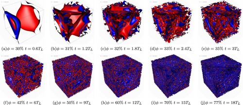
While the large-scale forcing is active, we slowly add oil (fluid one) and remove water (fluid two) in such a way to satisfy the constrain of total volume conservation. In Figure 1 the emulsions at times corresponding to $\varphi =30\mathrm{\%},31\mathrm{\%},32\mathrm{\%},33\mathrm{\%},35\mathrm{\%},42\mathrm{\%},50\mathrm{\%},60\mathrm{\%},70\mathrm{\%},77\mathrm{\%}$ are visualised. As it can be seen the process of adiabatically adding oil, while removing water, inflates the dispersed droplets already present in the emulsion until these break into smaller droplets due to hydrodynamics stresses induced by the large-scale stirring. In this way, it is possible to constantly produce new droplets and pack them to prepare an emulsion of high-volume fractions. All the snapshots in Figure 1 are collected along the stirred run (when the forcing is applied). When the forcing is switched off the emulsion relaxes to a resting state and droplets achieve a more isotropic shape.

In Figure 2 one can clearly appreciate the morphological difference between a high concentrated (left, corresponding to $\varphi =77\mathrm{\%}$) and a low concentrated emulsion (right, $\varphi =28\mathrm{\%}$): while at low-volume fraction the droplets maintain essentially their spherical shape, at high-volume fraction they are strongly deformed by the dense packing and squeeze the continuous phase into the typical network of foam-like structures. The droplet size in such a concentrated system is on average larger because, besides the high concentration of dispersed fluid, another effect comes into play. The mean size depends, in fact, on the competition between stirring and surface tension during the emulsification process. In particular, by Hinze's criterion [37], one expects the mean droplet size, R, to be determined by the Weber number, $We=\rho V_{\mathrm{rms}}^{2}R/\gamma$, being of order one, $We\sim 1$, which implies $R\sim V_{\mathrm{rms}}^{-2}\gamma$, i.e. the size decreases with the root mean square velocity. The latter, in turn, decreases with the effective viscosity (because the stirring force is kept constant) and hence with the dispersed phase volume fraction, which justifies, then, the larger droplet size in the more concentrated case.

Figure 2. Snapshot of the final interface field configuration from simulations with volume fraction $\varphi =77\mathrm{\%}$ (panel (a)) and $\varphi =28\mathrm{\%}$ (panel (b)). As it can be observed, at the largest volume fraction the droplets are highly deformed, while at lower volume fraction they preserve their equilibrium spherical shape and their average size is smaller. (a) ${512}^3$ – $\varphi =77\mathrm{\%}$ (b) ${512}^3$ – $\varphi =28\mathrm{\%}$.

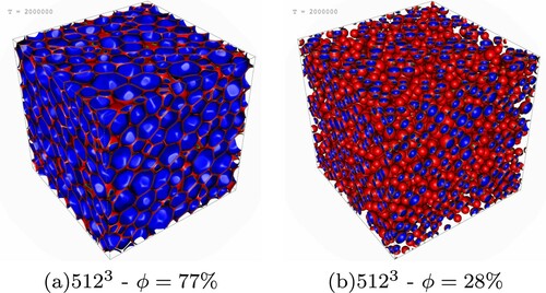
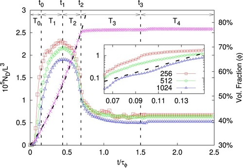
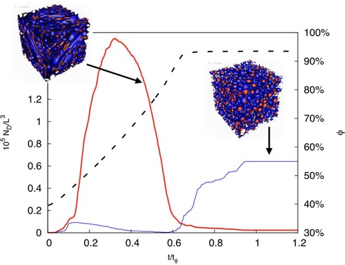
Figure 3. MAIN PANEL. Number density of droplets, $N_D/L^3$, as a function of time for different resolutions: L = 256 (red squares, $◻$), L = 512 (green circles, °) and L = 1024 (blue triangles, $\mathrm{△}$). The volume fraction of the dispersed phase, $\varphi (t)$, as a function of time is also reported on the $y2$-axis (magenta crosses, ×), together with an exponential fit in the injection phase $T_0+T_1+T_3$ (dashed line). The time is given in units of ${\tau }_{\varphi }$, the inverse injection rate (i.e. such that the total mass of dispersed phase fulfils $\dot{M}(t)={\tau }_{\varphi }^{-1}M(t)$). Further details on the parameter used in the simulations are provided in Table 1. INSET: Zoom on the first time window ($T_0$) in logarithmic scale on the y-axis to highlight the initial exponential increase of the number of droplets (the dashed line represents the exponential fit, drawn as a guide to the eye).

3. Droplet size distribution

The emulsion prepared with the procedure just described is characterised by a microstructure which is not assembled ad hoc, as customary in the large majority of numerical studies of soft-glassy rheology, but emerged, instead, naturally as the product of the flow dynamics and hydrodynamic stresses. It is therefore interesting to investigate the properties of the droplet size distribution (DSD), during the initial transient phase as well for the final resting dense emulsion. To our knowledge, this is the first time that this investigation is done during the emulsification process.

In this work, the strength of the large-scale stirring force is not enough to generate a fully developed turbulent flow, also due to the fact that the emulsion, at increasing the volume fraction of the dispersed phase, becomes more viscous. In Figure 3 we show the total number of droplets vs time (shown in units of the characteristic oil injection time, cfr. caption) for three different resolutions (with L = 256, 512, 1024). The magenta crosses show the time evolution of the volume fraction ϕ of the emulsion, see the right scale. At t = ∼0.6τ_Φ we stop increasing ϕ and keep it constant at $\varphi \sim 77\mathrm{\%}$. Looking at the total number of droplets, $N_D$, we can distinguish 5 different time windows in the system referred to as $T_i$, $i=0,\dots ,4$ and the corresponding ending times $t_k=\sum _{i=0}^k{T}_i$ (such that $T_k=t_k-t_{k-1}$). In the initial stage, $N_D$ grows quite rapidly during the time window $T_0$, it reaches a maximum in the time interval $[t_0,t_1]$ and then decreases in the interval $[t_1,t_2]$. At $t=t_2$ we stop increasing ϕ while retaining the large-scale forcing until a statistically steady state is reached; let us remark that simulations with a longer duration of this $T_3$ phase have been run, producing basically the same results in terms of droplets morphology and size distribution. Finally at $t=t_3$ we stop the large-scale forcing.

In Figure 4 we show the probability distribution $P_{\tau }(R)$ of finding a droplet with radius R during a time window τ. In panel (a), where $\tau \subset T_0$, a rather clear scaling $P_{\tau }(R)\sim R^{-10/3}$ is observed at relatively large R. This result is remarkable because it closely overlaps with what reported in the literature for breaking of oceanic waves and we believe it cannot be supported here by an argument based on turbulence inertial range scaling. It is also interesting to notice that the distribution decays much slower at large sizes than a compound Gamma function, as expected for the breakup of liquid jets or sheets [38]. This might be probably due to an important contribution coming from recoalescence events induced by the continuous stirring. Upon increasing the packing ratio, as shown in panels (b), for $\tau \subset T_1$, (c), for $\tau \subset T_2$, and in the early T3 phase, the shape of the distribution changes: the range where $P_{\tau }(R)\sim R^{-10/3}$ is reduced, the peak is shifted towards larger values of R and a new scaling behaviour $P_{\tau }(R)\sim R^{-6}$ is observed, with the change of slope occurring at $R\approx R_{30}$. Eventually, during the time windows $T_3$ and $T_4$, where the packing ratio is kept constant, there is no evidence of the scaling $-10/3$ (see panel (d)). It is interesting to observe that at the highest volume fraction, although for large values of R the DSDs in the forced ($T_3$) and unforced ($T_4$) cases are basically indistinguishable, a significant difference emerges at small sizes: under stirring, the presence of a second peak at $R\approx 0.15R_{30}$ can be detected, i.e. the $P_{T_3}(R)$ is bimodal. This secondary peak disappears when the forcing is switched off. We attribute this peak to the large number of breakup events for the high-volume fraction case. At further increasing the volume fraction of the dispersed case, or at increasing the intensity of the forcing, the emulsion rapidly breaks down via the so-called catastrophic phase inversion (see Figure 5). Figure 4 conveys the important message that the DSD of an emulsion (hence its polydispersity) relies crucially, and in a highly non-trivial way, on the preparation protocol, namely on the stirring and injection rate and their time duration. Consequently, our study suggests that, by leveraging the parameters that characterise these processes, one may envisage to control the emulsion microstructure and hence the rheology.

Figure 4. PDFs $P_{\tau }(R)$ (from the simulation C, see Table 1) of the effective droplet radii (i.e. for each droplet, the radius of the equivalent sphere is measured) given in units of the mean volume radius $R_{30}$, computed in four different time windows, τ. During the initial phase, $\tau \subset T_0$, the process of stirring-induced interface fragmentation dominates and the PDF displays a peak at $R\approx 0.15R_{30}$, followed by the typical slope $\sim R^{-10/3}$ (panel (a)). As the concentration of the dispersed phase increases, for $\tau \subset T_1$ a steeper decay, $\sim R^{-6}$, develops for large sizes, the change of slop occurring at $R\approx R_{30}$; in parallel, the peak is shifted towards higher R (panel (b)). Eventually, when the injection procedure is completed and the volume fraction of dispersed phase is $\approx 77\mathrm{\%}$, the peak merges with the bend at $R\approx R_{30}$ and a secondary peak emerges again at $R\approx 0.15R_{30}$, giving $P_{\tau }(R)$ (for $\tau \subset T_3$) a bimodal shape, evidence of the increasing presence of small droplets (panel (c)). This secondary maximum tends to vanish when the forcing is switched off (panel (d)).

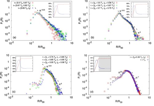
Figure 5. Time evolution of the number of droplets from a simulation of a system which eventually undergoes a catastrophic phase inversion: the red thick line indicates the droplets number for the ‘fluid 1’, $N_D^{(1)}$, namely the initially dispersed phase which gets progressively concentrated, whereas the blue thin line indicates $N_D^{(2)}$, the droplets number for ‘fluid 2’, the initially continuous phase; the black dashed line shows the growth of the volume fraction of ‘fluid 1’, ϕ. The two snapshots highlights the density field from configurations at two instants of time (indicated by the black arrows), respectively before and after the catastrophic phase inversion.

4. Emulsion rheology: yield stress and shear thinning

We move now to the rheological characterisation of the dense emulsions produced. To this aim, we take the emulsion configuration obtained at time $t_4$ and we apply a force of the form $\mathbf{F}=(F_x(y),0,0)$, where (1) $F_x(y)=F\sin \left(\frac{2\pi y}{L}\right),$(1) and monitor the response of the system at changing the amplitude F.

We use the forcing in Equation (1(1) $F_x(y)=F\sin \left(\frac{2\pi y}{L}\right),$(1) ) because it is compliant with the periodic boundary conditions used during the emulsification process. The shear stress induced by (1(1) $F_x(y)=F\sin \left(\frac{2\pi y}{L}\right),$(1) ) reads: (2) ${\sigma }_{xy}(y)\equiv \sigma (y)=\int F_x(y^{\prime })\mathrm{d}{y}^{\prime }=\frac{FL}{2\pi }\cos \left(\frac{2\pi y}{L}\right).$(2)

Following [39], we can define an effective stress as (3) ${\sigma }_{\mathrm{eff}}=⟨{\sigma }^2{⟩}^{1/2}=\left(\frac{L}{2\pi }\right)\frac{F}{\sqrt{2}}$(3) while the corresponding effective shear rate ${\dot{\gamma }}_{\mathrm{eff}}$ can be defined as (4) ${\dot{\gamma }}_{\mathrm{eff}}\equiv \frac{⟨\sigma (y)\dot{\gamma }(y)⟩}{⟨{\sigma }^2(y){⟩}^{1/2}},$(4) where the average is meant to be taken over y, i.e. $⟨(\dots )⟩=\frac{1}{L}{\int }_0^L(\dots )\mathrm{d}y$. 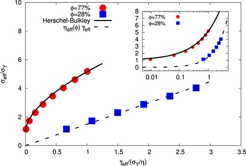From every simulation, with a certain forcing amplitude F, we are able to extract a couple $({\dot{\gamma }}_{\mathrm{eff}},{\sigma }_{\mathrm{eff}})$. The resulting flow curves are shown in Figure 6 for low- and high-volume fractions; in both cases, obviously, ${\sigma }_{\mathrm{eff}}$ grows with ${\dot{\gamma }}_{\mathrm{eff}}$, but while for $\varphi =28\mathrm{\%}$, as ${\dot{\gamma }}_{\mathrm{eff}}\to 0$, ${\sigma }_{\mathrm{eff}}$ vanishes, for $\varphi =77\mathrm{\%}$ the stress tends to a finite ‘yield’ value, ${\sigma }_Y$. Remarkably, for the high-volume fraction, the data could be fitted very well with a relation of the Herschel–Bulkley type, $\sigma ={\sigma }_Y+K{\dot{\gamma }}^{\beta }$, with ${\sigma }_Y=2.5\times {10}^{-5}$lbu, $K=0.02$lbu and $\beta =0.58$ (denoting a shear-thinning character). In contrast, the less concentrated system shows a Newtonian character, ${\sigma }_{\mathrm{eff}}={\eta }_{\mathrm{eff}}(\varphi ){\dot{\gamma }}_{\mathrm{eff}}$, though with an augmented (effective) viscosity that agrees with the Taylor expectation for diluted equiviscous emulsions, ${\eta }_{\mathrm{eff}}\approx \eta (1+(7/4)\varphi )$ (where $\eta =\rho \nu$ is the continuous phase dynamic viscosity) [40].

Figure 6. (Main panel) Flow curves for the emulsions with $\varphi =77\mathrm{\%}$ (red bullets) and $\varphi =28\mathrm{\%}$ (blue squares), showing effective shear stress, ${\sigma }_{\mathrm{eff}}$ (normalized with the yield stress ${\sigma }_Y$), vs effective shear rate, ${\dot{\gamma }}_{\mathrm{eff}}$ (normalized with the yield stress divided by the dynamics viscosity ${\sigma }_Y/\eta$), as defined in Equations (3(3) ${\sigma }_{\mathrm{eff}}=⟨{\sigma }^2{⟩}^{1/2}=\left(\frac{L}{2\pi }\right)\frac{F}{\sqrt{2}}$(3) )–(4(4) ${\dot{\gamma }}_{\mathrm{eff}}\equiv \frac{⟨\sigma (y)\dot{\gamma }(y)⟩}{⟨{\sigma }^2(y){⟩}^{1/2}},$(4) ). The solid line indicates a Herschel–Bulkley fit, $\sigma ={\sigma }_Y+K{\dot{\gamma }}^{\beta }$, with ${\sigma }_Y=2.5\times {10}^{-5}$ lbu, K = 0.02 lbu, $\beta =0.58$, whereas the dashed line represents the Newtonian relation $\sigma ={\eta }_{\mathrm{eff}}\dot{\gamma }$, with an effective viscosity compliant with the Taylor's prediction for equiviscous, low concentrated, emulsions, namely ${\eta }_{\mathrm{eff}}(\varphi )=\eta (1+(7/4)\varphi )$. (Inset) Same as in the main panel but in log-log scale.

Before concluding, let us underline, once more, that, in order to describe properly the rheology, it is crucial to have a realistic droplet size distribution. As a step further, then, we will show, in future works, how numerical simulations may help to correlate, quantitatively, the parameters controlling the emulsion preparation (e.g. stirring force amplitude, addition rate of the dispersed phase) to the those characterising the emulsion rheological properties (e.g. the yield stress).

5. Conclusions

We have demonstrated a numerical model and approach that allows to study the formation and dynamics of dense jammed emulsions with high space- and time-accuracy. The numerical method describes two immiscible fluids with surface tension and disjoining pressure, in order to stabilise droplets coalescence.

We focus on the production of a jammed emulsion by starting with a low-volume fraction, $\sim 30\mathrm{\%}$, of the dispersed phase and by continuous stirring to fragment droplets in a chaotic flow. Slowly increasing the dispersed phase we can achieve $\sim 80\mathrm{\%}$ volume fraction.

We measure the DSD and we show that soon after the breakup of the initially flat interface we can clearly detect a distribution of large droplet radii that seems in agreement with a $-10/3$ power-law scaling. At later times, during the process of increasing the volume fraction, the dynamics is dominated by droplets breakup event and the DSD displays two distinct scaling behaviours with much steeper exponents. At a very large volume fraction, $\approx 77\mathrm{\%}$, the DSD displays the emergence of a secondary peak around 1/10 of the average droplet radii. This peak is clearly associated with the dynamical flowing state, and ongoing fragmentation processes, as it disappears once the large-scale stirring is switched off.

While at the highest volume fraction achieved the system can still flow, for the forcing intensities that we employ, we demonstrate that this develops a finite yield stress. We show that such a state is stable under flow and that, switching off the stirring force, leads to a jammed state with finite yield stress. Increasing the forcing amplitude or the volume fraction of the dispersed phase leads to catastrophic phase inversion, a topic that will be studied in a forthcoming publication. This numerical approach offers unique perspectives to uncover the basic physics of dense emulsions, where the mesoscopic dynamics of droplets is extremely difficult to be studied via experimental techniques and paves the way to the use of simulations as a tool to guide a controlled emulsification, in order to obtain emulsions with targeted structural and rheological properties.

Disclosure statement

No potential conflict of interest was reported by the author(s).

Additional information

Funding

This work was supported by Partnership for Advanced Computing in Europe AISBL [grant numbers 2019204899, 2018184340].

References

- Tadros TF. Emulsion formation and stability. Wiley-VCH, Germany: Wiley; 2013.
- Gallegos C, Franco JM. Rheology of food, cosmetics and pharmaceuticals. Curr Opin Colloid Interface Sci. 1999;4(4):288–293.
- McClements DJ. Food emulsions: principles, practices and techniques. Boca Raton: CRC Press; 2015.
- Chang C, Nguyen QD, Rønningsen HP. Isothermal start-up of pipeline transporting waxy crude oil. J Non-Newton Fluid Mech. 1999;87(2–3):127–154.
- Egolf PW, Kauffeld M. From physical properties of ice slurries to industrial ice slurry applications. Int J Regrif. 2005;28(1):4–12.
- Coussot P. Rheometry of pastes, suspensions, and granular materials: applications in industry and environment. New York: Wiley; 2005.
- Larson RG. The structure and rheology of complex fluids. New York: Oxford University Press; 1998.
- Barnes HA. Rheology of emulsions – a review. Colloids Surf A. 1994;91:89–95.
- Pal R. Effect of droplet size on the rheology of emulsions. AIChE J. 1996;42(11):3181–3190.
- Mason TG. New fundamental concepts in emulsion rheology. Curr Opin Colloid Interface Sci. 1999;4(3):231–238.
- Derkach SR. Rheology of emulsions. Adv Colloid Interface Sci. 2009;151:1–23.
- Vankova N, Tcholakova S, Denkov ND, et al. Emulsification in turbulent flow 1. Mean and maximum drop diameters in inertial and viscous regimes. J Colloid Interface Sci. 2007;312:363–380.
- Vankova N, Tcholakova S, Denkov ND, et al. Emulsification in turbulent flow 2. Breakage rate constants. J Colloid Interface Sci. 2007;313:612–629.
- Vankova N, Tcholakova S, Denkov ND, et al. Emulsification in turbulent flow 3. Daughter drop-size distribution. J Colloid Interface Sci. 2007;310:570–589.
- Ikeda A, Berthier L, Sollich P. Unified study of glass and jamming rheology in soft particle systems. Phys Rev Lett. 2012;109:Article ID 018301.
- Garrett C, Li M, Farmer D. The connection between bubble size spectra and energy dissipation rates in the upper ocean. J Phys Oceanogr. 2000;30(9):2163–2171.
- Deane GB, Dale Stokes M. Scale dependence of bubble creation mechanisms in breaking waves. Nature. 2002;418(6900):839–844.
- Soligo G, Roccon A, Soldati A. Breakage, coalescence and size distribution of surfactant-laden droplets in turbulent flow. J Fluid Mech. 2019;881:244–282.
- Mukherjee S, Safdari A, Shardt O, et al. Droplet–turbulence interactions and quasi-equilibrium dynamics in turbulent emulsions. J Fluid Mech. 2019;878:221–276.
- Yu X, Hendrickson K, Yue DKP. Scale separation and dependence of entrainment bubble-size distribution in free-surface turbulence. J Fluid Mech. 2020;885.283.
- Succi S. The lattice Boltzmann equation: for fluid dynamics and beyond. Oxford: Clarendon Press; 2001.
- Shan X, Chen H. Lattice boltzmann model for simulating flows with multiple phases and components. Phys Rev E. 1993;47:1815–1819.
- Shan X, Chen H. Simulation of nonideal gases and liquid–gas phase transitions by the lattice boltzmann equation. Phys Rev E. 1994;49:2941–2948.
- Benzi R, Sbragaglia M, Succi S, et al. Mesoscopic lattice Boltzmann modeling of soft-glassy systems: theory and simulations. J Chem Phys. 2009;131(10):104903.
- Sbragaglia M, Benzi R, Bernaschi M, et al. The emergence of supramolecular forces from lattice kinetic models of non-ideal fluids: applications to the rheology of soft glassy materials. Soft Matter. 2012;8:10773–10782.
- Benzi R, Sbragaglia M, Scagliarini A, et al. Internal dynamics and activated processes in soft-glassy materials. Soft Matter. 2015;11:1271–1280.
- Dollet B, Scagliarini A, Sbragaglia M. Two-dimensional plastic flow of foams and emulsions in a channel: experiments and lattice Boltzmann simulations. J Fluid Mech. 2015;766:556–589.
- Scagliarini A, Dollet B, Sbragaglia M. Non-locality and viscous drag effects on the shear localisation in soft-glassy materials. Colloids Surf A. 2015;473:133–140.
- Benzi R, Pinaki K, Toschi F, et al. Earthquake statistics and plastic events in soft-glassy materials. Geophys J Int. 2016;207(3):1667–1674.
- Pelusi F, Benzi R, Sbragaglia M. Avalanche statistics during coarsening dynamics. Soft Matter. 2019;15:4518–4524.
- Kumar P, Korkolis E, Benzi R, et al. On interevent time distributions of avalanche dynamics. Sci Rep. 2020;10:3423.
- Pelusi F, Sbragaglia M, Benzi R, et al. Rayleigh-bénard convection of a model emulsion: anomalous heat-flux fluctuations and finite-size droplet effects. Soft Matter. 2021;17:3709–3721.
- Scagliarini A, Lulli M, Sbragaglia M, et al. Fluidisation and plastic activity in a model soft-glassy material flowing in micro-channels with rough walls. Europhys Lett. 2016;114(6):64003.
- Pelusi F, Sbragaglia M, Scagliarini A, et al. On the impact of controlled wall roughness shape on the flow of a soft material. Europhys Lett. 2019;127(3):34005.
- Vaessen GEJ, Stein HN. The applicability of catastrophe theory to emulsion phase inversion. J Colloid Interface Sci. 1995;176(2):378–387.
- Biferale L, Perlekar P, Sbragaglia M, et al. A lattice boltzmann method for turbulent emulsions. In J Phys: Conf Ser. 2011;318:21.
- Hinze JO. Fundamentals of the hydrodynamic mechanism of splitting in dispersion processes. AIChE J. 1955;1(3):289–295.
- Kooij S, Sijs R, Denn MM, et al. What determines the drop size in sprays? Phys Rev X. 2018;8:Article ID 031019.
- Benzi R, Bernaschi M, Sbragaglia M, et al. Herschel-Bulkley rheology from lattice kinetic theory of soft glassy materials. Europhys Lett. 2010;91:14003.
- Taylor GI. The viscosity of a fluid containing small drops of another fluid. Proc R Soc London, Ser B. 1932;138:41–48.