Experimental study of two side-by-side decaying grid turbulent fields at different mean velocities

Abstract

A Hot-wire anemometry experiment is conducted to investigate how two turbulent fields decaying with different mean velocities interact at their interface. A grid with different mesh sizes and solidities on either side of the grid centerline is used to generate two turbulent fields. It is found that the resulting turbulent shear layer created at the interface of the two fields evolves in a self-preserving manner. Further, the Taylor microscale Reynolds number, $R{e}_{\lambda }$ increases linearly while $\overline{u^2}$ and $\overline{q^2}$ become constants as the distance x downstream of the grids increases. Off the centerline one observes the classical decay of turbulence, e.g. $\overline{u^2}$ varies like $x^n$ (n is negative) and $R{e}_{\lambda }$ decreases. It is observed that the transport equation for $\overline{u^2}$ is dominated by the production and pressure-velocity correlation in the central region of the turbulent shear layer while production, dissipation, and turbulent diffusion of the transport equation for $\overline{q^2}$ dominate in the central part of the shear layer. The pressure-velocity correlation term for $\overline{q^2}$ is negligible on the centreline of the shear layer and important on the edges. The measurements of the scale-by-scale (SBS) energy terms on the shear layer centerline reveal that the energy transfer from large to small scales occurs in a non-trivial manner.

Keywords:

• Grid
• turbulent shear layer
• decay exponent
• energy budget

1. Introduction

The study of the mean shear effects on turbulence is of fundamental importance for understanding turbulent flows for example, wakes, jets, mixing layers, and wall turbulence, in general, where the mean velocity gradient plays a critical role in the dynamics of turbulence. The importance of the subject is reflected in the very large body of work available in the literature and is far too vast to be covered here. Despite this large number of research on the turbulent shear layer, there are still open questions that hinder the development not only of the fundamental but also the effective control strategies for achieving given outcomes, such as mixing enhancement or reduction, on a geophysical scale, how to make advance weather predictions as well as pollutant dispersion either in the atmosphere or ocean. One of these questions relate to the effect of mean shear on a scale-by-scale (SBS) basis, namely, how does the shear alter the energy distribution at all scale of motion, and can this effect be controlled?

To address the above question, one should try to isolate the effect of mean shear from other phenomena, such as anisotropy. For example, one possibility is to investigate turbulence behind the two side-by-side classical grids placed with different mesh sizes and solidities. Therefore, this study investigates the turbulent flows generated by a uniform flow when the fluid flows pass through the two side-by-side grids, and the interaction of the approximately homogeneous and isotropic flows on either side of the centreline. Consequently, the mean velocities on either side of the centreline are different, a mean velocity gradient develops downstream of the grid. This way a turbulent shear layer (hereafter, denoted TSL) is created in this study by using the grids. TSLs have already been subjected to many investigations (e.g. [1–8]). For example, [5] investigated the effects of the density ratio on the turbulent mixing layer in the TSL by using flow visualisation and found that the large-scale coherent structures were the fundamental features of the TSL. So far, it is noticed that only single-point statistics are investigated in TSLs. These statistics help in terms of gaining insights into the behaviour of turbulence. Therefore, they provided limited information on the dynamics of turbulence, especially when the emphasis is on small-scale turbulence. On the other hand, two-point statistics offer richer information, for example, they inform on the behaviour of turbulence at the various scales of motions (e.g. how the energy is distributed and exchanged among the scales). Unfortunately, there is no information currently available in the literature for the study of TSLs. As a result, it is important to discuss the scale-by-scale energy budget.

The scale-by-scale analysis in real space was first carried out by [9]. Starting with the Navier-Stokes equations, these authors developed an equation for the longitudinal velocity correlation function $f(r,t)$ (r is the space increment, and t is the time) for homogeneous and isotropic turbulence (HIT). This equation is commonly referred to as the Kàrmàn-Howarth equation and marked a milestone equation in the study of isotropic turbulence. However, the presence of an unknown quantity $h(r,t)$ called the triple velocity correlation function prevents one to solve this equation for $f(r,t)$. Therefore, this equation is nevertheless of great interest because it imposes constraints on the values of $f(r,t)$ and $h(r,t)$ that are compliant with the Navier-Stokes equations. Another attractive feature of the equation is that all of its terms can be relatively easily measured directly, thus allowing theoretical results to be tested. A further interesting feature of the Kármán-Howarth equation is that, in the limits $r\to 0$ and $r\to \mathrm{\infty }$, it reduces to the equations for the budgets enstrophy ($\overline{{\omega }^2}={\omega }_1^{{}^{\prime }2}+{\omega }_2^{{}^{\prime }2}+{\omega }_3^{{}^{\prime }2}$; ${\omega }_i$ are the fluctuating vorticity components and the prime represents the root mean square or rms) and the kinetic energy, respectively.

Kolmogorov [10] used the Kármán-Howarth equation to derive an equation, referred to as the Kolmogorov equation for the second-order structure function $\overline{(\delta u{)}^2}$ where $\delta u=\left(u\right(x,t)-u(x+r,t\left)\right)$ is the longitudinal velocity increment: (1) $-\overline{(\delta u{)}^3}+6\nu \frac{\mathrm{d}}{\mathrm{d}r}\overline{(\delta u{)}^2}=\frac{4}{5}\overline{ϵ}r$(1) where $\overline{ϵ}$ is the dissipation rate of the mean turbulent kinetic energy (the overbar represents time averaging). While, as for the Kármán-Howarth equation, (1(1) $-\overline{(\delta u{)}^3}+6\nu \frac{\mathrm{d}}{\mathrm{d}r}\overline{(\delta u{)}^2}=\frac{4}{5}\overline{ϵ}r$(1) ) is unclosed due to the presence of the term $\overline{(\delta u{)}^3}$, the equation is also of fundamental importance. In particular, it leads to the well-known four-fifths law in the inertial range, i.e. $-\overline{(\delta u{)}^3}=\left(4/5\right)\overline{ϵ}r$. When the Reynolds number is very large, Kolmogorov's equation can be interpreted as the balance at each scale of motions of the turbulent energy. On the left side of the equation, the first term (or inertial term) is the energy transfer arising from the interactions between the velocity fluctuations. The second term is the viscous term representing molecular diffusion. The right side of the equation is the energy transferred at scale r associated with $\overline{ϵ}$. Kolmogorov [10] derived Equation (1(1) $-\overline{(\delta u{)}^3}+6\nu \frac{\mathrm{d}}{\mathrm{d}r}\overline{(\delta u{)}^2}=\frac{4}{5}\overline{ϵ}r$(1) ) on the basis of local stationarity and locally isotropy turbulence. Accordingly, the equation can only accurately describe the dynamics of small-scale turbulence when it is free from any large-scale effects. The latter cannot be discounted in the presence of a mean shear flow, which is usually associated with a departure from homogeneity and isotropy on large scales.

However, a complete equation for $\overline{(\delta u{)}^2}$ (hereafter defined as the SBS energy budget equation) has been proposed by [11–16] which accounts for the large-scale inhomogeneities in the flow, although local homogeneity and isotropy is used in the derivation. This SBS energy budget equation was tested experimentally in grid turbulence (e.g. [14,17]), on the axis of a turbulent round jet (e.g. [18]), and the centreline of a turbulent channel flow (e.g. [19]) where the mean shear is either negligible or zero. It has also been extensively used to investigate the requirement of self-preservation in different turbulent flows (e.g. [20–25]).

This work, which is a natural continuation of a previous study [26], where two shearless decaying turbulent fields generated by a grid with two distinct mesh sizes (but the same solidity) on each side of the grid centerline, interacted in the absence of a mean shear. In that respect, it also represents a continuation of a pioneering work of [27] who also used a composite grid to generate a shearless turbulent mixing layer. The main aim of the present study is to assess how the addition of a mean shear can change the interaction of two decaying turbulent fields initially shearless. The focus will be on the impact of the mean shear on the energy transfer in the interaction region of the two decaying turbulent fields. The paper is organised as follows. In § 2, we present, the geometry of the novel composite grid which is used to generate the TSL. The measurement technique is also described in section § 2. In section § 3, we report on the main characteristics of the TSL; we discuss the individual terms in the transport equations for $\overline{u^2}$ and $\overline{q^2}=2k$ (u is the longitudinal velocity fluctuation component, and k is the turbulent kinetic energy) across the TSL. In § 4, SBS analysis of the TSL is carried out on the TSL centreline. Conclusions are presented in § 5.

2. Experimental setup and methodologies

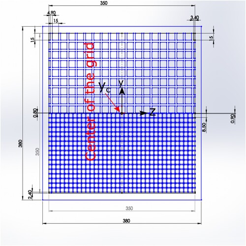
The measurements are carried out in an open circuit wind tunnel. The airflow is driven by a centrifugal blower, which is controlled by a variable-cycle (0–1500 rpm) power supply (Figure 1). To minimise vibration, the blower is supported by dampers and connected to the tunnel by a flexible joint. The wind tunnel has a working section with dimensions 2.4 m × 0.35 m × 0.35 m. More details of the wind tunnel are given in [22]. To generate two decaying turbulent fields evolving at different velocities a ‘composite’ grid is used: a perforated plate with square holes of different sizes on either side of the midsection of the grid (Figure 2). The mesh size is $M_L=19.9\mathrm{m}\mathrm{m}$ on the upper half and $M_S=10.2\mathrm{m}\mathrm{m}$ on the lower half (the subscripts S and L, hereafter refer to the small and large sections of the grid). The solidity σ for the lower and upper part of the grid is, respectively, ${\sigma }_S=30$% and ${\sigma }_L=43$%, $M_L/D_L=4.0$ and $M_S/D_S=5.0$) leading to $U_1=9.2\mathrm{m}/\mathrm{s}$ and $U_2=6.2\mathrm{m}/\mathrm{s}$ for the lower and upper free stream velocities. Here, $D_L$ and $D_s$ are the rod diameter in the upper and lower grids respectively. The use of these solidities and mesh sizes were shown to generate adequate decaying grid turbulence where homogeneity and isotropy are well approximated [24,28,29].

Figure 1. Geometrical configuration of the wind tunnel. The dimension of the working section is 2.4 m× 0.35 m×0.35 m.

Figure 2. Geometrical configuration of the grid, which generates the shear layer. The upper ($M_L=19.9\mathrm{m}\mathrm{m}$) and lower ($M_S=10.2\mathrm{m}\mathrm{m}$) parts of the grid have a different solidity (43% and 30%, respectively. All dimensions are in mm.)

Two types of hot-wire configurations were used and operated with an in-house constant temperature anemometer(CTA) at an overheat ratio of 1.8. Single hot-wire circuits were used to measure the $X-$components velocity (U) while X hot-wires were used to measure either the $X-$ and $Y-$ component velocities (U and V) or $X-$ and $Z-$ component velocities (U and W). The sensitive section of the hot-wire (diameter $d\approx 2.5\mu$m and length l = 200d) is etched from a coil of Wollaston (Pt-10%Rh) wire. The output signals from the CTA circuits are amplified, offset and low-pass filtered at a cut-off frequency ($f_c$) and a sampling frequency ($f_s$) at least equal to $2f_c$ with $2\times {10}^3\le f_c\le 4\times {10}^3$. Hereafter, the hot-wire signals are digitised into a PC using a ±10V and 16-bit AD converter. At each measurement point, the record duration is about $2min$ (∼ 120 second-and to ensure that all (one- and two-point) statistics have converged adequately. Using the same procedure as [30] for estimating the total uncertainty, the uncertainty is found to be about $\pm 2.6\mathrm{\%}$ for $u^{\prime }$ and $\pm 1.16\mathrm{\%}$ for $v^{\prime }$ (the prime represents rms). We use Taylor's hypothesis to convert temporal statistics to spatial statistics. This hypothesis is acceptable when the turbulence intensity $u^{\mathrm{\prime }}/U_c$ is small ( less than about 1 implies that $u^{\mathrm{\prime }}/U_c\ll 1$), which is the case here.

Figure 3 shows the distribution of $\overline{U}$ and $\overline{V}$, the mean velocity components along x and y, respectively, at a distance downstream of the composite $x/M_L=60$ (x is in the streamwise direction, and y is perpendicular to x as shown in Figure 2). The distributions of $\overline{U}$ indicate that two decaying turbulent fields each evolving at a different velocity are generated with a velocity gradient developing at their interface. 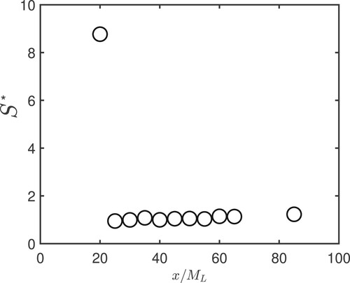The velocity component $\overline{V}$ is zero everywhere (as is $\overline{W}$, the spanwise velocity component, not shown here). Finally, we show (Figure 4) the distribution of the normalised shear parameter ($S^{\ast }=\left(dU/dy\right)u^{\prime 2}/\overline{ϵ}$) on the TSL centreline along the streamwise direction. This parameter is relatively large at $x/M_L=20$, indicating a strong shear in the region relatively close to the grid. However its value decreases sharply in the region $20\le x/M_L\le 25$ before remaining practically constant with increasing $x/M_L$.

Figure 3. Mean velocity in the longitudinal and lateral directions at $x/M_L=20$ and 60. Here $y_c$ is the center of the composite grid.

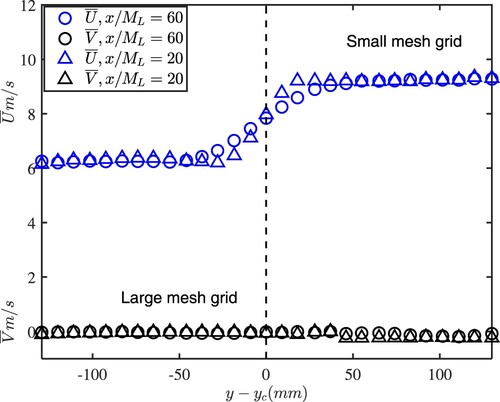
Figure 4. Distribution of the shear parameter $S^{\ast }$ on the TSL centerline.

3. Single-point measurements

3.1. Main characteristics of the TSL and its evaluation

To assess the decay of the TSL, we report the normalised mean velocity profiles in Figure 5 and the Reynolds stress distributions, $u^{\prime 2}$, $v^{\prime 2}$ and $\overline{uv}$ in Figure 6 for several distances downstream of the grid. The data are normalised with the scaling velocity $U_S=U_1-U_2$ (also called the shear velocity, where $U_1=9.3\mathrm{m}/\mathrm{s}$ and $U_2=6.3\mathrm{m}/\mathrm{s}$ are the largest and smallest velocities across the flow; see Figure 3 and the length scale $\delta =y_{0.95}-y_{0.1}$, where $y_{0.1}$ and $y_{0.95}$ correspond to the locations at which $\overline{U}=U_1+0.1U_S$ and $\overline{U}=U_2+0.95U_S$, respectively; we simply followed [2,7] for choosing $y_{0.1}$ and $y_{0.95}$.

Figure 5. Normalized mean velocity profiles at different downstream locations. The symbols $red▾$, $green◼$, $blue▴$, $\bullet$, $⧫$ are for $x/M_L=$ 20, 40, 60, 65 and 85, respectively.

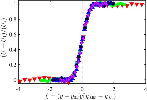
Figure 6. Normalized distributions of $u^{\mathrm{\prime }2}$ (a), $v^{\mathrm{\prime }2}$ (b) and $\overline{uv}$ (c) at different downstream locations. Symbols same as in Figure 5.

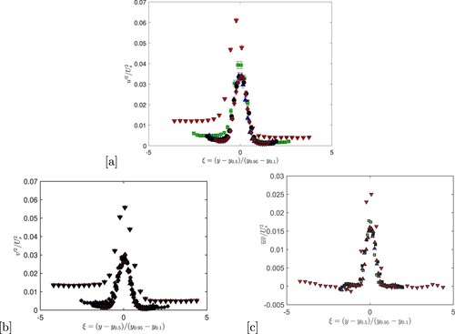
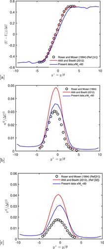
In Figure 7 we further compare these distributions with the direct numerical simulation (DNS) data of temporally [31] and spatially [32] evolving shear layers. There measurements profiles exhibit similar shapes to the DNS data, indicating that the interface at the two decaying turbulence field evolves like a classical TSL. The Reynolds shear stress $\overline{uv}$ is zero in both regions outside the shear layer where the turbulence is homogeneous. Also, the values of $u^{\prime 2}$ and $v^{\prime 2}$ in these regions reflect the two distinct levels the turbulence intensity: the larger values of $u^{\prime 2}$ and $v^{\prime 2}$ are, as expected, observed in the larger mesh side of the grid. The very good collapse of the distributions for $x/M_l\ge 40$, also observed in the DNS data of [31,32], indicates that the shear layer has reached a self-preserving state (notice the lack of collapse outside the TSL, where turbulence decay must follow that of classical grid turbulence). Interestingly, the mean velocity becomes self-similar at $x/M_L\ge 20$ compare to the Reynolds stresses, which is also observed in [32] who argued that the mean velocity profile alone may not be a reliable indicator of self-similarity.

Figure 7. Comparison with DNS data: Velocity U (a), $u^{\mathrm{\prime }2}$ (b), $v^{\mathrm{\prime }2}$ (c).

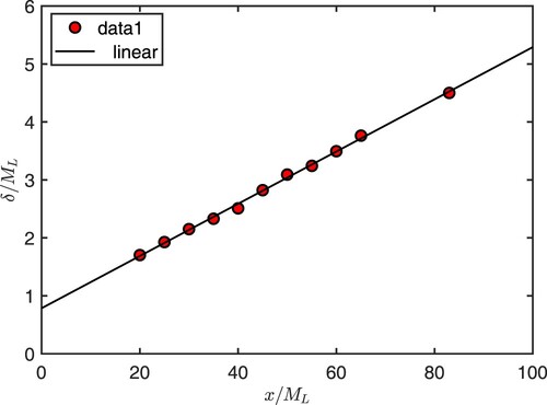
The self-similar behaviour of the TSL, at least from a mean velocity point of view, is also illustrated in Figure 8 which shows the variation of the TSL thickness with $x/M_L$. Self-similarity for the TSL requires that the characteristic length scale, δ, increases linearly with x [33], which is indeed well observed in Figure 8. The linear variation of δ is observed as early as $x/M_L=20$ corroborating the results of Figure 5.

Figure 8. Variation of the TSL thickness, δ, with the distance $x/M_L$. The straight line is used as a visual aid only.

To ascertain the difference between how turbulence decays within and outside the TSL, we report in Figure 9, the streamwise variations of $u^{\prime 2}$ on the centreline of the TSL and outside the TSL, both in the large mesh and small mesh sections. In these sections, the decay of $u^{\prime 2}$ follows the same law as that observed in classical grid turbulence, namely $u^{\prime 2}\sim x^n$ with n<−1; the difference in the decay exponent n between the two sections reflects the difference in mesh size and solidity. On the TSL centreline, $u^{\prime 2}$ first decreases before becoming practically constant for $x/M_L\ge 50$. Figure 10 shows the variation of Taylor microscale Reynolds nbmber $R{e}_{\lambda }$ (λ is the Taylor Microscale defined as $\sqrt{u^{\mathrm{\prime }2}/({\overline{\frac{\mathrm{d}u}{\mathrm{d}x})}}^2}$) on the TSL centreline: $R{e}_{\lambda }$ increases with increasing x. This behaviour is opposite to that observed outside the TSL (not shown here), where, as expected, $R{e}_{\lambda }$ decreases very slowly as x increases. Further, the magnitude of $R{e}_{\lambda }$ on the TSL centreline is larger than that outside the TSL where $R{e}_{\lambda }\simeq 60$ and 30 in the large mesh and small mesh sections, respectively. 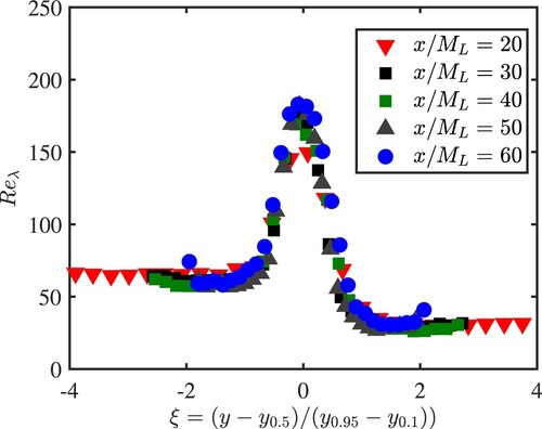Within the TSL, $R{e}_{\lambda }$ is maximum at the centreline and decreases to reach 60 and 30 outside the TSL as the distance from the centreline increases, as seen in Figure 11.

Figure 9. Decay of $u^{\prime 2}$ on the centreline (open circles) and outside (filled circles) of the TSL.

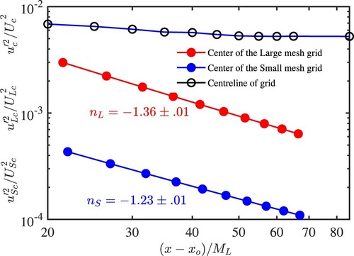
Figure 10. Variation of $R{e}_{\lambda }$ on the TSL centerline.

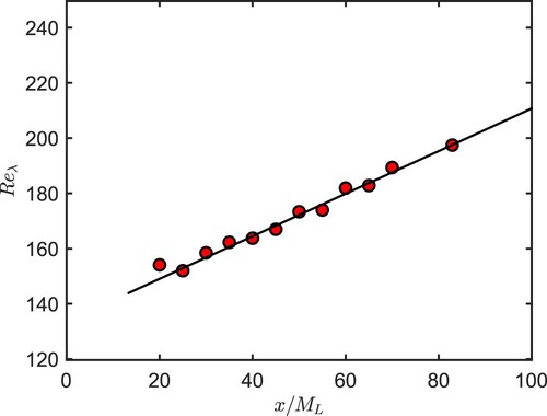
Figure 11. Variation of $R{e}_{\lambda }$ across the TSL at several $x/M_L$.

3.2. Transport equations for $\overline{u^2}$ and $\overline{q^2}$

The transport equation for $\overline{u^2}$ across the present shear layer reduces to (2) $\begin{array}{rl}\overline{U}\frac{\mathrm{\partial }\overline{u^2}}{\mathrm{\partial }x}+\frac{\mathrm{\partial }\overline{u^{2}v}}{\mathrm{\partial }y}& =-2\overline{uv}\frac{\mathrm{\partial }\overline{U}}{\mathrm{\partial }y}-2\overline{u\frac{\mathrm{\partial }\left(p/\rho \right)}{\mathrm{\partial }x}}\\ & -2\nu \left(\overline{\frac{\mathrm{\partial }u}{\mathrm{\partial }x}\frac{\mathrm{\partial }u}{\mathrm{\partial }x}}\right)+\nu \frac{{\mathrm{\partial }}^2\overline{u^2}}{\mathrm{\partial }{y}^2}\end{array}$(2) The left side term is the transport by convection. On the right side we have the production (1st term), the turbulent transport (or turbulent diffusion, 2nd term), the velocity-pressure gradient diffusion (3rd term), the destruction by viscosity Or dissipation (4th term) and viscous diffusion (5th terms). All the terms except the velocity-pressure gradient were measured; this latter term is obtained by difference. The velocity derivative $\mathrm{\partial }u/\mathrm{\partial }x$ is estimated by using Taylor's hypothesis (i.e., $\mathrm{\partial }x=\overline{U}\mathrm{\partial }t$). Figure 12 shows the terms of transport Equation (2(2) $\begin{array}{rl}\overline{U}\frac{\mathrm{\partial }\overline{u^2}}{\mathrm{\partial }x}+\frac{\mathrm{\partial }\overline{u^{2}v}}{\mathrm{\partial }y}& =-2\overline{uv}\frac{\mathrm{\partial }\overline{U}}{\mathrm{\partial }y}-2\overline{u\frac{\mathrm{\partial }\left(p/\rho \right)}{\mathrm{\partial }x}}\\ & -2\nu \left(\overline{\frac{\mathrm{\partial }u}{\mathrm{\partial }x}\frac{\mathrm{\partial }u}{\mathrm{\partial }x}}\right)+\nu \frac{{\mathrm{\partial }}^2\overline{u^2}}{\mathrm{\partial }{y}^2}\end{array}$(2) ) across the TSL at the distance $x/M_L=60$ downstream of the grid. The inset of the figure shows the DNS data of a temporally evolving turbulent mixing layer generated by two turbulent boundary layers on each side of a flat plate and merging behind the plate [31].

Since the last term on the right side of (2(2) $\begin{array}{rl}\overline{U}\frac{\mathrm{\partial }\overline{u^2}}{\mathrm{\partial }x}+\frac{\mathrm{\partial }\overline{u^{2}v}}{\mathrm{\partial }y}& =-2\overline{uv}\frac{\mathrm{\partial }\overline{U}}{\mathrm{\partial }y}-2\overline{u\frac{\mathrm{\partial }\left(p/\rho \right)}{\mathrm{\partial }x}}\\ & -2\nu \left(\overline{\frac{\mathrm{\partial }u}{\mathrm{\partial }x}\frac{\mathrm{\partial }u}{\mathrm{\partial }x}}\right)+\nu \frac{{\mathrm{\partial }}^2\overline{u^2}}{\mathrm{\partial }{y}^2}\end{array}$(2) ) is practically zero, it is not shown in the figure; this term is also found to be negligible at $x/M_L=20$, 30, 40 and 50. There is a good agreement, at least in terms of shape, between the various terms of the transport equation of $\overline{u^2}$ for the present data and that of DNS data of [31], lending confidence in the present measurements, which in turn instills confidence in the estimate of the velocity-pressure correlation term which was inferred indirectly by balancing Equation (2(2) $\begin{array}{rl}\overline{U}\frac{\mathrm{\partial }\overline{u^2}}{\mathrm{\partial }x}+\frac{\mathrm{\partial }\overline{u^{2}v}}{\mathrm{\partial }y}& =-2\overline{uv}\frac{\mathrm{\partial }\overline{U}}{\mathrm{\partial }y}-2\overline{u\frac{\mathrm{\partial }\left(p/\rho \right)}{\mathrm{\partial }x}}\\ & -2\nu \left(\overline{\frac{\mathrm{\partial }u}{\mathrm{\partial }x}\frac{\mathrm{\partial }u}{\mathrm{\partial }x}}\right)+\nu \frac{{\mathrm{\partial }}^2\overline{u^2}}{\mathrm{\partial }{y}^2}\end{array}$(2) ). Note that the difference in the normalisation leads to the difference in magnitudes between the measurements and the DNS data. The production and the pressure-velocity gradient terms dominate the budget across the TSL. The situation is somewhat different for the budget of $\overline{q^2}$ whose transport equation is written below (see Equation (3(3) $\begin{array}{rl}& \stackrel{\mathrm{a}\mathrm{d}\mathrm{v}\mathrm{e}\mathrm{c}\mathrm{t}\mathrm{i}\mathrm{o}\mathrm{n}}{\overbrace{\frac{1}{2}\overline{U}\frac{\mathrm{\partial }\overline{q^2}}{\mathrm{\partial }x}}}+\stackrel{\mathrm{p}\mathrm{r}\mathrm{o}\mathrm{d}\mathrm{u}\mathrm{c}\mathrm{t}\mathrm{i}\mathrm{o}\mathrm{n}}{\overbrace{\overline{uv}\frac{\mathrm{\partial }\overline{U}}{\mathrm{\partial }y}}}+\stackrel{\mathrm{t}\mathrm{u}\mathrm{r}\mathrm{b}\mathrm{u}\mathrm{l}\mathrm{e}\mathrm{n}\mathrm{t}\mathrm{d}\mathrm{i}\mathrm{f}\mathrm{f}\mathrm{u}\mathrm{s}\mathrm{i}\mathrm{o}\mathrm{n}}{\overbrace{\frac{1}{2}[\frac{\mathrm{\partial }\overline{q^{2}u}}{\mathrm{\partial }x}+\frac{\mathrm{\partial }\overline{v{q}^2}}{\mathrm{\partial }y}]}}\\ & +\stackrel{\mathrm{p}\mathrm{r}\mathrm{e}\mathrm{s}\mathrm{s}\mathrm{u}\mathrm{r}\mathrm{e}-\mathrm{v}\mathrm{e}\mathrm{l}\mathrm{o}\mathrm{c}\mathrm{i}\mathrm{t}\mathrm{y}\mathrm{c}\mathrm{o}\mathrm{r}\mathrm{r}\mathrm{e}\mathrm{l}\mathrm{a}\mathrm{t}\mathrm{i}\mathrm{o}\mathrm{n}}{\overbrace{\frac{1}{\rho }[\frac{\mathrm{\partial }\overline{pu}}{\mathrm{\partial }x}+\frac{\mathrm{\partial }\overline{pv}}{\mathrm{\partial }y}]}}+\stackrel{\mathrm{d}\mathrm{i}\mathrm{s}\mathrm{s}\mathrm{i}\mathrm{p}\mathrm{a}\mathrm{t}\mathrm{i}\mathrm{o}\mathrm{n}}{\overbrace{\overline{ϵ}}}=0\end{array}$(3) )). Note that since the viscous diffusion was found to be zero, we simply dropped it from the equation. Also, apart from the pressure-velocity term, which could not be measured, the dissipation $\overline{ϵ}$ poses a challenge as it involves twelve terms. However, if local isotropy (LI) is relatively well satisfied, then one can use $\overline{ϵ}\simeq {\overline{ϵ}}_{iso}$ where ${\overline{ϵ}}_{iso}$ is the isotropic value of the dissipation. For this reason, a test of LI is carried out by calculating the ratio $\alpha =\left(\mathrm{\partial }u/\mathrm{\partial }x{)}^2/\right(\mathrm{\partial }v/\mathrm{\partial }x{)}^2$ which is equal to 0.5 if LI is satisfied. It is found that for $x/M_L=60$ that $\alpha =0.5023,0.5109,0.5284,0.5061$ and 0.5225 at $(y-y_c)=-83,-37,0,37,83$ mm, respectively. This gives an average of approximately 0.5140, which is only 2$\mathrm{\%}$ higher than the isotropic value of 0.50. It is also observed that the value of α is 4$\mathrm{\%}$ larger on the centerline of the TSL; that value is 0.4253, 0.4675 and 0.4712 at $x/M_L=20$, 30, and 40 on the centerline. These results indicate that LI is relatively well satisfied across the TSL, at least at the location where the analysis is carried out, providing confidence in using ${\overline{ϵ}}_{iso}(=15\nu \overline{(\mathrm{d}u/\mathrm{d}x{)}^2})$ as a surrogate of $\overline{ϵ}$. We also estimated the difference between ${\overline{ϵ}}_{iso}$ and $\overline{ϵ}$ obtained using the spectral chart method (see, [34]) on the grid centerline and found to be only 7$\mathrm{\%}$, lending further support to the assumption of local isotropy. We now consider the transport equation for $\overline{q^2}$. (3) $\begin{array}{rl}& \stackrel{\mathrm{a}\mathrm{d}\mathrm{v}\mathrm{e}\mathrm{c}\mathrm{t}\mathrm{i}\mathrm{o}\mathrm{n}}{\overbrace{\frac{1}{2}\overline{U}\frac{\mathrm{\partial }\overline{q^2}}{\mathrm{\partial }x}}}+\stackrel{\mathrm{p}\mathrm{r}\mathrm{o}\mathrm{d}\mathrm{u}\mathrm{c}\mathrm{t}\mathrm{i}\mathrm{o}\mathrm{n}}{\overbrace{\overline{uv}\frac{\mathrm{\partial }\overline{U}}{\mathrm{\partial }y}}}+\stackrel{\mathrm{t}\mathrm{u}\mathrm{r}\mathrm{b}\mathrm{u}\mathrm{l}\mathrm{e}\mathrm{n}\mathrm{t}\mathrm{d}\mathrm{i}\mathrm{f}\mathrm{f}\mathrm{u}\mathrm{s}\mathrm{i}\mathrm{o}\mathrm{n}}{\overbrace{\frac{1}{2}[\frac{\mathrm{\partial }\overline{q^{2}u}}{\mathrm{\partial }x}+\frac{\mathrm{\partial }\overline{v{q}^2}}{\mathrm{\partial }y}]}}\\ & +\stackrel{\mathrm{p}\mathrm{r}\mathrm{e}\mathrm{s}\mathrm{s}\mathrm{u}\mathrm{r}\mathrm{e}-\mathrm{v}\mathrm{e}\mathrm{l}\mathrm{o}\mathrm{c}\mathrm{i}\mathrm{t}\mathrm{y}\mathrm{c}\mathrm{o}\mathrm{r}\mathrm{r}\mathrm{e}\mathrm{l}\mathrm{a}\mathrm{t}\mathrm{i}\mathrm{o}\mathrm{n}}{\overbrace{\frac{1}{\rho }[\frac{\mathrm{\partial }\overline{pu}}{\mathrm{\partial }x}+\frac{\mathrm{\partial }\overline{pv}}{\mathrm{\partial }y}]}}+\stackrel{\mathrm{d}\mathrm{i}\mathrm{s}\mathrm{s}\mathrm{i}\mathrm{p}\mathrm{a}\mathrm{t}\mathrm{i}\mathrm{o}\mathrm{n}}{\overbrace{\overline{ϵ}}}=0\end{array}$(3) Since it is found that the viscous term $\nu [\frac{{\mathrm{\partial }}^2{q}^2}{\mathrm{\partial }{x}^2}+\frac{{\mathrm{\partial }}^2{q}^2}{\mathrm{\partial }{y}^2}]$ is negligibly small it is dropped from the equation. The measured terms of (3(3) $\begin{array}{rl}& \stackrel{\mathrm{a}\mathrm{d}\mathrm{v}\mathrm{e}\mathrm{c}\mathrm{t}\mathrm{i}\mathrm{o}\mathrm{n}}{\overbrace{\frac{1}{2}\overline{U}\frac{\mathrm{\partial }\overline{q^2}}{\mathrm{\partial }x}}}+\stackrel{\mathrm{p}\mathrm{r}\mathrm{o}\mathrm{d}\mathrm{u}\mathrm{c}\mathrm{t}\mathrm{i}\mathrm{o}\mathrm{n}}{\overbrace{\overline{uv}\frac{\mathrm{\partial }\overline{U}}{\mathrm{\partial }y}}}+\stackrel{\mathrm{t}\mathrm{u}\mathrm{r}\mathrm{b}\mathrm{u}\mathrm{l}\mathrm{e}\mathrm{n}\mathrm{t}\mathrm{d}\mathrm{i}\mathrm{f}\mathrm{f}\mathrm{u}\mathrm{s}\mathrm{i}\mathrm{o}\mathrm{n}}{\overbrace{\frac{1}{2}[\frac{\mathrm{\partial }\overline{q^{2}u}}{\mathrm{\partial }x}+\frac{\mathrm{\partial }\overline{v{q}^2}}{\mathrm{\partial }y}]}}\\ & +\stackrel{\mathrm{p}\mathrm{r}\mathrm{e}\mathrm{s}\mathrm{s}\mathrm{u}\mathrm{r}\mathrm{e}-\mathrm{v}\mathrm{e}\mathrm{l}\mathrm{o}\mathrm{c}\mathrm{i}\mathrm{t}\mathrm{y}\mathrm{c}\mathrm{o}\mathrm{r}\mathrm{r}\mathrm{e}\mathrm{l}\mathrm{a}\mathrm{t}\mathrm{i}\mathrm{o}\mathrm{n}}{\overbrace{\frac{1}{\rho }[\frac{\mathrm{\partial }\overline{pu}}{\mathrm{\partial }x}+\frac{\mathrm{\partial }\overline{pv}}{\mathrm{\partial }y}]}}+\stackrel{\mathrm{d}\mathrm{i}\mathrm{s}\mathrm{s}\mathrm{i}\mathrm{p}\mathrm{a}\mathrm{t}\mathrm{i}\mathrm{o}\mathrm{n}}{\overbrace{\overline{ϵ}}}=0\end{array}$(3) ) across the TSL are reported in Figure 13 for $x/M_L=60$. Note that the molecular diffusion is not shown as it is practically zero everywhere. Using only single and X-wire probes poses a challenge for the measurement of the turbulent diffusion term since it requires the simultaneous measurements of the three velocity components in order to evaluate the correlation $\overline{q^{2}u}$ and $\overline{q^{2}v}$. 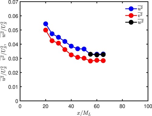Figure 14 shows the variation of the components $\overline{u^2}$, $\overline{v^2}$ and $\overline{w^2}$ along the centreline. Interestingly, we observe that $\overline{u^2}\simeq \overline{w^2}$. We use this result to write $\overline{q^2}=2\overline{u^2}+\overline{v^2}$ to calculate the correlations $\overline{q^{2}u}$ and $\overline{q^{2}v}$ across the TSL. We also use the approximation $\overline{q^2}=\overline{u^2}+2\overline{v^2}$ and found no significant change. We accordingly report the results using the former approximation of $\overline{q^2}$. Incidentally, Figure 14 reveals that $\overline{q^2}$ becomes practically constant for $x/M_L\ge 55$; in other words, the advection term in the budget of $\overline{q^2}$ should be negligibly small for $x/M_L\ge 55$, i.e. a close approximation to a homogeneous uniform shear flow.

Like the budget of $\overline{u^2}$, the measured distributions of the terms in (3(3) $\begin{array}{rl}& \stackrel{\mathrm{a}\mathrm{d}\mathrm{v}\mathrm{e}\mathrm{c}\mathrm{t}\mathrm{i}\mathrm{o}\mathrm{n}}{\overbrace{\frac{1}{2}\overline{U}\frac{\mathrm{\partial }\overline{q^2}}{\mathrm{\partial }x}}}+\stackrel{\mathrm{p}\mathrm{r}\mathrm{o}\mathrm{d}\mathrm{u}\mathrm{c}\mathrm{t}\mathrm{i}\mathrm{o}\mathrm{n}}{\overbrace{\overline{uv}\frac{\mathrm{\partial }\overline{U}}{\mathrm{\partial }y}}}+\stackrel{\mathrm{t}\mathrm{u}\mathrm{r}\mathrm{b}\mathrm{u}\mathrm{l}\mathrm{e}\mathrm{n}\mathrm{t}\mathrm{d}\mathrm{i}\mathrm{f}\mathrm{f}\mathrm{u}\mathrm{s}\mathrm{i}\mathrm{o}\mathrm{n}}{\overbrace{\frac{1}{2}[\frac{\mathrm{\partial }\overline{q^{2}u}}{\mathrm{\partial }x}+\frac{\mathrm{\partial }\overline{v{q}^2}}{\mathrm{\partial }y}]}}\\ & +\stackrel{\mathrm{p}\mathrm{r}\mathrm{e}\mathrm{s}\mathrm{s}\mathrm{u}\mathrm{r}\mathrm{e}-\mathrm{v}\mathrm{e}\mathrm{l}\mathrm{o}\mathrm{c}\mathrm{i}\mathrm{t}\mathrm{y}\mathrm{c}\mathrm{o}\mathrm{r}\mathrm{r}\mathrm{e}\mathrm{l}\mathrm{a}\mathrm{t}\mathrm{i}\mathrm{o}\mathrm{n}}{\overbrace{\frac{1}{\rho }[\frac{\mathrm{\partial }\overline{pu}}{\mathrm{\partial }x}+\frac{\mathrm{\partial }\overline{pv}}{\mathrm{\partial }y}]}}+\stackrel{\mathrm{d}\mathrm{i}\mathrm{s}\mathrm{s}\mathrm{i}\mathrm{p}\mathrm{a}\mathrm{t}\mathrm{i}\mathrm{o}\mathrm{n}}{\overbrace{\overline{ϵ}}}=0\end{array}$(3) ) are similar to those of [31], reported in the inset of the figure. Of particular interest is the comparison between the present distribution of the turbulent diffusion and that of [31]; the good agreement in the shape and location of the maxima and minimum is very good, giving some credence to the approximation $\overline{q^2}=2\overline{u^2}+\overline{v^2}$ for calculating the correlations $\overline{q^{2}u}$ and $\overline{q^{2}v}$ across the TSL. While the variation of the production, advection, dissipation, and turbulent diffusion across the TSL is similar to that observed in the $\overline{u^2}$-budget, the pressure-velocity term, here also inferred by balancing (3(3) $\begin{array}{rl}& \stackrel{\mathrm{a}\mathrm{d}\mathrm{v}\mathrm{e}\mathrm{c}\mathrm{t}\mathrm{i}\mathrm{o}\mathrm{n}}{\overbrace{\frac{1}{2}\overline{U}\frac{\mathrm{\partial }\overline{q^2}}{\mathrm{\partial }x}}}+\stackrel{\mathrm{p}\mathrm{r}\mathrm{o}\mathrm{d}\mathrm{u}\mathrm{c}\mathrm{t}\mathrm{i}\mathrm{o}\mathrm{n}}{\overbrace{\overline{uv}\frac{\mathrm{\partial }\overline{U}}{\mathrm{\partial }y}}}+\stackrel{\mathrm{t}\mathrm{u}\mathrm{r}\mathrm{b}\mathrm{u}\mathrm{l}\mathrm{e}\mathrm{n}\mathrm{t}\mathrm{d}\mathrm{i}\mathrm{f}\mathrm{f}\mathrm{u}\mathrm{s}\mathrm{i}\mathrm{o}\mathrm{n}}{\overbrace{\frac{1}{2}[\frac{\mathrm{\partial }\overline{q^{2}u}}{\mathrm{\partial }x}+\frac{\mathrm{\partial }\overline{v{q}^2}}{\mathrm{\partial }y}]}}\\ & +\stackrel{\mathrm{p}\mathrm{r}\mathrm{e}\mathrm{s}\mathrm{s}\mathrm{u}\mathrm{r}\mathrm{e}-\mathrm{v}\mathrm{e}\mathrm{l}\mathrm{o}\mathrm{c}\mathrm{i}\mathrm{t}\mathrm{y}\mathrm{c}\mathrm{o}\mathrm{r}\mathrm{r}\mathrm{e}\mathrm{l}\mathrm{a}\mathrm{t}\mathrm{i}\mathrm{o}\mathrm{n}}{\overbrace{\frac{1}{\rho }[\frac{\mathrm{\partial }\overline{pu}}{\mathrm{\partial }x}+\frac{\mathrm{\partial }\overline{pv}}{\mathrm{\partial }y}]}}+\stackrel{\mathrm{d}\mathrm{i}\mathrm{s}\mathrm{s}\mathrm{i}\mathrm{p}\mathrm{a}\mathrm{t}\mathrm{i}\mathrm{o}\mathrm{n}}{\overbrace{\overline{ϵ}}}=0\end{array}$(3) ), is significantly altered, like in the DNS data of [31]; it is practically zero on the centerline while being of maximum magnitude in the $\overline{u^2}$-budget. Rogers and Moser [31] showed that for the $\overline{u^2}$-budget equation, the pressure-velocity term involves both the ‘pressure strain rate correlation’ ($\overline{\frac{p}{\rho }(\frac{\mathrm{\partial }{u}_i}{\mathrm{\partial }{x}_j}+\frac{\mathrm{\partial }{u}_j}{\mathrm{\partial }{x}_i})}$) and the ‘pressure diffusion’ ($\frac{1}{\rho }({\delta }_{i2}\frac{\mathrm{\partial }\overline{p{u}_j}}{\mathrm{\partial }{x}_2}+{\delta }_{j2}\frac{\mathrm{\partial }\overline{p{u}_i}}{\mathrm{\partial }{x}_2})$), while it is entirely due to the latter in the $\overline{q^2}$-budget equation. Like the pressure-velocity term, the turbulent diffusion acts as a mechanism for redistributing the energy across the TSL; it extracts energy from the centreline and transfers it towards the edges. We also observe this mechanism in the DNS data of [31]. The role of the pressure-velocity term appears to be reversed, i.e. it transfers energy from the edges towards the centre of the TSL. As anticipated from Figure 14, the advection is negligible on the centreline; it is nevertheless maximum on the edges of the TSL.

Figure 12. Terms of the transport equation for $\overline{u^2}$ at $x/M_L=60$, normalised by $U_{Sc}^3/x^{-1}$. PVC stands for pressure velocity correlation. Inset: DNS data of [31] (with the permission of AIP Publishing), normalised by $U_{Sc}^3$ and ${\delta }_m$, theTSL momentum thickness.

Figure 13. Terms of the transport equation for $\overline{q^2}$ at $x/M_L=60$, normalised by $U_{Sc}^3/x^{-1}$. PVC stands for pressure velocity correlation. Inset: DNS data of [31], normalised by $U_{Sc}^3$ and ${\delta }_m$, the momentum thickness of the TSL. The inset figure is reproduced from Rogers, M. M., and Moser, R. D., ‘Direct simulation of a self-similar turbulent mixing layer,’ Phys. Fluids 6, 903–923 (1994), with the permission of AIP Publishing.

Figure 14. Variation of $\overline{u^2}$, $\overline{v^2}$ and $\overline{w^2}$ along the centreline.

The results presented above give an insight into how the production of energy associated with a mean shear is redistributed across the TSL. One interesting question is how such redistribution is felt at different scales of motion. To try and provide an answer to this question, we now turn our attention to the scale-by-scale energy budget. In this paper, we focus only on the centreline of the TSL, where production, dissipation, and diffusion are maximum.

4. Scale-by-scale energy budget on the TSL centreline

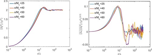
4.1. Second and third-order moments of $\delta u$ and $\delta q$

Before presenting the SBS energy budget of $\overline{\delta q^2}$ ($\equiv \overline{(\delta u{)}^2}+\overline{(\delta v{)}^2}+\overline{(\delta w{)}^2}$), we look at the distributions of $\overline{(\delta u{)}^2}$, $\overline{(\delta u{)}^3}$, $\overline{\left(\delta q^2\right)}$ and $\overline{\left(\delta u\right)\left(\delta q^2\right)}$. Figure 15 shows the distributions of $\overline{(\delta u{)}^2}/u^{\prime 2}$, and $\overline{(\delta u{)}^3}/u^{\prime 3}$ on the centreline. As expected, $\overline{(\delta u{)}^2}/u^{\prime 2}$ reaches the value of 2 at large separations. However, before reaching that value, the distribution displays a clear overshoot or hump when the separation falls in the range $10\le r/\lambda \le 30$. This hump is the ‘signature’ of large-scale coherent motions, which are also responsible for the undershoot, over the same range of separations, observed in the $\overline{(\delta u{)}^3}/u^{\prime 3}$ distributions. Similar observations can be made for $\overline{\left(\delta q^2\right)}/q^{\prime 2}$ and $\overline{\left(\delta u\right)\left(\delta q^2\right)}/(q^{\prime 2}{)}^{3/2}$ shown in Figure 16. We notice a reasonable level of the collapse of the distributions for the last two positions on the centreline, suggesting a possible onset of self-preservation, even though $R{e}_{\lambda }$ is increasing along the centreline (see Figure 10). Larger distances are needed before a definitive assessment regarding the collapse of the distributions can be given.

Figure 15. Distributions of $\overline{(\delta u{)}^2}$ and $\overline{(\delta u{)}^3}$ on the TSL centreline. The data are normalised by $u^{\prime }$ and λ.

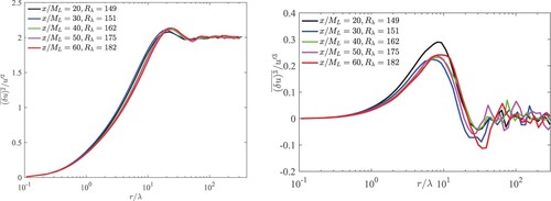
Figure 16. Distributions of $\overline{(\delta q{)}^2}$ and $\overline{(\delta q{)}^3}$ on the TSL centreline. The data are normalised by $q^{\mathrm{\prime }2}$ and λ.

We conclude this section by showing in Figure 17 the distributions of the skewness $S_{\overline{\delta u}}=\overline{(\delta u{)}^3}/(\overline{(\delta u{)}^2}{)}^{3/2}$ and the mixed skewness $S_{\overline{\delta q^2}}=\overline{\left(\delta u\right)\left(\delta q^2\right)}/\left[\right(\overline{(\delta u{)}^2}{)}^{1/2}\delta q^2]$. Quite remarkably, both appear to exhibit a plateau in the region $1\le r/\lambda \le 5$. However, considering the relatively short range of separations, it is not clear whether there is an actual plateau (which would imply the existence of an inertial rage) or an inflection point, which could be associated with the mean shear. Addressing this issue requires measurements at larger Reynolds numbers. This will allow a much larger separation between dissipative and large scales ranges.

Figure 17. Distributions of the skewness of $S_u$ on the centerline.

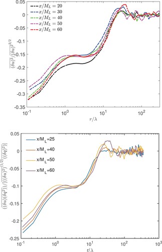
Like the distributions shown in Figures 15 and 16, the distributions for $S_{\overline{\delta u}}$ and $S_{\overline{\delta q^2}}$ appear to show some collapse, despite the scatter, in particular for small $r/\lambda$. The distribution of $S_{\delta u}$ for $x/M_L=20$ deviates significantly from the other distributions in the region $0.7\le r/\lambda \le 5$, reflecting the departure of the $\overline{(\delta u{)}^3}$- distribution from the other ones over practically the same range of scales (see Figure 15).

4.2. Scale-by-scale energy budget

We focus the SBS analysis on the grid centerline, although Figure 13 would suggest that the actual centerline of the TSL is slightly shifted toward the large mesh region with respect to the grid centerline by about $0.25M_L$. The budgets for $\overline{u^2}$ and $\overline{q^2}$ do not practically change between the two locations, suggesting that the SBS budget also remains practically unchanged. The grid centerline provides a better reference point than the TSL centerline for positioning the hot-wire probe. For convenience and since the TSL centerline and the grid centerline are close to each other, we simply assume they are the same line and do not hereafter differentiate between the two.

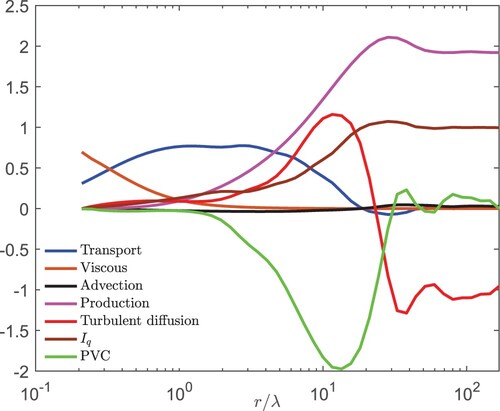
The SBS energy budget equation on the TSL centreline can be written as follows: (4) $\begin{array}{rl}& -\stackrel{\mathrm{t}\mathrm{r}\mathrm{a}\mathrm{n}\mathrm{s}\mathrm{p}\mathrm{o}\mathrm{r}\mathrm{t}}{\overbrace{\overline{\left(\delta q{)}^2\right(\delta u)}}}+\stackrel{\mathrm{v}\mathrm{i}\mathrm{s}\mathrm{c}\mathrm{o}\mathrm{u}\mathrm{s}}{\overbrace{2\nu \frac{\mathrm{d}}{\mathrm{d}r}\overline{(\delta q{)}^2}}}-\stackrel{\mathrm{a}\mathrm{d}\mathrm{v}\mathrm{e}\mathrm{c}\mathrm{t}\mathrm{i}\mathrm{o}\mathrm{n}}{\overbrace{\frac{\overline{U}}{r^2}{\int }_0^r{s}^2\frac{\mathrm{\partial }}{\mathrm{\partial }x}\overline{(\delta q{)}^2}\mathrm{d}s}}-\stackrel{\mathrm{p}\mathrm{r}\mathrm{o}\mathrm{d}\mathrm{u}\mathrm{c}\mathrm{t}\mathrm{i}\mathrm{o}\mathrm{n}}{\overbrace{\frac{2}{r^2}\frac{\mathrm{d}\overline{U}}{\mathrm{d}y}{\int }_0^r{s}^2\overline{\delta u\delta v}\mathrm{d}s}}\\ & -\stackrel{\mathrm{t}\mathrm{u}\mathrm{r}\mathrm{b}\mathrm{u}\mathrm{l}\mathrm{e}\mathrm{n}\mathrm{t}\mathrm{d}\mathrm{i}\mathrm{f}\mathrm{f}\mathrm{u}\mathrm{s}\mathrm{i}\mathrm{o}\mathrm{n}}{\overbrace{\frac{1}{r^2}{\int }_0^r{s}^2\frac{\mathrm{\partial }\overline{\left(v^{+}\right(\delta q{)}^2)}}{\mathrm{\partial }y}\mathrm{d}s}}+\stackrel{\mathrm{P}\mathrm{r}\mathrm{e}\mathrm{s}\mathrm{s}\mathrm{u}\mathrm{r}\mathrm{e}-\mathrm{v}\mathrm{e}\mathrm{l}\mathrm{o}\mathrm{c}\mathrm{i}\mathrm{t}\mathrm{y}}{\overbrace{PVC}}=\stackrel{\mathrm{d}\mathrm{i}\mathrm{s}\mathrm{s}\mathrm{i}\mathrm{p}\mathrm{a}\mathrm{t}\mathrm{i}\mathrm{o}\mathrm{n}}{\overbrace{\frac{4}{3}\overline{ϵ}r}}\end{array}$(4) The local isotropy assumption, which we found to be well satisfied across the TSL, was used. As for the single point budget equations, all terms except for the pressure velocity correlation term (PVC) were measured; the PVC term is obtained by balancing the equation. Figure 18 shows all the terms of (4(4) $\begin{array}{rl}& -\stackrel{\mathrm{t}\mathrm{r}\mathrm{a}\mathrm{n}\mathrm{s}\mathrm{p}\mathrm{o}\mathrm{r}\mathrm{t}}{\overbrace{\overline{\left(\delta q{)}^2\right(\delta u)}}}+\stackrel{\mathrm{v}\mathrm{i}\mathrm{s}\mathrm{c}\mathrm{o}\mathrm{u}\mathrm{s}}{\overbrace{2\nu \frac{\mathrm{d}}{\mathrm{d}r}\overline{(\delta q{)}^2}}}-\stackrel{\mathrm{a}\mathrm{d}\mathrm{v}\mathrm{e}\mathrm{c}\mathrm{t}\mathrm{i}\mathrm{o}\mathrm{n}}{\overbrace{\frac{\overline{U}}{r^2}{\int }_0^r{s}^2\frac{\mathrm{\partial }}{\mathrm{\partial }x}\overline{(\delta q{)}^2}\mathrm{d}s}}-\stackrel{\mathrm{p}\mathrm{r}\mathrm{o}\mathrm{d}\mathrm{u}\mathrm{c}\mathrm{t}\mathrm{i}\mathrm{o}\mathrm{n}}{\overbrace{\frac{2}{r^2}\frac{\mathrm{d}\overline{U}}{\mathrm{d}y}{\int }_0^r{s}^2\overline{\delta u\delta v}\mathrm{d}s}}\\ & -\stackrel{\mathrm{t}\mathrm{u}\mathrm{r}\mathrm{b}\mathrm{u}\mathrm{l}\mathrm{e}\mathrm{n}\mathrm{t}\mathrm{d}\mathrm{i}\mathrm{f}\mathrm{f}\mathrm{u}\mathrm{s}\mathrm{i}\mathrm{o}\mathrm{n}}{\overbrace{\frac{1}{r^2}{\int }_0^r{s}^2\frac{\mathrm{\partial }\overline{\left(v^{+}\right(\delta q{)}^2)}}{\mathrm{\partial }y}\mathrm{d}s}}+\stackrel{\mathrm{P}\mathrm{r}\mathrm{e}\mathrm{s}\mathrm{s}\mathrm{u}\mathrm{r}\mathrm{e}-\mathrm{v}\mathrm{e}\mathrm{l}\mathrm{o}\mathrm{c}\mathrm{i}\mathrm{t}\mathrm{y}}{\overbrace{PVC}}=\stackrel{\mathrm{d}\mathrm{i}\mathrm{s}\mathrm{s}\mathrm{i}\mathrm{p}\mathrm{a}\mathrm{t}\mathrm{i}\mathrm{o}\mathrm{n}}{\overbrace{\frac{4}{3}\overline{ϵ}r}}\end{array}$(4) ) on the centerline. We also report a term denoted $I_q$ which represents the total contribution of the non-homogeneous terms (advection, production, turbulent diffusion, and PVC) of (4(4) $\begin{array}{rl}& -\stackrel{\mathrm{t}\mathrm{r}\mathrm{a}\mathrm{n}\mathrm{s}\mathrm{p}\mathrm{o}\mathrm{r}\mathrm{t}}{\overbrace{\overline{\left(\delta q{)}^2\right(\delta u)}}}+\stackrel{\mathrm{v}\mathrm{i}\mathrm{s}\mathrm{c}\mathrm{o}\mathrm{u}\mathrm{s}}{\overbrace{2\nu \frac{\mathrm{d}}{\mathrm{d}r}\overline{(\delta q{)}^2}}}-\stackrel{\mathrm{a}\mathrm{d}\mathrm{v}\mathrm{e}\mathrm{c}\mathrm{t}\mathrm{i}\mathrm{o}\mathrm{n}}{\overbrace{\frac{\overline{U}}{r^2}{\int }_0^r{s}^2\frac{\mathrm{\partial }}{\mathrm{\partial }x}\overline{(\delta q{)}^2}\mathrm{d}s}}-\stackrel{\mathrm{p}\mathrm{r}\mathrm{o}\mathrm{d}\mathrm{u}\mathrm{c}\mathrm{t}\mathrm{i}\mathrm{o}\mathrm{n}}{\overbrace{\frac{2}{r^2}\frac{\mathrm{d}\overline{U}}{\mathrm{d}y}{\int }_0^r{s}^2\overline{\delta u\delta v}\mathrm{d}s}}\\ & -\stackrel{\mathrm{t}\mathrm{u}\mathrm{r}\mathrm{b}\mathrm{u}\mathrm{l}\mathrm{e}\mathrm{n}\mathrm{t}\mathrm{d}\mathrm{i}\mathrm{f}\mathrm{f}\mathrm{u}\mathrm{s}\mathrm{i}\mathrm{o}\mathrm{n}}{\overbrace{\frac{1}{r^2}{\int }_0^r{s}^2\frac{\mathrm{\partial }\overline{\left(v^{+}\right(\delta q{)}^2)}}{\mathrm{\partial }y}\mathrm{d}s}}+\stackrel{\mathrm{P}\mathrm{r}\mathrm{e}\mathrm{s}\mathrm{s}\mathrm{u}\mathrm{r}\mathrm{e}-\mathrm{v}\mathrm{e}\mathrm{l}\mathrm{o}\mathrm{c}\mathrm{i}\mathrm{t}\mathrm{y}}{\overbrace{PVC}}=\stackrel{\mathrm{d}\mathrm{i}\mathrm{s}\mathrm{s}\mathrm{i}\mathrm{p}\mathrm{a}\mathrm{t}\mathrm{i}\mathrm{o}\mathrm{n}}{\overbrace{\frac{4}{3}\overline{ϵ}r}}\end{array}$(4) ) and evaluated by subtracting the right side to the sum of the first and second terms on the left side.

Figure 18. Different terms of the SBS $\overline{\left(\delta q^2\right)}$-energy budget (Equation (4(4) $\begin{array}{rl}& -\stackrel{\mathrm{t}\mathrm{r}\mathrm{a}\mathrm{n}\mathrm{s}\mathrm{p}\mathrm{o}\mathrm{r}\mathrm{t}}{\overbrace{\overline{\left(\delta q{)}^2\right(\delta u)}}}+\stackrel{\mathrm{v}\mathrm{i}\mathrm{s}\mathrm{c}\mathrm{o}\mathrm{u}\mathrm{s}}{\overbrace{2\nu \frac{\mathrm{d}}{\mathrm{d}r}\overline{(\delta q{)}^2}}}-\stackrel{\mathrm{a}\mathrm{d}\mathrm{v}\mathrm{e}\mathrm{c}\mathrm{t}\mathrm{i}\mathrm{o}\mathrm{n}}{\overbrace{\frac{\overline{U}}{r^2}{\int }_0^r{s}^2\frac{\mathrm{\partial }}{\mathrm{\partial }x}\overline{(\delta q{)}^2}\mathrm{d}s}}-\stackrel{\mathrm{p}\mathrm{r}\mathrm{o}\mathrm{d}\mathrm{u}\mathrm{c}\mathrm{t}\mathrm{i}\mathrm{o}\mathrm{n}}{\overbrace{\frac{2}{r^2}\frac{\mathrm{d}\overline{U}}{\mathrm{d}y}{\int }_0^r{s}^2\overline{\delta u\delta v}\mathrm{d}s}}\\ & -\stackrel{\mathrm{t}\mathrm{u}\mathrm{r}\mathrm{b}\mathrm{u}\mathrm{l}\mathrm{e}\mathrm{n}\mathrm{t}\mathrm{d}\mathrm{i}\mathrm{f}\mathrm{f}\mathrm{u}\mathrm{s}\mathrm{i}\mathrm{o}\mathrm{n}}{\overbrace{\frac{1}{r^2}{\int }_0^r{s}^2\frac{\mathrm{\partial }\overline{\left(v^{+}\right(\delta q{)}^2)}}{\mathrm{\partial }y}\mathrm{d}s}}+\stackrel{\mathrm{P}\mathrm{r}\mathrm{e}\mathrm{s}\mathrm{s}\mathrm{u}\mathrm{r}\mathrm{e}-\mathrm{v}\mathrm{e}\mathrm{l}\mathrm{o}\mathrm{c}\mathrm{i}\mathrm{t}\mathrm{y}}{\overbrace{PVC}}=\stackrel{\mathrm{d}\mathrm{i}\mathrm{s}\mathrm{s}\mathrm{i}\mathrm{p}\mathrm{a}\mathrm{t}\mathrm{i}\mathrm{o}\mathrm{n}}{\overbrace{\frac{4}{3}\overline{ϵ}r}}\end{array}$(4) )) on the centerline at $x/M_L=60$. PVC stands for pressure velocity correlation. The data are normalised by (4/3)$\overline{ϵ}r$.

Before discussing the SBS budget, it is worthwhile verifying that at very large scales (4(4) $\begin{array}{rl}& -\stackrel{\mathrm{t}\mathrm{r}\mathrm{a}\mathrm{n}\mathrm{s}\mathrm{p}\mathrm{o}\mathrm{r}\mathrm{t}}{\overbrace{\overline{\left(\delta q{)}^2\right(\delta u)}}}+\stackrel{\mathrm{v}\mathrm{i}\mathrm{s}\mathrm{c}\mathrm{o}\mathrm{u}\mathrm{s}}{\overbrace{2\nu \frac{\mathrm{d}}{\mathrm{d}r}\overline{(\delta q{)}^2}}}-\stackrel{\mathrm{a}\mathrm{d}\mathrm{v}\mathrm{e}\mathrm{c}\mathrm{t}\mathrm{i}\mathrm{o}\mathrm{n}}{\overbrace{\frac{\overline{U}}{r^2}{\int }_0^r{s}^2\frac{\mathrm{\partial }}{\mathrm{\partial }x}\overline{(\delta q{)}^2}\mathrm{d}s}}-\stackrel{\mathrm{p}\mathrm{r}\mathrm{o}\mathrm{d}\mathrm{u}\mathrm{c}\mathrm{t}\mathrm{i}\mathrm{o}\mathrm{n}}{\overbrace{\frac{2}{r^2}\frac{\mathrm{d}\overline{U}}{\mathrm{d}y}{\int }_0^r{s}^2\overline{\delta u\delta v}\mathrm{d}s}}\\ & -\stackrel{\mathrm{t}\mathrm{u}\mathrm{r}\mathrm{b}\mathrm{u}\mathrm{l}\mathrm{e}\mathrm{n}\mathrm{t}\mathrm{d}\mathrm{i}\mathrm{f}\mathrm{f}\mathrm{u}\mathrm{s}\mathrm{i}\mathrm{o}\mathrm{n}}{\overbrace{\frac{1}{r^2}{\int }_0^r{s}^2\frac{\mathrm{\partial }\overline{\left(v^{+}\right(\delta q{)}^2)}}{\mathrm{\partial }y}\mathrm{d}s}}+\stackrel{\mathrm{P}\mathrm{r}\mathrm{e}\mathrm{s}\mathrm{s}\mathrm{u}\mathrm{r}\mathrm{e}-\mathrm{v}\mathrm{e}\mathrm{l}\mathrm{o}\mathrm{c}\mathrm{i}\mathrm{t}\mathrm{y}}{\overbrace{PVC}}=\stackrel{\mathrm{d}\mathrm{i}\mathrm{s}\mathrm{s}\mathrm{i}\mathrm{p}\mathrm{a}\mathrm{t}\mathrm{i}\mathrm{o}\mathrm{n}}{\overbrace{\frac{4}{3}\overline{ϵ}r}}\end{array}$(4) ) reduces to the single point energy budget (3(3) $\begin{array}{rl}& \stackrel{\mathrm{a}\mathrm{d}\mathrm{v}\mathrm{e}\mathrm{c}\mathrm{t}\mathrm{i}\mathrm{o}\mathrm{n}}{\overbrace{\frac{1}{2}\overline{U}\frac{\mathrm{\partial }\overline{q^2}}{\mathrm{\partial }x}}}+\stackrel{\mathrm{p}\mathrm{r}\mathrm{o}\mathrm{d}\mathrm{u}\mathrm{c}\mathrm{t}\mathrm{i}\mathrm{o}\mathrm{n}}{\overbrace{\overline{uv}\frac{\mathrm{\partial }\overline{U}}{\mathrm{\partial }y}}}+\stackrel{\mathrm{t}\mathrm{u}\mathrm{r}\mathrm{b}\mathrm{u}\mathrm{l}\mathrm{e}\mathrm{n}\mathrm{t}\mathrm{d}\mathrm{i}\mathrm{f}\mathrm{f}\mathrm{u}\mathrm{s}\mathrm{i}\mathrm{o}\mathrm{n}}{\overbrace{\frac{1}{2}[\frac{\mathrm{\partial }\overline{q^{2}u}}{\mathrm{\partial }x}+\frac{\mathrm{\partial }\overline{v{q}^2}}{\mathrm{\partial }y}]}}\\ & +\stackrel{\mathrm{p}\mathrm{r}\mathrm{e}\mathrm{s}\mathrm{s}\mathrm{u}\mathrm{r}\mathrm{e}-\mathrm{v}\mathrm{e}\mathrm{l}\mathrm{o}\mathrm{c}\mathrm{i}\mathrm{t}\mathrm{y}\mathrm{c}\mathrm{o}\mathrm{r}\mathrm{r}\mathrm{e}\mathrm{l}\mathrm{a}\mathrm{t}\mathrm{i}\mathrm{o}\mathrm{n}}{\overbrace{\frac{1}{\rho }[\frac{\mathrm{\partial }\overline{pu}}{\mathrm{\partial }x}+\frac{\mathrm{\partial }\overline{pv}}{\mathrm{\partial }y}]}}+\stackrel{\mathrm{d}\mathrm{i}\mathrm{s}\mathrm{s}\mathrm{i}\mathrm{p}\mathrm{a}\mathrm{t}\mathrm{i}\mathrm{o}\mathrm{n}}{\overbrace{\overline{ϵ}}}=0\end{array}$(3) ), as it should. We thus report in Table 1 the terms of (3(3) $\begin{array}{rl}& \stackrel{\mathrm{a}\mathrm{d}\mathrm{v}\mathrm{e}\mathrm{c}\mathrm{t}\mathrm{i}\mathrm{o}\mathrm{n}}{\overbrace{\frac{1}{2}\overline{U}\frac{\mathrm{\partial }\overline{q^2}}{\mathrm{\partial }x}}}+\stackrel{\mathrm{p}\mathrm{r}\mathrm{o}\mathrm{d}\mathrm{u}\mathrm{c}\mathrm{t}\mathrm{i}\mathrm{o}\mathrm{n}}{\overbrace{\overline{uv}\frac{\mathrm{\partial }\overline{U}}{\mathrm{\partial }y}}}+\stackrel{\mathrm{t}\mathrm{u}\mathrm{r}\mathrm{b}\mathrm{u}\mathrm{l}\mathrm{e}\mathrm{n}\mathrm{t}\mathrm{d}\mathrm{i}\mathrm{f}\mathrm{f}\mathrm{u}\mathrm{s}\mathrm{i}\mathrm{o}\mathrm{n}}{\overbrace{\frac{1}{2}[\frac{\mathrm{\partial }\overline{q^{2}u}}{\mathrm{\partial }x}+\frac{\mathrm{\partial }\overline{v{q}^2}}{\mathrm{\partial }y}]}}\\ & +\stackrel{\mathrm{p}\mathrm{r}\mathrm{e}\mathrm{s}\mathrm{s}\mathrm{u}\mathrm{r}\mathrm{e}-\mathrm{v}\mathrm{e}\mathrm{l}\mathrm{o}\mathrm{c}\mathrm{i}\mathrm{t}\mathrm{y}\mathrm{c}\mathrm{o}\mathrm{r}\mathrm{r}\mathrm{e}\mathrm{l}\mathrm{a}\mathrm{t}\mathrm{i}\mathrm{o}\mathrm{n}}{\overbrace{\frac{1}{\rho }[\frac{\mathrm{\partial }\overline{pu}}{\mathrm{\partial }x}+\frac{\mathrm{\partial }\overline{pv}}{\mathrm{\partial }y}]}}+\stackrel{\mathrm{d}\mathrm{i}\mathrm{s}\mathrm{s}\mathrm{i}\mathrm{p}\mathrm{a}\mathrm{t}\mathrm{i}\mathrm{o}\mathrm{n}}{\overbrace{\overline{ϵ}}}=0\end{array}$(3) ) and their counterparts in (4(4) $\begin{array}{rl}& -\stackrel{\mathrm{t}\mathrm{r}\mathrm{a}\mathrm{n}\mathrm{s}\mathrm{p}\mathrm{o}\mathrm{r}\mathrm{t}}{\overbrace{\overline{\left(\delta q{)}^2\right(\delta u)}}}+\stackrel{\mathrm{v}\mathrm{i}\mathrm{s}\mathrm{c}\mathrm{o}\mathrm{u}\mathrm{s}}{\overbrace{2\nu \frac{\mathrm{d}}{\mathrm{d}r}\overline{(\delta q{)}^2}}}-\stackrel{\mathrm{a}\mathrm{d}\mathrm{v}\mathrm{e}\mathrm{c}\mathrm{t}\mathrm{i}\mathrm{o}\mathrm{n}}{\overbrace{\frac{\overline{U}}{r^2}{\int }_0^r{s}^2\frac{\mathrm{\partial }}{\mathrm{\partial }x}\overline{(\delta q{)}^2}\mathrm{d}s}}-\stackrel{\mathrm{p}\mathrm{r}\mathrm{o}\mathrm{d}\mathrm{u}\mathrm{c}\mathrm{t}\mathrm{i}\mathrm{o}\mathrm{n}}{\overbrace{\frac{2}{r^2}\frac{\mathrm{d}\overline{U}}{\mathrm{d}y}{\int }_0^r{s}^2\overline{\delta u\delta v}\mathrm{d}s}}\\ & -\stackrel{\mathrm{t}\mathrm{u}\mathrm{r}\mathrm{b}\mathrm{u}\mathrm{l}\mathrm{e}\mathrm{n}\mathrm{t}\mathrm{d}\mathrm{i}\mathrm{f}\mathrm{f}\mathrm{u}\mathrm{s}\mathrm{i}\mathrm{o}\mathrm{n}}{\overbrace{\frac{1}{r^2}{\int }_0^r{s}^2\frac{\mathrm{\partial }\overline{\left(v^{+}\right(\delta q{)}^2)}}{\mathrm{\partial }y}\mathrm{d}s}}+\stackrel{\mathrm{P}\mathrm{r}\mathrm{e}\mathrm{s}\mathrm{s}\mathrm{u}\mathrm{r}\mathrm{e}-\mathrm{v}\mathrm{e}\mathrm{l}\mathrm{o}\mathrm{c}\mathrm{i}\mathrm{t}\mathrm{y}}{\overbrace{PVC}}=\stackrel{\mathrm{d}\mathrm{i}\mathrm{s}\mathrm{s}\mathrm{i}\mathrm{p}\mathrm{a}\mathrm{t}\mathrm{i}\mathrm{o}\mathrm{n}}{\overbrace{\frac{4}{3}\overline{ϵ}r}}\end{array}$(4) ) for large r on the TSL centerline. While the actual values differ between the single-point budget terms and SBS budget terms, which is not too surprising considering the challenge posed by the measurement of the individual terms in both budget equations, the trends shown in both budgets are consistent. Indeed, production is the leading term, followed by turbulent diffusion; the advection and PVC term are negligible in comparison. Notice that, while still small, the PVC term is found to be positive in the SBS budget and negative in the single-point budget. This reflects the difference between the single point values and their SBS counterparts since the PVC term is only obtained indirectly by balancing the equations. Altogether, the agreement between the two budgets provides confidence in the SBS budget which we now focus on.

Table 1. Comparison between one-point energy budget and the SBS energy budget at $x/M_L=60$.

Trems	one point energy budget ($\overline{q^2}$)	SBS energy budget
Advection	−0.3094	0.0964
Production	6.0391	6.6935
Turbulent diffusion	−3.6830	−3.3256
PVC	−0.1105	0.0056

As expected, the viscous term dominates the dissipative range ($r/\lambda \to 0$) and decreases to zero as $r/\lambda$ increases. The transport term is dominant in the range $0.4\le r/\lambda \le 3$ while the overall contribution from the integral terms, represented by $I_q$, dominates the budget in the large scale range $r/\lambda \ge 10$. Among the large-scale terms in the range $r/\lambda \ge 10$, the production is the biggest; its magnitude is almost twice that of the turbulent diffusion; the other two large-scale terms (advection and PVC ) are zero. As $r/\lambda$ decreases, the balance between the large-scale terms changes. The production decreases, whilst, the magnitude of the PVC first increases and then decreases; this behaviour of the PVC term is mirrored by the magnitude of the turbulent diffusion. These two terms, both reaching their maximum magnitude at $r/\lambda \simeq 13$, are almost in antiphase, suggesting a possible (negative) correlation between the two mechanisms. Note the oscillations in these terms for $20\le r/\lambda \le 40$; this is also observed in the other terms. Such behaviour is likely to be associated with the existence of coherent large-scale structures, which is consistent with the behaviour of $\overline{\left(\delta q^2\right)}$ and $\overline{\left(\delta u\right)\left(\delta q^2\right)}$ seen in Figures 15 and 16. Interestingly, the result of the balance between the large-scale terms leads to $I_q$ exhibiting a rather uncharacteristic behavior in the range $1\le r/\lambda \le 10$, where a noticeable hump-like behavior is observed. No such behavior is seen in the corresponding budget in the classical grid turbulence (not shown here), where the advection term is the only large-scale contributor to the budget.

There is also another interesting result in Figure 18 and it relates to the behaviour of $\left(\overline{\left(\delta q{)}^2\right(\delta u)}/\right(\left(4/3\right)\overline{ϵ}r)$. This term appears to exhibit a plateau which could be associated with 4/3 law, i.e $\overline{\left(\delta u\right)\left(\delta q^2\right)}=\left(4/3\right)\overline{ϵ}r$. However, the value of the plateau is smaller than 1, clearly indicating that this law is far from being verified. Looking carefully at the behaviour of the transport term, we can detect a local minimum at $r/\lambda \simeq 2$, the same separation at which $I_q$ exhibits a local maximum. It is noteworthy pointing out that [35], who carried out measurements in a grid-generated non-equilibrium decaying turbulence, observed that the energy transfer in the SBS energy budget peaks as $r\sim \lambda$. This separation also corresponds to the emergence of the ‘plateau’ in $S_u$ as seen in Figure 17. It would be of interest to determine whether the emergence of this plateau at $r\sim \lambda$ is a coincidental or reflects a deeper propriety of the flow at this separation. Also, the small increase following the local minimum in $\overline{\left(\delta q{)}^2\right(\delta u)}/\left(\right(4/3\left)\overline{ϵ}r\right)$, is mirrored by a small decrease in $I_q$. The behaviour of the former term is also observed in sheared grid turbulence [36] and deserves further investigation.

5. Conclusions

Hot-wire experiments are carried out to investigate the decay of turbulence in a shear layer generated by a composite grid which has two different mesh sizes and solidities. A main new finding of this study, is that the turbulent shear layer created at the interface of the two decaying turbulent fields, initially shearless but with different mean velocities, evolves in a self-preservation manner. This contrasts with the turbulent shear layer created at the interface of the two decaying turbulent fields, initially shearless but with the same mean velocity, e.g. [26,27]. The features of the present shear layer are summarised below:

1. The mean velocity, $u^{\mathrm{\prime }2}$, $v^{\mathrm{\prime }2}$ and $\overline{uv}$, across the shear layer agreed very well agreed with the DNS results (e.g. [31,32]). Outside the shear layer, turbulence decays following a power law $u^{\prime 2}\sim x^{-n}$ (n is positive) and with $\overline{uv}=0$; n is larger behind the large-mesh side than the small-mesh side. On the centreline of the shear layer, the turbulence evolves with $u^{\prime 2}=constant$ (see Figure 9) and $R{e}_{\lambda }\sim x$ (see Figure 10) for $x\ge 40$.

2. The distributions of the mean velocity and Reynolds stresses at several downstream distances behind the grid indicate that the shear layer reaches a self-preserving state beyond about $40M$; although the mean velocity was found to be the self-preserving state at a distance of about $20M$, much smaller distance than for the Reynolds stresses. Further, the streamwise variation of the characteristic length scale δ satisfies very well matched with the expected linear variation when self-preservation is achieved (see. Figure 8).

3. Measurements of the various terms of the transport equations for $\overline{u^2}$ and $\overline{q^2}$ showed that in the central part of the shear layer, the transport of $\overline{u^2}$ is dominated by the production and pressure-velocity correlation, while production, dissipation, and turbulent diffusion dominate the transport of $\overline{q^2}$.

4. The distributions of $\overline{(\delta u{)}^2}$, $\overline{(\delta u{)}^3}$, $\overline{\left(\delta q^2\right)}$ and $\overline{\left(\delta u\right)\left(\delta q^2\right)}$ were measured on the centreline of the shear layer. Their shape at large separations (i.e. overshoot for $\overline{(\delta u{)}^2}$ and $\overline{\left(\delta q^2\right)}$ and undershoot for $\overline{\left(\delta u^3\right)}$ and $\overline{\left(\delta u\right)\left(\delta q^2\right)}$) reflects the presence of large-scale coherent structures in the flow. The presence of these structures is well reflected in the measured scale-by-scale energy budget on the centreline of the shear layer, which differs significantly from that of classical decaying grid turbulence, in particular, the term associated with the large scales. For example, the advection term is zero here, while in decaying grid turbulence it balances the energy dissipation. Further, it is found that the various large-scale terms (production, pressure-velocity correlation, and turbulent diffusion) evolve in a non-trivial manner with r. For instance, the turbulent diffusion is negative at large r, becomes positive as r deceases before approaching zero as $r\to 0$. An interesting result relates to the balance between the large-scale terms. It is found that this balance does not approach zero monotonically as $r\to 0$. In fact, it exhibits a hump at a separation r of about $2\lambda$. Clearly, further investigation is required to ascertain the actual mechanism(s) responsible for this behaviour.

These findings show that the non-trivial behaviour of the large-scale terms in the SBS budget of the present turbulent shear layer may be exploitable for the purpose of turbulence control via actuation mechanisms. But first, one should investigate how the response of these large-scale-scale motions to actuation is reflected in the SBS budget; for example, it would be useful to identify which terms are weakened or amplified. Such information should be of importance for the development of control strategies.

Nomenclature

δ	=	Mixing layer thickness
η	=	Kolomogrove length scale
λ	=	Taylor Micro-scale
ν	=	Viscosity
${\nu }_k$	=	Kolomogrove velocity scale
$\overline{(\delta u{)}^2}$	=	Second order structure function
$\overline{(\delta u{)}^3}$	=	Third order structure function
$\overline{{ϵ}_{iso}}$	=	Isotropic energy dissipation
$\overline{ϵ}$	=	Energy dissipation
${\overline{q}}^2=\overline{u^2}+2\overline{v^2}$	=	Turbulent kinetic energy
$\overline{U}$	=	Mean velocity
${\tau }_1$	=	Integral time scale
$A_1$ and $A_2$	=	constant
$C_1,C_2,C_3$ and $C_4$	=	constant
$E_u$	=	lateral velocity Energy Spectra
$E_v$	=	transverse velocity Energy Spectra
$I_d$	=	Diffusion term
k	=	Wave number
L	=	Integral Length Scale
$M_L$	=	Mesh size of the large grid
$M_s$	=	Mesh size of the small grid
$R{e}_{\lambda }$	=	Reynolds number
$S_r$	=	Skewness structure function
u, v, w	=	Velocity fluctutuation in the x, y, z directions
$u^{\mathrm{\prime }}$	=	rms of u
$U_c$	=	Velocity of centerline of the grid
$U_{Lc}$	=	Velocity of centerline of the large mesh grid
$U_{Sc}$	=	Velocity of centerline of the small mesh grid
x	=	Streamwise direction
$x_0$	=	Virtual origin
y	=	lateral direction
$y_c$	=	center of the grid
PVC	=	Pressure Velocity Correlation
SBS	=	Scale-by-scale

Disclosure statement

No potential conflict of interest was reported by the author(s).

Additional information

Funding

The support of the Australian Research Council (ARC) is gratefully acknowledged.

References

- Wille R. Growth of velocity fluctuations leading to turbulence in a free shear layer. AFOSR Tech Rep. Heramn Fottinger Inst Berlin, 1936.
- Liepmann HW, Laufer J. Investigations of free turbulent mixing. No. NACA-Tech. Note, TN. 1947.
- Sato H. Experimental investigation on the transition of laminar separated layer. J Phys Soc Japan. 1956;11:702–709.
- Bradshaw P. The effect of initial conditions on the development of a free shear layer. J Fluid Mech. 1966;26(02):225–236.
- Brown GL, Roshko A. On density effects and large structure in turbulent mixing layers. J Fluid Mech. 1974;64(04):775–816.
- Bell J, Mehta R. Development of a two-stream mixing layer from tripped and untripped boundary layers. AIAA J. 1990;28(12):2034–2042.
- Hussain AKMF, Husain ZD. Turbulence structure in the axisymmetric free mixing layer. AIAA J. 1980;18(12):1462–1469.
- Guo F, Chen B, Guo L, et al. Effects of velocity ratio on turbulent mixing layer at high reynolds number. In: Journal of Physics: Conference Series, Vol. 147. Naha: IOP Publishing; 2009. p. 012049.
- Kàrmàn T, Howarth L. On the statistical theory of isotropic turbulence. In: Proceedings of the Royal Society of London A: Mathematical, Physical and Engineering Sciences, Vol. 164. Pasadena: The Royal Society; 1938. p. 192–215.
- Kolmogorov A. Energy dissipation in locally isotropic turbulence. In: Dokl. Akad. Nauk SSSR; Vol. 32; 1941. p. 9–21.
- Saffman PG. Lectures on homogeneous turbulence. Topics in nonlinear physics. 1968. p. 485–614. Available from: https://www.semanticscholar.org/paper/Lectures-on-Homogeneous-Turbulence-Saffman/63de5b8618d26753ce64c38b4b2e58c35f317009.
- Landau LD, Lifshitz EM. Fluid mechanics. 1987. Course of Theoretical Physics. Oxford: Pergamon Press; 1987.
- Hill R. Applicability of kolmogorov's and monin's equations of turbulence. J Fluid Mech. 1997;353:67–81.
- Danaila L, Anselmet F, Zhou T, et al. A generalization of yaglom's equation which accounts for the large-scale forcing in heated decaying turbulence. J Fluid Mech. 1999;391:359–372.
- Hill R. Equations relating structure functions of all orders. J Fluid Mech. 2001;434:379–388.
- Antonia RA, Burattini P. Approach to the 4/5 law in homogeneous isotropic turbulence. J Fluid Mech. 2006;550:175–184.
- Hill R, Boratav ON. Next-order structure-function equations. Phys Fluids. 2001;13(1):276–283.
- Burattini P, Antonia RA, Danaila L. Scale-by-scale energy budget on the axis of a turbulent round jet. J Turbulence. 2005;6:N19.
- Danaila L, Anselmet F, Zhou T, et al. Turbulent energy scale budget equations in a fully developed channel flow. J Fluid Mech. 2001;430:87–109.
- Antonia RA, Smalley R, Zhou T, et al. Similarity of energy structure functions in decaying homogeneous isotropic turbulence. J Fluid Mech. 2003;487:245–269.
- Thiesset F, Antonia R, Djenidi L. Consequences of self-preservation on the axis of a turbulent round jet. J Fluid Mech. 2014;748:R2.
- Djenidi L, Kamruzzaman M, Antonia RA. Power-law exponent in the transition period of decay in grid turbulence. J Fluid Mech. 2015;779:544–555.
- Tang S, Antonia RA, Djenidi L, et al. Transport equation for the mean turbulent energy dissipation rate on the centreline of a fully developed channel flow. J Fluid Mech. 2015;777:151–177.
- Djenidi L, Antonia RA, Lefeuvre N, et al. Complete self-preservation on the axis of a turbulent round jet. J Fluid Mech. 2015;790:57–70.
- Djenidi L, Antonia RA, Danaila L. Self-preservation relation to the Kolmogorov similarity hypotheses. Phys Rev Fluids. 2017;2(5):054606.
- Kamruzzaman M, Djenidi L, Antonia RA. Study of the interaction of two decaying grid-generated turbulent flows. Phy Fluids. 2021;33(9):095122.
- Veeravalli S, Warhaft Z. The shearless turbulence mixing layer. J Fluid Mech. 1989;207:191–229.
- Comte-Bellot G, Corrsin S. The use of a contraction to improve the isotropy of grid-generated turbulence. J Fluid Mech. 1966;25(4):657–682.
- Lavoie P, Djenidi L, Antonia R. Effects of initial conditions in decaying turbulence generated by passive grids. J Fluid Mech. 2007;585:395–420.
- Curvier C. Active control of a separated turbulent boundary layer in adverse pressure gradient. PhD diss., 2012. p. 189. NNT: 2012ECLI0015:Ecole Centrale de Lille.
- Rogers MM, Moser RD. Direct simulation of a self-similar turbulent mixing layer. Phys Fluids. 1994;6(2):903–923.
- Attili A, Bisetti F. Statistics and scaling of turbulence in a spatially developing mixing layer at Reλ=250. Phys Fluids. 2012;24(3):035109.
- Townsend AA. The structure of turbulent shear flow. London: Cambridge University Press; 1976.
- Djenidi L, Antonia RA. A spectral chart method for estimating the mean turbulent kinetic energy dissipation rate. Exp Fluids. 2012;53(4):1005–1013.
- Valente PC, Vassilicos JC. The energy cascade in grid-generated non-equilibrium decaying turbulence. Phys Fluids. 2015;27(4):045103.
- Kamruzzaman M. Scale-by-scale assessment of the effects of mean shear on the decaying turbulence. In: 11th international symposium on Turbulence and Shear Flow Phenomena (TSFP)-11; Jul 30–Aug 2; Southampton; 2019.