Errors and uncertainties in CFD validation for non-equilibrium turbulent boundary layer flows at high Reynolds numbers

Abstract

NATO AVT-RTG-349 was dedicated to the validation of computational fluid dynamics (CFD) methods based on the Reynolds-Averaged Navier-Stokes (RANS) equations and statistical turbulence models for non-equilibrium turbulent-boundary-layer flows at high Reynolds numbers. This paper describes and discusses the errors and uncertainties arising in the comparison of RANS simulation results with experimental data from wind-tunnel experiments. These errors and uncertainties are associated with the CFD grid and the discretization, the physical modelling, the measurement accuracy, and the differences in the flow conditions between the experimental facility and the computational set-up. The results show the need for a grid-convergence study using systematically-refined families of CFD grids. The two major sources of errors are the RANS turbulence model and the uncertainty originating from the differences between the computational set-up and the wind-tunnel. Then two possible paths for future research are described: future CFD mesh generation, and future validation experiments at high Reynolds numbers.

KEYWORDS:

• CFD grid
• grid-convergence study
• uncertainty
• verification and validation
• RANS turbulence model

1. INTRODUCTION

This paper is one in a special edition dedicated to the efforts, findings, and conclusions of the research technology group (RTG) 349 ‘Non-Equilibrium Turbulent Boundary Layers in High Reynolds Number Flow at Incompressible Conditions’ of NATO Advanced Vehicle Technology (NATO AVT-RTG-349). The present paper reports a subset of the AVT-349 work, and concerns the role of the computational fluid dynamics (CFD) grid and the experiences gained in a collaborative CFD study using a given set of grids. The present work is dedicated to the validation of statistical turbulence models based on the Reynolds-averaged Navier-Stokes (RANS) equations for non-equilibrium turbulent-boundary-layer flows. It was found early during AVT-349, that the uncertainties due to the CFD grid (resulting in the numerical discretisation error, but also related to the different specific CFD solvers used and iterative convergence error) need to be compared with the other uncertainties arising in the assessment of the CFD results with the experimental data for a wind-tunnel experiment. The uncertainties arise from the (mathematical/physical) model error due to the use of the RANS equations and a specific version of a RANS turbulence model, from the measurement accuracy, the methods used for special post-processing of the results to determine quantities of interest (QoIs), and the uncertainty of the computational set-up (associated with the so-called input uncertainty due to the boundary conditions used in the CFD simulations versus the actual inflow and outflow conditions in the wind-tunnel test section and the fluid properties (see also [1, 2])). An additional question can arise due to the extrapolation from model-scale to full-scale Reynolds number, as there is often little or no experimental data at full scale to estimate model errors.

The predictive accuracy of RANS turbulence models has reached maturity as an industrial design tool for many applications and flow situations. This is fundamentally supported by the validation for turbulent-boundary-layer flows near equilibrium and in small to moderate pressure gradients without flow separation. Much less is known for non-equilibrium flows, subjected to streamwise-changing, possibly strong pressure gradients. The term non-equilibrium is used here loosely to mean rapid changes of the flow in the streamwise (and, in 3D flow, in lateral) direction relative to the boundary-layer thickness. For more details see [3] in this special issue. The aim to assess the error of RANS turbulence models for such flows leads to the need to describe the different uncertainties associated with the simulations.

In the present work, the simulations used popular RANS models, which were found to be quite successful in industrial CFD predictions for air and sea vehicles. This paper benchmarks on tried and trusted models. New models were mainly left out for grid analysis and are discussed separately in [4, 5]. Most simulations used the standard models SA by Spalart and Allmaras [6] and SST [7], which are based on the turbulent-viscosity hypothesis, and the differential Reynolds stress model SSG/LRR-ω by Eisfeld et al. [8]. For selected cases, the SA model with rotation/curvature correction (RC) [9] and with quadratic constitutive relation (QCR) [10] to account for corner flow separation in junctions was used.

The idea of the present paper is to focus on four generic benchmark test cases, which were studied in the most detail during AVT-349. This gives a snapshot of recent activities to illustrate the status and culture of uncertainty quantification for the CFD grid (and the discretisation error) and for the RANS turbulence model compared to other uncertainties, showing what can be achieved and what is still missing. Two representative (nominally) two-dimensional non-equilibrium turbulent-boundary layer (TBL) flows are chosen, along with two three-dimensional test-cases:

1. Virginia Tech 2D smooth-wall flow (2D VT);

2. DLR/UniBw 2D smooth-wall flow (2D DLR/UniBw);

3. BeVERLI Hill flow (Virginia Tech/SINTEF Ocean/UTIAS);

4. Princeton Body of Revolution (BoR).

The 2D flows are sketched in Figure 1: (1) the 2D TBL flow by Virginia Tech (2D VT, [11]) with a parametrised mild pressure gradient (PG) with mild streamwise changes in the PG, and (2) the 2D TBL by DLR/UniBw (see [12]) in a strong adverse pressure gradient (APG) with moderate streamwise changes of the PG and involving mild convex streamwise surface curvature. More details about the 2D test cases are given in [4] in this special issue. The 3D flows are shown in Figure 2: (3) the BeVERLI Hill flow by Virginia Tech (see [13]) involving a streamwise changing PG, streamwise and lateral convex and concave surface curvature, separation and reattachment. The BeVERLI Hill flow was studied experimentally at Virginia Tech, SINTEF Ocean in Norway and at the University of Toronto Institute for Aerospace Studies (UTIAS). Case (4) is an internal flow around a Body of Revolution (BoR) placed into a fully developed turbulent pipe flow (see [14]) with streamwise changing PGs from a favourable pressure gradient (FPG) to a zero pressure gradient (ZPG) recovery region and then into an APG, and with streamwise and lateral convex curvature (see [15]). More details about the 3D test cases can be found in [5] in this special issue.

Figure 1. Left: Virginia Tech 2D smooth wall flow (2D VT) (from [11]; reprinted by permission of the American Institute of Aeronautics and Astronautics, Inc.). Right: DLR/UniBw 2D smooth wall flow (reprinted with permission from [16]).

Figure 2. Left: 3D BeVERLI Hill flow (from [17]; reprinted by permission of the American Institute of Aeronautics and Astronautics, Inc.). Right: Body-of-Revolution in turbulent flow.

These flows contain characteristic building-block flow situations relevant for transport aircraft (civil transport aircraft, aerial refueling aircraft, military transport aircraft) and submarines. For the flow in the rear part of swept wings of such aircraft and towards the stern of the hull of submarines, the boundary layers are subjected to strong APGs and effects of convex curvature (streamwise and, in case of a submarine, also lateral) as well as non-equilibrium effects.

The aim of this work is to illustrate the status of validation culture, to infer conclusions from these four cases on the CFD-grid uncertainties in ratio to the other sources of uncertainties, and to extrapolate the findings to 3D complex configurations. From the findings and conclusions, possible paths for future research are developed. For a comprehensive overview on the verification and validation in CFD, the reader is referred to [1, 2, 18–22]. A detailed list of assessment criteria for CFD model validation experiments was suggested by Oberkampf and Smith [23]. This list was used for a thorough evaluation of the BeVERLI Hill flow in [13] as well as for the NASA Juncture Flow Experiment [24], describing the efforts to achieve a CFD-validation experiment of highest quality. Topics not considered in this work are the need for CFD code verification (see the NASA turbulence-modelling resource page and [22]), higher-order (HO) discretisation schemes (and the implications for CFD grids for HO method), special grid requirements for surface-roughness models, and methods for uncertainty quantification for CFD. Validation aims at estimating the modeling error, which means the difference between the mathematical/computational model and the truth (physical reality), which can be approximated in an experimental facility, or by a direct numerical simulation (DNS) or a highly resolved large-eddy simulation (LES). As high Reynolds number flows are considered, the reference data are assumed to be provided by wind-tunnel experiments, and not by DNS/LES.

This paper is organised as follows. The different uncertainties and errors in CFD validation are brieftly described in Section 2. The findings for the selected test cases within AVT-349 are summarised and discussed in Section 3. Possible paths for future research are described in Section 4. The conclusions are given in Section 5.

2. Uncertainties and errors in CFD validation

In this section, the different uncertainties and errors in CFD validation are reviewed. Some concrete specific points, which were found relevant within AVT-349, are described in more detail.

2.1. CFD grids

The CFD grid is a well-known possible source of errors of the CFD solution (see [18, 22]). The discretisation error is a consequence of the approximations included in the transformation of the system of partial differential or integral equations into a system of algebraic equations. Details of the numerical method affect the order of grid convergence and the error level for a given grid. Solvers that use the same mathematical model should converge to the same solution, but they can exhibit different error levels for the same grid due to these details. Furthermore, these details can have a significant influence on iterative convergence that may not always guarantee negligible iterative errors when compared to the discretisation error. As most RANS solvers use a second-order-accurate finite-volume method, the focus is often only on the role of the CFD grid; when first-order-accurate discretisations are used for the turbulence transport equations, the impact on the QoI should be assessed. Some details of the numerical method, which can have an influence on the results, are worth mentioning, when comparing the solutions of different CFD solvers while using the same RANS turbulence model and the same computational set-up. For finite-volume methods, such details are the scheme used for the discretisation of the convective and diffusive fluxes (for the mean flow and for the turbulence quantities) and for the reconstruction of the gradients, and details like cell-centered versus cell-vertex schemes. In particular, the method used for the evaluation of surface quantities (wall-shear stress) can have an impact.

The CFD grid is described by the distribution and connectivity of the mesh points, i.e. by the grid topology, and the grid spacing. The distance of the first node above the wall in viscous units $y^{+}(1)=y(1)u_{\tau }/\nu$ is known to deserve special attention. Here $y(1)$ is the wall distance of the first node above the wall, $u_{\tau }$ is the friction velocity, and ν is the kinematic viscosity. Note that the actual value of $y^{+}(1)$ can depend on details of the CFD solver.

Beyond the spatial discretisation error, it is worth to comment on time dependent problems, which should include convergence studies regarding the time-step size, the role of the time discretisation scheme and of statistical convergence. As many problems are steady or quasi-steady, the effect of time discretisation and resolution is sometimes overlooked. Such can be found for some past studies, e.g. AVT-246 on ‘Progress and Challenges in Validation Testing for Computational Fluid Dynamics’ (see [25]). However, the four cases considered here all have statistically steady solutions.

2.2. Measurement accuracy and quantities of interest

Any measurement requires a detailed uncertainty analysis. This should be an inherent part of any experimental work. Moreover, error propagation for non-dimensionalised quantities needs to be accounted for. Examples are wall-normal profiles of the mean velocity and the Reynolds stresses scaled to viscous units, which need to account for the uncertainty of the friction velocity $u_{\tau }$ and of the viscosity ν. Moreover, the uncertainty of the data used for non-dimensionalisation of $C_{\mathrm{p}}$ and $C_{\mathrm{f}}$, i.e. of the free-stream velocity and of the density of the fluid, needs to be accounted for.

The comparison between CFD and reference data is often applied to QoIs, which require a special post-processing of the field data and the fluid properties. Surface quantities like the wall-shear stress are determined inside special routines of the CFD solver and different methods could lead to subtle variation. For experiments at high Reynolds numbers, the wall-shear stress cannot be determined from the mean-velocity gradient at the wall, unless a very high resolution method is used. The option to use a method like oil-film interferometry, which is independent of the method to determine the velocity field, is sometimes not available. In such cases, the standard Clauser-chart method is often used. The uncertainties of this method for flows in pressure gradients near equilibrium have been studied to some extent (see [26]), but much less is known about the uncertainties for flows in non-equilibrium. The uncertainties of the Clauser-chart method are also a problem for flows with surface roughness.

Another example is the boundary-layer thickness δ. Besides the classical method to determine δ from a fit to the law-of-the-wall/law-of-the-wake, the wall distance above which the mean velocity reaches a certain value of the free-stream velocity could be used (e.g. $U{|}_{y={\delta }_{99}}=0.99U_{\mathrm{\infty }}$ for a flat surface), or the wall distance at which a certain component of the Reynolds stresses is decayed below a certain value. (${\delta }_{95}$ typically has less uncertainty than ${\delta }_{99}$ since in many cases velocity measurement uncertainty is rarely below 5%.) The same method should be applied to the experimental data and to the CFD data for post-processing δ and integral quantities such as the displacement thickness ${\delta }^{\ast }$ and the momentum thickness θ.

2.3. Computational set-up versus flow conditions in the test section

Another source of uncertainty is due to different flow conditions in the numerical test section of the computational set-up compared to the test section of the wind tunnel. A closer look shows the complexity of this issue and the different uncertainties involved. Mathematically speaking, for an exact solution of the Navier-Stokes equations via DNS (assuming here an idealised DNS with negligible numerical error) using a 3D numerical simulation of the flow in the full test-section, (i) the geometry of the test section and of the test-model which generates the non-equilibrium flow and (ii) the flow conditions at the inlet and outlet plane need to be exactly defined. Note that, strictly speaking, even a DNS is a model, see Section 2.5. This implies that measuring the as-built geometry is recommended (see [13] for the BeVERLI Hill). The second implication is that the detailed flow conditions in the entire inflow and outflow plane need to be known. The flow in the inlet plane can show some deviations from constant homogenous flow, in particular near the side walls and the corners, due to upstream details of the wind-tunnel flow (i.e. the turning vanes or the screens). Moreover, the boundary layer on the tunnel walls can exhibit a small but non-negligible thickness at the entrance into the test section.

An additional complexity arises due to differences in the equations for the fluid flow. The flow in the wind-tunnel follows the instantaneous turbulent Navier-Stokes equations, whereas the RANS equations together with a RANS turbulence model are used for the numerical simulations. The RANS turbulence model introduces additional uncertainties emerging at the boundaries of the numerical test section. For some quantities, like the dissipation of turbulent kinetic energy ϵ or the specific rate of dissipation ω, inlet conditions are difficult to define and to measure, and the question is as to whether the inlet data are transported correctly towards the region of interest. Deviations in the flow conditions in the region of interest of the numerical test-section can also be due to the different evolution of the boundary layers on the wind-tunnel walls and possibly corner flow separation and vortices generated due to the test model caused by the RANS turbulence model. These deviations can be amplified due to possible inhomogeneities of the flow in the inlet plane of the test section. Hence, there is an interference between the input uncertainty and the model error (see [1]).

A 2D computational set-up of the flow in the centerplane of the wind-tunnel is often used to save computational costs, e.g. for the calibration or the improvement of the RANS turbulence model using classical or machine-learning methods¹. In this case, effects of the spanwise tunnel walls and of additional events such as corner flow separation cannot be accounted for. Often, an additional adjustment of the set-up is needed, leading to additional errors and/or uncertainties. This will be exemplified for the 2D test cases in Section 3.

2.4. Model error of the RANS turbulence model

The quantification of the model error of a RANS turbulence model with a CFD-validation experiment is a challenging and elaborate task. For a given validation experiment and measurement data, the model error of a RANS turbulence model can be estimated using the techniques described in Subsection 2.5. Of special importance are requirements for such validation experiments, as described in [23].

An overview and recent developments for a more general uncertainty quantification (UQ) can be found in [27–30]. The error of a RANS turbulence model is expected to depend on the test case and the flow physics involved. At present, even general qualitative statements, e.g. that a certain RANS model predicts flow separation on a smooth surface due to an APG too far upstream compared to experimental data, are difficult to formulate with consensus in the community, in particular considering the different sub-communities of aerospace flows, turbine flows, ship flows, etc., and the different Reynolds number ranges involved.

Finally, although not present in the cases considered, it might be useful to add some comments on how surface roughness would fit in the picture. Effects of surface roughness on non-equilibrium turbulent boundary layers, which were also studied within AVT-349, are described in the companion paper [31]. Roughness effects are often modeled using the equivalent sand-grain approach in the framework of RANS turbulence models. The basic idea of the equivalent sand-grain approach is a systematic shift of the log law in the mean velocity depending on a single model parameter, the so-called equivalent sand-grain roughness height $k_s$, see [31, 32]. Then two additional model errors arise. There is the modeling error of the roughness modification of the RANS model, assuming that $k_s$ is precisely known. Moreover, the question is as to whether the basic idea of a purely $k_s$-dependent log law shift applies to non-equilibrium flows. The interested reader is referred to [31] in this special issue. Secondly, there is the error associated with the value used for $k_s$. The latter arises whenever a roughness type different from the sand-grain roughness used by Nikuradse [32] is considered. An example of such non-sand-grain roughness is the roughness on the hull of ships.

2.5. The V&V 20 standard for verification and validation

The ASME V&V 20 standard (see [1, 33]) aims at a general framework for the quantification of the error due to the mathematical/computational model. Note that the V&V 20 metric applies to scalar quantities of interest. Then the model error is inferred from:

• The experimental measurement D;

• The result of the simulation S;

• The experimental uncertainty $U_D\equiv U_{\exp }$;

• The numerical uncertainty $U_{\mathrm{num}}$;

• The input parameter uncertainty $U_{\mathrm{inp}}$.

The modeling error ${\delta }_{\mathrm{model}}$ should be bounded by the interval (1) $E-U_{\mathrm{val}}\le {\delta }_{\mathrm{model}}\le E+U_{\mathrm{val}}$(1) where E = S−D is the comparison error and the validation uncertainty $U_{\mathrm{val}}$ is obtained from (2) $U_{\mathrm{val}}=\sqrt{U_D^2+U_S^2+U_{\mathrm{inp}}^2}$(2) when $U_D$ and $U_{\mathrm{inp}}$ are not correlated. It should be pointed out that $U_D$, $U_S$ and $U_{\mathrm{inp}}$ reflect the quality of the experiments and numerical simulations performed to obtain D and S and do not depend on the quality of the mathematical/computational model being assessed. Naturally, the estimation of ${\delta }_{\mathrm{model}}$ improves with the reduction of $U_{\mathrm{val}}$.

Note that D and S are supposed to be obtained from experiments and simulations performed in the same domain, which is not possible to do for 2D simulations. Two interpretations of (1(1) $E-U_{\mathrm{val}}\le {\delta }_{\mathrm{model}}\le E+U_{\mathrm{val}}$(1) ) and (2(2) $U_{\mathrm{val}}=\sqrt{U_D^2+U_S^2+U_{\mathrm{inp}}^2}$(2) ) are then possible. The first option is to only consider the uncertainty of the boundary conditions in the wind-tunnel in $U_{\mathrm{inp}}$. The adjustments made to the computational domain would contribute to the comparison error and hence to ${\delta }_{\mathrm{model}}$. This option is referred to as the ‘strong-model’ option in the V&V 20 metric. From a viewpoint of the predictive accuracy of a RANS model, this is not completely satisfying. The second option is to estimate the uncertainty in the boundary conditions of the simulation and to propagate this uncertainty through the equations. This uncertainty would be included into $U_{\mathrm{inp}}$. The second version is called the ‘weak-model’ form and would be preferred for the purpose of estimating the error associated with the RANS turbulence model.

A closer examination of the input uncertainty for 3D simulations is helpful. One might think of a wind-tunnel experiment value D as an approximation to the true exact solution value T from an ideal experiment. It is a separate topic to discuss as to whether D is equal to or approximated by a DNS with a perfect resolution in space and time and perfectly known boundary conditions. The Navier-Stokes equations are a model based on mass, momentum and energy balances, which are physical laws that are models in the sense of the V&V 20 framework. Moreover they involve an equation of state and/or other models used to arrive at the incompressible form and a relation for the viscous stresses, e.g. the assumption of a Newtonian-fluid model. DNS solutions are also numerical and so they are inevitably affected by numerical errors. Fluid/material properties and boundary conditions are also affected by uncertainties and so a DNS solution may be the prediction of the best model we have available to simulate turbulent flow, but it is not an exact result and, more importantly within the concept of the V&V 20 framework, it is not a measurement of the physical reality.

The deviation of the experimental data value D from the true exact value T is (3) $D-T={\delta }_D={\delta }_{\mathrm{input},\mathrm{wt}}+{\delta }_{\mathrm{meas}}$(3) with the measurement error ${\delta }_{\mathrm{meas}}$ and the input error due to inexact boundary conditions in the wind-tunnel ${\delta }_{\mathrm{input},\mathrm{wt}}$. The deviation between S and T is (4) $S-T={\delta }_S={\delta }_{\mathrm{model}}+{\delta }_{\mathrm{num}}+{\delta }_{\mathrm{input},\mathrm{sim}}$(4) with the mathematical/computational model error ${\delta }_{\mathrm{model}}$, being the error made by the RANS turbulence model and the boundary conditions used which involve modelling (e.g. for ϵ or ω, or if wall functions are used), the numerical error ${\delta }_{\mathrm{num}}$, e.g. the discretisation error DE (see Subsection 3.4.1), and the input error ${\delta }_{\mathrm{input},\mathrm{sim}}$ due to inexact boundary conditions in the simulation (due to lack of knowledge in the exact data). However, one cannot infer rigorously that (5) $U_{\mathrm{val}}=\sqrt{U_{\mathrm{meas}}^2+U_{\mathrm{sim}}^2+U_{\mathrm{input},\mathrm{sim}}^2+U_{\mathrm{input},\mathrm{wt}}^2},$(5) as Equation (2(2) $U_{\mathrm{val}}=\sqrt{U_D^2+U_S^2+U_{\mathrm{inp}}^2}$(2) ) assumes independence of experimental- and input-parameter uncertainties. In general, the existence of ${\delta }_{\mathrm{input},\mathrm{wt}}$ (included in $U_D$) and ${\delta }_{\mathrm{input},\mathrm{sim}}$ (included in $U_{\mathrm{inp}}$) leads to a correlation between $U_D$ and $U_{\mathrm{inp}}$ and so the calculation of $U_{\mathrm{val}}$ must take it into account, as described in [33].

The difficulties arise from the nature of the Navier-Stokes equations being a transport equation so that errors in the boundary conditions interact with the field solution and hence with the error due to the RANS turbulence model. Uncertainties in the input need to be propagated through the model to assess their effect on the QoIs (see [2, 22]). Mathematical error estimates for $U_{\mathrm{input},\mathrm{sim}}$ and $U_{\mathrm{input},\mathrm{wt}}$ are a very difficult question. Therefore, strictly speaking, $U_{\mathrm{input},\mathrm{sim}}$ is not independent of the model ${\delta }_{\mathrm{model}}$. e.g. non-homogeneities and corner vortices imposed in the boundary condition at the inlet of the test section are decaying or amplified depending on the RANS turbulence model while being convected downstream. A promising approach could be to introduce errors artificially on these quantities to conduct a sensitivity analysis and quantify uncertainties, taking into account the feedback from one error source into another.

2.6. Extrapolation from model scale to full scale

Moreover, there is an extrapolation problem due to the lack of experimental data at full scale Re. The Reynolds numbers (based on the streamwise length of boundary-layer development L) achieved for the 2D cases are $R{e}_L=18.6\times {10}^6$ and $28.0\times {10}^6$ for the DLR/UniBw experiment and $17.8\times {10}^6$ and $31.3\times {10}^6$ for the VT experiment. This is representative for flows around air vehicles (based on a swept wing design). For illustration, for a military transporter A400M or an aerial refueling aircraft KC-46 (based on the Boeing 767), a representative Reynolds number based on the mean-aerodynamic chord length c is in the range $30\times {10}^6$ and larger. On the other hand, for sea vehicles, a naval combattant of $150\mathrm{m}$ length running at $30\mathrm{kn}$ ($15\mathrm{m}/\mathrm{s}$) will encounter Reynolds numbers of $2.3\times {10}^9$.

Meshes with $y^{+}(1)=1$ or smaller at $R{e}_L={10}^9$ in conjunction with the much larger streamwise mesh spacing due to the large hull length lead to extremely high aspect ratio cells with $\mathrm{\Delta }x/\mathrm{\Delta y}\sim \mathcal{O}({10}^5)$ near the wall. Here, $\mathrm{\Delta }x$ denotes the spacing in the streamwise direction and $\mathrm{\Delta }y$ is the spacing in the wall-normal direction. An important positive finding was, that robust mesh generation and robust RANS solutions (even for a differential RSM) can be achieved with present tools on meshes with $y^{+}(1)<1$ at $\mathrm{Re}={10}^9$ (see Section 3.5). Note that additional uncertainties arise if wall functions are used, due to the special grid design and the model error of wall functions. They are still an important topic for naval applications, but are beyond the scope of this paper.

3. FINDINGS FOR THE SELECTED TEST CASES WITHIN AVT-349

This section first summarises the findings regarding the different sources of uncertainties. The four test cases give a snapshot of recent activities to illustrate the status (and culture) of uncertainty quantification for the CFD grid compared to other uncertainties. Finally, a discussion and interim conclusions are given.

3.1. CFD grids

Systematically refined families of CFD meshes were designed for each case. For the mesh refinement studies, series of around 5 meshes GL1, GL2, … GL5 were built (GL1 being the finest grid level, and GL5 being the coarsest). The refinement factor in wall-parallel and wall-normal direction was $2^{1/2}$ for the 2D cases and $2^{1/3}$ for the BeVERLI Hill flow. To achieve a systematic grid refinement, GL4 and GL2 lie on top of each other (for the 2D cases), mesh GL2 bisecting each cell face of GL4, and similarly GL4 and GL1 for the BeVERLI Hill flow. For the 3D case, just a factor of around 2.5 between the finest and the coarsest mesh was used. This was due to practical limitations, as the number of mesh nodes increases by a factor of 16 from GL5 to GL1.

The discretisation-error estimation is based on a power-series expansion that uses the typical cell size (a single number) as the dependent variable. Therefore, uniform refinement must be applied for all the grid (see [34]). Regarding $y^{+}(1)$, meshes GL3 used values of around 0.25 on average.

The mesh-generation tool Pointwise was used for most meshes. For the 2D VT flow and for the BeVERLI Hill flow, structured meshes were generated using Pointwise. For the 2D VT flow, additionally a series of 9 additional structured meshes with a systematic refinement of the airfoil was generated by MARIN/IST using in-house grid generators described in [35] (see [34, 36]). The technique used for the MARIN/IST grids guarantees geometrical similarity of all the grids of the set. A reference multi-block grid is used to perform 1-D interpolations along the two families of grid lines of each block. For the 2D DLR/UniBw flow, hybrid meshes were built using Pointwise, based on knowledge gained from a first series of meshes built using Centaursoft. The initial DLR mesh GL5 already used a local mesh refinement in the non-equilibrium regions. The meshes used for the Princeton BoR case are described in [15].

The systematicness of the refinement was assessed using the arithmetic average cell area and the root-mean-square (RMS) cell area, shown for each grid level in Figure 3 (see also [11]). The criteria for a systematic refinement are a linear reduction of the average cell area with increasing cell number and a constant ratio of average to RMS cell area. In Figure 3 (left), the average cell area is given by a solid line and the RMS cell area is given by a dotted line.

Figure 3. Left: Grid metrics using arithmetic average and root-mean-square cell areas for the grid levels for the 2D VT flow. Right: Grid levels 1, 3, 5 showing hierarchical refinement (zoom of the mesh for the 2D VT flow)(Figures from [11]; reprinted by permission of the American Institute of Aeronautics and Astronautics, Inc.).

Moreover, for a systematic refinement, GLs 1, 3, 5 should lie on top of each other, as each successively refined grid bisects each cell face of the previous grid level. This is also shown in Figure 3. A similar study was performed for the BeVERLI Hill flow.

In addition to this, sets of nine geometrically similar multi-block grids with the same topology were generated by the MARIN/IST team, for each angle of attack of the 2D VT flow. The aim was to assess the effect of mesh refinement around the airfoil. For the assessment of the refinement, the total number of cells of each grid $(N_i{)}_{\mathrm{cells}}$, the number of faces on the bottom wall $(N_{f,i}{)}_{\mathrm{bottom}}$, the number of faces on the airfoil surface $(N_{f,i}{)}_{\mathrm{airfoil}}$, and the grid-refinement ratio $r_i=h_i/h_1$ were output. For a systematic refinement, the ratios of $(N_{f,i}{)}_{\mathrm{airfoil}}/(N_{f_i}{)}_{\mathrm{bottom}}$ and $(N_f{)}_{\mathrm{bottom}}/(N_i{)}_{\mathrm{cells}}$ were demonstrated to be constant in [34]. The change of QoIs with resolution is shown in Figure 4 and in Figure 3 in [34].

Figure 4. Convergence study for 2D VT flow. Left: Mesh convergence for $C_f$ using the SST model using the CFD solver Kestrel. Middle and right: Code to code comparison for $C_f$ and mean velocity profiles $u^{+}$ vs. $y^{+}$ on grid level 3(Figures from [11]; reprinted by permission of the American Institute of Aeronautics and Astronautics, Inc.).

For the grid design for the 2D cases, the resolution requirement in the streamwise direction $\mathrm{\Delta }x$ in the non-equilibrium flow regions was found to be mainly given by a characteristic streamwise length scale $L_x$, over which the boundary conditions (the pressure gradient, the streamwise surface curvature) change. Note that $L_x$ was of the order of the boundary-layer thickness, i.e. values for $L_x/{\delta }_{99}$ are around 4 for the DLR/UniBw flow and around 10 for the 2D VT flows. As a best-practice rule of thumb, $\mathrm{\Delta }x/L_x$ should be at least around 0.004 in the non-equilibrium flow region. For illustration, $\mathrm{\Delta }x/L_x\approx 0.0035$ for the DLR/UniBw flow (with $L_x=1.4\mathrm{m}$ being the length of the region of favourable pressure gradient, curvature, and APG), and $\mathrm{\Delta }x/L_x\approx 0.003$ (with $L_x$ being the airfoil chord) used on the airfoil surface in the meshes by MARIN/IST.

It is of interest to consider for illustration the flow in the rear part of a submarine hull. The reduction of the hull cross section towards the aft is over a length of around $L_x=0.2L$, L being the length of the hull. The APG results in a rapid thickening of the boundary layer of the same order as the half of the width B (in the transverse direction) or depth (in the vertical direction) of the hull, leading to $L_x/\delta \approx 4$ (using $B\approx 0.1L$), similar to the conditions of the DLR/UniBw experiment.

For the 2D VT flow, the role of the mesh resolution on the airfoil, which generates the pressure gradient on the wind-tunnel wall, was studied in an additional investigation, indicating that a suitably fine mesh spacing is needed in all regions which effect the overall flow (see [34]).

Overall, compared to an equilibrium-flow TBL at ZPG at the same Re, a refinement of the streamwise spacing $\mathrm{\Delta }x$ by a factor of three to ten can be necessary for flows with significant non-equilibrium effects, depending on the case.

For the BeVERLI Hill flow, additional resolution requirements arise to resolve the effects of streamwise and lateral pressure gradients and curvature. Moreover, the BeVERLI Hill flow involves flow separation, reattachment and recovery downstream of reattachment. The finest mesh $557\times 353\times 385$ leads to $76\times {10}^6$ mesh points. On the hill, $\mathrm{\Delta }x/L$ is around 0.0065, with L denoting the length of the hill. This is close to the streamwise spacing found for the 2D flows (albeit still a little larger). A reasonable level of mesh convergence was demonstrated in [13]. However, it should be noted that still significant grid effects were observed in another ongoing activity, which showed differences in the convergence behaviour for different codes. On the coarsest mesh GL4, deviations in the $C_p$-distribution and the surface shear stress lines are discernible compared to GL1. For more details about the convergence behavior across different codes, the reader is referred to [5, 13, 17].

A similar need for the mesh resolution was found for the BoR, yielding $\mathrm{\Delta }x/L_x=0.0045$ (using $L_x=D$ to approximate the streamwise length of the PG regions).

For the BeVERLI Hill case, the question of symmetric versus asymmetric solutions of nominally symmetric flow arose, see [5]. The issue of (stable and unstable) symmetry breaking, both in the BeVERLI CFD and experiments, has unfolded gradually across multiple studies, see [13] for the most comprehensive summary to date. Therefore, symmetry of the CFD grid was an important requirement. This was achieved by mirroring the mesh for the half model. The question of grid sensitivity for multiple solutions might still require further investigation. The topic of symmetry-breaking solutions and the effect of the CFD grid is discussed in more detail below in Section 3.3.3 and in [5, 13, 17].

Finally, some illustration is given for the 2D VT flow (see [11] for details). Mesh convergence of the $C_f$-distribution for the case $\alpha ={12}^{\circ }$ (the boundary layer is subjected to a change from ZPG to APG and then to FPG) is shown for the CFD solver Kestrel using the SST k-ω model in Figure 4 (left). The sensitivity of $C_f$ due to details of the different CFD solvers is shown for grid level GL3 in Figure 4 (middle). In the non-equilibrium region ($x>2.5\mathrm{m}$), the deviation from the experimental data is larger than the uncertainty bars for $C_f$ for all solutions based on the SST k-ω model. On the other hand, the deviations among the different solvers are visible. As there are no uncertainty bars on the CFD, it may be that the differences only originate from the numerical uncertainty. Moreover, there are also different mathematical models compared in this plot. Some of these simulations were performed with incompressible and others with compressible flow solvers. Results of the incompressible solvers were not corrected for the experimental Mach number, and the corresponding error bar is not included. All this indicates that a CFD solver verification study prior to a validation study is still useful. However, from the practical viewpoint of a CFD engineer, there are CFD solver internal best-practice guidelines, often defined to achieve robust solutions for complex flows, which need to be kept in mind. Interestingly, the mean velocity profiles at the APG station (referred to as station P5 in [11]) in viscous units show a close agreement between the different solvers. The deviation between the different solutions is clearly smaller than the deviation to the experimental data like $C_f$ (see Figure 4 right). On the one hand, this could indicate some cancellation of errors, but, on the other hand, it could also come from flow similarity. The wall shear stress ${\tau }_{\mathrm{w}}$ used to non-dimensionalise may be different, but the RANS models are calibrated to yield the log law when plotted in viscous units.

As a final remark, one should not forget that many simulations are for time-dependent flow problems, requiring time-accurate simulations. This needs to be considered, although the cases studied in this AVT have a steady state solution which can be computed using a steady-state solution method. For time-dependent simulations (using unsteady RANS (URANS) or scale-resolving simulations), the CFD code user should be aware that another uncertainty due to the temporal discretisation error is introduced. Moreover, a statistical convergence uncertainty is introduced, if flow statistics are computed.

3.2. Measurement accuracy and quantities of interest

For the validation of RANS results for turbulent-boundary-layer flows, the comparison of mean-velocity and Reynolds-stress profiles should include the uncertainty bars of the reference data. Such error bars are shown for the 2D VT flow in [11] and for the DLR/UniBw flow in [12, 37].

The measurement error and uncertainty is known to increase in the proximity to the wall, and this issue becomes severe for high-Re flows due to the small viscous length scale. The issue of obtaining accurate mean velocity measurements using Pitot tubes is discussed in [38]. For standard PIV methods using an interrogation-window approach, the filtering error becomes an issue (see [39–41]). For the DLR/UniBw flow, the mean velocity profiles were found to be significantly influenced for $y^{+}<100$ (and a small influence was observed already for $y^{+}<400$), whereas the Reynolds stresses were found to be affected in a much larger part of the inner layer. Uncertainty estimates for the Reynolds stresses using PIV are an open question. The challenge is that boundary layers at high Re have a very large spatial dynamic range (see [42]) needed to resolve from the smallest viscous length scale $\nu /u_{\tau }$ to the largest scale δ. A hierarchy of nested fields-of-view (FOVs) including a high-resolution near-wall PIV measurement in a small FOV can be applied. Such was used for the 2D VT flow (see [43]), which was proposed in [44]. An alternative is microscopic particle tracking (μPTV, see [41]) or Lagrangian particle tracking (LPT, see [45]) used for the DLR/UniBw flow.

A rigorous quantification of the measurement accuracy is described in [46], guiding the uncertainty estimates for the DLR/UniBw flow in [12]. The largest uncertainty was found to be associated with the indirect method for the wall shear stress (Clauser chart method). The relative uncertainty can be up to 6% for strong APGs, whereas an uncertainty of 2% was found for oil film interferometry (OFI) following the uncertainty analysis by Thibault and Poitras [47]. In case that a special post-processing method (e.g. a Clauser chart method) is applied to the experimental data, it is important to specify all details used for the evaluation (e.g. which range of $y^{+}$-values of the reliable data points was used for the fit). The uncertainty in the mean velocity for 2D2C PIV (measuring two components of the velocity (2C) in a plane (2D)) was found to be 1% for $y^{+}>400$ and 3.3% for $y^{+}<400$ for the DLR/UniBw flow at $U_{\mathrm{\infty }}=36\mathrm{m}/\mathrm{s}$, yielding an overall error bar of 7% for $u^{+}$ plotted versus $y^{+}$ (in the region $y^{+}>400$), as described in [37]. The spatial resolution error for the Reynolds stresses cannot be quantified directly, though it can be assessed indirectly by comparison with highly resolved data in flow regions close to zero pressure gradient TBLs near equilibrium. This is illustrated in Figure 6 in [16] for the DLR/UniBw flow.

The error bars for ${\delta }_{99}$, ${\delta }^{\ast }$, and θ are shown for the 2D VT flow in [11] and for the DLR/UniBw flow in [12, 37]. Regarding ${\delta }^{\ast }$ for the DLR/UniBw flow, an uncertainty bar of relative magnitude of 7% for $x<9.8\mathrm{m}$ (where the PIV field of view (FOV) was sufficiently larger than δ) and 9% for $x>9.8\mathrm{m}$ (where the PIV FOV was of the same size as δ) for the experimental data was inferred. There is an uncertainty due to limitations of the FOV and the resolution near the boundary-layer edge affecting the accuracy to determine ${\delta }_{99}$. The relative uncertainty is estimated by a Monte-Carlo-based approach to be 2.5% (for $x<9.8\mathrm{m}$) and 4.5% (for $x>9.8\mathrm{m}$). This includes an uncertainty of 1% due to details of the PIV evaluation method single-pixel versus window-correlation (see [12, 16] for details). The second contribution is a relative uncertainty of up to 4.5% due to the issue that an analytical curve fit for the mean velocity profile is used to bridge the region between the wall and the first reliable measurement point (above $y^{+}=100-200$). Another source of uncertainty (which cannot be quantified at the moment) is a small spanwise variation of δ due to inhomogeneities observed at the entrance to the test section (see [16]).

To summarise, the measurement uncertainty for non-equilibrium turbulent-boundary-layer flows is significant, despite the recent advances in measurement techniques, and needs to be quantified.

3.3. Computational set-up versus flow conditions in the test section

The details of the computational set-up were found to play a significant role for all four cases, and special care to match the inflow conditions was required. Quite different issues arose for each test case, which are worth examining in detail separately.

3.3.1. DLR/UniBw flow

For the DLR/UniBw flow, using a computational set-up based on the original wind-tunnel test-section geometry including the nozzle was found to lead to a significant underestimation of ${\delta }^{\ast }$ due to a non-zero boundary-layer thickness at the beginning of the test section. The modified computational set-up uses an extended inlet section, designed to match δ, ${\delta }^{\ast }$, and θ at two reference positions $x=8.12\mathrm{m}$ and $x=8.37\mathrm{m}$ in almost zero pressure gradient near equilibrium, just upstream of the non-equilibrium region of interest (see [16]). Figure 5 (left) provides some illustration. The sensitivity due to the RANS model is observed to be much smaller than the variation of ${\delta }^{\ast }$ due to the computational set-up.

Figure 5. Illustration of the impact of an adjusted computational set-up compared to the original set-up for the 2D DLR/UniBw flow for the displacement thickness ${\delta }^{\ast }$ along the contour (left) and for the mean velocity profile in the region of strong adverse pressure gradient at $x=9.944\mathrm{m}$ (right).

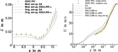
The modified set-up was designed such that the RANS models match the experimental values for ${\delta }^{\ast }$ at the two upstream reference positions. However, the RANS results for ${\delta }^{\ast }$ are not within the error bars of the experimental data in the region of non-equilibrium and strong APG. This deserves a few comments. The numerical uncertainty and the uncertainty of the computational set-up are not quantified. For example, the uncertainty of the input parameters (reference velocity, fluid viscosity and density) is not quantified. Another uncertainty stems from the 2D set-up, e.g. the displacement effect of the spanwise side wall boundary layers is not accounted for. Moreover, there is the delicate question about the small spanwise variation of δ due to inhomogeneities at the beginning of the test section (see [16]), which could contribute to the difference. Therefore, from Figure 5 (left) without such additional error bars, a lack of predictive accuracy of the RANS models cannot be rigorously concluded.

The impact of the computational set-up on the mean-velocity profile in the strong APG region at $x=9.944\mathrm{m}$ is shown in Figure 5 (right). The impact is of the same magnitude as the sensitivity with respect to the RANS model in the inner part of the boundary layer, i.e. by switching from SA to SA RC or from SSG/LRR-ω to SSG/LRR-ω-APG (being a modification for TBLs in APGs, see [37]). The misprediction in the outer part of the boundary layer is obvious for the original set-up, indicating an improper computational set-up.

Regarding implications for measurements, a single streamwise plane of inflow data was found to be not sufficient. Measurements for two or better multiple streamwise reference planes are strongly recommended. Additionally, at least one measurement plane just upstream of the region of interest (e.g. the beginning of the pressure gradient) is recommended.

3.3.2. 2D VT flow

The difficulty to account for the displacement effect of the side-walls on the flow in the centerplane for the 2D VT flow in a 2D computational set-up was studied by Fritsch et al. [11] and Eça et al. [34]. The parallel viscous top wall was replaced by an inviscid wall with a small inclination angle to account for the overall streamwise displacement effect. Additional simulations by Eça et al. [34] showed that the differences between the original set-up (parallel walls, viscous top wall) and the modified set-up were not significant for this flow. For comparison, note that for the DLR/UniBw flow, a small divergence angle between the top and bottom wall was used in the test section to account for the displacement effects of the side-wall boundary layers for the case of an empty test section.

Another issue is corner separation and the formation of horseshoe vortices at the junction of the test-model (NACA0012 airfoil) with the wind-tunnel spanwise side walls. A three-dimensional simulation of the full test-section including the viscous sidewalls is not necessarily a suitable way, due to the limitations of present RANS models to predict corner flow separation, thus introducing an additional model error. Preliminary simulations showed that, while linear eddy-viscosity models fail to capture the flow in corners and junctions, non-linear extensions like SA-QCR [10] gave qualitatively results closer to the measurements. It is worthwhile reporting that RANS simulations of the full 3D test section resolving the corner vortices for the experiment by Skare & Krogstad (see [48]) using differential Reynolds stress models are shown in [49]. Another subtle detail concerns the design of the corners of the wind tunnel. Note that secondary flow can be reduced if the corners are rounded. Concerning future experiments, in particular if a 2D separation is aimed at (see [16]), one could ask if junction flow separation should better be avoided or reduced in wind-tunnel experiments by using e.g. belly fairings used for commercial aircraft at the junction of wing and fuselage.

3.3.3. BeVERLI hill flow

For the BeVERLI Hill case, the question of symmetric versus asymmetric solutions of nominally symmetric flow arose, see [5]. At the higher hill-height-based Reynolds number ($R{e}_H=\mathrm{650,000}$) at a 45 degree orientation, the experiments showed a pronounced asymmetry in the separation region. At $R{e}_H=\mathrm{250,000}$, the flow exhibited a comparatively symmetric behavior during the experiment. For details see [5].

In regards to the CFD results, such asymmetry was found depending on grid refinement, turbulence model, and flow conditions. Under grid refinement a converged surface-flow topology was found, which was mainly determined by the RANS model. However, the behavior observed in the experiments could not be consistently replicated across all numerical setups. The results were contingent upon the numerical solver, CFD grid, and turbulence model employed. While experiments at 45 degree and $R{e}_H=\mathrm{250,000}$ showed a great level of symmetry, some simulations exhibited symmetry breaking. Similarly, at $R{e}_H=\mathrm{650,000}$, where experiments consistently displayed asymmetry, simulations produced a wide spectrum of results. This suggests that the flow asymmetry, inherent to the BeVERLI geometry, is influenced by both experimental boundary conditions and numerical factors. For further details, we refer to [13, 17] and to the companion paper [5] in this special issue.

Moreover, qualitative investigations into the stability of the asymmetric mode for the high-Re case were conducted, ruling out any bi-modal switching of the asymmetry. Additionally, it is noteworthy that at 0 degree orientation and $R{e}_H=\mathrm{650,000}$, both symmetry breaking and bi-modal switching were observed.

Some possible reasons for this need to be studied in future research. The asymmetry might be instigated by small asymmetries in the boundary conditions, including asymmetry in the oncoming flow. However, the triggering asymmetry could also be internally induced within the flow through a shear layer instability, akin to what is observed in the Ahmed body experiment. In the case of the BeVERLI Hill flow, it is plausible that the distinctively developing boundary layers around the flanks and over the top of the hill may be crossing and interacting on the leeward side of the hill, precipitating the instability and subsequently giving rise to the asymmetry.

3.3.4. Body-of-Revolution flow

Two main challenges were identified for predicting the flow around the BoR test case. The first one concerns the inlet condition. In the test section, the flow is fully developed and all RANS turbulence models are designed to predict a law-of-the-wall velocity profile in a fully developed pipe flow. However, both the experimental data and the DNS simulation results revealed the existence of a marked wake profile near the center of the pipe similar to what can be observed in a developing flow over a flat plate, possibly due to the existence of persisting anisotropic coherent turbulent structures in this region. To obtain the inlet profiles for the numerical RANS simulation, it was found necessary to use an ad-hoc blending approach to combine the inner RANS solution of a fully developed pipe flow with the DNS results in the outer region. Moreover, even with such an inlet condition, it was found that the eddy-viscosity turbulence models fail to maintain the inlet profile over a long enough distance before reaching the body. An ad-hoc forcing term needs therefore to be added in the momentum equations in the region between the inlet and the body to take artificially into account the existence of this wake region and to reduce the error due to the inlet condition. It is worthwhile to notice that such a forcing term is not needed when the Reynolds-Stress Transport model SSG-LRR is used.

The second challenge is the modelling of the highly accelerated flow around the curved leading edge resulting from a very strong favorable pressure gradient. Any eddy-viscosity model fails to predict correctly the flow in this region. With a very poor prediction in the fore-body region, the assessment of eddy-viscosity based turbulence model in the region further downstream becomes difficult. The SSG-LRR model can provide a significantly better prediction in the strongly accelerated region around the leading edge. Unfortunately, further downstream, it performs similarly to the linear eddy-viscosity models. For the BoR test case, the turbulence modelling error is so high that the effect of grid resolution is of secondary influence. The corresponding results for the longitudinal mean velocity profile and the turbulent Reynolds shear stress in two different regions (fore-body and mid-body) are described and discussed in the companion paper on the three-dimensional test cases [5].

3.4. Quantitative tools for assessment of errors and uncertainties

Two exemplary studies using quantitative tools for the assessment of errors and uncertainties are described. In Section 3.4.1, the work by Oberkampf and Smith [23] was followed in a detailed investigation of the BeVERLI Hill flow by Gargiulo et al. [13]. For this purpose, the grid dependence of the simulations was further analysed to assess the numerical uncertainty caused by the discretisation error, as described below. In Section 3.4.2, the work by V&V-20-Committee [33] and Eça et al. [1] was pursued for the 2D VT flow by application of the quantitative method of the Standard for Verification and Validation in CFD (V&V 20).

3.4.1. Quantitative study of the uncertainty due to discretisation error

For the BeVERLI Hill flow, the grid dependence of a solution was utilised to estimate the discretisation error (DE). Such was elaborated in [13], wherein principles drawn from Roache [21], grounded in Richardson extrapolation, are applied.

The method is tailored for implementation on a set of at least three systematically refined grids, each with a refinement factor denoted by r. In this framework, the assumption is made that other sources of error, such as iterative and round-off errors, are negligible compared to DE. Note that, if iterative errors cannot be reduced to negligible levels, it is useless to perform grid refinement, since iterative errors can mask grid effects. Additionally, it is assumed that DE approaches zero asymptotically with increasing grid refinement. Under these conditions, the discretisation error, ${\overline{\epsilon }}_h$, can be estimated by employing Richardson extrapolation for a given solution, u, computed on a grid with a spacing of h: (6) ${\overline{\epsilon }}_h=\frac{u_{\mathrm{rh}}-u_h}{r^{p_f}-1}.$(6) Here, $p_f$ is the formal order of accuracy associated with the discretisation scheme.

If the aforementioned framework assumptions are not met, the solution can exhibit a different observed order of accuracy (OOA), $\hat{p}$, that deviates from the formal order $p_f$. If the solutions are asymptotic, however, $\hat{p}\approx p_f$. The OOA can be estimated as (7) $\hat{p}=\frac{\ln \left(\frac{u_{r^{2}h}-u_{\mathrm{rh}}}{u_{\mathrm{rh}}-u_h}\right)}{\ln \left(r\right)}.$(7) It should be mentioned that this equation assumes that the refinement ratio between medium and coarsest grid is exactly equal to the refinement ratio between finest and medium. Because the OOA often deviates from $p_f$ in practice, $\hat{p}$ is used instead in Equation (6(6) ${\overline{\epsilon }}_h=\frac{u_{\mathrm{rh}}-u_h}{r^{p_f}-1}.$(6) ).

Note that if the solutions fail to converge monotonically towards the asymptotic value, e.g. as observed in the oscillating converging solutions from the VT RANS simulations of the BeVERLI Hill case, the OOA becomes undefined, necessitating the implementation of additional precautions. To estimate the DE in such scenarios, a methodology akin to the one proposed by Phillips and Roy [50] can be applied. Their method advocates for averaging the locally computed OOA at designated Richardson nodes, representing grid points where the OOA is well-defined, to obtain a global OOA. The global OOA is then used to calculate the DE as outlined in Equation (6(6) ${\overline{\epsilon }}_h=\frac{u_{\mathrm{rh}}-u_h}{r^{p_f}-1}.$(6) ).

Once computed, the DE error can be used again using Richardson extrapolation to provide an uncertainty to the solution. The uncertainty due to DE (denoted by $U_{\mathrm{DE}}^{f_i}$) for a flow quantity f obtained on grid level i (denoted by $f_i$) is then estimated as (8) $U_{\mathrm{DE}}^{f_i}=F_s\cdot |f_i-f_{\mathrm{Richardson}}|$(8) where $F_s$ is a factor of safety accounting for the fact that the underlying assumptions for the estimation of DE are not perfectly met and the Richardson extrapolated solution, $f_{\mathrm{Richardson}}=f_1+(f_1-f_2)/(r^{p_{\mathrm{glb}}}-1)$ (with $p_{\mathrm{glb}}$ being the global OOA), which uses the solution on the finest available level $f_1$ on GL1 and $f_2$ on GL2.

Alternatively, Roache suggests a grid convergence index GCI to provide an error band on the grid convergence of the solution. (9) $U_{\mathrm{DE}}^{f_i}=\frac{F_s}{r^{p_{\mathrm{glb}}}-1}\cdot |f_i-f_{i+1}|$(9) Similarly, the uncertainty due to the DE can be obtained for the $C_p$ and $C_f$ distributions. For details see [13]. For illustration, Figure 6 shows $C_p$ and $C_f$ on all grid levels GL1 to GL4 for the ${45}^{\circ }$ yaw case BeVERLI Hill at $R{e}_H\approx 650,000$.

Figure 6. $C_p$ and $C_f$ along the centerline in the streamwise $x_1$-direction (left) and the centerspan in the spanwise $x_3$-direction (right) from the ${45}^{\circ }$ yaw case BeVERLI Hill at $R{e}_H\approx \mathrm{650,000}$ on grid levels GL1 to GL4 (from [13]; reprinted by permission of the American Society of Mechanical Engineers ASME). Note that $x_1\equiv x$ and $x_3\equiv z$ in Figure 2 (left). The dotted line shows the hill geometry.

The uncertainty due to DE is illustrated in Figure 7.

3.4.2. Application of the V&V 20 standard for verification and validation

The ASME V&V 20 standard was applied in [34] to the 2D VT flow. The estimation of the model error using Equation (1(1) $E-U_{\mathrm{val}}\le {\delta }_{\mathrm{model}}\le E+U_{\mathrm{val}}$(1) ) demands estimates of the discretisation error $U_{\mathrm{DE}}$ (being $U_{\mathrm{num}}$ in Section 2.5), the experimental error $U_{\mathrm{D}}$, and the input error $U_{\mathrm{inp}}$. Note that, as a 2D simulation of the VT flow is considered, the modeling error ${\delta }_{\mathrm{model}}$ includes a contribution of the domain geometry even if complete inlet boundary conditions were available from the experiments (if the ‘strong-model’ option is applied, see Subsection 2.5). For the input uncertainty, the following contributions were considered: the location of the inlet boundary, the tilting angle of the top wall, and the airfoil angle of attack (if the exact value is not known, or is likely to be altered due to the 3D flow conditions in the test section). The input uncertainty $U_{\mathrm{inp}}$ was estimated based on numerical tests. For example, the contribution of the uncertainty due to the design of the top wall in the computational set-up was estimated by comparing the simulation results for the set-up with an inviscid top wall with a tilting angle and a viscous parallel top wall.

Figure 7. Uncertainty due to the discretisation error (DE) in $C_f$ along the centerline in $x_1$-direction (top) and the centerspan in $x_3$-direction (bottom) of the ${45}^{\circ }$ yaw case BeVERLI Hill at $R{e}_H\approx \mathrm{650,000}$ for SA-model (left) and SST-model (right) (from [13]; reprinted by permission of the American Society of Mechanical Engineers ASME). Note that $x_1\equiv x$ and $x_3\equiv z$ in Figure 2 (left). The dotted line shows the hill geometry.

For the evaluation of the uncertainty due to the discretisation error, the baseline meshes by VT and the airfoil-refined meshes were assessed. The aim was to study the effects of the flow around the airfoil on the flat plate. It was found that too coarse meshes in the vicinity of the airfoil may lead to apparently small uncertainties [36] that significantly underpredict the real uncertainty as suggested by the results obtained with the airfoil-refined grid set by MARIN/IST [34, 36]. This indicates a possible danger for the estimation of the numerical uncertainty. The numerical solution can show a weak dependence on the refinement level, if the mesh in a critical flow region (here: near the airfoil), which is of large importance for the overall flow field, is so coarse, that the grid dependence is weak. Hence the baseline mesh used for a global refinement study needs to be sufficiently fine in all relevant flow regions.

For illustration, Figure 8 (left) shows the uncertainty bars of the discretisation error $U_{\mathrm{num}}$ for $C_{\mathrm{f}}$ for the SST model for two different families of meshes (baseline meshes by VT and meshes with refinement around the airfoil by MARIN/IST (MI)). Then Equation (1(1) $E-U_{\mathrm{val}}\le {\delta }_{\mathrm{model}}\le E+U_{\mathrm{val}}$(1) ) is used to estimate the differences between the $C_f$ distributions obtained with six turbulence models ${\delta }_{\mathrm{TM}}$ using the SST 2003 (see [51]) solution as the reference data (D) and taking into account the numerical uncertainties. The non-overlapping error bars in the non-equilibrium region for the model-scale Re indicate that the differences due to the RANS model are significant compared to the other uncertainties. Moreover, the results for the full-scale Re are included. For the high Re, the role of the RANS model becomes smaller. This will be discussed in more detail in the next subsection.

Figure 8. Left: Uncertainty bars of the discretisation error for $C_f$ for the SST model for two different families of meshes (baseline meshes by VT and meshes with refinement around the airfoil by MARIN/IST (MI)). Right: Estimate of the error of the turbulence model ${\delta }_{\mathrm{tm}}$ for $C_f$ with reference model SST 2003 for model-scale $\mathrm{Re}=2\times {10}^6$ and for full-scale $\mathrm{Re}={10}^9$(Figures reprinted from [34]).

3.5. Extrapolation from model-scale to full-scale Re

There is an additional validation problem due to the lack of experimental data at full scale. To study this, a purely numerical investigation was performed for the 2D VT flow by comparing the results for $R{e}_c=2\times {10}^6$ and $R{e}_c={10}^9$, despite the absence of wind-tunnel data (see [34]). (It is worthwhile to recall that $R{e}_x$ based on the development length x of the boundary layer on the wind-tunnel wall is much larger).

At full scale Re, a much clearer separation between the inner layer and the outer layer is reached. The extent of the log-law region is ${10}^2<y^{+}<5\times {10}^5$ compared to ${10}^2<y^{+}<{10}^3$ for $R{e}_c=2\times {10}^6$, and the RANS models SA, SST and SSG/LRR-ω almost perfectly collapse in the log-law region. For the high Re, the history effects and the effect of the RANS model are seen only in the law-of-the-wake region. The mean velocity in the log-law region remains unaltered due to the streamwise pressure gradient, and so do the turbulence quantities. On the other hand, for $R{e}_c=2\times {10}^6$ (despite the large value of $R{e}_x$), the log-law region is still relatively thin, and changes in the law-of-the-wake region due to the streamwise pressure gradient are also leading to changes in the outer part of the log-law region (see Figure 9 and [34]). However, this finding might not extend to cases with turbulent flow separation. The main finding is that differences between different RANS models become smaller in the limit of very high Reynolds number. This leads to the conjecture that the role of the RANS model becomes smaller for full scale simulations, at least as far as the contribution of non-equilibrium TBLs and mild pressure gradients are concerned.

Figure 9. Mean velocity profiles in viscous units for the 2D VT flow at model-scale $\mathrm{Re}=2\times {10}^6$ and at full scale $\mathrm{Re}={10}^9$ at $x=3.5\mathrm{m}$ for the airfoil incidence angles $\alpha =-{10}^{\circ }$ (left), $\alpha =0^{\circ }$ (middle), and $\alpha ={12}^{\circ }$ (right)(Figures reprinted from [34]).

3.6. Interim assessment of the role of the RANS turbulence model

The above subsections attempted to illustrate the different sources of uncertainties and their relative contribution to the deviation between the numerical solution of RANS models and the experimental data for different CFD-validation experiments. The variability due to the RANS turbulence model was found to be much larger than the influence of the CFD grid, provided that the CFD grid ensures an acceptable level of numerical uncertainty. On the other hand, the uncertainty due to the computational set-up, in particular for a nominally 2D flow, can be of the order of the model error of the turbulence model. The uncertainty due to the measurement technique (and possibly the post-processing to infer QoIs) can also be significant. The findings of this summary are discussed in more detail in the following subsection.

3.7. Discussion

The uncertainties can be categorised into three levels. The uncertainty level UL1 is proposed to describe uncertainties, which are quantifiable and controllable in magnitude, and which can be made sufficiently small or even negligible (compared to the other uncertainties). An uncertainty can be called quantifiable, if reliable bounds for the uncertainty can be given. An uncertainty is (loosely speaking) called controllable, if expertise in measurement technique and/or CFD can control its magnitude and keep it below a given (reasonable) bound. The uncertainty due to the mesh is of level UL1, given sufficient expertise in mesh generation and computing resources. For 2D simulations, a global hierarchical mesh refinement can be used. For most 3D simulations, at least a suitable local mesh refinement is possible. (However, in such cases, it becomes more difficult to quantify the numerical uncertainty.) Similarly, the measurement uncertainty and the uncertainty in the method to determine QoIs using post-processing are (in principle) of level UL1. For example, the measurement resolution can be chosen to accurately resolve the most sensitive quantities, e.g. the Reynolds stresses. Sometimes, a more sophisticated and elaborate method could be needed (i.e. OFI for $C_f$ instead of a Clauser chart method). In reality, restrictions in time, budget and/or measurement equipment often prevent one from reaching the desired accuracy. At any rate, the uncertainties of level UL1 should be made as small as possible compared to the other uncertainties. The required efforts, diligence and time are a highly effective investment at only moderate extra costs (in particular compared to the efforts of a reliable improvement of RANS models [37]).

The other extreme is level UL3, being associated with the model error of the RANS model, for which exact error bounds cannot be given at the present state. First rough estimates for the bounds might be possible using e.g. a Monte-Carlo type approach from a sensitivity analysis of different terms of the model equations. In such an analysis, the inherent relations among the different coefficients within a RANS turbulence model due to the calibration for decaying isotropic turbulence, free shear flows and the log law at zero pressure gradient need to be accounted for (see [52, 53]). This topic is beyond the scope of the present work.

An uncertainty level UL2 in between could be assigned to the uncertainty due to the flow conditions in the computational set-up compared to the test section of the wind tunnel. This uncertainty is in part due to a lack of knowledge of the boundary conditions in the wind tunnel (completeness and exactness of the data) imposed in a 3D computational set-up (however, it interferes with the model error, as described below). Therefore, the flow conditions in the inlet and exit plane of the test section need to be known exactly. Uncertainties arise due to a deviation between nominal and actual free-stream conditions, a non-zero boundary-layer thickness at the inlet, and flow inhomogeneities across the inlet plane. Such inhomogeneities are often caused upstream of the test-section inlet and can be due to flow separation in the region of the turning vanes or details of the flow behaviour in the region of the screens.

An additional uncertainty arises, if the effect of the boundary conditions on the flow in the region of interest cannot be exactly reproduced by the computational set up in combination with the model error due to the RANS model. An example for this is the overprediction of corner flow separation by a linear eddy-viscosity model for a 3D set-up of the 2D VT flow and the effect on the flow in the centerplane of the test section. Therefore, even for a full 3D set-up, an indirect input error due to the RANS model arises.

Another issue arises due to an inhomogeneity of the flow at the entrance into the test section. Then the boundary layers on the wind-tunnel walls can be differently influenced by such inhomogeneities. Such non-homogeneities can persist far downstream in the wind tunnel (see [54]) and can lead to spanwise asymmetric corner-flow/junction-flow separation. Moreover, such non-homogeneities and their streamwise evolution can often depend on the free-stream velocity. For first results for the DLR/UniBw flow, see [16]. In RANS simulations, however, such inhomogeneities are likely to be damped too rapidly in the streamwise direction.

A 2D computational set-up of a 3D validation experiment introduces additional uncertainties, which are very difficult to quantify. One aspect is the difficulty to describe the displacement effects of the spanwise wind-tunnel wall boundary layers, in particular, if the flow at the spanwise walls is not attached and corner flow separation and vortical flow occurs.

The first main conclusion is to make all possible efforts to keep the uncertainties due to the CFD grids and the measurement technique as small as possible. Some ideas how this could be achieved are described in Section 4.2.

The second major conclusion is that the largest uncertainty apart from the RANS model error stems from uncertainties due to the computational set-up. However, there are different sources of uncertainties involved. Some uncertainties can be significantly reduced by careful measurements and by a CFD-friendly design of the wind-tunnel experiment, as described in Section 4.2.

4. Possible paths for future research

This section attempts to describe two possible paths to tackle the challenges and open questions. Future needs for CFD-mesh generation and refinement are proposed in 4.1. Ideas for future experiments for CFD validation at high Re are discussed in 4.2.

4.1. Future needs for CFD-mesh generation and refinement

The uncertainty associated with the CFD mesh is the one for which the largest progress at relatively low effort can be achieved, given the large increase in available computing resources. A viable way would be a combination of best-practice guidelines for grid design and convergence studies together with some new features provided by mesh-generation tools. A useful feature would be the automatic generation of mesh families satisfying some refinement metrics (as described in Section 3.1). Moreover, automatic methods to check the accuracy of the geometry model (as-built versus the as-designed) could be provided at reasonable efforts.

For 3D complex flows, families of globally refined meshes may become too large. Local mesh refinement in critical flow regions is a viable route. For mesh adaptation, robust and reliable refinement metrics are needed, and optimal methods for refining the mesh such as node movement and cell sub-division are still not available. The adaptive use of higher-order methods is also a potential avenue for solution adaptation.

For complex 3D flows, hybrid meshes using hexahedral elements in boundary layers and prismatic and tetrahedral elements elsewhere can be used. Metrics to assess the mesh quality compared to pure hexahedral meshes are needed. There is a special importance of mesh refinement studies for 3D flows with smooth body separation.

Best-practice guidelines for the required mesh spacing in streamwise, wall-normal, and spanwise directions seem to be extremely dependent on what is happening in the specified flow of interest, and one could be skeptical about a general implementation using geometrical information alone inside the mesh-generation tool. From characteristic parameters (Reynolds number, length of viscous-wall boundaries), information about the design of the boundary-layer mesh (boundary-layer thickness, viscous scaling for $y^{+}(1)$) could be inferred. From the geometry information together with a RANS solution, estimates about the streamwise/lateral variation of the pressure gradient and curvature could be made, yielding information on the streamwise/lateral spacing. Such would require the possibility to use and analyse CFD solutions inside the mesh generator.

From the view point of a design engineer, a high level of automation of the mesh-generation process, without (significant) need for user intervention and manual work, is desirable, in particular if CFD is used as part of a design optimisation framework.

4.2. Future experiments for CFD validation at high Reynolds numbers

The uncertainties of the computational versus the experimental set-up and of the measurement data are seen to have the largest potential for reaching a new level of reliable experiments for the validation and improvement of turbulence models, not only for RANS models, but also for wall-modelled LES methods.

Future needs regarding the wind-tunnel facility and the measurement technique are summarised in [23], proposing a detailed list of assessment criteria for CFD model validation experiments. The systematic fulfillment of their highest quality level 3 would lead to a drastical improvement in validation experiments. The findings by the AVT-349 regarding the requirements for the inflow and outflow conditions confirm the proposal by Oberkampf and Smith [23]. Although such painstaking work might not seem to be of the highest interest for researchers interested in improving measurement technology or discovering new flow physics models, it is of the highest relevance for a reliable validation experiment.

The need for detailed information of the boundary conditions became obvious during the course of AVT-349. Some aspects could be studied within the time-frame and the scope of this project, but larger future activities and collaborations are needed. Large-scale measurements, if possible, over the full cross section of the test section are an elaborate task. Such task was performed in part for the DLR/UniBw experiment [16] and is in progress at a higher detail level for the VT wind-tunnel (AVT-387). The quantification of the flow in the empty test-section (flow homogeneity, turbulence level), also near the side walls and in the corners, is important. Such measurements also need to be performed with mounted test-models, as pressure gradients can change (amplify) non-homogeneities of the flow, and at the different conditions during the wind-tunnel measurements (e.g. at different values for the free-stream velocity). Large-scale measurements could also help elucidating the flow in the junction of wind-tunnel wall and test model to get information on the size of corner vortices.

Regarding the measurement technique, the level-3 requirement by Oberkampf and Smith [23] suggests the use of different high-quality techniques to measure the same quantity, and to use different set-ups and calibrations. This implies the recommendation to complement PIV with LDV or hotwire, and to compare different PIV set-ups, e.g. two-component measurements in a plane (2D2C), stereo PIV (2D3C), and possibly the use of Lagrangian particle tracking (LPT). Moreover, a systematic resolution study (e.g. by a reduction of the field of view of PIV) could be used in a way similar to a grid convergence study for CFD. The analysis of the PIV data within AVT-349 confirmed that there is still a strong need in future research on measurement techniques for high-Re turbulent-boundary-layer flows with their large spatial dynamic range from the smallest viscous length scale to the largest scale (the boundary-layer thickness). LPT demonstrated to be a promising candidate (see [12] for the DLR/UniBw flow). Measurements of the mean velocity in the viscous sublayer for a direct determination of the wall shear stress would be helpful, but there are many technical difficulties (wall reflections, uncertainty of the wall distance, roughness due to seeding particle size). Oil-film interferometry is a useful alternative (although some technical issues arise for low local velocities, e.g. near separation). Again, a complementary use of two techniques is expected to lead to the highest overall accuracy and reliability (see [23]).

Validation experiments (in particular for 2D flows) should make best use of the wind-tunnel. A large spanwise extent of the test section compared to the boundary-layer thickness (not much smaller than around 9:1) could reduce the displacement effect of the side walls significantly. Flow separation in regions other than the regions of interest should be avoided. For example, junction flow separation could be avoided using belly fairings used for commercial aircrafts in the junction of wing and fuselage.

For the reduction of the experimental uncertainties, RANS-based CFD could be a valuable partner. New wind-tunnel campaigns should be joint activities between experts for wind-tunnels, measurement techniques, turbulence and its modelling, and CFD, in close cooperation during all stages from the planning phase until the final evaluation of the measurement results. For the design of the experiment, characteristic flow parameters in the test-section and in the regions of interest as Re, boundary-layer thickness, strength of the pressure gradient, and the tendency for flow separation can be estimated. Moreover, the experimental resolution requirements (for the mean velocity and Reynolds stresses in the inner part of the BL and for $C_f$) can be estimated. Third, RANS can be used to define regions of interest for detailed measurements and identify the need for special local modifications of the wind-tunnel or the test model, e.g. the position of a glass insert for optical access for PIV. Finally, RANS is a helpful reference during the evaluation of the measurement data. For all these aspects, RANS-based CFD was used to assist the DLR/UniBw experiment (see [12, 16]).

Information about 3D-flow effects in the test section (junction flows, corner separation, generation of vortices, transport of inflow inhomogeneities) could be obtained complementary from turbulence-resolving numerical simulations like hybrid RANS/LES or (embedded) wall-modelled LES. Hybrid RANS/LES methods are amenable for high-Re flows (in particular for flows at incompressible conditions) and could be complemented by RANS simulations using second-moment closure models or a non-linear constitutive relation, e.g. SA with QCR-extension [10]. Quantitative information about the 3D flow in the test section could be used to define a simplified computational 2D set-up for the flow in the centerplane.

Finally, as a short-term strategy, the dependence of the results on specifics of a certain wind-tunnel can be checked by testing the same geometry model in different wind-tunnels (at the same flow conditions, if possible). In the present initiative, the BeVERLI Hill flow was studied in different wind-tunnels at Virginia Tech and SINTEF Ocean/UTIAS. This was found to be very valuable to confirm critical observations of the flow field such as asymmetry.

Best-practice recommendations and a check-list of how to reach a good computational set-up of quasi 2D wind-tunnel experiments are needed. Best-practice guidelines should include the findings of AVT-349, i.e. measurement of inflow data at several streamwise positions, using a large spanwise extent of the test section compared to the boundary-layer thickness (with a ratio of at least 9:1), and ensuring near-equilibrium flow approaching the exit of the test section.

To summarize, future experiments for CFD validation could be significantly improved by a rigorous application of the guidelines for the experimental facility and the measurement technique in [23]. A detailed quantification of the facility (as pursued within AVT-387) is recommended. The use of RANS simulations can help to design the wind-tunnel experiment and to select the measurement technique. Finally, special guidelines to reduce the uncertainties in the wind tunnel (as sufficient spanwise aspect ratio for nominal 2D flows, measures to avoid unnecessary flow separation), and the complementary use of hybrid RANS/LES and/or (embedded) wall-modelled LES to shed light on the flow conditions in critical parts of the test-section are suggested.

5. Summary and conclusions

For the conclusions, first a summary is given on what was learned from the work within AVT-349, what can be confirmed from the present stage of knowledge, and what can/should already be accounted for in CFD studies. Then the issues that are not fully clear yet and need future research are described. Finally, paths for future work and expectations along with major needs for future research activities and efforts are summarised.

Regarding the uncertainty due to the CFD grid, strategies for a systematic mesh-refinement study (e.g. a family of 5, or even better 7 to 9 meshes, using a refinement ratio of $2^{1/2}$ for 2D flows, which might be weakened to $2^{1/3}$ for 3D flows) and mesh refinement metrics are available and should become part of the CFD culture. The meshes need to be fine enough to capture all features of the flow. For locally too coarse meshes, there is a danger that the solution does not capture all details. This can be inferred from being too far from the asymptotic range for grid convergence, i.e. the observed order of accuracy is not near the formal order. Put in other words, one is too far from monotonic convergence to enable a reliable estimate of the exact solution with an acceptable observed order of accuracy. Moreover, the observed order of accuracy needs to be studied for each boundary part individually (e.g. $C_p$ for the airfoil in the 2D Virginia Tech experiment needs to be studied separately from $C_p$ at the bottom wind-tunnel wall). Besides that, it is important to check that the solution does not exhibit local oscillations, as this could also cause problems for the estimation of the discretisation error.

The automatic generation of families of systematically refined meshes satisfying such metrics would be a worthwhile feature to be provided by software tools for mesh generation. Estimation of the uncertainty bars for the discretisation error (e.g. by using a Richardson extrapolation) is useful. For non-equilibrium flows, the mesh resolution requirements were observed to be increased compared to equilibrium flows at the same Re.

In addition to the spatial discretisation error which was the focus of this article (as all test cases yielded a steady-state solution), time-dependent flow problems introduce a temporal discretisation error. Moreover, a statistical convergence uncertainty is introduced, if flow statistics are computed.

The uncertainty due to the CFD grid for the simulation of wind-tunnel experiments of non-equilibrium turbulent-boundary layers was assessed by reference to the other uncertainties. The uncertainty due to the measurements and the post-processing for the quantities of interest was found to be increased in non-equilibrium flow regions and at high Re compared to flows near equilibrium at moderate Re. It was confirmed that a sufficient number of streamwise measurement stations for mean velocity and Reynolds stresses in the non-equilibrium regions is needed to track the streamwise changes. For high-Re flows, the spatial resolution requirements for the Reynolds stresses in the inner part of the boundary layer become demanding, and can be estimated from RANS results before the measurement campaign. Keeping these uncertainties as small as possible was found mandatory before assessing the uncertainties due to the computational set-up and the RANS model.

The two major sources of uncertainties were found to be the RANS turbulence model and the flow conditions in the test section for the numerical/computational set-up compared to the wind-tunnel. The latter are due to uncertainties and differences in the boundary conditions (CFD versus wind-tunnel). For nominally 2D flows, the uncertainty of the computational set-up was found to be larger than for 3D flows. Adjustments of the computational 2D set-up were found to be needed, but require special care and expert knowledge, and best-practice guidelines are strongly needed.

Quantitative tools (V&V 20) could help the assessment of errors and uncertainties. The detailed list of assessment criteria for CFD model validation experiments by Oberkampf and Smith [23] and the exemplary studies for the BeVERLI Hill flow in [13] and for the NASA juncture flow experiment [24] as well as a rigorous uncertainty quantification, exemplified e.g. in [46], should become part of the culture for joint experimental-computational work, as well as the lessons learned for cooperation and communication of the different disciplines involved (experimentalists, computors and other, as described in [24]). However, a simplified systematic approach for a CFD engineer seems to be needed, along with a check-list of best-practice guidelines. Moreover, such knowledge and check-list needs to be transferred to the community of CFD engineers at industry and research establishments. Workshops and courses as well as invited talks at conferences could foster such transfer. Moreover, a central database to provide useful information could be helpful. A new section for the category of CFD model validation experiments proposed by Oberkampf and Smith [23] might become part of an international webpage, e.g. the turbulence modeling resource webpage² by NASA, listing good examples of validation cases satisfying the criteria by Oberkampf and Smith [23] as well as other useful documents for verification and validation. This webpage could provide at least a bibliography of such cases and perhaps more data, if they can be made publicly available for the CFD community.

Without an uncertainty analysis, there is a danger of a too optimistic assessment of a RANS model (due to cancellation of errors) as well as being too pessimistic (if the uncertainties due to the measurement accuracy and due to the computational set-up are not distinguished from and hence attributed to the model form error of the RANS turbulence model).

Regarding the ultimate aim to quantify the error of a given RANS turbulence model, the work of AVT-349 confirmed that reliable error bars for all sources of uncertainties (other than the RANS model error) are required. Then a reliable quantification of empirical error bars of different RANS models can be given. However, empirical error bars of RANS models are very likely to be test-case specific.

This leads to possible paths for future research. Concerning the CFD mesh, relatively large improvements could be achieved by enabling mesh-generation tools for suitable families of systematically refined meshes fulfilling grid metrics. Adaptive local mesh refinement strategies exploiting information from a given RANS solution have a large potential for 3D complex configurations, as shown in e.g. AVT-301 [55].

The greatest potential for the reduction of the uncertainties of CFD-validation experiments was found for the computational versus the experimental set-up. Detailed and complete measurement data in the entire inlet and outlet plane of the wind-tunnel test section were found of utmost importance. The computors need to prioritize the need for boundary condition data to be measured by the experimentalists, and to describe what is most important to know for a specific experiment to characterise the boundary layer. Inflow data at several streamwise positions (ranging from near the beginning of the test section to a little upstream of the non-equilibrium region of interest) to track the streamwise evolution of the flow were found to be important. For this purpose, it was found that data for the mean velocity profile from the logarithmic layer up to the boundary-layer edge at several streamwise positions was more useful than highly resolved data down to the wall at a single position. Internal flows require special care regarding the information needed about the mean velocity and the Reynolds stresses. This topic shows the high relevance of the initiative on ‘Common Research Wind Tunnels for CFD Verification and Validation’ of AVT-387. High-quality hybrid RANS/LES and/or wall-modelled LES of the 3D flow in the entire wind-tunnel (or in crucial flow regions, e.g. corner flow separation) could be used to complement such experimental data and to estimate sensitivities of the system response coefficients. Such an estimation of uncertainties of system response quantities in the wind-tunnel centerplane by numerical simulation (e.g. due to corner flow and its prediction by different RANS models like SA, SA-RC-QCR and RSM versus turbulence resolving methods) might also be a useful future task.

Validation experiments should be made CFD-friendly. Validation experiments for 2D flow are still attractive for RANS model calibration and application of machine-learning methods. Flow separation should be avoided, unless it is the target flow phenomenon, as an asymmetric 3D flow can arise in the test-section. Unwanted or complicated separation could be avoided or reduced by a 3D CFD design, e.g. fairings to avoid corner flow separation. A large aspect ratio of wind-tunnel span to boundary-layer thickness can help keep the effect of the spanwise side walls small (in case that a 2D set-up is aimed at).

Another important aspect deserving efforts in future research is the role of Reynolds number effects, as the RANS models are mainly validated for test cases at model-scale Re (e.g. ${10}^6$, see [34]), but need to be applied for designs operating at Reynolds numbers of several orders of magnitude higher (e.g. ${10}^9$).

It is worthwhile to point out that the comments made about the experimental setup are directed towards wind-tunnel tests and applications. Therefore, they may be less interesting for the maritime community where towing tanks are commonly used. Some of the wind-tunnel challenges do not appear in towing tanks. E.g. when testing a submarine in a wind tunnel, there are issues with the inflow definition, boundary layer build up and pressure gradient along the flow axis, while during towing a submarine in a towing tank, the flow is stationary, no boundary layer builds up on the tank walls and there is a constant ambient pressure. On the other hand, there are other issues (such as a free surface) when using a towing tank. Put in other words, it may be worth saying that wind-tunnel testing is not the only way to obtain validation data.

Finally, it is worthwhile outlining the impact of the above findings for the use of CFD for the design of complex civil and military air and sea vehicles. Flow separation on a submarine hull and on an aircraft wing is often largely influenced by the upstream non-equilibrium turbulent-boundary layer. Beyond adverse/favourable pressure gradients and curvature, the flow around a transport aircraft or a fully appended submarine encounters also junction flows, corner separations, tip vortices, etc. The needs to capture the non-equilibrium boundary-layer flows and the onset of flow separation using a well-designed CFD grid and a carefully chosen RANS model remain a crucial part of CFD simulations, near the design point and for off-design flow conditions. The remaining (and still not quantifiable) error of the RANS model underlines the need for future research activities on the physics and modelling of non-equilibrium turbulent-boundary-layer flows (as pursued in the AVT-ET-234/AVT-RTG-413 ‘Physics and Modelling of Separated Flows Around Smoothly-Curved Bodies’).

Acknowledgments

The very valuable discussions within the AVT-349 are gratefully acknowledged. Special thanks are to W. Devenport and H. Babinsky for leading this initiative.

Disclosure statement

No potential conflict of interest was reported by the author(s).

Additional information

Funding

T. Knopp gratefully acknowledges funding by the DLR internal aeronautical program within the project ADaMant. The DLR/UniBw experiment was funded by Deutsche Forschungsgemeinschaft (DFG) (Grant KA 1808/14-1 & SCHR 1165/3-1), by the DLR Institute of Aerodynamics and Flow Technology, and by the DLR program directory board within the DLR internal projects VicToria. The authors from Virginia Tech would like to thank Dr. Peter Chang and Dr. Julie Young of the Office of Naval Research for their support under grant numbers N00014-18-1-2455,N00014-19-1-2109, and N00014-20-2821. We would also like to thank the U.S. Department of Defense High Performance Computing Modernisation Program (HPCMP) for computational resources. The research by MARIN is partly funded by the Dutch Ministry of Economic Affairs.

Notes

1 https://turbmodels.larc.nasa.gov/

2 https://turbmodels.larc.nasa.gov

References

- Eça L, Dowding K, Roache PJ. On the interpretation and scope of the V&V 20 standard for verification and validation in computational fluid dynamics and heat transfer. J Verif Valid Uncertain Quantif. 2022;7:021005.
- Oberkampf WL, Roy CJ. Verification and validation in scientific computing. Cambrigde: Cambridge University Press; 2010.
- García-Mayoral R, Chung D, Durbin P, et al. Challenges and perspective on the modelling of high-Re, incompressible, non-equilibrium, rough-wall boundary layer. J Turbul. 2024.
- Klewicki J, Sandberg R, Knopp T, et al. On the physical structure, modeling and computation-based prediction of two-dimensional, smooth-wall turbulent boundary layers subjected to streamwise pressure gradients. J Turbul. 2024.
- Lowe KT, Smits A, Visonneau M, et al. Effects of streamline curvature and three dimensionality). J Turbul. 2024.
- Spalart PR, Allmaras SR. A one-equation turbulence model for aerodynamics flows. In: AIAA Paper 1992-0439, Reno, NV; 1992.
- Menter FR. Two-equation eddy-viscosity turbulence models for engineering applications. AIAA J. 1994;32:1598–1605. doi: 10.2514/3.12149
- Eisfeld B, Rumsey C, Togiti V. Verification and validation of a second-moment-closure model. AIAA J. 2016;54:1524–1541. doi: 10.2514/1.J054718
- Shur ML, Strelets MK, Travin AK. Turbulence modeling in rotating and curved channels: assessing the Spalart-Shur correction. AIAA J. 2000;38:784–792. doi: 10.2514/2.1058
- Spalart PR. Strategies for turbulence modelling and simulation. Int J Heat Fluid Flow. 2000;21:252–263. doi: 10.1016/S0142-727X(00)00007-2
- Fritsch D, Vishwanathan V, Roy CJ, et al. Experimental and computational study of 2D smooth wall turbulent boundary layers in pressure gradient. In: AIAA Paper 2022-0696, San Diego (CA); 2022.
- Knopp T, Reuther N, Novara M, et al. Experimental analysis of the log law at adverse pressure gradient. J Fluid Mech. 2021;918:A17 24A17–1–A17 –32. doi: 10.1017/jfm.2021.331
- Gargiulo A, Duetsch-Patel JE, Borgoltz A, et al. Strategies for computational fluid dynamics validation experiments. J Verif Valid Uncertain Quantif. 2023;8(3):Paper no. VVUQ 24Paper no. VVUQ–23–1011, 1–25 .
- Ding L, Saxton-Fox T, Hultmark M, et al. Effect of pressure gradient and streamline curvature on the statistics of a turbulent pipe flow. In: Eleventh International Symposium on Turbulence and Shear Flow Phenomena (TSFP11); Southampton (UK): University of Southampton; 2019. p. 353–358.
- Visonneau M, Deng G, Guilmineau E, et al. Bodies-of-revolution in turbulent flow: comparing computation with experiment. In: AIAA Paper 2022-0694, San Diego (CA); 2022.
- Knopp T, Schanz D, Novara M, et al. Experimental and numerical investigation of turbulent boundary layers with strong pressure gradients. In: AIAA Paper 2022-1035, San Diego (CA); 2022.
- Gargiulo A, Ozoroski TA, Hallock T, et al. Computations of the BeVERLI Hill three-dimensional separating flow model validation cases. In: AIAA Paper 2022-1034, San Diego (CA); 2022.
- Oberkampf WL, Trucano TG. Verification and validation in computational fluid dynamics. Albuquerque and Livermore: Sandia National Laboratories; 2002. (Technical report).
- Roache PJ. Quantification of uncertainty in computational fluid dynamics. Annu Rev Fluid Mech. 1997;29:123–160. doi: 10.1146/fluid.1997.29.issue-1
- Roache PJ. Error bars for CFD. In: AIAA Paper 2003-408, Reno, NV; 2003.
- Roache PJ. Fundamentals of verification and validation. Socorro, New Mexico: Hermosa Publishers; 2009.
- Roy CL. Errors and uncertainties: their sources and treatment. In: Beisbart C, Saam NJ, editors. Computer Simulation Validation: Fundamental Concepts, Methodological Frameworks, and Philosophical Perspectives; Cham: Springer; 2019. p. 119–141.
- Oberkampf WL, Smith BL. Assessment criteria for computational fluid dynamics model validation experiments. J Verif Valid Uncertain Quantif. 2017;2:031002. doi: 10.1115/1.4037887
- Rumsey CL. Insights and lessons learned from the NASA juncture flow experiment. J Aircr. 2022;59(6):1493–1499. doi: 10.2514/1.C036838
- NATO AVT-246 Task Group. Progress and challenges in validation testing for computational fluid dynamics. 2016 Sep. (NATO MP-AVT-246 Report).
- Patel VC. Calibration of the Preston tube and limitations on its use in pressure gradients. J Fluid Mech. 1965;23:185–208. doi: 10.1017/S0022112065001301
- Heyse JF, Mishra AA, Iaccarino G. Estimating RANS model uncertainty using machine learning. J Glob Power Propuls Soc. 2021;1–14. doi: 10.33737/jgpps/134643
- Oliver TA, Moser RD. Bayesian uncertainty quantification applied to RANS turbulence model. J Phys Conf Ser. 2011;318:042032. doi: 10.1088/1742-6596/318/4/042032
- Wang Q, Dow EA. Quantification of structural uncertainties in the k-ω turbulence model. Phys Fluids. 2010;14:2043–2051. doi: 10.1063/1.1476668
- Xiao H, Cinnella P. Quantification of model uncertainty in RANS simulations: A review. Prog Aerosp Sci. 2019;108:1–31. doi: 10.1016/j.paerosci.2018.10.001
- Volino R, Fritsch D, Devenport W, et al. Effects of roughness on non-equilibrium turbulent boundary layers. J Turbul. 2024.
- Nikuradse J. Strömungsgesetze in rauhen Rohren. Berlin: 1933. (Technical report, VDI-Forschungsheft 361).
- V&V-20-Committee. Standard for verification and validation in computational fluid dynamics and heat transfer. American Society of Mechanical Engineers; 2009. (Technical report).
- Eça L, Kerkvliet M, Toxopeus SL. Comparison of RANS turbulence models for the simulation of smooth wall boundary-layers in pressure gradient at moderate and high Reynolds numbers. In: Garcia-Espinosa J, Gonzalez L, Gutierrez JE, Servan-Camas B, editors. 10th International Conference on Computational Methods in Marine Engineering (MARINE 2023); Madrid, Spain; 2023.
- Eça L, Hoekstra M, Windt J. Practical grid generation tools with applications to ship hydrodynamics. In: 8th International Conference on Numerical Grid Generation in Computational Field Simulations; Honolulu, Hawaii, USA; 2002.
- Eça L, Kerkvliet M, Toxopeus SL. Turbulent boundary layers with variable pressure gradient using RANS. IST, Lisboa, Portugal: Universidad de Lisboa; 2022. (Technical report, Tech. Rep. M-10).
- Knopp T, Reuther N, Novara M, et al. Modification of the SSG/LRR-omega model for adverse pressure gradients. Flow Turbul Combust. 2023;111:409–438. doi: 10.1007/s10494-023-00457-8
- Bailey SCC, Hultmark M, Monty JP, et al. Obtaining accurate mean velocity measurements in high Reynolds number turbulent boundary layers using pitot tubes. J Fluid Mech. 2013;715:642–670. doi: 10.1017/jfm.2012.538
- Atkinson C, Buchmann NA, Amili O, et al. On the appropriate filtering of PIV measurements of turbulent shear flows. Exp Fluids. 2014;55:1654. doi: 10.1007/s00348-013-1654-8
- Kähler CJ, Scharnowski S, Cierpka C. On the resolution limit of digital particle image velocimetry. Exp Fluids. 2012;52:1629–1639. doi: 10.1007/s00348-012-1280-x
- Kähler CJ, Scharnowski S, Cierpka C. On the uncertainty of digital PIV and PTV near walls. Exp Fluids. 2012;52:1641–1656. doi: 10.1007/s00348-012-1307-3
- Herpin S, Wong CY, Stanislas M, et al. Stereoscopic PIV measurements of a turbulent boundary layer with a large spatial dynamic range. Exp Fluids. 2008;45:745–763. doi: 10.1007/s00348-008-0533-1
- Vishwanathan V, Fritsch DJ, Devenport WJ, et al. Spatial resolution limitations of particle image velocimetry in high Reynolds number turbulent boundary layers. Preprint Version 1. Research Square, 2022. doi: 10.21203/rs.3.rs-2384035/v1.
- de Silva CM, Gnanamanickam EG, Atkinson C, et al. High spatial range velocity measurements in a high Reynolds number turbulent boundary layer. Phys Fluids. 2014;26:025117. doi: 10.1063/1.4866458
- Novara M, Schanz D, Reuther N, et al. Lagrangian 3D particle tracking in high-speed flows: shake-the-box for multi-pulse systems. Exp Fluids. 2016;57:Article ID 128, 1 24Article ID 128, 1–20 . doi: 10.1007/s00348-016-2216-7
- Bailey SCC, Vallikivi M, Hultmark M, et al. Estimating the value of von Kármán's constant in turbulent pipe flow. J Fluid Mech. 2014;749:79–98. doi: 10.1017/jfm.2014.208
- Thibault R, Poitras GJ. Uncertainty evaluation of friction velocity measurements by oil-film interferometry. J Fluids Eng. 2017;139:051401. doi: 10.1115/1.4035461
- Skare PE, Krogstad PA. A turbulent equilibrium boundary layer near separation. J Fluid Mech. 1994;272:319–348. doi: 10.1017/S0022112094004489
- Sporschill G. Improved Reynolds-stress modeling for adverse-pressure-gradient turbulent boundary layers in industrial aeronautical flow [PhD thesis]. Universite de Pau et des Pays de l'Adour; 2021.
- Phillips TS, Roy CJ. Richardson extrapolation-based discretization uncertainty estimation for computational fluid dynamics. J Fluids Eng. 2014;136(12):121401. doi: 10.1115/1.4027353
- Menter FR, Kuntz M, Langtry R. Ten years of industrial experience with the SST turbulence model. In: Turbulence, Heat and Mass Transfer 4; West Redding: Begell House; 2003. p. 625–632.
- Durbin PA, Petterson Reif BA. Statistical theory and modelling for turbulent flows. Chichester: John Wiley & Sons; 2001.
- Menter FR, Matyushenko A, Lechner R. Development of a generalized k-ω two-equation turbulence model. In: Dillmann A, Heller G, Krämer E, Wagner C, Tropea C, Jakirlic S, editors. New Results in Numerical and Experimental Fluid Mechanics. Contributions to the 21st STAB/DGLR Symposium Darmstadt, Germany 2018; Vol. 142; Cham: Springer; 2018. p. 101–109.
- Marusic I, Chauhan KA, Kulandaivelu V, et al. Evolution of zero-pressure-gradient boundary layers from different tripping conditions. J Fluid Mech. 2015;783:379–411. doi: 10.1017/jfm.2015.556
- NATO AVT-301 Task Group.Flowfield prediction for manoeuvring underwater vehicles. 2022 Jun. (NATO TR-AVT-301 Report).