Macroeconomic assessment of India’s development and mitigation pathways

ABSTRACT

Although a rapidly growing economy, India faces many challenges, including in meeting the Sustainable Development Goals of the United Nations. Moreover, post-2020 climate actions outlined in India’s Nationally Determined Contribution (NDC) under the Paris Agreement envision development along low-carbon emission pathways. With coal providing almost three-quarters of Indian electricity, achieving such targets will have wide-ranging implications for economic activity. Assessing such implications is the focus of our research. To do so, we use a hybrid modelling architecture that combines the strengths of the AIM/Enduse bottom-up model of energy systems and the IMACLIM top-down economy-wide model. This hybrid architecture rests upon an original dataset that brings together national accounting, energy balance and energy price data. We analyse four scenarios ranging to mid-century: business-as-usual (BAU), 2°C, sustainable 2°C and 1.5°C. Our 2°C pathway proves compatible with economic growth close to the 6% yearly rate of BAU from 2012 to 2050, at the cost of reduced household consumption but with significant positive impact on foreign debt accumulation. The latter impact stems from improvement of the trade balance, whose current large deficit is the primary cause of high fossil fuel imports. Further mitigation effort backing our 1.5°C scenario shows slightly higher annual GDP growth, thereby revealing potential synergies between deep environmental performance and economic growth. Structural change assumptions common to our scenarios significantly transform the activity shares of sectors. The envisioned transition will require appropriate policies, notably to manage the conflicting interests of entrenched players in traditional sectors like coal and oil, and the emerging players of the low-carbon economy.

Key policy insights

• Low carbon pathways are compatible with Indian growth despite their high investment costs

• Moving away from fossil fuel-based energy systems would result in foreign exchange savings to the tune of $1 trillion from 2012 to 2050 for oil imports.

• Achieving deep decarbonization in India requires higher mobilized capital in renewables and energy efficiency enhancements.

• Phasing out fossil fuels would, however, require careful balancing of interests between conventional and emerging sector players through just transitions.

KEYWORDS:

• India
• energy-economy model
• sustainable development
• 2°C
• 1.5°C
• climate policy

Introduction

Since economic liberalization in 1991, India’s GDP has been growing at an annual rate of 7% to 8%. Part of this growth stems from structural change, which saw the Indian economy turn from agriculture in the 1970s, to services and industry, which contributed 53% and 31% of GDP respectively in 2017 (Economic Survey, 2018). This drive is expected to continue, with governmental policies like Make in India, Smart Cities Mission and Housing for All providing impetus to the manufacturing sector and infrastructure development. Services should also benefit from public programmes like Digital India and Start-up India.

Despite this robust growth trend, India faces many socio-economic challenges resonating with the Sustainable Development Goals (SDGs) of the United Nations. Nearly 300 million people are still living in poverty (MoSPI, 2018) and without access to electricity (NEP, 2017). About 50% of rural households lack basic socio-economic services (SECC, 2015). Per capita energy consumption is only one third of the global average (IEA, 2015), which betrays low levels of energy services. The SDGs must, however, be balanced with national targets for greenhouse-gas emissions abatement. In its nationally determined contribution (NDC) submitted under the Paris Agreement, India has committed to reducing the emission intensity of its GDP 33% to 35% below its 2005 level by 2030, and to scaling up its non-fossil share of power capacity to 40% (MoEFCC, 2015). This commitment should be seen in the context of coal currently contributing to nearly three quarters of power generation, and fossil fuels more generally meeting three quarters of total energy demand. Moreover, Indian energy demand is expected to grow exponentially following rapid urbanization, industrialization and the rising purchasing power of the population. By mid-century, India is projected to be among the world’s largest national energy consumers (IEA, 2018). Decarbonizing energy supply will require substantial investment costs, whereas it should improve the trade balance, in a context where oil imports amount to 80% of the current trade deficit (ETEnergyWorld, 2018). Our research aims to analyse the balance of such losses and gains, that is, the ultimate macroeconomic impacts of low-carbon development pathways for India.

Numerous studies have investigated the implications of decarbonization strategies on the energy system and economic development of India (Dubash, Khosla, Rao, & Sharma, 2015; Parikh & Parikh, 2011; Shukla, Dhar, & Mahapatra, 2008; Shukla & Chaturvedi, 2012; van Ruijven et al., 2012). Gambhir, Napp, Emmott, and Anandarajah (2014) investigate the financial and other potential benefits of decarbonization using the TIMES bottom-up model of energy systems. They compare Indian mitigation costs with global average costs to determine potential revenues from the sale of international carbon credits. Byravan et al. (2017) also implement the TIMES model to compare the GHG emissions, primary energy demand, investment costs and energy imports requirement of a business-as-usual (BAU) versus a sustainable development scenario. Multiregional studies like Fragkos and Kouvaritakis (2018), Van Soest et al. (2017) and Vandyck, Keramidas, Saveyn, Kitous, and Vrontisi (2016) underline the large emission gap between the NDC and 2°C pathways for India using a global energy system model. Vishwanathan, Garg, and Tiwari (2018; Vishwanathan, Garg, Tiwari, & Shukla, 2018) apply the AIM/Enduse bottom-up model to determine the challenges and opportunities involved in limiting global warming to 2°C and below. Chaturvedi, Koti, and Chordia (2018) implement the GCAM integrated assessment model to analyse 216 scenarios combining key technical uncertainties characterizing mitigation strategies. However, all these technology-rich studies lack economy-wide coverage, that is, they overlook feedbacks of energy constraints on economic activity and hence energy demand.

Top-down approaches provide such coverage. Van Soest et al. (2016) and Saveyn, Paroussos, and Ciscar (2012) use the multiregional Computable General Equilibrium (CGE) model GEM-E3 to discuss the economic implications of energy efficiency measures and the penetration of carbon-free technologies in a 2°C scenario. Another recent study by Mittal, Liu, Fujimori, and Shukla (2018) assesses the mitigation costs of achieving global temperature stabilization well below 2°C and 1.5°C, using the AIM CGE model. However, both models are global and represent India as one region among many, in a standard CGE framework of perfect markets ill-suited to the country’s specificities. They also lack the technology-rich information of bottom-up approaches to frame their outlooks on India’s energy futures.

This underlines the need for hybrid models that combine the strengths of top-down (TD) and bottom-up (BU) approaches (Hourcade, Jaccard, Bataille, & Ghersi, 2006). Pradhan and Ghosh (2012) make some attempt in this direction by building an original social accounting matrix and combining a CGE model with a global climate model to analyse the impact of carbon taxes and emissions trading on GDP growth. However, they fail to take account of energy flow statistics at any stage of their modelling endeavour. Shukla et al. (2008), Fragkos et al. (2018) or Vishwanathan, Fragkos, Fragkiadakis, Paroussos, and Garg (2019) deploy soft-coupling strategies between BU models and TD models, but limit them to the one-way feeding of BU information into their TD models and do not consider feedbacks.

Our research attempts at further bridging the gap between BU and TD assessments of Indian development pathways. We develop a hybrid architecture that couples the AIM/End-use model of Indian energy systems and the IMACLIM model of the Indian economy and considers the feedback loops between the two tools. Additionally, IMACLIM-IND calibrates upon an original dataset reconciling national accounting, energy flow and energy price data. We apply the AIM/Enduse and IMACLIM architecture to the exploration of four scenarios: BAU, 2°C, sustainable 2°C, 1.5°C, to determine the implications of mitigation strategies on the energy systems and the economy of India. The second section of our paper outlines the methodology and data backing our analysis. The third section describes the architecture of our scenarios. The fourth section presents and discusses scenario results while the fifth section concludes.

Methodology

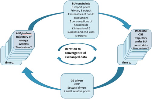
The conventional bottom-up and top-down approaches have been opposed since the 1990s (Grubb, Edmonds, ten Brink, & Morrison, 1993). While standard top-down models are incapable of incorporating technical information on energy systems, bottom-up models do not account for the macroeconomic costs, description of investment markets and feedbacks between macroeconomic aspects and the transition of energy systems. To generate a consistent picture of the Indian energy-economy system, we resort to model coupling through the iterative exchange of outputs and inputs up to numerical convergence, as discussed in Ghersi (2015). This convergence method has been used in the past, for example in the Swedish (Krook-Riekkola, Berg, Ahlgren, & Söderholm, 2017) and Portuguese (Fortes, Simões, Seixas, Van Regemorter, & Ferreira, 2013) contexts. With this method, we couple the bottom-up AIM/Enduse model with the top-down IMACLIM-IND model of the Indian economy (Figure 1). The coupling process starts with IMACLIM-IND running under constraint of AIM/Enduse assumptions and results on energy import prices, fossil energy output, the capital intensities of energy transformation sectors and energy intensive non-energy sectors, the energy intensities of activity sectors, the energy consumption of households, energy exports and capital intensities of various sectors. IMACLIM-IND computes various economic indicators like sectoral outputs, household income or aggregate GDP, which it then feeds back to AIM/Enduse to update energy demand trends. The process is repeated 2–3 times until the exchanged data converges. Appendix C reports on how convergence affects both model outputs and demonstrates the advantage of iterating to convergence over one-way linking.

Figure 1. Iteration process.

A precondition to the relevance of such coupling was the construction of an original dataset hybridizing extensive energy/economy data from various sources (see Appendix A). The resulting dataset (Gupta, Ghersi, & Garg, 2018a) has the advantage of acknowledging the heterogeneity of energy prices faced by different economic agents, as recorded by energy statistics. IMACLIM reflects this heterogeneity by considering agent-specific sales margins (Gupta, Ghersi, & Garg, 2018b). Both data hybridization and the heterogeneity of energy prices have non-marginal impacts on policy evaluation (Combet, Ghersi, Lefèvre, & Le Treut, 2014; Le Treut, 2017).

The dataset (and consecutively IMACLIM-IND) discriminates 8 energy sectors and 14 non-energy sectors (Table 1) based on their energy intensities and policy relevance. The iron & steel, cement, chemical & petrochemical, textile and aluminium sectors are targets of energy efficiency initiatives by the Government of India.

Table 1. IMACLIM-IND sectors.

Energy Sectors (8)	Model nomenclature	Non- energy sectors (14)	Model nomenclature
Coal	COAL	Iron & Steel	IRONSTEEL
Coke	COKE	Chemical & petrochemical	CHEMPETROCHEM
Crude oil and non-transport fuels	OILNTFUEL	Aluminium	ALUMINIUM
Transport fuels	TRANSPFUEL	Cement	CEMENT
Biomass	BIOMASS	Construction	CONSTRUCTION
Natural gas	NATURALGAS	Textile	TEXTILE
Electricity	ELECTRICITY	Residual industries	RESIDINDUSTRIES
Renewable Energy^a	RENEWABLE	Agriculture	AGRICULTURE
		Air transport	AIRTRANSP
		Water transport	WATERTRANSP
		Road transport	ROADTRANSP
		Rail transport	RAILTRANSP
		Housing	HOUSING
		Other services	OTHERSERVICES

^aThe Renewable Energy sector groups solar, wind, nuclear and hydrogen power-generation options. Its only use is as Electricity sector input.

The AIM/Enduse BU model provides a techno-economic perspective at the national level along with sectoral granularity. It is a linear cost-optimization model based on technology selection. The total cost of the Indian energy system is minimized under constraints of service demand, energy resource availability and material and other system constraints (Kainuma, Matsuoka, & Morita, 2011). AIM/Enduse outputs cover energy demands, energy efficiency, capital intensity and technology substitution across sectors. Vishwanathan, Garg, Tiwari et al. (2018) and Vishwanathan et al. (2017) provide a detailed description of the assumptions and parameters backing the Indian AIM/Enduse model. The model has been calibrated to energy-economy data up to 2015 and runs in annual time steps to 2050. It is updated with new technologies including smart grids, electric vehicles, Carbon Capture, Utilization and Storage (CCUS), battery storage, improved coal technologies like Integrated Gasification Combined Cycle (IGCC), Pulverized Coal (PC) or Ultra Super Critical Coal (USCC) and advanced renewable technologies like solar with storage.

The IMACLIM model is a multi-sectoral dynamic recursive model¹ that pictures economic growth as proceeding from exogenous increases of labour supply and labour productivity. It is specifically designed to accommodate exogenous BU information on energy supply, demand and trade (Ghersi, 2015), thereby renouncing micro-foundation of the producers’ and consumer’s energy supply and consumption behaviours in favour of forced technical coefficients. IMACLIM-IND extends the process to the capital intensity of important non-energy sectors, building on the annualized investment costs per unit output reported by AIM/Enduse for the iron & steel, cement, chemical & petrochemical, textile and aluminium sectors. Considering our implementation in single time steps from 2012 to 2030 and 2050, IMACLIM-IND renounces the ad hoc calibration of the standard accumulation rule and simplifies capital accumulation by assuming that the capital stock grows proportionally to investment flows, which are an exogenous share of GDP.² The consequence is that capital stock grows broadly in pace with efficient labour endowment (the dominant GDP driver). The rental price of capital adjusts to clear capital markets, considering substitution possibilities with labour in those sectors not informed by AIM/Enduse for their capital intensities.

IMACLIM-IND has two other specific features with important bearing on its results and their interpretation. The first is a flexible trade balance, to allow assessment of the impact of low-carbon pathways on trade, considering the weight of energy imports at the 2012 base year (10.0% of GDP). The standard model of a fixed (balanced) trade via flexible terms-of-trade effectively translates trade variations into general activity. We rather strive to estimate how our scenarios affect the current large trade deficit without forcing any exogenous trade balance outcome. Trade flexibility requires some assumption regarding the terms-of-trade. IMACLIM-IND adjusts them to force the purchasing power of the average wage to increase at the same pace as labour productivity. This is the condition for a stable unemployment rate (at its 2012 level) following a ‘wage curve’ specification acknowledging the observed correlation between the unemployment rate and the real average wage (Blanchflower & Oswald, 2005). The policy interpretation of this specification is that of the Government of India taking measures to control the Indian exchange rate with a view to stabilize unemployment.

A second specific feature of IMACLIM-IND is its choice of macroeconomic closure. Rather than considering some exogenous savings rate and closing on investment (neoclassical closure of the standard CGE model), IMACLIM-IND considers a fixed investment effort (‘Johansen closure’ following Sen, 1963) and closes on the households’ saving rate – taking account of the foreign saving capacity induced by the flexible trade balance. This specification means to reflect the significant level of intervention of the government of India in economic affairs: the government controls the country’s investment trajectory by adjusting its net transfers to households, either in the form of fiscal (public income) or social (public expenditure) reforms.

The consequence of both features is that the interpretation of IMACLIM-IND results differs from that of standard models. Notwithstanding the absence of a welfare index (which flows from the forcing of BU-sourced energy consumptions), the fixed investment trajectory induces stability of GDP via stability of capital accumulation across mitigation scenarios. Household consumption adjustments, which in effect finance this stability of GDP, are more relevant indicators of economic performance. However, the flexible trade balance also matters as it implies differentiated accumulation of foreign debt across scenarios. Consequently, we systematically report these two indicators when commenting upon our scenario results (see Section 4). Gupta et al. (2018b) provide a complete online description of the model.

Scenario description

We apply the modelling architecture of Section 2 to explore four scenarios corresponding to increasing energy-system constraints. Our business-as-usual (BAU) scenario builds on the prolongation of current trends and provides the benchmark of our analyses. Our 2 degree (2DEG) scenario and its 2 degree Sustainable (2DSUS) variant consider Indian mitigation action compatible with a global temperature increase at 2°C above pre-industrial levels. Our 1.5DEG scenario considers Indian action compatible with the stricter global cap of a 1.5°C increase of the global average temperature. All scenarios build on Indian labour force projections of the United Nations Population Division, which increase the total labour force from 512 million workers in 2015 to 744 million in 2050 (Table 2). They also share assumptions on labour productivity gains that stem from the governmental Economic Survey 2017–18, as well as international energy price assumptions from the New Policy Scenario of the 2015 World Energy Outlook (IEA, 2015).³ The following subsections comment upon the mitigation measures and behavioural assumptions backing each scenario.

Table 2. Scenario assumptions.

	BAU	2DEG	2DSUS	1.5DEG
Labour endowment	+1.57% per year from 2013 to 2030 then +0.72% per year from 2030 to 2050
Labour productivity	+4.9% per year from 2013 to 2030 then +4.8% per year from 2030 to 2050
Policy measures	NDC targets, advanced renewables and energy efficiency targets, NAPCC, cut in subsidies in fossil fuels, ethanol blending; Housing for all; Power for all; Smart Grid Mission	Advanced NDC; CCS in power sector and industries; Early retirement of inefficient coal plants; Clean coal technologies; Aggressive PAT targets; Smart Cities Mission; AMRUT; Smart metres; EVs	Coal power phase-out by 2050; CCS only in industry sector; Aggressive PAT targets; Smart Cities Mission; AMRUT; Smart metres; EVs	More renewables; More CCS, BECCS, clean coal technologies, more aggressive PAT targets; Aggressive PAT targets; Near zero EE building; Smart Cities Mission; AMRUT; Smart metres; EVs
Behavioural changes	Switch to efficient lighting, cooling, vehicles.	Public transport, dematerialization, waste recycling, work from home.	More public transport, dematerialization, waste recycling, work from home.	More public and shared transport, dematerialization, waste recycling, work from home.

AMRUT: Atal Mission for Rejuvenation and Urban Transformation.

Business as usual (BAU) scenario

Our BAU scenario reflects current energy-economy system dynamics under constraint of the public policies of the National Action Plan on Climate Change (NAPCC) (PMCoCC, 2008), the draft National Electricity Plan (NEP) (2017), the Indian NDC (MoEFCC, 2015) and the Perform Achieve Trade (PAT) scheme – a market-based mechanism for energy intensive industries to trade energy-saving certificates. NAPCC includes eight national missions led by various ministries in the areas of Solar Energy, Sustainable Habitat, Sustainable Agriculture, Enhanced Energy Efficiency, Water, Green India, Sustaining the Himalayan Ecosystem and Strategic Knowledge for Climate Change. These national plans set the broad objectives for all 32 States/Union Territories of India to prepare their respective State Action Plans on Climate Change (SAPCC).

Under its NDC, India has committed to two major quantitative objectives, namely, reducing national emission intensity to 33–35% below its 2005 level in 2030, and raising the contribution of non-fossil fuels to 40% of total power capacity by 2030 (MoEFCC, 2015). Under the NAPCC, the Government of India (GoI) sets additional goals that include creating smart grids, improving the power system, building sustainable infrastructure and buildings, and generating on-grid and off-grid renewable power from sources like solar, wind, small hydro and bioenergy. All these goals are met endogenously in AIM/Enduse by way of capacity and technology-share constraints. These include increasing the modal share of railways and metros, the building of dedicated freight corridors and the penetration of electric vehicles (EVs). Households turn to energy-efficient technologies like solar cooking stoves. For details on implementation of policies sector by sector see Appendix B.

Low-carbon scenarios

The design of the 2DEG and 2DSUS scenarios builds on policies that allow containing Indian CO₂ emissions within a 115–147 billion tons (Bt) CO₂ budget between 2011 and 2050 (CD-Links, 2019; Tavoni et al., 2014), while in the BAU scenario it goes up to 165 Bt CO₂. This is line with global models (van den Berg et al., 2019), which set a range of 90–125 Gt-CO₂. Though our analysis is limited to CO₂ emissions outside those from afforestation, reforestation and land-use change, other emissions are important for India, particularly CH₄ emissions from agriculture and livestock, which employ the majority of the Indian population. India also aims to increase its carbon sinks through afforestation. In fact, the Indian forested area has increased over recent years due to the national policies of sustainable forest management and afforestation. The 2DEG scenario does not put any constraint on coal use, which leads to coal remaining the mainstay of the Indian energy system. The 2DSUS scenario on the other hand assumes complete phase-out of coal in power generation by 2050.

The 1.5DEG scenario envisions further measures still, which cap the 2011–2050 carbon budget below the 115 Bt CO₂ estimated as India’s share of a global 1.5°C-compatible budget (CD-Links, 2019; van den Berg et al., 2019). Using the carbon constraint option in AIM/Enduse model, the model endogenously picks up more efficient coal and gas technologies, renewables and micro-grids based on cost optimization and technology availability. Energy intensive sectors like aluminium, steel or cement see their activities reduce thanks to developments in material sciences that could change the profile of end-use materials as we know them today. They pick up transformative technologies like switching to pulverized coal injection and top recovery turbine in the iron & steel sector. This implies increased capital intensities, which AIM duly reports and which we use to shape the capital intensity trajectories of some non-energy sectors in IMACLIM. The 1.5DEG scenario is based on the premise that technology and behavioural lock-ins are avoided and that carbon-saving technical change happens from the very beginning of our time horizon.

Scenario results

Converging AIM/Enduse and IMACLIM-IND without any assumption on market instruments inducing the modelled transformations amounts to considering a command-and-control implementation of scenario constraints. The optimization framework of AIM additionally implies that the policy maker has perfect information regarding the merit order of energy supply and end-use technologies.

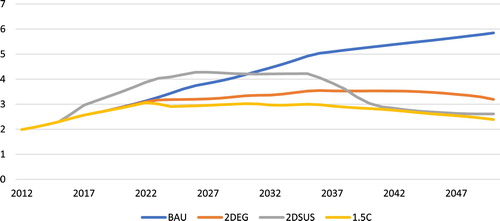
Under such conditions, the four scenarios generate contrasting CO₂ emission profiles (Figure 2). Under BAU, unconstrained CO₂ emissions increase throughout the modelled horizon to reach 6 Bt in 2050. In the 2DEG scenario, emissions slow down their increase after 2020 and start declining after 2035, although at a slow pace. In the 2DSUS scenario, the ban of CCS in the power sector and the prospect of coal power phase-out by 2050 induce a surge of emissions in early years, indeed above BAU levels. This surge is caused by power generation turning to coal options in the early years, to avoid stranding coal-mining assets. Emissions then plateau after 2025 and decline sharply after 2035, to converge with the 1.5DEG emission trajectory around 2040. The latter trajectory is unsurprisingly the lowest one, with emissions plateauing as early as 2022 and further declining after 2035 with cumulative CO₂ emissions from 2012 to 2050 being 105 BtCO₂ in this scenario. Those of the 2DEG and 2DSUS scenarios are similar at slightly higher levels, 123 and 131 BtCO₂ respectively. Our results for CO₂ emissions fall well within the ranges obtained from the effort-sharing approaches of van den Berg et al. (2019). They are also in line with Indian emissions in the CD-Links (2019) scenario database for both our horizon years, although at the higher end of the range outlined by the database. For a ‘high probability’ of staying below 2°C warming, CD-Links places 2050 Indian emissions between 1.1 and 3.5 BtCO₂. At the same 2050 horizon, the range decreases to between 0.35 and 2.5 Bt CO₂ for a 1.5°C scenario.

Figure 2. Indian CO₂ emissions, GtCO₂.

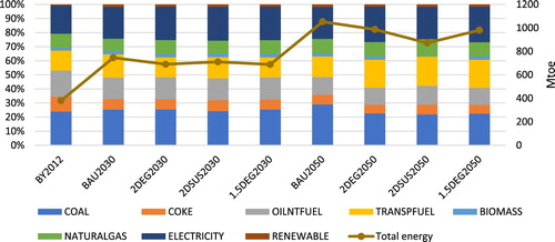
Coal sees its share increase in the final energy consumption of non-energy sector firms up to 2050 in BAU, while it eventually decreases in all low-carbon scenarios, although remaining above 20% (Figure 3). At the end horizon, all energy vectors similarly contribute to the decrease of total firm consumption, with the marked exception of transportation fuels, which therefore see their share increase. Biomass consumption develops in the 2DEG and 1.5DEG scenarios when backed by CCS, but disappears in the 2DSUS scenario with the CCS ban. The CD-Links database suggests that the non-fossil fuel share in total energy use increases significantly to reach nearly 90% in 2050 for both the 2°C and 1.5°C objectives. Our numbers rather suggest that fossil fuels will continue to play a bigger role, even though less significant than at the base year, in the 2050 Indian economy.

Figure 3. Final energy consumption of productive sectors.

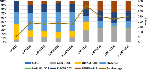
The energy mix of household consumptions evolves towards less biomass and more renewables in BAU (Figure 4). This reflects the AIM/Enduse assumption that households who currently depend on inefficient fuelwood as the main source of energy for cooking gradually switch to LPG and electricity. Our analysis includes CO₂ emissions related to unsustainable fuelwood use. It is particularly important for India (see appendix A) where the majority of rural households uses biomass as a cooking fuel. Unsustainable biomass uses like heating and cooking cause air pollution and high black carbon leading to negative health consequences for women and children in particular. In all three low-carbon scenarios, transportation fuels see their share decline dramatically, reflecting the forced development of public transport. This is supported by Dhar, Pathak, and Shukla (2018) emphasizing the role of clean fuels, technology innovations and changes in end-use demand in the transport sector for a 1.5°C pathway.

Figure 4. Final energy consumption of households.

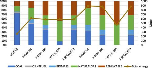
In the power generation mix, the contributions of natural gas, renewables and biomass increase while that of coal declines in the BAU scenario (Figure 5). In low-carbon scenarios, the share of renewables ends up exceeding 30%, and even 50% in the 2DSUS scenario, to compensate for the coal-power phase-out. Generation from coal reaches its peak value much earlier in 2DSUS compared to 2DEG due to that constraint. Power generation then switches to gas and renewables (including nuclear) in shares reflecting the compared costs and capacity constraints of each technology. In all low-carbon scenarios but particularly in the 2DSUS scenario, autonomous energy efficiency improvements translating the penetration of storage technologies, net metering, smart grids and micro grids and demand-side management decrease power generation requirements. A study by Van Soest et al. (2017) also shows the share of low-carbon energy sources in total energy supply increasing up to 32% in 2030 for a cost-optimal 2°C scenario.

Figure 5. Energy inputs into power generation.

Although inducing contrasting energy systems, the four scenarios show minor GDP variations, within 0.7% in 2050 and barely noticeable if expressed as variations of the average annual growth rate (Table 3 and 4). However small, the GDP differences are systematically in favour of the low-carbon scenarios compared to BAU. The major cause for this result – beside the balance of energy-efficiency improvements and their capital costs – is the stability of the investment effort measured in GDP points across scenarios (Johansen closure, see Section 2). The carbon intensity of GDP consecutively drops, from 0.4 in BAU to 0.16 in 1.5DEG, measured in tons of CO₂-equivalent (tCO₂) per thousand 2010 USD. Our number for carbon intensity for 2DEG2030 is on the lower end of the range of 0.69–0.79 tCO₂ per thousand USD of the CD-Links database while for 2DEG2050 the results are aligned.

Table 3. Macroeconomic results of four scenarios, 2030.

	BY2012	BAU 2030	2DEG 2030	2DSUS 2030	1.5D 2030
Real GDP (Trillion 2012 USD)	1.740	5.188	5.510	5.525	5.510
Average annual growth rate (2013 onwards)		6.26%	6.61%	6.63%	6.61%
Annual CO2 emissions (Bt CO2)	1.99	4.18	3.34	4.21	3.02
CO2 intensity of GDP (tCO2/10^3 USD)	1.14	0.81	0.61	0.76	0.55
Hholds’ consumption (GDP share)	59.6%	70.6%	65.6%	66.2%	65.6%
Foreign debt (GDP share)	128.0%	197.0%	101.7%	115.7%	101.7%
Trade balance (GDP share)	−7.42%	−12.14%	−7.12%	−7.78%	−7.11%
E imports (GDP share)	−10.0%	−11.7%	−6.8%	−7.6%	−6.8%
E exports (GDP share)	3.6%	1.7%	1.7%	1.7%	1.7%

Table 4. Macroeconomic results of four scenarios, 2050.

	BY2012	BAU 2050	2DEG 2050	2DSUS 2050	1.5D 2050
Real GDP (Trillion 2012 USD)	1.740	14.707	14.992	15.064	15.006
Average annual growth rate (2013 onwards)		5.78%	5.83%	5.84%	5.83%
Annual CO2 emissions (Bt CO2)	1.99	5.85	3.19	2.61	2.39
CO2 intensity of GDP(tCO2/10^3 USD)	1.14	0.40	0.21	0.17	0.16
Hholds’ consumption (GDP share)	59.6%	66.4%	64.8%	64.5%	64.6%
Foreign debt (ratio to GDP)	128.0%	204.9%	133.0%	118.1%	121.8%
Trade balance (GDP share)	−7.42%	−7.99%	−6.39%	−6.07%	−6.14%
E imports (GDP share)	−10.0%	−7.3%	−5.4%	−4.7%	−5.0%
E exports (GDP share)	3.6%	2.3%	2.3%	2.1%	2.2%

The scenarios affect the share of household consumption in GDP in ways that nuance these GDP results. They decrease this share by 4.4–5.0 percentage points in 2030 and by 1.6–1.9 percentage points in 2050.⁴ This is the direct consequence of the increased trade balance i.e. decreased foreign savings under the assumption of Johansen closure on consumption (see Section 2). Indeed, mitigation has a strong impact on the trade balance, whose deficit recedes by up to 5 percentage points in 2030 and 1.8 percentage points in 2050, compared to BAU. In 2050, the weight of energy imports shifts from 7.3% of GDP, to 5.4% in the 2DEG scenario, 5% in the 1.5DEG and 4.7% in the 2DSUS scenario. This is an obvious consequence of the decline of fossil fuel energy uses like that of oil fuels in the transport sector, of natural gas in industry and of high-grade coal in steel production. Crude oil and other refined fuel imports decline from a 26% share of total imports in the base year to a 15% share in 1.5DEG in 2050. This amounts to foreign exchange savings of 620 billion USD over 2012–2030 from a reduction in just oil imports in the 2DEG scenario compared to BAU, and savings close to 1 trillion USD from 2012 to 2050. Through this impact on energy trade, mitigation positively affects the foreign debt of India by constraining it below or only slightly above current levels at 2030 and 2050 horizons. The contrast is high with the BAU foreign debt, which reaches close to 200% of GDP by 2030 and remains at that problematically high level in 2050.

Similar to GDP, the structure of economic activity in broad categories is little sensitive to the scenarios (Figure 6(a)). The long-term movement is that of a decrease of the agricultural share at the benefit of industries and services. The services share increases most in 2030, but by 2050 industry has picked up, and ends 5.6–6.9 percentage points above its 2012 share. The fact that low-carbon pathways tend to decrease the gross value-added (GVA) share of industries reflects again the favourable balance between end-use energy-efficiency improvements and their capital costs according to AIM. Energy supply does not benefit from the same balance and sees its GVA share increase substantially between the BAU and low-carbon scenarios, particularly for our longer horizon (Figure 6(b)), although facing substantially lower demand. The main reason is the much higher capital intensity of renewables. In line with our results, existing studies like McCollum et al. (2018) also report a significantly increased weight of renewables in total capital investment in the Indian economy in a ‘well-below 2^oC’ scenario.

Figure 6. (a) Share of non-energy sectors in gross value-added. (b) Share of energy sectors in gross value-added.

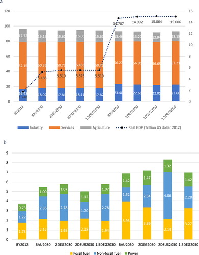
BAU scenario projections allow estimating the 2030 annual investment in energy supply at 174 billion USD i.e. twice the level of recent years (IEA, 2015). The 2DEG scenario would require a 3% increase of that effort (Table 5). The 1.5DEG requires a very similar increase, which reflects that the decrease of energy demand and the increase of unit costs that it prompts broadly compensate one another. The numbers translate to 99.5 billion 2012 USD/year investment in energy supply 2012–2030 for 2DEG scenario, which is close to the number for energy investment by McCollum et al. (2018). In 2050, the additional investment requirement of the 2DEG scenario increases to 15%, which points at the increased cost of clean energy in later years. Again, the 1.5DEG scenario has lower investment requirements thanks to decreasing demand compensating more than the increasing unit costs. The 2DSUS scenario stands apart for its peculiar investment profile. In early years, the anticipation of the 2050 ban on coal power prompts a larger development of cheap coal-fired power and the investment requirements drop 19% compared to BAU. However, in later years, the coal constraint raises investment requirements by 16%. The investment required in energy supply from 2012 to 2050 in the 2DEG scenario amounts to 131.6 billion USD/year while McCollum et al. (2018) reports 210 billion USD/year in 2°C high probability scenario.

Table 5. Energy supply investment at projected horizons.

In billion 2012 USD	Energy supply investment	Variation from BAU
BAU 2030	174.01
2DEG 2030	179.22	3%
2DSUS 2030	141.74	−19%
1.5DEG 2030	179.07	3%
BAU 2050	238.19
2DEG 2050	274.68	15%
2DSUS 2050	276.23	16%
1.5DEG 2050	254.77	7%

Conclusions

The objective of our study was to assess the macroeconomic implications of low carbon development pathways in India. We used a novel methodology of converging bottom-up (AIM/Enduse) and top-down (IMACLIM-IND) models for this purpose. Economy-wide and energy systems implications for India have hardly been assessed by linking national bottom-up and top-down models. Our work makes an important contribution to the existing literature on Indian pathways. We now derive policy-relevant insights from our results which could be useful for decision makers.

Our macroeconomic analysis of India’s pathways to 2030 and 2050 across four scenarios BAU, 2°C, 2°C sustainable and 1.5°C delivers the following results. We find the impact on economic growth of tightening decarbonization targets to be slightly positive, under condition of a maintained investment effort. We also find that decarbonization has a strong bearing on India’s foreign debt via reduced energy trade deficits. Even a stringent 1.5DEG scenario with India’s carbon budget cut by two-thirds compared to BAU results in a slightly higher GDP and a foreign debt contained at 102% of GDP in 2030 and 122% of GDP in 2050. This partly reflects the balance of mitigation costs and energy savings as depicted by our AIM/Enduse model of Indian energy systems. It also stems from the specific Indian energy-economy context, where fossil fuel imports mobilize a substantial share of GDP. Shifting away from fossil fuel based energy systems results in foreign exchange savings of 1 trillion USD from just oil imports over 2012 to 2050. Low-carbon scenarios would thus provide the co-benefit of energy security, as reliance on energy imports reduces thanks to the combined penetrations of domestic non-fossil fuel energy sources and energy efficiency technological innovations. The trade-off here is meeting the higher capital cost to reach the energy intensity targets and avoid locking in capital in inefficient technologies early on. The investment requirements in low carbon scenarios increase compared to the BAU scenario as a result of the shift towards clean technologies. Our results indicate that an energy supply investment of 131 billion USD/year would be required from 2012 to 2050 to achieve low carbon energy systems.

Low-carbon scenarios also raise the share of energy sectors in gross value-added. Further structural transformation in energy systems for low carbon growth is required with renewables constituting a major share of energy consumption, reduced energy demand from industries, commercial sector and households, and employment of clean coal technologies. The nature of those adjustments to the AIM model that allow striking a 1.5°C scenario at little macro-economic cost demonstrates that policymakers can focus on improving energy efficiency and reducing end-use demand. The energy sector transformation might engender conflicts between the entrenched players in the fossil fuel sector and the emerging non-fossil fuel based technology businesses. Policymakers need to balance the interests of both the parties by providing necessary support to both.

In conclusion, low carbon growth is contingent on the availability of transformative technologies and the necessary capital for deploying them. In a developing country like India, where compelling development needs have to be balanced with mitigation targets, international finance may play a vital role in achieving low-carbon development.

Acknowledgements

The IMACLIM model benefits from support of the Chair Long-term Modelling for Sustainable Development (Ponts Paristech-Mines Paristech) funded by Ademe, Grt-Gaz, Schneider Electric, EDF, RTE, Total and the French ministry of Environment. We acknowledge the valuable comments of 3 anonymous reviewers and Dr Depledge. All shortcomings of this paper remain of course our own.

Disclosure statement

No potential conflict of interest was reported by the authors.

Correction Statement

This article has been republished with minor changes. These changes do not impact the academic content of the article.

Additional information

Funding

This research was partially funded by European Union Horizon 2020 research and innovation programme under grant agreement No 642147 (CD-LINKS).

Notes

1 Coupling IMACLIM to AIM/Enduse therefore implies mixing intertemporal optimization of energy investment decisions with simulation of non-energy investment decisions. We consider this a minor, acceptable inconsistency because of the uncertainty surrounding the optimization parameters of AIM/Enduse and conversely, the possibility to describe the exogenous investment decision of IMACLIM as resulting from intertemporal optimization by selecting appropriate parameters. The latter is particularly true in the case of our IMACLIM-IND implementation in single time-steps to 2030 and 2050 horizons.

2 Calibrating the accumulation rule would require settling on ad hoc assumptions regarding the base-year capital stock, the depreciation rate and the pace of investment increase between the base year and projection horizon, to produce ‘sensible’ capital stock estimates (estimates broadly in line with real GDP growth) at projection years. Our way of bypassing the accumulation rule implies that IMACLIM-IND performs comparative statics rather than dynamic recursive analyses, although not at one single year but between two distant years.

3 All our mitigation scenarios thus develop under constraint of global climate action leading to above-2°C warming with high probability. Considering global action increasing in parallel to Indian action would induce considering depressed fossil energy import prices, which would further reduce the costs (or increase the benefits) of the scenarios, although marginally increasing Indian emissions.

4 Additionally, IMACLIM-IND has no way to mark the higher costs of the more efficient equipment ascribed by AIM/Enduse to more ambitious scenarios. This means that identical consumption levels in scenarios with higher mitigation ambitions may mask lower welfare.

Appendices

Appendix A Data hybridization

The data hybridization process outlined below is the first step towards building an original Energy-Environment-Economy (EEE) modelling capacity for determining Indian mitigation pathways. The goal is to reconcile the energy balance and national accounting statistics to produce a dual accounting of energy flows, in volume and money metrics, using agent specific pricing of homogeneous energy goods. This is one of the salient improvements over standard computable general equilibrium techniques where all agents are assumed to buy homogenous energy goods at same net-of-tax price. The process is based on two guiding principles for maintaining consistency of data. First, both physical and money values should follow the conservation principle that is resources and uses must be balanced. Second, the physical and money flows are linked by a unique system of prices implying that the money values can be obtained by multiplying the volumes by the corresponding price. Further, there are two rules guiding the methodology: one, the economic size is always preserved while correcting the statistical gaps; second, the purchasing price heterogeneities faced by different sectors and households is taken into account.

The methodology followed to create the hybrid table has been documented in Combet et al. (2014). It unfolds in three main steps:

1. Reorganizing the original energy balance data (in kilo tons of oil equivalent, Ktoe) and energy prices (in Lakh rupees/ktoe) into the sectoral distribution matching the input-output table (IOT) from national accounting. This not only involves reallocation of physical energy flows of energy balance to production sectors and households, but also entails re-interpretation of the flows in national accounting terms. In other words, it involves sorting out the flows that indeed correspond to economic transaction between national accounting agents. For instance, attributing the autoproduction of electricity to the accounting sectors; considering only the commercial flows especially in case of energy industry own use in energy balance; adjusting the data on international bunkers since energy balance reports data based on geography while IOT reports data based on national accounting rules.

2. Multiplying the volumes with corresponding prices to obtain energy expenses at the same level of disaggregation as IOT.

3. Plugging of the matrix of energy expenditures into original IOT and adjusting the other values of the table such that accounting approach is not disturbed and the total value added of domestic production remains same. This is done by: first, adjusting difference in uses and corresponding resources for energy sectors to the non-energy expenses on pro rata basis; second, by adjusting the difference in original and recomputed expenditures for the non-energy sectors to the most aggregated non-energy good which is ‘other services’ mostly.

Each of these steps must be adapted to the specifics of the energy systems of the region chosen for analysis. It is the purpose of this note to describe how we adapted them in the case of India.

We constructed the commodity × commodity Input Output (IO) table for 65 commodities using the supply and use tables for the year 2012–13 recently released by the Central Statistical Office (CSO), the government organization responsible for coordinating statistical activities in the country. The IO table was constructed by manipulating the supply use matrix, with 140 products and 66 sectors (CSO, 2016), based on industry technology assumption. The data on energy volumes was taken from IEA and AIM/Enduse model. Several government reports and company websites were referred for the data on heterogeneous prices for energy goods.

The decision regarding energy and non-energy sectors was taken based on the specific features of Indian energy sectors and Indian economy. For instance, we take cement and aluminium manufacturing sectors since these are the two most energy intensive sectors in the Indian economy. Government of India (GOI) has specified these sectors as the focus areas for meeting the energy efficiency targets for instance in the policy named Perform Achieve Trade (PAT) scheme. The further decision to add the renewable sector was based on the policy framework being pursued by GOI wherein the target has been set to achieve 175 GW renewable energy capacity by the year 2022. We have taken the 22 products (see Table 1) for the hybridization procedure.

Some notable aspects of Indian energy systems discovered in the hybridization process and their treatment are described below.

• The coal expenses going into electricity sector in original IO were just 25% of those obtained by multiplying available price and volume estimates (hereafter the ‘volume × price’ approach). The official documentation on IO reveals that the coal expenses have been calculated using the inputs of electricity distribution companies like state electricity boards, departmental commercial undertakings of central and state governments and private electricity companies. On the other hand, the volumes in energy balance have been computed using the coal controller’s reports which give the numbers for the output of coal companies going into electricity generation sector. Literature shows that thermal efficiency of coal plants in India is 30% on average (Colin, 2015). This accounts for possible explanation for the mismatch in coal expenses. The remaining differences can be attributed to the fact that several companies like Adani, Tata, Reliance and BHEL generate electricity as a secondary output. Further coal companies like Neyveli Lignite corporation (NLC) are also generating electricity. Due to the above factors, we take the expenses obtained from volume × price rather than those from national accounting IO table.

• Another source of difference in IO and volume × price coal expenses is the phenomenon of captive coal mining (introduced in the year 1993) implying that coal is being produced by sectors like power, iron and steel and cement for their own use. The purpose of the government in allowing private companies into coal mining is to boost the thermal power generation in order to meet the increasing power demand. Though the percentage of captive coal (12%) is not significant compared to total coal produced, it is expected to gain significance in future (Coal Controller’s Organisation, 2015). In order to treat the goods properly, the costs of captive coal mining must be transferred to the coal sector, which is actually the sum of coal mining activities regardless of which sector undertakes the activity. The process involves following steps: (1) the coal expense of captive mines operators is increased via a price × volume approach using the appropriate coal cost net of profit as the price; (2) all cost elements of the coal mining ‘sector’ (activity) are increased homothetically in order to rebalance rise in sales; (3) the costs of the captive mine operator for each item are reduced such as to exactly compensate the cost increase in the coal mining activity. The broad idea is to transfer the costs of the captive coal mining to the general coal mining activity, and to treat captive coal expenses as any other coal expenses. The question of an increase of the share of captive mining in coal expenses can be taken care while modelling pathways by assuming a decrease of the average profit rate of coal mining.

• Next is the trading issue that is natural gas being bought by the refined petroleum sector to be sold to consumers. The refined petroleum products expenses going into chemical and electricity sector from original IO is 2 and 1.5 times respectively of the expenses obtained by volume × price approach. On the other hand, natural gas expenses (original IO) into electricity sector is just 0.3% of the expenses from other approach. Natural gas expenses into chemical sector (original IO) are 37% of those obtained from volume × price approach. Refined petroleum products sector appears to play a role of trader, buying a huge amount of natural gas and selling it back to other businesses without consuming it. This implies that the switch from an industry × industry to a commodity × commodity matrix is not complete, there remains some natural gas sales covered by the refined pet products ‘sector’ of the commodity × commodity matrix. In such a case IO values can be misleading, hence we decide to use volume × price data.

• Bulk of the total energy consumption by households in India is for cooking purpose. Biomass such as firewood, cowdung and agricultural residues, which are normally collected by the households themselves (Pachauri, 2007) is the most commonly used fuel for this purpose. The data on household expenditure on biomass is obtained from the National Sample Survey Office (NSSO), which conducts regular socio-economic survey. Though we have an estimate of the monthly per capita expense on firewood and cow-dung and percentage of people using these fuels, it is hard to get an estimate for the non-market consumption that is number of people collecting the biomass themselves. We compare the household expenses on forestry products specified in IO table (1.3% of total household expenditure) with the firewood and cowdung (1.83% and 0.16% of total household expenditure) consumption from NSSO data. The two numbers seem compatible considering the fact that some proportion of biomass is non-marketable. Hence, we decide to take IOT household expense on forestry sector for representing household expenditure on biomass in the final hybrid matrix.

• Another noteworthy issue was the fact that there are significant amount of non-energy uses of some petroleum products like petroleum coke, lubricants, naphtha and other non-specified oil products in India as opposed to the situation in developed economies. While bitumen non-energy uses were adjusted in the construction sector, petroleum coke was adjusted in cement sector since it is one of the largest consumers of petroleum coke in India. Remaining petroleum coke and other non-energy uses of petroleum products were distributed on pro-rata basis of the respected unaccounted share in volume × price compared to IO expense across all sectors.

Considering the increasing prominence of renewables in the Indian energy policies and the specific tariffs and incentives for this sector, it was added as a separate sector in the matrix. The costs into renewables sector were assumed proportional to the electricity costs after deducting the fossil fuel costs. This assumption is taken for lack of more data on the cost structure. The uses of renewables were calculated based on the feed-in tariff provided by the government and the volumes from the energy balance data.

Appendix B Sensitivity analysis

We conduct sensitivity analysis of our key macroeconomic results to check their variations with changes in exogenous parameters shaping foreign trade flows and household consumption.

Price elasticities of imports and exports have little impact on economic activity measured by real GDP (Tables B1 and B2). The reason is our choice of Johansen closure, which warrants maintained investment effort trajectories (as GDP shares) in all scenarios. Domestic savings thus mechanically compensate the fluctuations of foreign savings mirroring those of the trade balance. Household consumption therefore fluctuates exactly opposite to the trade balance, which improves under lower elasticities and deteriorates under higher elasticities, considering the appreciation of terms-of-trade in all scenarios at both horizons for our central parameterization. The slight GDP adjustments only reflect relative variations of the investment price index and the GDP price index. The trade balance fluctuations induce significant fluctuations of the foreign debt, however not differentiated enough to question our qualitative result of the 2DEG scenario significantly improving the Indian economy’s external position.

Table B1. Sensitivity to price-elasticities of exports (11 goods).

	BAU2050		2DEG2050
	Lower elasticities (x0.9)	Higher elasticities (x1.1)	Lower elasticities (x0.9)	Higher elasticities (x1.1)
Real GDP	+0.001%	+0.001%	−0.001%	0.003%
Hhold consumption (GDP share)	−0.20 pts	+0.20 pts	−0.25 pts	+0.24 pts
Trade balance (GDP share)	+0.20 pts	−0.20 pts	+0.25 pts	−0.24 pts
Foreign debt (ratio to GDP)	−8.76 pts	+8.70 pts	−10.89 pts	+10.70 pts
E imports (GDP share)	+0.01 pts	−0.01 pts	+0.01 pts	+0.00 pts
E exports (GDP share)	+0.002 pts	−0.002 pts	+0.002 pts	−0.001 pts

Table B2. Sensitivity to price-elasticities of imports (11 goods).

	BAU2050		2DEG2050
	Lower elasticities (x0.9)	Higher elasticities (x1.1)	Lower elasticities (x0.9)	Higher elasticities (x1.1)
Real GDP	−0.13%	+0.13%	−0.13%	+0.12%
Hhold consumption (GDP share)	−0.53 pts	+0.52 pts	−0.70 pts	+0.71 pts
Trade balance (GDP share)	+0.53 pts	−0.52 pts	+0.70 pts	−0.71 pts
Foreign debt (ratio to GDP)	−23.39 pts	+23.01 pts	−31.20 pts	+31.46 pts
E imports (GDP share)	−0.002 pts	−0.001 pts	+0.01 pts	−0.01 pts
E exports (GDP share)	−0.02 pts	+0.02 pts	−0.02 pts	+0.02 pts

Conversely, not only the foreign debt but also GDP appear sensitive to variations of the income elasticities that shape household demand of 7 out of the 22 goods of our model, despite the Johansen closure (Table B3). This is because these income-elasticity changes induce structural change via significant shifts of households’ consumption budgets. The ‘Other services’ sector, which captures close to 100% of the budget allocated to non-energy goods without income-elastic specification, has a comparatively high labour efficiency. Structural change in its favour via lower income-elasticities of the 7 income-elastic goods significantly improves real GDP, and conversely.

The impact on the foreign debt via that on the cumulated trade deficits is massive. In the case of the BAU, higher income-elasticities i.e. a lesser structural change in favour of labour-extensive services leads India towards an unsustainable foreign debt above 300% (204.9% + 104.1%) of its GDP in 2050. This could not but induce macroeconomic shocks outside the scope of our modelling tool. The 2DEG scenario mitigates this risk but still see the debt overcome 220% (133.0%+91.0%) of GDP in 2050 in case of lesser structural change.

Table B3. Sensitivity to income-elasticities of household consumptions (7 goods).

	BAU2050		2DEG2050
	Lower elasticities (x0.9)	Higher elasticities (x1.1)	Lower elasticities (x0.9)	Higher elasticities (x1.1)
Real GDP	+8.41%	−7.42%	+8.15%	−7.34%
Hhold consumption (GDP share)	−1.67 pts	+2.28 pts	−1.47 pts	+2.00 pts
Trade balance (GDP share)	+1.67 pts	−2.28 pts	+1.47 pts	−2.00 pts
Foreign debt (ratio to GDP)	−76.28 pts	+104.10 pts	−67.11 pts	+91.04 pts
E imports (GDP share)	−0.77 pts	+1.11 pts	−0.58 pts	+0.82 pts
E exports (GDP share)	−0.32 pts	+0.44 pts	−0.30 pts	+0.38 pts

Appendix C Scenario implementation

Table C1. Scenario policies, corresponding AIM/Enduse drivers/constraints, results and insights.

Sector	Policy	Policy Instruments/mechanism	AIM/Enduse driver/ constraint	Result	Key Insights
Electricity	Increase non-fossil capacity to 175 GW	Solar: 100 GW, Wind: 60 GW, Small hydro: 15 GW, Biomass: 25 GW by 2030	Capacity targets (BAU: 250 GW by 2050, 2DEG: 400 GW by 2050, 2DSUS: 500 GW by 2050)	Increase in non-fossil capacity	Fossil-based capacity reduces, improvement in thermal and electricity efficiency, lower AT&C losses are main contributors for GHG emission reduction.
	National Solar Mission (NSM)	Regulation: Solar Target – 100 GW by 2030	Capacity target (BAU: 180 GW by 2050, 2DEG: 220 GW by 2050, 2DSUS: 250 GW by 2050)
	National Mission on Enhanced Energy Efficiency (NMEEE)	Market Instrument: Perform, Achieve and Trade (PAT)	Gradual improvement of energy-efficiency for 10 types of electric appliances^a	Improve EE (Energy Efficiency) in old coal plants
	National Mission for clean coal technologies	Phase out of conventional coal power, addition of fuel-efficient generation options (PC, IGCC, SC and USCC)	Promoting efficient technology (up to 110 GW of super-critical in NDC and 2DEG by 2050), retirement of older (>25 years) plants that have lower efficiency than PAT targets	Phase-out of old, inefficient coal technologies, Installation of supercritical thermal power stations, development of ultra-super critical technology, CCS
	Improving the National Power Grid	Strengthening transmission and distribution power systems, more efficient load dispatch	Reduction of transmission and distribution losses, range 0.25-0.5 percentage point/year until the national average aggregate technical and commercial (AT&C) losses reach 15% from current 22%	Reduction in transmission and distribution losses
Industry	National Mission on Enhanced Energy Efficiency (NMEEE)	Market Instrument: Perform, Achieve and Trade (PAT). Including new designated consumers (DCs) under PAT. Recycling of material, waste heat recovery	Improvement of specific energy consumption for 11 sectors^b	Energy saving potential increase; process improvement; increased recycling	Reduction in energy consumption in energy intensive industries
Transport	National Urban Transport Policy, National Mission on Sustainable Habitat Mission, National Electric Mobility Mission Plan (NEMMP) 2020 National biofuel policy	Passenger: Ethanol blending- 5%, Increase in electric vehicles (EV), increase in public transport	Adjustment of modal demands, Adjustment of allowable service share by EV	Increase in non-motorized transport; rail and mass rapid transit; Increase in electric vehicles technology – rise in biofuels blending	Petrol and diesel consumptions reduce, increase in electricity consumption
		Freight: Service share increase in transport demand from 36 to 45% through dedicated freight corridor (DFC) by 2050, improve vehicle efficiency	Adjustment of freight modal demand, Adjustment of allowable service share by rail	Increase in rail transport
Residential and Commercial Sectors	NSM, NMEEE, NSHM	Energy-efficient residential and commercial through Energy Conservation Building Code (ECBC); Standards and Labelling (S&L) Programme, UJALA and UJJWALA schemes^c	Introduced efficient technologies in each enduses in these sectors (selection based on cost optimization)	Replacement of firewood stoves with LPG and solar technologies; shift to solar heating systems, phase-out of incandescent lights, kerosene lamps and shift to LEDs; Increase in EE appliances like refrigerators, air conditioners; EE buildings	Shift from biomass to cleaner forms of energy (LPG, electric, PNG), higher penetration of energy efficient technologies
Agriculture	NSM, NMEEE	Shift to solar pumps (phased), increased use of EE pumps	Reducing energy consumption per 1000 litres water pumping through EE pumps	Technology improvement in diesel and electric pumps, tractors	Less fossil fuel consumption

^aFor air conditioners, refrigerators, distribution transformers, tubular fluorescent lights, ceiling fans, TVs, refrigerators, washing machines, gas stoves, water pump sets (Garg, Dhar, Kankal, & Mohan, 2017).

^bAluminium, cement, chlor-alkali, fertilizer, iron & steel, paper & pulp, thermal power plant, textile, railways, electricity DISCOMS (distribution companies) and refineries (in all 737 DCs under PAT)

^c770 million LED bulbs to domestic consumers (UJALA programme); 80 million beneficiaries (Ujjwala scheme).

Appendix D Soft-linking convergence process

In the Tables D1–D5 below we provide the values of energy-economy variables in the pre-iterations and post-iterations stages of IMACLIM-IND and AIM/Enduse coupling process. The rationale behind the coupling of bottom-up and top-down models is investigated in Hourcade et al. (2006) and Ghersi (2015). This approach benefits from the strengths (and avoids the weaknesses) of both models.

Table D1. Aggregate energy consumption mix of productive sectors pre and post iterations.

	BAU2050		1.5DEG2050
	Pre iterations (%)	Post iterations (%)	Pre iterations (%)	Post iterations (%)
COAL	27.81	28.96	24.99	22.43
COKE	9.16	6.89	8.37	6.29
OILNTFUEL	18.95	12.54	18.74	12.05
TRANSPFUEL	8.64	14.70	11.28	19.96
BIOMASS	1.59	2.15	1.54	2.31
NATURALGAS	13.00	10.29	13.68	10.11
ELECTRICITY	20.56	22.68	21.18	25.33
RENEWABLE	0.28	1.78	0.23	1.52

Table D2. Macroeconomic results pre and post iterations.

	BAU2050		1.5DEG2050
	Pre iterations	Post iterations	Pre iterations	Post iterations
Real GDP (Trillion US dollar 2012)	17.64	14.71	17.19	15.01
Average annual real GDP growth (%)	6.28%	6.26%	6.21%	5.83%
Household consumption, GDP share	63.32%	66.44%	65.44%	64.59%
Trade balance, GDP share	−4.87%	−7.99%	−6.99%	−6.14%
CPI	1.35	1.23	1.45	1.29
E imports, GDP share	5.98%	7.34%	7.17%	5.04%
E expenses, GDP share	19.05%	26.95%	13.03%	25.42%
E exports, GDP share	1.58%	2.28%	1.22%	2.15%
REER	1.05	1.05	1.11	1.11

Table D3. Power generation mix pre and post iterations.

	BAU2050		1.5DEG2050
	Pre iterations (%)	Post iterations (%)	Pre iterations (%)	Post iterations (%)
COAL	27.56	31.63	27.19	22.51
COKE	0.00	0.00	0.00	0.00
OILNTFUEL	1.20	1.16	2.15	1.37
TRANSPFUEL	0.00	0.00	0.00	0.00
BIOMASS	13.24	13.61	11.59	11.17
NATURALGAS	50.37	38.04	40.28	33.25
ELECTRICITY	0.00	0.00	0.00	0.00
RENEWABLE	7.64	15.55	18.79	31.69

Table D4. Household energy consumption mix pre and post iterations.

	BAU2050		1.5DEG2050
	Pre iterations (%)	Post iterations (%)	Pre iterations (%)	Post iterations (%)
COAL	0.00	0.00	0.00	0.00
COKE	0.00	0.00	0.00	0.00
OILNTFUEL	12.88	30.59	15.01	31.89
TRANSPFUEL	35.73	19.50	3.93	1.43
BIOMASS	6.39	14.22	9.63	18.32
NATURALGAS	0.20	0.11	0.00	0.00
ELECTRICITY	32.64	16.66	55.43	24.71
RENEWABLE	12.16	18.92	16.00	23.64

Table D5. Shares of industrial sectors in total output pre and post iterations.

	BAU2050		1.5DEG2050
	Pre iterations (%)	Post iterations (%)	Pre iterations (%)	Post iterations (%)
IRONSTEEL	2.31	2.54	2.32	2.55
CHEMPETROCHEM	2.80	2.50	2.82	2.35
ALUMINIUM	0.74	0.92	0.75	0.90
CEMENT	1.18	1.08	1.20	1.12
CONSTRUCTION	10.55	9.19	10.68	9.57
TEXTILE	1.95	2.79	1.98	2.79
RESIDINDUSTRIES	13.87	17.01	13.98	16.78

References

- Blanchflower, D. G., & Oswald, A. J. (2005). The wage curve reloaded. Working Paper 11338. Cambridge, MA: National Bureau of Economic Research, 46 p.
- Byravan, S., Ali, M. S., Ananthakumar, M. R., Goyal, N., Kanudia, A., Ramamurthi, P. V., … Paladugula, A. L. (2017). Quality of life for all: A sustainable development framework for India’s climate policy reduces greenhouse gas emissions. Energy for Sustainable Development, 39, 48–58. doi: https://doi.org/10.1016/j.esd.2017.04.003
- CD-Links. (2019). The global stocktake: Keeping track of implementing the Paris agreement. Retrieved from https://themasites.pbl.nl/global-stocktake-indicators/
- Chaturvedi, V., Koti, P. N., & Chordia, A. R. (2018). Pathways towards nationally determined contribution and mid-century strategy. New Delhi: Council on Energy, Environment and Water (CEEW).
- Coal Controller’s Organisation. (2015). Coal directory of India 2013-2014. Coal statistics. Government of India. Ministry of Coal. Kolkata: Coal Controller’s Organisation. Retrieved from https://www.coal.nic.in/sites/upload_files/coal/files/curentnotices/coaldir13-14_0.pdf
- Colin, H. (2015). Coal fired power plant efficiency improvement in India. London: IEA Clean Coal Center.
- Combet, E., Ghersi, F., Lefèvre, J., & Le Treut, G. (2014). Construction of hybrid input-output tables for E3 CGE model calibration and consequences on energy policy analysis. Global Trade Analysis Project. West Lafayette, IN: Purdue University. Retrieved from https://www.gtap.agecon.purdue.edu/resources/res_display.asp?RecordID=4524
- CSO. (2016). Supply and use table, a note on compilation for the years 2011-12 and 2012-13. New Delhi: Central Statistics Office, Ministry of Statistics and Programme Implementation. Retrieved from http://mospi.nic.in/sites/default/files/reports_and_publication/statistical_publication/National_Accounts/SUT_Methodology_final_noteforwebsite.pdf
- Dhar, S., Pathak, M., & Shukla, P. R. (2018). Transformation of India’s transport sector under global warming of 2°C and 1.5°C scenario. Journal of Cleaner Production, 172, 417–427. doi: https://doi.org/10.1016/j.jclepro.2017.10.076
- Dubash, N. K., Khosla, R., Rao, N. D., & Sharma, K. R. (2015). Informing India’s energy and climate debate: Policy lessons from modelling studies. New Delhi: Centre for Policy Research.
- Economic Survey. (2018). Economic survey 2017–18. Government of India. Ministry of Finance. Department of Economic Affairs. Economic Division. Retrieved from http://mofapp.nic.in:8080/economicsurvey/
- ETEnergyWorld. (2018). India’s monthly oil import bill growth at a year-high. Retrieved from https://energy.economictimes.indiatimes.com/news/oil-and-gas/indias-monthly-oil-import-bill-growth-at-a-year-high/63015213
- Fortes, P., Simões, S., Seixas, J., Van Regemorter, D., & Ferreira, F. (2013). Top-down and bottom-up modelling to support low-carbon scenarios: Climate policy implications. Climate Policy, 13(3), 285–304. doi: https://doi.org/10.1080/14693062.2013.768919
- Fragkos, P., Fragkiadakis, K., Paroussos, L., Pierfederici, R., Vishwanathan, S. S., Köberle, A. C., … Oshiro, K. (2018). Coupling national and global models to explore policy impacts of NDCs. Energy Policy, 118, 462–473. doi: https://doi.org/10.1016/j.enpol.2018.04.002
- Fragkos, P., & Kouvaritakis, N. (2018). Model-based analysis of intended nationally determined contributions and 2°C pathways for major economies. Energy, 160, 965–978. doi: https://doi.org/10.1016/j.energy.2018.07.030
- Gambhir, A., Napp, T. A., Emmott, C. J., & Anandarajah, G. (2014). India’s CO2 emissions pathways to 2050: Energy system, economic and fossil fuel impacts with and without carbon permit trading. Energy, 77, 791–801. doi: https://doi.org/10.1016/j.energy.2014.09.055
- Garg, A., Dhar, S., Kankal, B., & Mohan, P. (2017). Good practice and success stories on energy efficiency in India. Retrieved from http://orbit.dtu.dk/files/140952224/GOOD_PRACTICE_INDIA_WEB_Version.pdf
- Ghersi, F. (2015). Hybrid bottom-up/top-down energy and economy outlooks: A review of IMACLIM-S experiments. Frontiers in Environmental Science, 3, 74. doi: https://doi.org/10.3389/fenvs.2015.00074
- Grubb, M., Edmonds, J., ten Brink, P., & Morrison, M. (1993). The costs of limiting fossil-fuel CO2 emissions: A survey and analysis. Annual Review of Energy and the Environment, 18(1), 397–478. doi: https://doi.org/10.1146/annurev.eg.18.110193.002145
- Gupta, D., Ghersi, F., & Garg, A. (2018a). Hybrid input-output tables for India at year 2012, Mendeley Data, v2. Retrieved from https://data.mendeley.com/datasets/d7ffryvtjk/2
- Gupta, D., Ghersi, F., & Garg, A. (2018b). The IMACLIM-India model version 1.0. CIRED working paper 2018–71. Paris: CIRED. Retrieved from http://www2.centre-cired.fr/IMG/pdf/cired_wp_2018_71_ghersi.pdf
- Hourcade, J.-C., Jaccard, M., Bataille, C., Ghersi F. (2006). Hybrid modelling: New answers to old challenges. The Energy Journal, special issue Hybrid Modelling of Energy-Environment Policies: Reconciling Bottom-Up and Top-Down, 1–12.
- IEA. (2015). World energy outlook 2015. Paris: International Energy Agency.
- IEA. (2018). World energy outlook 2018. Paris: International Energy Agency.
- Kainuma, M., Matsuoka, Y., & Morita, T. (Eds.). (2011). Climate policy assessment: Asia-Pacific integrated modeling. Tokyo: Springer Science & Business Media.
- Krook-Riekkola, A., Berg, C., Ahlgren, E. O., & Söderholm, P. (2017). Challenges in top-down and bottom-up soft-linking: Lessons from linking a Swedish energy system model with a CGE model. Energy, 141, 803–817. doi: https://doi.org/10.1016/j.energy.2017.09.107
- Le Treut, G. (2017). Methodological proposals for hybrid modelling: Consequences for climate policy analysis in an open economy. Doctoral dissertation. France: École Doctorale Ville, Transports et Territoires (VTT)-ED 528. Retrieved from https://hal.archives-ouvertes.fr/tel-01707559/
- McCollum, D. L., Zhou, W., Bertram, C., De Boer, H. S., Bosetti, V., Busch, S., … Fricko, O. (2018). Energy investment needs for fulfilling the Paris agreement and achieving the sustainable development goals. Nature Energy, 3(7), 589–599. doi: https://doi.org/10.1038/s41560-018-0179-z
- Mittal, S., Liu, J. Y., Fujimori, S., & Shukla, P. (2018). An assessment of near-to-mid-term economic impacts and energy transitions under “2° C” and “1.5° C” scenarios for India. Energies, 11(9), 2213. doi: https://doi.org/10.3390/en11092213
- MoEFCC. (2015). India’s intended nationally determined contribution: Working towards climate justice. Ministry of Environment, Forests and Climate Change, Government of India. Retrieved from http://www4.unfccc.int/ndcregistry/PublishedDocuments/India%20First/INDIA%20INDC%20TO%20UNFCCC.pdf
- MoSPI. (2018). India in figures 2018. Government of India. Ministry of statistics and Programme Implementation. Central Statistics Office. Retrieved from http://mospi.nic.in/sites/default/files/publication_reports/India_in_figures-2018_rev.pdf
- NEP. (2017). Draft national energy policy. NITI Aayog, Government of India. Version as on 27.06.2017. Retrieved from http://niti.gov.in/writereaddata/files/new_initiatives/NEP-ID_27.06.2017.pdf
- Pachauri, S. (2007). An energy analysis of household consumption (Vol. 13). Dordrecht: Springer Science & Business Media.
- Parikh, J., & Parikh, K. (2011). India’s energy needs and low carbon options. Energy, 36(6), 3650–3658. doi: https://doi.org/10.1016/j.energy.2011.01.046
- PMCoCC. (2008). National action plan on climate change. Government of India. Prime Minister’s Council on Climate Change. Retrieved from http://www.moef.nic.in/downloads/home/Pg01-52.pdf
- Pradhan, B. K., & Ghosh, J. (2012). The impact of carbon taxes on growth emissions and welfare in India: A CGE analysis. Institute of Economic Growth Working Paper No. 315. Retrieved from http://www.iegindia.org/upload/publication/Workpap/wp315.pdf
- Saveyn, B., Paroussos, L., & Ciscar, J. C. (2012). Economic analysis of a low carbon path to 2050: A case for China, India and Japan. Energy Economics, 34, S451–S458. doi: https://doi.org/10.1016/j.eneco.2012.04.010
- SECC. (2015). Socio economic and caste census 2011. Released in 2015. Retrieved from http://secc.gov.in
- Sen, A. K. (1963). Neo-classical and Neo-Keynesian theories of distribution. Economic Record, 39(85), 53–64. doi: https://doi.org/10.1111/j.1475-4932.1963.tb01459.x
- Shukla, P. R., & Chaturvedi, V. (2012). Low carbon and clean energy scenarios for India: Analysis of targets approach. Energy Economics, 34, S487–S495. doi: https://doi.org/10.1016/j.eneco.2012.05.002
- Shukla, P. R., Dhar, S., & Mahapatra, D. (2008). Low-carbon society scenarios for India. Climate Policy, 8(sup1), S156–S176. doi: https://doi.org/10.3763/cpol.2007.0498
- Tavoni, M., Kriegler, E., Riahi, K., van Vuuren, D., Petermann, N., Jewell, J., … Rosler, H. (2014). Limiting global warming to 2 degree C – Policy findings from Durban platform scenario analyses. Low climate impact scenarios and the implications of required tight emission control strategies project. Retrieved from website: http://services.feem.it/userfiles/attach/20141215160104PB2_9_c.pdf
- van den Berg, N. J., van Soest, H. L., Hof, A. F., den Elzen, M. G., van Vuuren, D. P., Chen, W., … Kõberle, A. C. (2019). Implications of various effort-sharing approaches for national carbon budgets and emission pathways. Climatic Change. doi: https://doi.org/10.1007/s10584-019-02368-y
- Vandyck, T., Keramidas, K., Saveyn, B., Kitous, A., & Vrontisi, Z. (2016). A global stocktake of the Paris pledges: Implications for energy systems and economy. Global Environmental Change, 41, 46–63. doi: https://doi.org/10.1016/j.gloenvcha.2016.08.006
- van Ruijven, B. J., Weitzel, M., den Elzen, M. G., Hof, A. F., van Vuuren, D. P., Peterson, S., & Narita, D. (2012). Emission allowances and mitigation costs of China and India resulting from different effort-sharing approaches. Energy Policy, 46, 116–134. doi: https://doi.org/10.1016/j.enpol.2012.03.042
- Van Soest, H. L., Reis, L. A., Drouet, L., Van Vuuren, D. P., Den Elzen, M. G., Tavoni, M., … Luderer, G. (2017). Low-emission pathways in 11 major economies: Comparison of cost-optimal pathways and Paris climate proposals. Climatic Change, 142(3–4), 491–504. doi: https://doi.org/10.1007/s10584-017-1964-6
- Van Soest, H., Reis, L., van Vuuren, D. P., Bertram, C., Drouet, L., Jewell, J., … Tavoni, M. (2016). Regional low-emission pathways from global models. SSRN Electronic Journal. https://doi.org/10.2139/ssrn.2718125
- Vishwanathan, S. S., Fragkos, P., Fragkiadakis, K., Paroussos, L., & Garg, A. (2019). Energy system transitions and macroeconomic assessment of the Indian building sector. Building Research & Information, 47(1), 38–55. doi: https://doi.org/10.1080/09613218.2018.1516059
- Vishwanathan, S. S., Garg, A., & Tiwari, V. (2018). Coal transition in India. Assessing India’s energy transition options. Paris: IDDRI and Climate Strategies.
- Vishwanathan, S. S., Garg, A., Tiwari, V., Kankal, B., Kapshe, M., & Nag, T. (2017). Enhancing energy efficiency in India: Assessment of sectoral potentials. Copenhagen: Copenhagen Centre on Energy Efficiency, UNEP DTU Partnership.
- Vishwanathan, S. S., Garg, A., Tiwari, V., & Shukla, P. R. (2018). India in 2°C and well below 2°C worlds: Opportunities and challenges. Carbon Management, 9, 459–479. doi: https://doi.org/10.1080/17583004.2018.1476588