Nature to the rescue: past drivers and future potential of the Australian land-based carbon offsets market

ABSTRACT

Large quantities of ‘negative emissions’ will be required to meet the 1.5°C temperature target under the Paris agreement. As nations consider more ambitious emissions reductions goals, policy makers, carbon market participants and environmental advocates need to estimate the potential scale of nature-based climate solutions (NCS), against the opportunity cost of current land use. In this study we construct a simple linear regression model of the relationship between carbon abatement potential and agricultural profitability, the latter a proxy for opportunity cost, to describe the total set of options for NCS on the Australian continent. Sampling these same two variables at the sites of over 800 land-based offset projects accredited since 2015 shows how the market selected from these abatement options. The model demonstrates that offset projects, under a range of crediting methodologies, were typically selected where the ratio of abatement potential to opportunity cost is maximized. These results, produced from two readily available spatial variables, provide an empirically derived framework for those with an interest in the structure of the long-run supply curve for land-based carbon abatement. This modelling approach could be applied in any geographic region where similar spatial variables for agricultural profitability and abatement potential are available.

Key policy insights:

• We find a strong positive correlation between the quantity of abatement potential on a land parcel and its potential opportunity cost, the latter represented by agricultural profitability.

• The lowest cost abatement will be obtained by policies, including market mechanisms, that optimize these two factors rather than prioritizing one over the other.

• Policies that direct projects to ‘marginal’ agricultural land may lead to a more costly emissions reduction pathway.

• Our modelling approach is a key input to the development of a long-run supply curve for land-based abatement, essential to any strategy that relies heavily on negative emissions.

• Understanding the drivers of land-based abatement projects can help to predict the land use policy impacts of a higher offset requirement.

KEYWORDS:

• Nature-based climate solutions
• negative emissions
• offsets

1. Introduction

‘Negative emissions’ will be essential to meet the 1.5°C temperature target under the Paris agreement (Intergovernmental Panel on Climate Change, 2019; Minx et al., 2018). Understanding the available quantity of such options has become critical to global emissions target-setting (Bednar et al., 2019; Fajardy & Mac Dowell, 2017; Fuss et al., 2018; Jackson et al., 2017; Kato & Yamagata, 2014; Minx et al., 2017, 2018). Negative emissions can be achieved through technological solutions (e.g. direct carbon dioxide removal from the atmosphere (Minx et al., 2017)) or from Nature-based climate solutions (NCS), where emissions are avoided or additional carbon is stored in ecological systems.

As nations seek least cost trajectories to net zero emissions, policy makers, market participants and environmental advocates wish to understand the quantity of NCS abatement options available, their likely cost, and their effects on economic, biophysical and social systems (Australian Government, 2021; Carbon Market Institute, 2016, 2017; Climateworks, 2010; Nature4climate, 2019).

Some authors point to the potential for land-use competition from large-scale negative emissions programmes (Benton et al., 2018; Bradshaw et al., 2013; Brown et al., 2019; Seddon et al., 2021; Zomer et al., 2008). Climate change itself is expected to reduce the available arable land (Zhang & Cai, 2011), while the occurrence of conflicts that interrupt food supply, such as the war in Ukraine (Jagtap et al., 2022), are even less predictable.

Well-considered NCS have, and may further offer, social and economic co-benefits (Busch et al., 2019; Dooley et al., 2018; Fargione et al., 2018; Griscom et al., 2020), when contrasted with the untested implications of technologies such as bioenergy with carbon capture and storage (BECCS) (Fajardy & Mac Dowell, 2017; Fridahl and Lehtveer, 2018; Gambhir et al., 2019; Kato & Yamagata, 2014; Pour et al., 2018). However, with a limited land-base and potential conflict with agricultural and forestry uses (Burke, 2021; Keith et al., 2019) NCS options need to be carefully evaluated against other aims of land use policy (Cohen-Shacham et al., 2019; Connor et al., 2016; Hoyos-Santillan et al., 2021). One of the purposes of an emissions market is to optimize the allocative efficiency of this scarce resource (Weishaar, 2007). The operation of a market may also ensure that decentralized ‘knowledge of the particular circumstances of time and place will be promptly used’ (Hayek, 1945). When considering land and ecosystem-based abatement supplied from a multiplicity of individually owned land parcels, owners and managers will vary in their capacities to act and their preferences, yet they are best placed to understand and act on their own economic opportunities. Important local biophysical conditions, which influence abatement potential, may not be visible to continent-wide ecological models but can be discerned and acted upon at the local level.

The aim of this study is to better understand the drivers of the supply of carbon offsets from the Australian landscape, by developing a simple explanatory model (Shmueli, 2010) relating abatement potential to opportunity cost.

An assumption by some advocates has been that carbon sequestration will be accommodated on ‘marginal’ (i.e. low profitability) agricultural land (Climateworks, 2010; Farmers for Climate Action, 2021; Wood et al., 2021). In the Australian government’s plan for achieving net zero emissions by 2050 (Australian Government, 2021), it is stated that abatement of up to 65 Mt CO₂-e per annum can be achieved by planting trees on marginal agricultural land or integrated into farming with minimal loss of production. However, low profitability land may also have low carbon sequestration potential. In fact, some ‘degraded’ lands may be a poor prospect for carbon abatement, as it may be difficult to reverse the processes that caused carbon loss, e.g. if soil profiles are damaged or vegetation seedbanks lost (Chappell & Baldock, 2016; Dean et al., 2015). This study’s approach tests whether directing offset projects to land with low agricultural profitability is likely to be an efficient approach in future.

2. Literature review

A large body of literature has considered the drivers of the supply and cost of emissions mitigation. In this review we focus on the studies most comparable to ours, that is, considering a regional land base rather than an industry sector, focusing on NCS, and observing or simulating an emissions trading system. Approaches include macro-economic and spatial models with feedback, quantifying abatement by method, farm or enterprise level analysis and assessment of other barriers to supply.

Australian offsets are created under baseline and credit methodologies (hereafter, ‘methods’) of abatement which are approved under federal legislation (‘Carbon Credits (Carbon Farming Initiative) Act, 2011 Cth,’) and each project and its credits are recorded on a central register. This market has continued to grow and evolve since its inception in 2015, with 125.6 million tonnes CO₂-e of Australian Carbon Credit Units (ACCUs), registered at the time of publication (Clean Energy Regulator, 2021c), the majority to land-based projects. By comparison, the California Air Resources Board has issued 221 million tonnes CO₂-e of offset credits from forest, livestock, Mine Methane Capture and Ozone Depleting Substances methods (California Air Resources Board, 2021) and the UNFCCC Clean Development Mechanism with over 2 billion tonnes CO₂-e of Certified Emissions Reductions, only records 2.2 million tonnes CO₂-e from afforestation/reafforestation methods and 10.9 million tonnes CO₂-e from agricultural projects (UNFCCC, n.d.).

The total cost of an abatement project will be the cost of project activities and transactions costs, to create and securitize the abatement, plus the opportunity cost of any lost agricultural production. Where carbon abatement projects are in competition with agricultural use of land, or even where they can be integrated within these production systems, the markets for carbon and agricultural commodities may become linked (Connor et al., 2015). Australia’s agricultural land already supplies commodities into competitive, globalized markets (Chang & Griffith, 1998; Dong et al., 2018). Mindful of this issue, academic interest has turned to approaches for estimating the potential of NCS options using an opportunity cost approach.

Inputs to such models may comprise:

• known or estimated cash flows from the existing land use, often as a net present value with a range of discount rates,

• estimates of biodiversity, social, cultural or community benefits, including household consumption of harvested products,

• project costs and transaction costs, and;

• a proposed carbon price or a range of prices, or an emissions reduction goal, applied to total project or time-averaged additional abatement.

A literature review of studies of opportunity cost of reducing deforestation and forest degradation (Yang & Li, 2018) found that the range of values used for discount rate, product price and yield, carbon density and time horizons were the most influential and often varied even amongst different studies of the same activity.

For assessment of NCS potential and cost at the global scale, Integrated Assessment Models (Roe et al., 2021), general equilibrium models (Golub et al., 2009) or country rankings (Grafton et al., 2021) have been deployed. Complex economic optimization models with a spatial component use inputs of carbon prices and outputs of land-based mitigation, for Australia (Bryan et al., 2016; Connor et al., 2015) and the US (Wade et al., 2022). These model abatement along with scenarios for broader economic change, such as changing demand for agricultural commodities. At the global scale, the forest sink was modelled (Daigneault et al., 2022) by estimating the effect of climate policy scenarios on supply of carbon sequestration, timber products and land for agriculture. Climate effects such as wildfire or CO2 fertilization were not modelled.

Beyond the broad national or global surveys which aim to assess the size of NCS options, studies have attempted to develop models of sequestration project land use incorporating opportunity cost at more localized scales (Anh et al., 2016; Anup et al., 2014; Chu & Liu, 2021; Man et al., 2015; Siikamäki & Newbold, 2012; Tomich et al., 2002).

Longmire et al. (2015) approached the question of carbon abatement opportunity cost specifically in the Australian context, although restricted to tree planting methodologies only, and developed a model for revegetation projects on agricultural land. Sequestration potential was obtained from a detailed spatial model of environmental plantation growth known as FullCAM (Richards & Evans, 2004) which is also used in preparing Australia’s National Inventory Report (Australian Government Department of Industry Science Energy and Resources, 2020a). The study used statistical reports on local values of agricultural production in $ ha⁻¹ year⁻¹ to assess opportunity cost at sites representing ten farming systems. Abatement potential was calculated to include avoided emissions from the existing agricultural land use, which was not included in our study, as this aspect is not a feature of current crediting methodologies. These emissions were highest in high rainfall areas with cattle production systems. Comparisons between their ten study areas indicated that it was the combinations of profitability of existing land use with carbon potential that determined optimum financial return, rather than the maximization of any one factor. A similar approach was used at the regional scale for Caterbury, New Zealand (Funk et al., 2014) finding that carbon sequatration capacity, carbon price and expected grazing income influenced the financial outcome. To estimate the opportunity costs of soil carbon projects, Kragt et al. (2012) combined a soil carbon accretion model across a spatial map of soil types, combined with a farm level model of profit maximization, in an Australian cropping zone. Carbon storage was enhanced by increasing the length of the pasture rotation, or crop waste retention however these options also reduced revenue, thus developing a trade-off curve which would vary with prevailing commodity prices. Another spatial model (Ausseil et al., 2019) integrated biophysical and economic variables to understand how IPCC climate and emissions scenarios could drive future land use change for a selected locality in New Zealand. Variables were dynamic over time, including climatic, demographic, and economic (incorporating a carbon price) under the driving scenarios of the IPCC global emissions pathways. An important effect was that carbon prices rose faster than certain meat and milk prices driving a transition to tree plantations.

In a related approach Carroll and Daigneault (2019) included agricultural practices focussing on animal waste management and methane reduction in an economic/land use/emissions model for New Zealand. However, the high or untested costs of these abatement methods meant that achieving the desired targets required multiple methods with costs up to $100/tCO2e. Reforestation thereby became the largest and cheapest source of mitigation. The obvious limitation of these approaches is that estimates for both cost and scale must be programmed in when they have not been widely adopted at this time.

A model (Barry et al., 2014) of the potential for expanded commercial tree growing on less productive farmland in New Zealand used net present value of timber growing, incorporating carbon credits and a range of other environmental benefits, as a measure of land value. The prevailing market price of carbon credits at $NZ4 was used. A pre-existing spatial layer of tree productivity was available as an input. They were able to conclude that without the public benefits, few additional areas would be viable on commercial value alone.

Land valuations, rather than profits were preferred as the explanatory variable in Polglase et al. (2013), on the view that committing to carbon sequestration was a ‘one-way’ decision with loss of option value. However they acknowledged that the alternative uses may themselves have an impact on land values over time and after market responses. Competition for land between agriculture and carbon uses may to lead to increased land values. There has been some research into methods of land valuation using the cash flows from carbon projects (Blake & Eves, 2012; Blake, 2016; Regan et al., 2015).

There have been attempts to estimate the quantities of land-based carbon abatement for Australia (Australian Government, 2021; Climateworks, 2010; Eady et al., 2009; Lawson et al., 2008; McKinsey and Company, 2008; Regan et al., 2019; The Nous Group, 2010). These often examine possible methods and seek to quantify the abatement available from each.

In addition to macro-economic and spatial studies, modelling has also been conducted at the farm or enterprise level. Regan et al. (2020) constructed a theoretical discounted cash flow analysis to assess the economics of reafforestation for South Australia, while Evans ( 2018) and Evans et al. (2015) and Maraseni and Cockfield (2015) similarly examined Queensland and Sinnett et al. (2016) for Victoria. White and Davidson (2016) examined the potential costs and benefits of agricultural soil carbon methods. A farm operation model (Monjardino et al., 2010) was adapted to include forage shrubs, with associated carbon storage, as one of the management options, for the west Australian wheat belt. Such an approach could be valuable in understanding some of the farm-level factors which may not be visible in broad scale spatial model such as ours. Ultimately these studies aim to understand the cost or economic viability of different project methods. However, in our study projects could be said to have passed the test of viability, in that they are already participants in a competitive offset market.

There are additional factors that may impact on supply beyond those variables included in our model. These effects become important to our approach if they have a spatially varying effect. For brevity, we include our literature review of issues related to market design, offset integrity and barriers to participation in the Supplementary Material.

Other modelling approaches have incorporated globally influenced agricultural prices and market fluctuations and produced outputs in the form of estimates of changing land use between different commodities including carbon abatement.

Building on these theoretical and modelling insights, in this study we take advantage of real-world data from the Australian offsets market and take measures of the abatement potential and agricultural profitability of registered Australian offset projects. While our model lacks the time-varying dynamics of some other models, the advantage is that we use as inputs the actual outcomes from the agricultural and carbon market systems and compare these with estimates of abatement potential and its opportunity cost. This will be the first study to examine the whole Australian continent, modelling all currently approved sequestration methods and using real world data from the functioning offsets market.

3. Methods

In our model, the two drivers of offset project selection across the landscape are carbon abatement potential and financial opportunity cost. We expect that from the total set of options for land-based abatement, the offsets market will select projects with the lowest carbon opportunity cost.

We take advantage of newly available spatial data on key variables of maximum above-ground biomass potential (Roxburgh et al., 2019), which can serve as a proxy for emissions abatement available, and annual agricultural land profitability (Marinoni & Navarro Garcia, 2018), as an estimator of profits possibly foregone, that is, opportunity cost.

The two proxy variables are sampled with two groups of spatial points. One group of points are at the location of real-world offset projects. These projects were developed between 2012 and 2021, to compete in offset auctions where the average carbon prices varied from $A10-16. The other group of points were randomly selected, to represent the full distribution of opportunities for abatement.

A linear regression between the two variables is used to compare the distribution of values at the sites of the projects (‘the market model’), compared to randomly sampled sites across the Australian continent (‘the landscape model’), with the lines of best fit describing the most efficient selection of actual or potential projects. Comparison of the two model outcomes indicates whether our selected variables were good proxies for the drivers of competitive offset projects, and whether the same model structure can be used as a predictor of landscape total abatement potential.

The differences between the market and landscape parts of our model, and any residuals, may indicate that unmodelled factors, perhaps known only to the landholder participants and ‘discovered’ by the market mechanism, may also be important in project viability. Model residuals may also arise from measurement or sampling error.

Estimates of project costs and alternative discount rates are not required in this model, as together with the prevailing carbon price, these were embedded in the landholder’s business case when developing the project.

3.1. Data sources

The proxy for abatement potential is the maximum above-ground biomass layer (M) (Department of Environment and Energy, n.d.). This variable was created for the purpose of calculations in the Australian government’s National Inventory Report (NIR) (Australian Government Department of Industry Science Energy and Resources, 2020a) and FullCAM carbon model (Richards & Evans, 2004). The M layer is derived from a predictive model, using machine-learning applied to measurements of above ground biomass at 5739 sites of undisturbed vegetation and twenty-three spatial environmental variables to create a small pixel surface for the Australian continent. Observations of soil carbon and rainfall levels where two strongly influential variables in this model. When used in FullCAM, M strongly influences the annual rate of biomass accumulation as well as its maximum level at the ecosystem’s mature or ‘steady-state’. For tree planting and regeneration projects, FullCAM is used to estimate annual biomass increment. For avoided deforestation projects, FullCAM or direct measurement may be used. Soil carbon enhancement projects rely on the ability to convert ecosystem carbon into soil carbon under a set of environmental conditions. In mechanistic models such as FullCAM, biomass production is an essential input into a sub-model (RothC) for soil carbon accumulation which is used in soil carbon project abatement estimation (Australian Government Clean Energy Regulator, n.d.). Savanna burning projects also depend on annual biomass accumulation, as they avoid intense fires that would consume accumulated tree leaf, twig and grassy fuels. The M value is provided in tonnes of dry mass of above-ground biomass per hectare, and the study’s authors (Roxburgh et al., 2019) estimated that biomass is approximately half carbon by mass.

As a proxy for long-term average land use profits, we use the Agricultural Profit Map for Australia for 2010–2011 (Profit at Full Equity or PFE) spatial layer (Marinoni & Navarro Garcia, 2018). This estimates cash flows, that is revenues minus input costs, for various types of agricultural enterprises which are then matched to previously mapped land use zones where these activities (cropping, grazing, horticulture etcetera) are thought to occur (Marinoni et al., 2012). PFE is constructed from market data on costs and revenues, collected by the Australian Bureau of Statistics and Australian Bureau of Agricultural and Resource Economics at the Statistical Local Area scale and from other ‘farm survey’ or commodity price sources at a range of scales. This profit, in Australian dollars per hectare, is described as ‘full equity’ because it is assumed that the underlying land is owned outright and there are no interest payments on debt to acquire the land.

3.2. Data sampling

To provide an appropriate comparison with observed project activity, the landscape model sample points must reflect the actual set of opportunities from which project developers could have chosen. After randomly selecting 10,000 points from the Australian landscape, some modifications were made. In the large arid zone, no project method for crediting is available. Additionally, there is no agricultural activity, so there is no PFE value.

In the tropical savanna zone, approximately half the land area is now under a registered emissions project (Edwards et al., 2021). The predominant agricultural activity in this region is cattle grazing on native vegetation. However much of this land is under indigenous control and is not grazed, because of social or historical factors, cultural and environmental preferences, or possibly because it is not economically viable. Consequently, within the savanna ecoregion, 38% of the 1637 randomly sampled points and six of ninety-four savanna burning projects had no PFE value recorded and must be excluded from the model.

Areas of irrigated land will show outliers from the PFE/M relationship because they are in drier areas with water transported from a long distance, dramatically boosting their revenue potential. Fifteen offset projects occurred within these areas. It is possible to credit irrigated environmental plantings under the project methods, so they were not excluded.

Other points in eastern Australia show no sampled value for PFE where they correspond with public land such as national parks and state forests, and so are automatically excluded from the model. These lands are not in any case available to project developers in the offset scheme.

An additional 13 projects were excluded because they had no PFE value, due to incomplete mapping coverage. The final data for analysis comprised 5749 points from the randomly selected landscape data points and 845 projects from the 864 on the Australian government’s register at the time of analysis (Clean Energy Regulator, 2021d). Further detail on the projects is provided in the Supplementary Material.

Sampling of the two variable layers was done in QGIS (QGIS Development Team, 2016). For the market model, a spatial layer of the registered carbon abatement projects is available online, (Clean Energy Regulator, 2021b) consisting of polygons for property boundaries containing a project. Further information about each project is provided on the government register, such as the abatement method and the quantity of credits issued. This spatial layer was used to sample the average values of M and PFE for the area of the 845 project land parcels. These were added to the data set, with a dummy variable to distinguish these abatement project values from the randomly selected landscape model point values.

3.3. Possible sources of residuals

Observed differences between the landscape and market models will be expected to occur under certain conditions. For example, actual abatement achievable in projects, based on natural ecosystems, will be lower than indicated by the maximum abatement potential variable when substantial carbon already exists on site. Alternately, the opportunity cost could be lower than estimated, if abatement activity is integrated with production to limit the effect on agricultural profits.

Not all projects will be able to achieve and credit our model’s estimate of abatement potential, nor will all methods require the total exclusion of agricultural activity and loss of profits. Even land used for production from predominantly natural ecosystems may be below its maximum carbon capacity, due to past degradation from activities such as grazing, logging or uncontrolled fire (Commonwealth of Australia Department of Agriculture Water and the Environment, 2016). Some crediting methods, such as agro-forestry or enhancing soil carbon, are integrated with existing productions systems. Such locally varying factors are not represented in our model.

The registered project spatial layer provides the property boundary where the project is located, but not the specific subset of land where crediting activity occurs, known as the carbon estimation area.

Both the M and PFE variables had their own anticipated sources of error as described in their accompanying studies. While M is the result of modelled extrapolation to all points in the landscape at a small pixel scale, PFE is constructed from surveys of profitability applied to broad land use zones, rather than individual land parcels. Large land use zones therefore produce ‘lumpy’ PFE values when regressed against the M layer. This immediately creates residuals which may or may not represent ‘real’ variation in the relationship between the two variables.

The PFE variable was developed using ‘farm gate’ prices as an input to the estimate of agricultural profits (Marinoni et al., 2012). Therefore, the price landholders receive at the gate should incorporate the varying effects of economic factors off the farm, such as transport costs and distance to processors or export facilities. Farmers’ on-site capital, production system and management capacity may also be a source of variability not explicitly represented in our model. The PFE data set for agricultural profitability was estimated in one year, being 2010 −2011. However, the offsets projects were sampled from registration activity that occurred from 2015 to 2021. Potential errors could occur if the spatial pattern of profitability changed over time, that is if different regions of Australia were experiencing different climatic conditions or if changing prices for various commodities changed the spatial pattern of profitability over time. In fact, profitability was much lower in many parts of Australia in 2005–2006 due to drought conditions, as observed in the PFE data set for that year (Marinoni et al., 2012) and areas with dryland productions systems and high rainfall variability are likely to show the greatest reduction in profits. Rainfall variability (Bureau of Meteorology, 2021) is already ‘defacto’ included in our model, as both PFE and M show a relationship with it. See Supplementary Material Figure A3.

3.4. Constructing the models

Linear regression between M and PFE was carried out in Rstudio (R Core Team, 2013). The form of the regression model for the landscape and market models are described in Table 1 below.

Table 1. Equation for linear regression of the landscape and market models.

loge[profit at full equity] = β*loge[maximum biomass value] + β*[project dummy] + β*loge([maximum biomass value]*[project dummy]) + ϵ
loge[profit at full equity]	Natural log of the PFE value
loge[maximum biomass value]	Natural log of the M value
[project dummy]	A dummy variable equal to 1 if the value comes from a project, and zero if sampled from a random point. This will describe the estimated level of the PFE value of a project relative to the intercept of the random points model.
loge([maximum biomass value]*[project dummy])	An interaction term, to separately assess the slope of the coefficient for the subset of values relating to the abatement projects
β	A coefficient
ϵ	An error term, with residuals expected to be normally distributed and with a mean of zero

Log_e transformations were used for both the PFE and M values, which have highly positively skewed distributions. Testing indicated that both variables showed a log-linear relationship with rainfall variability (Supplementary Material, Figure A3). That is, high values of rainfall variability (Bureau of Meteorology, 2021) have a strong negative impact on PFE and M, but the effect declines as rainfall becomes less variable, which is also associated with higher long-term average rainfall. This provides a positive reason for applying the log–log approach, rather than simply for the purpose of ‘normalizing’ the variables’ distributions. However, by using log–log values in our model, we reduce the effect of the ‘outlier’ values, which are the highest carbon potential areas. This approach transforms the model into an estimate of the elasticity between the two variables, that is, a proportionate, rather than linear, increase in one value is compared to the same of the other.

To test whether market-selected projects are more efficient when compared to the total set of abatement options in the landscape, we apply a dummy variable and an interaction term to the 864 values taken from registered abatement projects. The coefficient of the dummy variable describes the estimated level of the PFE value of the market model relative to the intercept of the landscape model. The interaction term estimates the coefficient for the slope of the relationship between the PFE and M values for the market model, additional to the coefficient from the landscape model.

The resulting linear model is constructed as follows:

4. Results

We illustrate the study results with a plot of the two explanatory variables, a table of the regression output, and a map of project boundaries superimposed on the ratio of the two variables, for the Australian continent.

In Figure 1 below, the black background points illustrate the ‘landscape model’ data with readings for the 5749 random points which had both a PFE and M value. It is immediately observable that agricultural profitability (PFE) is positively correlated with total carbon potential (M) at sampled sites. Production from predominantly natural ecosystems, such as low-density livestock grazing is found in in the lower half of the plotted distribution, while points on cleared land are in the upper portion, with some overlapping values between the two systems. The larger scale zones for which PFE has been estimated create ‘lumpiness’ observable as bands of values in the lower part of the plot.

Figure 1. Agricultural Profit at Full Equity (Marinoni & Navarro Garcia, 2018) versus Maximum Biomass Layer (Roxburgh et al., 2019) for the Australian landscape and approved abatement projects, segmented by project method. Log_e scale on both axes.

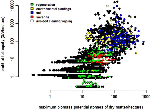
Of the 864 land-based projects on the Australian government register, 845 showed a value for both PFE and M. The market model data is plotted on Figure 1 below as coloured points; projects using the savanna burning (red), avoided deforestation (white), assisted regeneration (green), tree planting (yellow) and soil carbon enhancement (blue) methods. Description of these project methods can be found in the Supplementary Material Table A1.

Savanna burning projects are necessarily confined to the biomass values typical of tropical savannas. Avoided clearing projects occur within the range of values that are typical of where large-scale tree clearing is occurring in Australia, predominantly in the central-west of the states of Queensland and New South Wales. Environmental plantings show the widest dispersion of values, possibly because to date they have been integrated into farming activities, e.g. as shelter belts or along waterways, thereby avoiding lost agricultural production. Soil carbon projects are generally in the higher profit, higher carbon potential part of the range. Plantation projects (not plotted) are distributed within the typical range of values for commercial plantations in Australia. Supplementary Material Figure A2 gives more information on the distribution of values of PFE and M for the separate method groups in the form of box plots.

4.1. Linear model

The linear regression model in Table 2 below quantifies the observed positive relationship between PFE and M for points randomly selected across the landscape. The reported coefficient indicates an elasticity between the two variables of 1.1:1. This regression slope describes the ‘line of best fit’, indicating the more cost-efficient sources of abatement per opportunity cost. For the data points obtained from registered offsets projects, the project dummy variable predicts lower levels of PFE, indicating that the registered offset projects are more carbon cost efficient, when compared to the total set of abatement options from the Australian landscape. However, the coefficient or slope of the market model is steeper than that of the landscape model (0.25 which is added to the landscape model coefficient of 1.1) for an elasticity of roughly 1.35:1.

Table 2. linear regression model of the association between farm profits (PFE) and site biomass potential (M) for the Australian landscape and approved abatement projects.

	Estimated coefficient	Standard error	t value	Pr(>|t|)
Intercept	−1.1	0.0492	−22.36	< 2e-16 ***
loge Maximum biomass	1.1	0.0145	75.79	< 2e-16 ***
Abatement project dummy	−1.05	0.1987	−5.26	1.48e-07 ***
loge Maximum biomass * Abatement project dummy (interaction term)	0.25	0.05	4.98	6.67e-07 ***
Signif. codes: 0 ‘***’ 0.001 ‘**’ 0.01 ‘*’ 0.05 ‘.’ 0.1 ‘ ‘ 1 Residual standard error: 1.188 on 6590 degrees of freedom (4270 observations deleted due to missingness) Multiple R-squared: 0.5083, Adjusted R-squared: 0.5081 F-statistic: 2271 on 3 and 6590 DF, p-value: < 2.2e-16 Residuals: Min    1Q   Median  3Q   Max −4.3287 −0.7284  −0.0372 0.6743  5.7505

Since the market model has selected points only slightly more opportunity-cost efficient than the landscape model, this suggests that much of the dispersion around the line of best fit is either measurement error arising from the construction of the explanatory variables or that omitted variables, perhaps visible only to market participants, could explain some part of this variation.

This model explains about half the variation in the spatial association between the PFE and M variables (R-squared = 0.5083). Visual inspection of the scatterplot indicates that the relationship between M and PFE is not particularly strong within crediting method categories, but when projects of all method types are combined as in this regression, a more efficient portfolio of abatement has been selected by the offsets market.

In this figure, blue boundaries are the approved abatement projects. Red signifies the ratio of M to PFE, with the brightest red being the lowest carbon opportunity cost. White areas have no PFE data available. The highlighted abatement projects occupy regions with a high ratio of M to PFE, or in some cases with zero agricultural activity. Smaller scale projects are found in the high rainfall zones of the east and south-west coastal areas of Australia, where both maximum abatement potential and agricultural profits per hectare are much higher. Highlighted areas on Figure 2 above are described in Table 3 below.

Figure 2. Map of approved abatement projects and the biomass/agricultural profit layer (M/PFE) ratio for Australia.

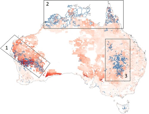
Table 3. Highlighted offset project groups, with description.

Area	Mean M and PFE values	Number of projects	Predominant project type
1. South-west Western Australia	19 t and $4	70	Human induced regeneration
2. Tropical savannas	52 t and $11	93	Savanna burning
3. Woodlands of Queensland and New South Wales	40 t and $16	357	Avoided deforestation (n = 66) and human induced regeneration/managed regrowth (n = 291)

Figure 2 and Table 3 indicate that these project types and locations, which represent a large proportion of the offset credits issued to date under the Australian scheme, correspond to those parts of the Australian continent with a highly efficient ratio of abatement potential to opportunity cost. The abatement projects registered in Australia’s voluntary offsets market occupy sites with a somewhat higher ratio of carbon potential to current land use profits, when compared to the total set of available options on the Australian agricultural land base. This should provide a higher rate of return making them more successful in the competitive market for offsets.

5. Discussion

This study’s model shows a positive relationship between variables describing carbon abatement potential, and agricultural profitability, together representing carbon opportunity cost. The implication is that NCS abatement options will be most efficient, in abatement per opportunity cost terms, when selected based on the optimization of these two variables rather than the maximization of one factor only. The model also indicates that if policy measures directed offsets projects to ‘marginal’ i.e. low profitability per unit area agricultural land, without also considering the relationship to abatement potential, this may restrict activity to less carbon efficient projects, in opposition to the objective of lowest cost abatement. This is a key consideration for the design of a policy portfolio seeking the most economically efficient emissions reduction trajectory.

Transactions costs, barriers to entry and imperfect information are all concerns when designing a market mechanism, and are under constant review by market regulators. Observed differences between the landscape and market parts of our model, and the unexplained residuals, may indicate that these factors are not accounted for in this simple model, for example:

• project and transaction costs might be lower in parts of the model’s distribution, for example savanna burning and avoided clearing, compared to the higher investment required for establishing trees on cleared land,

• landholders may accept lower rates of return because of their values and objectives, for example conservation lands,

• offset buyers may have preferences for certain project types seeking ‘quality’ and price,

• time-varying farm returns, driven by climatic and market factors, may not be captured in a single-year snapshot of Profit at Full Equity,

• properties with varying profitability per hectare may have different access to investment funds for project development.

The model could be further improved using the tools available for project assessment, for a more precise estimate of potential abatement at localized scales. Some land parcels have more than one abatement method available, requiring an ‘options’ analysis (Regan et al., 2015). Data from the bids into the Australian government’s regular auctions (Clean Energy Regulator, 2021a), such as prices tabulated by crediting method, could also be integrated as an explanatory variable. This would remove some of the informational barriers to participation identified in the market design literature, benefiting both the less well funded landholders and the buyers of credits.

Australia’s arid zone was excluded from our analysis as existing crediting methodologies cannot be applied. It covers vast areas but has low biomass, as a fire prone grassy ecosystem, and typically zero opportunity cost, being non-viable for agriculture. Further field research would be required to investigate the potential for human impact to increase carbon storage (Burrows & Chapman, 2018; Burrows et al., 2006), and would require adaptation of one of the agricultural soil carbon crediting methods, however potentially making available a new supply of credits.

NCS will compete with food supply and alternative abatement methods such as bioenergy with carbon-capture and storage (BECCS). However, the Australian Government’s zero emissions strategy relies on large quantities of annual abatement from both (Australian Government, 2021). Our modelling approach could be extended to develop a long-run supply curve for NCS.

6. Conclusions

Using two readily available spatial variables, we derived a simple but highly explanatory model of the potential for land-based emissions abatement for the Australian continent. There is a strong positive correlation between abatement potential and opportunity cost across the landscape, requiring the two factors to be optimized for lowest cost abatement. Outcomes from the competitive market for offsets as operating in Australia since 2012, incorporated into this model, show that this policy mechanism did select projects with optimum carbon abatement for a given opportunity cost.

However, this is not, as we have demonstrated, always going to be on the land with the lowest agricultural profitability per hectare. Consequently, policies directing abatement projects to ‘marginal farmland’ are not necessarily carbon-cost efficient. Such a policy may deliver other social objectives but would make the already challenging task of delivering deep emissions reductions more expensive.

Supply of land based NCS is ultimately limited by the capacity of the land sink to absorb more carbon, in soil or biomass, before reaching ‘saturation’ (Chen et al., 2019; Haverd et al., 2012; Kelley & Harrison, 2014; Ma et al., 2016), in economic terms, a long-run supply curve with diminishing returns. Estimates of maximum biomass or carbon abatement potential, and the opportunity cost of lost agricultural production, are essential inputs to developing a long-run supply curve for land-based offsets. Nations and other entities whose zero-emissions strategies rely heavily on offsets need to understand the likely cost and total quantity of such offsets. Jurisdictions with an existing land-based offset scheme could use the market outcomes as inputs to this form of analysis.

The approach used in this study could be applied to any large geographic region where similar proxy variables are available, and may assist policy makers to understand the land use policy impacts of such a large offset requirement.

Author contributions

Greg Barber: Conceptualization, Data curation, Methodology, Writing – original draft. Andrew Edwards: Writing – Review & Editing. Kerstin Zander: Conceptualization, Supervision, Writing – review and editing.

Acknowledgements

This research was conducted as part of a PhD thesis, at Charles Darwin University, with funding under the Research Training Program of the Commonwealth government.

Disclosure statement

No potential conflict of interest was reported by the author(s).

References

- Anh, N. T., Masuda, M., & Iwanaga, S. (2016). Status of forest development and opportunity cost of avoiding forest conversion in Ba Be National Park, Vietnam. Tropics. 2016.
- Anup, K., Joshi, G. R., & Aryal, S. (2014). Opportunity cost, willingness to pay and cost benefit analysis of a community forest of Nepal. International Journal of Environment, 3(2), 108–124. https://doi.org/10.3126/ije.v3i2.10522
- Ausseil, A.-G. E., Daigneault, A. J., Frame, B., & Teixeira, E. I. (2019). Towards an integrated assessment of climate and socio-economic change impacts and implications in New Zealand. Environmental Modelling & Software, 119, 1–20. https://doi.org/10.1016/j.envsoft.2019.05.009
- Australian Government. (2021). Australia's long-term emissions reduction plan. A whole-of-economy plan to achieve net zero emissions by 2050.
- Australian Government Clean Energy Regulator. (n.d.). Understanding your soil carbon project emissions reduction fund simple method guide for soil carbon projects registered under the carbon credits (carbon farming initiative - estimation of soil organic carbon sequestration using measurement and models) methodology determination 2021.
- Australian Government Department of Industry Science Energy and Resources. (2020a). National inventory report 2018: The Australian government submission to the United Nations framework convention on climate change.
- Barry, L. E., Yao, R. T., Harrison, D. R., Paragahawewa, U. H., & Pannell, D. J. (2014). Enhancing ecosystem services through afforestation: How policy can help. Land Use Policy, 39, 135–145. https://doi.org/10.1016/j.landusepol.2014.03.012
- Bednar, J., Obersteiner, M., & Wagner, F. (2019). On the financial viability of negative emissions. Nature Communications, 10(1), 1–4. https://doi.org/10.1038/s41467-019-09782-x
- Benton, T., Bailey, R., Froggatt, A., King, R., Lee, B., & Wellesley, L. (2018). Designing sustainable landuse in a 1.5 °C world: the complexities of projecting multiple ecosystem services from land. Current Opinion in Environmental Sustainability, 31, 88–95. https://doi.org/10.1016/j.cosust.2018.01.011
- Blake, A., & Eves, C. (2012). Assessment of the application of contingent valuation theory to bio-sequestered carbon. In Proceedings of the 6th International Real Estate Research Symposium.
- Blake, A. G. (2016). Carbon sequestration: Evaluating the impact on rural land and valuation approach Queensland. University of Technology.
- Bradshaw, C. J. A., Bowman, D. M. J. S., Bond, N. R., Murphy, B. P., Moore, A. D., Fordham, D. A., & Johnson, C. N. (2013). Brave new green world – Consequences of a carbon economy for the conservation of Australian biodiversity. Biological Conservation, 161, 71–90. https://doi.org/10.1016/j.biocon.2013.02.012
- Brown, C., Alexander, P., Arneth, A., Holman, I., & Rounsevell, M. (2019). Achievement of Paris climate goals unlikely due to time lags in the land system. Nature Climate Change, 9(3), 203–208. https://doi.org/10.1038/s41558-019-0400-5
- Bryan, B. A., Nolan, M., McKellar, L., Connor, J. D., Newth, D., Harwood, T., & Gao, L. (2016). Land-use and sustainability under intersecting global change and domestic policy scenarios: Trajectories for Australia to 2050. Global Environmental Change, 38, 130–152. https://doi.org/10.1016/j.gloenvcha.2016.03.002
- Bureau of Meteorology. (2021). Gridded rainfall variability metadata.
- Burrows, N., & Chapman, J. (2018). Traditional and contemporary fire patterns in the Great Victoria Desert, Western Australia (Final report, Great Victoria Desert biodiversity trust project GVD-P-17-002). D. o. B. Biodiversity and Conservation Science Division, Conservation and Attractions.
- Burrows, N. D., Burbidge, A. A., Fuller, P. J., & Behn, G. (2006). Evidence of altered fire regimes in the Western Desert region of Australia. Conservation Science Western Australia, 5(3).
- Busch, J., Engelmann, J., Cook-Patton, S. C., Griscom, B. W., Kroeger, T., Possingham, H., & Shyamsundar, P. (2019). Potential for low-cost carbon dioxide removal through tropical reforestation. Nature Climate Change, 9(6), 463–466.
- California Air Resources Board. (2021). ARB offset credit issuance table. https://ww2.arb.ca.gov/our-work/programs/compliance-offset-program.
- Carbon Credits (Carbon Farming Initiative) Act 2011 Cth.
- Carbon Market Institute. (2016). Optimising Australia's position in international carbon markets.
- Carbon Market Institute. (2017). Operationalizing Article 6 of the Paris Agreement – Perspectives of Australian business.
- Carroll, J. L., & Daigneault, A. J. (2019). Achieving ambitious climate targets: Is it economical for New Zealand to invest in agricultural GHG mitigation? Environmental Research Letters, 14(12), 124064.
- Chang, H. S., & Griffith, G. (1998). Examining long-run relationships between Australian beef prices. Australian Journal of Agricultural and Resource Economics, 42(4), 369–387. https://doi.org/10.1111/1467-8489.00058
- Chappell, A., & Baldock, J. A. (2016). Wind erosion reduces soil organic carbon sequestration falsely indicating ineffective management practices. Aeolian Research, 22, 107–116. https://doi.org/10.1016/j.aeolia.2016.07.005
- Chen, S., Arrouays, D., Angers, D. A., Martin, M. P., & Walter, C. (2019). Soil carbon stocks under different land uses and the applicability of the soil carbon saturation concept. Soil and Tillage Research, 188, 53–58. https://doi.org/10.1016/j.still.2018.11.001
- Chu, M.-Y., & Liu, W.-Y. (2021). Assessing the opportunity cost of carbon stock caused by land-use changes in Taiwan. Land, 10(11), 1240. https://doi.org/10.3390/land10111240
- Clean Energy Regulator. (2021a). 12th auction April 2021 contract portfolio.
- Clean Energy Regulator. (2021b). Area-based emissions reduction fund (ERF) projects. data.gov.au.
- Clean Energy Regulator. (2021c). Carbon abatement contract register. Clean Energy Regulator. Retrieved February 10, 2021 from.
- Clean Energy Regulator. (2021d). Emissions reduction fund project register.
- Climateworks. (2010). Low carbon growth plan for Australia. https://www.climateworksaustralia.org/wp-content/uploads/2019/10/climateworks_lcgp_australia_full_report_mar2010-compressed.pdf.
- Cohen-Shacham, E., Andrade, A., Dalton, J., Dudley, N., Jones, M., Kumar, C., Maginnis, S., Maynard, S., Nelson, C. R., & Renaud, F. G. (2019). Core principles for successfully implementing and upscaling Nature-based Solutions. Environmental Science & Policy, 98, 20–29.
- Commonwealth of Australia Department of Agriculture Water and the Environment. (2016). Australia state of the environment 2016.
- Connor, J. D., Bryan, B. A., & Nolan, M. (2016). Cap and trade policy for managing water competition from potential future carbon plantations. Environmental Science & Policy, 66, 11–22.
- Connor, J. D., Bryan, B. A., Nolan, M., Stock, F., Gao, L., Dunstall, S., & Grundy, M. (2015). Modelling Australian land use competition and ecosystem services with food price feedbacks at high spatial resolution. Environmental Modelling & Software, 69, 141–154. https://doi.org/10.1016/j.envsoft.2015.03.015
- Daigneault, A., Baker, J. S., Guo, J., Lauri, P., Favero, A., Forsell, N., Sohngen, & B. (2022). How the future of the global forest sink depends on timber demand, forest management, and carbon policies. Global Environmental Change, 76, 102582. https://doi.org/10.1016/j.gloenvcha.2022.102582
- Dean, C., Kirkpatrick, J. B., Harper, R. J., & Eldridge, D. J. (2015). Optimising carbon sequestration in arid and semiarid rangelands. Ecological Engineering, 74, 148–163. https://doi.org/10.1016/j.ecoleng.2014.09.125
- Department of Environment and Energy. (n.d.). Emissions reduction fund environmental data.
- Dong, X., Waldron, S., Brown, C., & Zhang, J. (2018). Price transmission in regional beef markets: Australia, China and Southeast Asia. Emirates Journal of Food and Agriculture, 99–106. https://doi.org/10.9755/ejfa.2018.v30.i2.1601
- Dooley, K., Stabinsky, D., Stone, K., Sharma, S., Anderson, T., Gurian-Sherman, D., & Riggs, P. (2018). Missing pathways to 1.5 °C: The role of the land sector in ambitious climate action. Climate Land Ambition and Rights Alliance.
- Eady, S., Grundy, M., Battaglia, M., & Keating, B. (2009). An analysis of greenhouse gas mitigation and carbon biosequestration opportunities from rural land use. Armidale Australia.
- Edwards, A., Archer, R., De Bruyn, P., Evans, J., Lewis, B., Vigilante, T., & Russell-Smith, J. (2021). Transforming fire management in northern Australia through successful implementation of savanna burning emissions reductions projects. Journal of Environmental Management, 290, 112568. https://doi.org/10.1016/j.jenvman.2021.112568
- Evans, M. C. (2018). Effective incentives for reforestation: Lessons from Australia's carbon farming policies. Current Opinion in Environmental Sustainability, 32, 38–45.
- Evans, M. C., Carwardine, J., Fensham, R. J., Butler, D. W., Wilson, K. A., Possingham, H. P., & Martin, T. G. (2015). Carbon farming via assisted natural regeneration as a cost-effective mechanism for restoring biodiversity in agricultural landscapes. Environmental Science & Policy, 50, 114–129.
- Fajardy, M., & Mac Dowell, N. (2017). Can BECCS deliver sustainable and resource efficient negative emissions? Energy & Environmental Science, 10(6), 1389–1426. https://doi.org/10.1039/C7EE00465F
- Fargione, J. E., Bassett, S., Boucher, T., Bridgham, S. D., Conant, R. T., Cook-Patton, S. C., Ellis, P., Falcucci, A., Fourqurean, J. W., & Gopalakrishna, T. (2018). Natural climate solutions for the United States. Science Advances, 4(11), eaat1869.
- Farmers for Climate Action. (2021). How can Australia's agriculture sector realise opportunity in a low emissions future? https://farmersforclimateaction.org.au/how-can-australias-agriculture-sector-realise-opportunity-in-a-low-emissions-future/.
- Fridahl, M., & Lehtveer, M. (2018) Bioenergy with carbon capture and storage (BECCS): Global potential, investment preferences, and deployment barriers. Energy Research & Social Science, 42, 155–165.
- Funk, J. M., Field, C. B., Kerr, S., & Daigneault, A. (2014). Modeling the impact of carbon farming on land use in a New Zealand landscape. Environmental Science & Policy, 37, 1–10. https://doi.org/10.1016/j.envsci.2013.08.008
- Fuss, S., Lamb, W. F., Callaghan, M. W., Hilaire, J., Creutzig, F., Amann, T., & Khanna, T. (2018). Negative emissions—Part 2: Costs, potentials and side effects. Environmental Research Letters, 13(6), 063002. https://doi.org/10.1088/1748-9326/aabf9f
- Gambhir, A., Butnar, I., Li, P.-H., Smith, P., & Strachan, N. (2019). A review of criticisms of integrated assessment models and proposed approaches to address these, through the lens of BECCS. Energies, 12(9), 1747.
- Golub, A., Hertel, T., Lee, H.-L., Rose, S., & Sohngen, B. (2009). The opportunity cost of land use and the global potential for greenhouse gas mitigation in agriculture and forestry. Resource and Energy Economics, 31(4), 299–319. https://doi.org/10.1016/j.reseneeco.2009.04.007
- Grafton, R. Q., Chu, H. L., Nelson, H., & Bonnis, G. (2021). A global analysis of the cost-efficiency of forest carbon sequestration.
- Griscom, B. W., Busch, J., Cook-Patton, S. C., Ellis, P. W., Funk, J., Leavitt, S. M., Lomax, G., Turner, W. R., Chapman, M., & Engelmann, J. (2020). National mitigation potential from natural climate solutions in the tropics. Philosophical Transactions of the Royal Society B, 375(1794), 20190126.
- Haverd, V., Raupach, M., Briggs, P., Canadell, J., Isaac, P., Pickett-Heaps, C., & Wang, Z. (2012). Multiple observation types reduce uncertainty in Australia's terrestrial carbon and water cycles. Biogeosciences Discussions, 9(9), 12181–12258. https://doi.org/10.5194/bgd-9-12181-2012
- Hayek, F. (1945). The use of knowledge in society. The American Economic Review, 35(4).
- Hoyos-Santillan, J., Miranda, A., Lara, A., Sepulveda-Jauregui, A., Zamorano-Elgueta, C., Gómez-González, S., Vásquez-Lavín, F., Garreaud, R. D., & Rojas, M. l. (2021). Diversifying Chile’s climate action away from industrial plantations. Environmental Science & Policy, 124, 85–89.
- Intergovernmental Panel on Climate Change. (2019). Global warming of 1.5(C An IPCC special report on the impacts of global warming of 1.5 C above pre-industrial levels and related global greenhouse gas emission pathways, in the context of strengthening the global response to the threat of climate change (sustainable development, and efforts to eradicate poverty. https://www ipcc. ch/sr15.
- Jackson, R., Canadell, J., Fuss, S., Milne, J., Nakicenovic, N., & Tavoni, M. (2017). Focus on negative emissions. https://doi.org/10.1088/1748-9326/aa94ff
- Jagtap, S., Trollman, H., Trollman, F., Garcia-Garcia, G., Parra-López, C., Duong, L., & Hdaifeh, A. (2022). The Russia-Ukraine conflict: Its implications for the global food supply chains. Foods (basel, Switzerland), 11(14), 2098. https://doi.org/10.3390/foods11142098
- Kato, E., & Yamagata, Y. (2014). BECCS capability of dedicated bioenergy crops under a future land-use scenario targeting net negative carbon emissions. Earth's Future, 2(9), 421–439. https://doi.org/10.1002/2014EF000249
- Kelley, D., & Harrison, S. (2014). Enhanced Australian carbon sink despite increased wildfire during the 21st century. Environmental Research Letters, 9(10)(10), 104015. https://doi.org/10.1088/1748-9326/9/10/104015
- Kragt, M. E., Pannell, D. J., Robertson, M. J., & Thamo, T. (2012). Assessing costs of soil carbon sequestration by crop-livestock farmers in Western Australia. Agricultural Systems, 112, 27–37. https://doi.org/10.1016/j.agsy.2012.06.005
- Lawson, K., Burns, K., Low, K., Heyhoe, E., & Ahammad, H. (2008). Analysing the economic potential of forestry for carbon sequestration under alternative carbon price paths. Australian Bureau of Agricultural and Resource Economics.
- Longmire, A., Taylor, C., & Pearson, C. J. (2015). An open-access method for targeting revegetation based on potential for emissions reduction, carbon sequestration and opportunity cost. Land Use Policy, 42, 578–585. https://doi.org/10.1016/j.landusepol.2014.09.009
- Ma, X., Huete, A., Cleverly, J., Eamus, D., Chevallier, F., Joiner, J., & Meyer, W. (2016). Drought rapidly diminishes the large net CO2 uptake in 2011 over semi-arid Australia. Scientific Reports, 6(1), 37747. https://doi.org/10.1038/srep37747
- Man, C. D., Lyons, K. C., Nelson, J. D., & Bull, G. Q. (2015). Cost to produce carbon credits by reducing the harvest level in British Columbia, Canada. Forest Policy and Economics, 52, 9–17. https://doi.org/10.1016/j.forpol.2014.12.002
- Maraseni, T. N., & Cockfield, G. (2015). The financial implications of converting farmland to state-supported environmental plantings in the Darling Downs region, Queensland. Agricultural Systems, 135, 57–65.
- Marinoni, O., Garcia, J. N., Marvanek, S., Prestwidge, D., Clifford, D., & Laredo, L. (2012). Development of a system to produce maps of agricultural profit on a continental scale: An example for Australia. Agricultural Systems, 105(1), 33–45. https://doi.org/10.1016/j.agsy.2011.09.002
- Marinoni, O., & Navarro Garcia, J. (2018). Agricultural profit map for Australia for 2010–2011. v1. CSIRO.
- McKinsey and Company. (2008). An Australian cost curve for greenhouse gas abatement. McKinsey and Company.
- Minx, J. C., Lamb, W. F., Callaghan, M. W., Bornmann, L., & Fuss, S. (2017). Fast growing research on negative emissions. Environmental Research Letters, 12(3), 035007. https://doi.org/10.1088/1748-9326/aa5ee5
- Minx, J. C., Lamb, W. F., Callaghan, M. W., Fuss, S., Hilaire, J., Creutzig, F., & Hartmann, J. (2018). Negative emissions—Part 1: Research landscape and synthesis. Environmental Research Letters, 13(6), 063001. https://doi.org/10.1088/1748-9326/aabf9b
- Monjardino, M., Revell, D., & Pannell, D. J. (2010). The potential contribution of forage shrubs to economic returns and environmental management in Australian dryland agricultural systems. Agricultural Systems, 103(4), 187–197. https://doi.org/10.1016/j.agsy.2009.12.007
- Nature4climate. (2019). Guide to including nature in nationally determined contributions. A checklist of information and accounting approaches for natural climate solutions.
- Polglase, P., Reeson, A., Hawkins, C., Paul, K., Siggins, A., Turner, J., & Opie, K. (2013). Potential for forest carbon plantings to offset greenhouse emissions in Australia: Economics and constraints to implementation. Climatic Change, 121(2), 161–175. https://doi.org/10.1007/s10584-013-0882-5
- Pour, N., Webley, P. A., & Cook, P. J. (2018). Opportunities for application of BECCS in the Australian power sector. Applied Energy, 224, 615–635.
- QGIS Development Team. (2016). QGIS geographic information system. Open Source Geospatial Foundation Project.
- R Core Team. (2013). R: A language and environment for statistical computing.
- Regan, C., Connor, J., Settre, C., Summers, D., & Cavagnaro, T. (2019). Assessing South Australian carbon offset supply and cost. Goyder institute for water research technical report series(19/03). Goyder Institute for Water Research Technical Report Series.
- Regan, C. M., Bryan, B. A., Connor, J. D., Meyer, W. S., Ostendorf, B., Zhu, Z., & Bao, C. (2015). Real options analysis for land use management: Methods, application, and implications for policy. Journal of Environmental Management, 161, 144–152. https://doi.org/10.1016/j.jenvman.2015.07.004
- Regan, C. M., Connor, J. D., Summers, D. M., Settre, C., O'Connor, P. J., & Cavagnaro, T. R. (2020). The influence of crediting and permanence periods on Australian forest-based carbon offset supply. Land Use Policy, 97, 104800. https://doi.org/10.1016/j.landusepol.2020.104800
- Richards, G. P., & Evans, D. M. (2004). Development of a carbon accounting model (FullCAM Vers. 1.0) for the Australian continent. Australian Forestry, 67(4), 277–283. https://doi.org/10.1080/00049158.2004.10674947
- Roe, S., Streck, C., Beach, R., Busch, J., Chapman, M., Daioglou, V., & Engelmann, J. (2021). Land-based measures to mitigate climate change: Potential and feasibility by country. Global Change Biology, 27(23), 6025–6058. https://doi.org/10.1111/gcb.15873
- Roxburgh, S. H., Karunaratne, S. B., Paul, K. I., Lucas, R. M., Armston, J. D., & Sun, J. (2019). A revised above-ground maximum biomass layer for the Australian continent. Forest Ecology and Management, 432, 264–275. https://doi.org/10.1016/j.foreco.2018.09.011
- Seddon, N., Smith, A., Smith, P., Key, I., Chausson, A., Girardin, C., & Turner, B. (2021). Getting the message right on nature-based solutions to climate change. Global Change Biology, 27(8), 1518–1546. https://doi.org/10.1111/gcb.15513
- Shmueli, G. (2010). To explain or to predict? Statistical Science, 25(3), 289–310. https://doi.org/10.1214/10-STS330
- Siikamäki, J., & Newbold, S. C. (2012). Potential biodiversity benefits from international programs to reduce carbon emissions from deforestation. Ambio, 41(1), 78–89. https://doi.org/10.1007/s13280-011-0243-4
- Sinnett, A., Behrendt, R., Ho, C., & Malcolm, B. (2016). The carbon credits and economic return of environmental plantings on a prime lamb property in south eastern Australia. Land Use Policy, 52, 374–381.
- The Nous Group. (2010). Outback carbon: An assessment of carbon storage, sequestration and greenhouse gas emissions in remote Australia. The Pew Environment Group-Australia and the Nature Conservancy.
- Tomich, T. P., de Foresta, H., Dennis, R., Ketterings, Q., Murdiyarso, D., Palm, C., & van Noordwijk, M. (2002). Carbon offsets for conservation and development in Indonesia? American Journal of Alternative Agriculture, 17(3), 125–137. https://doi.org/10.1079/AJAA200219
- UNFCCC. (n.d.). Clean development mechanism project register.
- Wade, C. M., Baker, J. S., Jones, J. P., Austin, K. G., Cai, Y., de Hernandez, A. B., & Creason, J. (2022). Projecting the impact of socioeconomic and policy factors on greenhouse gas emissions and carbon sequestration in U.S. Forestry and Agriculture. Journal of Forest Economics, 37(1), 127–131. https://doi.org/10.1561/112.00000545
- Weishaar, S. (2007). CO2 emission allowance allocation mechanisms, allocative efficiency and the environment: A static and dynamic perspective. European Journal of Law and Economics, 24(1), 29–70. https://doi.org/10.1007/s10657-007-9020-z
- White, R., & Davidson, B. (2016). The costs and benefits of approved methods for sequestering carbon in soil through the Australian Government’s emissions reduction fund. Environment and Natural Resources Research, 6, 99–109.
- Wood, T., Reeve, A., & Ha, J. (2021). Towards net zero: Practical policies to reduce agricultural emissions (064508798X).
- Yang, H., & Li, X. (2018). Potential variation in opportunity cost estimates for REDD+ and its causes. Forest Policy and Economics, 95, 138–146. https://doi.org/10.1016/j.forpol.2018.07.015
- Zhang, X., & Cai, X. (2011). Climate change impacts on global agricultural land availability. Environmental Research Letters, 6(1), 014014. https://doi.org/10.1088/1748-9326/6/1/014014
- Zomer, R. J., Trabucco, A., Bossio, D. A., & Verchot, L. V. (2008). Climate change mitigation: A spatial analysis of global land suitability for clean development mechanism afforestation and reforestation. Agriculture, Ecosystems & Environment, 126(1-2), 67–80. https://doi.org/10.1016/j.agee.2008.01.014