Smile and default: the role of stochastic volatility and interest rates in counterparty credit risk

Abstract

In this research, we investigate the impact of stochastic volatility and interest rates on counterparty credit risk (CCR) for FX derivatives. To achieve this we analyse two real-life cases in which the market conditions are different, namely during the 2008 credit crisis where risks are high and a period after the crisis in 2014, where volatility levels are low. The Heston model is extended by adding two Hull–White components which are calibrated to fit the EURUSD volatility surfaces. We then present future exposure profiles and credit value adjustments (CVAs) for plain vanilla cross-currency swaps (CCYS), barrier and American options and compare the different results when Heston-Hull–White-Hull–White or Black–Scholes dynamics are assumed. It is observed that the stochastic volatility has a significant impact on all the derivatives. For CCYS, some of the impact can be reduced by allowing for time-dependent variance. We further confirmed that Barrier options exposure and CVA is highly sensitive to volatility dynamics and that American options’ risk dynamics are significantly affected by the uncertainty in the interest rates.

Keywords:

• Exposure
• FX
• Heston
• Hull–White
• FDMC
• Stochastic volatility
• Stochastic interest rates
• EURUSD
• Counterparty risk

JEL Classifications:

• C63
• G01
• G12
• G17

1. Introduction

During the 2008 credit crisis, various large financial institutions experienced big losses due to counterparty credit risk (CCR) (Gregory 2010). This has made accurate assessment of future exposures of derivatives more important (Zhu and Pykhtin 2007). Given the complexity of estimating these exposures, the Black–Scholes (BS) model is often used in industry. In contrast to the valuation of single derivatives, exposure calculations are typically done on the level of counterparties and therefore require the simultaneous handling of multiple risk factors with complex interdependencies. Although the BS model gives very valuable insight into CCR, it assumes the volatility and the interest rates of the underlying risk factors to be constant. This is unrealistic and its impact in particular for long dated and path-dependent derivatives is unknown. It is more realistic to assume that the underlying driving risk factor (e.g. FX rate for cross-currency derivatives), its volatility and the interest rates are driven by stochastic processes. Here we study rigorously and for the first time, the impact of these extra degrees of freedom on exposures for various popular FX derivatives using the computationally challenging Heston-2-Hull–White (H2HW) model fully calibrated to real market data for a wide range of model and contract parameters.

In academia an important contribution to pricing FX derivatives assuming high-dimensional models is done in Grzelak et al. (2011) and Grzelak and Oosterlee (2012b), where the authors show how these high-dimensional models can be calibrated. In Schoutens et al. (2004), Detlefsen and Härdle (2007) and Chiarella et al. (2012), it is observed that stochastic volatility models that are perfectly calibrated to European options can produce different prices for path-dependent barrier options. In Ahlip and Rutkowski (2013), the importance of the interest rate dynamics for the valuation of FX options is shown. However, the choice of interest rate parameters in their work was made for illustrative purposes only. Moreover, in all these works the focus is on the possible impact on prices, whereas here we extend the analysis by looking at the impact on future exposures.

These future exposures are used to determine the valuation adjustments like CVA, DVA (Gregory 2010) and more recently KVA (Green et al. 2014). It requires simulating the future states of the risk factors and then valuing the derivative in all these future states. Recent contributions by academics and practitioners with guidelines on how to achieve this include Ng and Peterson (2009), Ng et al. (2010) and Qu and Zhu (2014). To the best of our knowledge, these techniques have not yet been used to systematically assess the impact of stochastic volatility and interest rates on exposures for real market scenarios.

In this work, the parameters of the pricing models are calibrated to European EURUSD options and EUR, USD swaptions for a range of maturities and contract specifications. In the analysis, we consider real data from periods with significantly different implied volatility surfaces and interest rate term structures. First, we consider the 2008 credit crisis, when high volatilities and moderate interest rates were common, then we turn to the aftermath of the crisis in 2014, where the volatility term structure is inverted and interest rates are low.

In these two market scenarios, we assess the model implications on CCR by analysing average and extreme-case exposures. The impact on the price of CCR is compared by looking at the widely used expected exposure (EE), expected negative exposure (ENE), expected positive exposure (EPE) and CVA. To further assess the tail effect we look at the quantiles of the future option price distribution. In order to get a complete overview, we compute these metrics for plain vanilla cross-currency-swaps (CCYS), the path-dependent up-and-out barrier Call (UOC) and American options. We find that a constant volatility model cannot capture the skew effects that are visible in the exposure profiles. The effect of skew is higher for the quantiles in comparison with the exposure profiles and increases for exotic derivatives.

The outline of this paper is as follows. In section 2, we describe the models, define the metrics and present the algorithm used to compute these metrics. The data and the calibration procedure is presented in Section 3. In section 4, we systematically analyse the impact for the different derivatives under different market conditions. Section 5 summarizes our findings.

2. Problem formulation

2.1. Models

The main model used in this paper is the H2HW model, where Heston is extended with two HW processes to incorporate the stochastic dynamics of the interest rates. To assess the impacts, this model serves as a benchmark. Assuming these dynamics one can price cross-currency and fixed-income products. As in the Heston case, the SDE for the variance process enables us to capture the volatility smile. The four-dimensional dynamics of the H2HW model are given by:(1a) (1b) (1c) (1d) (1e) where the variance process (1b(1b) ) is a CIR process with as the mean-reverting speed, as the level of the long-term mean, the so-called volatility-of-volatility. The short rate (1c(1c) ) (or (1d(1d) )) are both modelled by a HW process with () as the mean-reverting speed, () as the yield level deduced from the forward curve and () the short-rate volatility of the domestic (foreign) interest rate process. Note that the drift adjustment for comes from the change of measure to the domestic risk-neutral measure (Grzelak and Oosterlee 2012a, b).

This model allows to price hybrid products whose pay-off depends on different stochastic components of the model. Pricing a European option means finding such that(2)

Via Feynman-Kac, one can show that the time-reversed pricing mechanism u of a contingent claim has to satisfy the following PDE(3) (4) where .

In order to assess the impact of stochastic volatility we compare against the Black–Scholes-2-Hull–White (BS2HW) model which assumes a deterministic volatility. In this case, we consider the following two possibilities:

(i)	Using the ATM implied volatility at maturity of the derivative;
(ii)	Using a piecewise constant volatility function which is aligned with the ATM implied volatility curve over all maturities.

In appendix 1, we show the effective volatilities for the different models.

On the other hand, the impact of stochastic interest rates is assessed by looking into the Heston model with constant interest rates and .

2.2. Derivatives

We consider CCYS, Up-and-out Barrier Call (UOC) and American Put/Call options. The former is the simplest derivative connecting FX and fixed-income markets and is highly relevant from the perspective of exposure and outstanding trading volumes. In addition, UOC and American options are interesting because of their path-dependence and early-exercise possibilities. More technical details about the pricing of these derivatives can be found in Simaitis (2014) and Filipović (2009).

2.2.1. Cross-currency swap

A cross-currency swap is a derivative where the buyer pays interest and a notional in one currency and receives in another. Through this work we assume a swap where the buyer receives interest in USD and pays it in EUR. We present results for fixed notional cross-currency basis swaps where both legs are floating and notionals are exchanged at inception and maturity. At-the-money (ATM) refers to the case where all cash flows (notional exchanges and future payments) are based on a domestic and foreign principal amount that is implied by the FX () spot rate. For the in-the-money (ITM) and out-of-the-money (OTM) cases, the FX rates 1.25 and 0.75 are used.

CCYS differ from the other derivatives considered here in the sense that it is possible to compute its prices analytically without assuming an SDE to drive the FX rate. For exposure however, future scenarios are needed and for that the FX rate needs to be driven by a model.

2.2.2. Up-and-out call option

Next, we look into an UOC option. This first-order exotic option terminates (value becomes 0) when the underlying FX rate exceeds a predefined barrier level B, but otherwise delivers a pay-off equal to that of a European call. The price of an UOC option with barrier B, strike K and maturity T equals:(5)

where . Note that future exposure as well as prices are now path-dependent because of the knockout probability.

2.2.3. American options

The holder of an American option is able to receive the pay-off upon request any time before maturity. In practice, these options are approximated as Bermudan options with many time points at which such early exercise is allowed. Clearly, by increasing the number of time points the option will converge to the American option.

For pricing, time is discretized by taking number of uniformly distributed time points between 0 and T with . At each exercise time, the exercise value (given by the pay-off function) and the continuation value of the option are compared in a backward induction scheme. The pay-off function and the continuation value for the option at discrete time are, defined as:(6) (7)

where is the option value at time .

It is assumed that the holder of the option exercises the option when the pay-off is higher than or equal to the continuation value, after which the contract terminates. At maturity , the option value is equal to the pay-off value.

The following recursive scheme is set-up to price a Bermudan option:(8)

In comparison to Barrier options the exercise of an American option is even more dependent on the chosen model. For barrier options, the exercise level is equal to the barrier which is static, for Americans options however, this exercise level is determined by the continuation value which depends on the chosen model and the future state variables. For example, in the simple BS world with no dividends/foreign exchange rate and positive domestic risk-free rate it is not beneficial to exercise an American Call option. However, this is not the case when both rates are time-dependent. As we describe later in more detail, American options seem to be very sensitive to the uncertainty in fixed-income markets.

2.3. Risk metrics

For CCR, not only the price is important, but also the possible value dynamics after the deal has been settled. In this work, we use several measures to quantify CCR.

First define the positive exposure at a future time as:(9)

where u(t) is the (mark-to-market) value of a financial derivative contract at time t. Negative exposure is defined as the minimum instead of the maximum of u(t) and zero. The EPE and ENE at a future time are given by:(10a) where is the filtration at time . The expectation is calculated under risk-neutral measure . Similarly, the expected discounted positive exposure (EPE*) and expected discounted negative exposure (ENE*) at a future time are given by:(11a) where, D(0, t) is the discount factor. EPE* (ENE*) gives the expected loss of the buyer (seller) of the contract in case he is in the money and the counterparty defaults, in present terms. This makes them of prime importance when computing credit value adjustment (CVA), which is defined as:(12)

where R is the so-called recovery rate and PD(0, t) the risk-neutral probability of the counterparty default between 0 and t (Zhu and Pykhtin 2007). Here, for simplicity we use: , where is the survival probability of a counterparty up to time t and this can be computed with the help of a hazard rate:(13)

Following Whetten and Adelson (2004), this hazard rate can expressed as a function of the annual CDS premiums and the recovery rate. For a full derivation of this expression we refer to Simaitis (2014). Note that for the computation of Debt Value Adjustment (DVA), in equation (12(12) ), the EPE* should be replaced by ENE*.

EE is the probability-weighted average future value of the derivative at time t:(14)

This metric shows the dynamics of the mean contract value. Note that in case the derivative has a positive pay-off EE is equal to EPE. This is the case for the UOC and American options that we look into. Moreover, if there is no early exercise opportunity, the options discounted EE is just the price of the option as shown in Simaitis (2014). The discounted EE is useful in future collateral requirement calculations and is given by:(15)

The exposures (EE/EPE/ENE) provide insight into the mean properties of the contract value distribution which are mostly used to attach price tags to risk. However, from the point of risk, one is also interested in the worst-case scenarios which in our work are analysed by looking at the quantiles of the future contract value distribution. The quantile functions () represent the best (worst) case scenario the buyer can face at a future time t and is defined as:(16)

Note that these quantiles differ from the potential future exposure (PFE), which need to be modelled under the real-world measure. In that case the future scenarios need to be generated by historically calibrated models (Stein 2014). The effect of different model specifications is expected to be similar under real-world or risk-neutral measure. That is why in this paper, the scenario generation is done under the risk-neutral measure both for the computation of exposures and the quantiles.

2.4. Algorithm

For the computation of various valuation adjustment, one can create a new valuation framework as is done in, for example, Burgard and Kjaer (2011) and Brigo et al. (2014), but here we choose another approach. We compute the exposures from the distribution of the future value of a derivative. The valuation of the CCYS is performed by combining Monte Carlo (MC) simulations with analytical pricing. As there is no general analytic price for American or Barrier options under the H2HW dynamics, we apply the Finite Difference Monte Carlo (FDMC) method as described in de Graaf et al. (2014). The pseudo-code for the algorithm is as follows:

(i)	Select the number of time points ;
(ii)	Construct a joint mesh grid for every modelled underlying risk factor;
(iii)	On this grid, solve the PDE backwards in time using the FD method, and store these price grids for every time point;
(iv)	Select the number of paths and set ;
(v)	Use the MC method to simulate realizations of the underlying risk factors at , where ;
(vi)	For each of the simulated states, compute the respective derivative price by interpolation on the price grid;
(vii)	When early exercise/termination is allowed, set the derivative price to the exercise/termination value for paths which have been exercised/terminated at time t;
(viii)	Calculate the exposure metrics using the resulting distribution of the derivative prices;
(ix)	If needed discount the exposure metrics;
(x)	If take and go to step 2.4, else quit.

By definition the exposure of an early exercise option equals zero once the option is exercised; otherwise, the exposure is equal to the value of the option.

For the scenario generation, we use the Euler discretization for the FX and interest rates. As the Euler scheme is proved to be inefficient for the simulation of the volatility dimension, the QE scheme as described in Andersen (2008) is used. For the scenario generation we used paths and 100 time points such that in all test cases, the relative standard error of the mean was smaller than 1%.

To solve the pricing PDE (2.1) on a grid in every dimension, we developed an FD implementation following Haentjens and in ’t Hout (2012). Note that pricing claims on underlyings driven by the H2HW model requires solving a four-dimensional PDE which, in the case of exotic options, will result in large computational requirements.¹ The number of grid points used for the pricing grids equals 80, 40, 20 and 20 in s-, v-, - and -dimension, respectively, and 100 points in time. Using this number of points we have compared European call option prices obtained by the finite difference method with a Monte Carlo simulation with paths and 100 time points. For both periods we found that the relative difference was smaller than . Furthermore, the error analysis in Simaitis (2014) shows that this number of points is sufficient to accurately (relative error smaller than ) price UOC and American options.² Because of the large computational demands, the discretized equation is solved via the alternating direction implicit (ADI) method which is numerically stable and computationally attractive as it only inverts sparse matrices. Because of its second-order convergence we choose the Hundsdorfer-Verwer scheme (see e.g. Craig and Sneyd 1988, Hundsdorfer and Verwer 2003, in ’t Hout and Welfert 2009).

3. Market data and model calibration

As noted earlier, the assessment of the additional degrees of freedom and their impact is performed by simulating exposures for derivatives on the EURUSD FX rate.³ We start by calibrating the models to the prices observed in the market during two different periods. The calibrated parameters are then used in computing the implied densities and exposure metrics. In the following section, the differences between the models are analysed by comparing these metrics.

3.1. Data

Our data-set contains market data from two intrinsically different periods. We analyse the impact of the different models in these two distinct market scenarios in order to get a robust view of the model implications. The first data-set presented in figure 1(a) contains implied EURUSD volatilities as observed in 2008 on the 29th of September which represents the market conditions during the 2008 credit crisis. The second data-set is extracted from the market as seen on 2 December 2014 and is presented in figure 1(b). Comparison the two data-sets reveal that:

(i)	In 2008, during the crisis, the volatility was relatively high for short maturities, but steadily decreasing with time-to-maturity for higher maturities;
(ii)	The reverse is true in the case of 2 December 2014—volatilities are at historically low levels, but are increasing for larger maturities;
(iii)	In both cases, the volatility smile ‘flattens’ as maturity increases;
(iv)	Qualitatively speaking, the skew is more profound in 2014. In addition, the skew is also more visible in the implied smiles of the shorter maturity vanilla options.

Figure 1. EURUSD implied volatilities as a function of moneyness, which is defined as , for different expiries and different periods.

Figure 2. Domestic (USD) and foreign (EUR) yield curves.

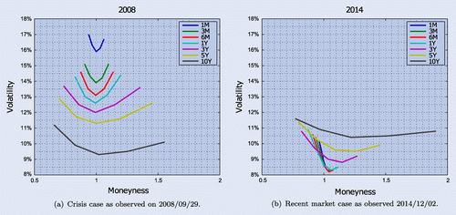
Table 1. Absolute calibration errors measured as .

Moneyness	10% call		25% call		ATM		25% put		10% put
T	2008 (%)	2014 (%)	2008 (%)	2014 (%)	2008 (%)	2014 (%)	2008 (%)	2014 (%)	2008 (%)	2014 (%)
6M	0.35	1.20	0.50	0.70	0.78	0.11	0.33	0.11	0.68	0.14
1Y	0.26	1.00	0.57	0.53	0.79	0.03	0.32	0.18	0.72	0.19
3Y	0.46	0.01	0.14	0.07	0.12	0.17	0.28	0.26	0.67	0.31
10Y	0.42	0.26	0.23	0.04	0.15	0.05	0.13	0.13	0.45	0.04

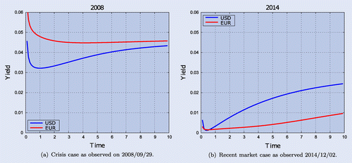
The Hull–White components used in the H2HW model allow to fit the term structure of the market interest rates. The fitted yield curves of the periods are presented in figure 2. The comparison reveals the following:

(i)	Interest rate levels are moderate in 2008 and quite low in 2014;
(ii)	The rate differences are large for shorter tenors, but decrease with time in 2008 and vice versa in 2014;
(iii)	In 2008, domestic (USD) rate is lower than foreign (EUR) an the other way around in 2014.

3.2. Calibration

The calibration procedure used in this paper is described in more detail in Simaitis (2014). For each strike, K and maturity T implied volatilities, combined with yield curve data are converted into call option prices . The goal of the calibration procedure is then to find parameter vector such that the following is minimized:(17)

Note that for the H2HW model, 14 parameters have to be calibrated which is a demanding task for the commodity hardware. Therefore, the parameter estimation is performed in stages:

(i)	The Hull–White parameters are calibrated to fit the prevailing yield curve and swaption data using analytic expressions. We used co-terminal swaptions that terminate in 10 years (1x9, 2x8, 3x7, 4x6, 5x5, 6x4, 7x3, 8x2 and 9x1), as these swaptions can also be used to replicate the CVA of a swap that matures in 10 years, as is shown in  Sorensen and Bollier (1994).
(ii)	The Heston model is fitted to the FX implied volatility surface using the COS method as presented in Fang and Oosterlee (2008) using constraint optimization. In the fitting procedure market, volatilities are converted to prices which are then used to calibrate the parameters.
(iii)	The correlations between the observable factors (exchange and interest rates) are estimated using historical time-series data4;
(iv)	H2HW parameters are filled in with values from the previous stages. The remaining correlations then are fitted using grid search algorithm5 over the feasible values.6

The resulting implied volatility errors are shown in table 1. The discrepancies are highest close to the strike where the convexity tends to be high. This is especially visible for the cases with short maturities where the smile is most profound. An increase in error level can be observed as maturities increase which could be explained by the non-uniformity of options in time. The data contains more options of shorter maturities hence the goal function penalizes errors in shorter maturities more than those in the long term. The mean relative errors expressed as percentages of the market implied volatility averaged at 4.4% in 2008 and 3.0% in 2014 and are mostly dominated by far out-of-money strikes. We have also done this calibration routine by minimizing implied volatilities instead of prices and the results were similar. An improvement of this calibration could be achieved by weighting the errors by the corresponding option liquidity if such data were available.

Table 2. CVA for a CCYS for the different models and moneyness levels. The CDS spreads range from 100 to 400 bps. The recovery rate is assumed to be constant at 0% and the CVA is quoted as a percentage of the notional.

		2008			2014
	bps	H2HW (%)	BS2HWATM vol (%)	BS2HW piecewise vol (%)	H2HW (%)	BS2HWATM vol (%)	BS2HW piecewise vol (%)
ITM	100	1.88	1.81	1.87	1.58	1.69	1.60
	200	3.58	3.46	3.57	3.02	3.22	3.06
	300	5.13	4.96	5.12	4.34	4.62	4.37
	400	6.54	6.32	6.53	5.53	5.89	5.60
ATM	100	0.87	0.71	0.85	0.57	0.69	0.56
	200	1.64	1.35	1.62	1.08	1.31	1.05
	300	2.34	1.92	2.31	1.53	1.86	1.50
	400	2.96	2.42	2.92	1.93	2.35	1.89
OTM	100	0.26	0.12	0.20	0.15	0.15	0.09
	200	0.49	0.23	0.37	0.28	0.28	0.18
	300	0.69	0.32	0.52	0.39	0.39	0.25
	400	0.86	0.39	0.65	0.49	0.49	0.30

 

Table 3. Mean Differences () between the exposures of a 10-year floating vs floating CCYS modeled by the Heston 2 Hull–White model or the BS model with constant or piecewise constant volatility. The differences are in bps relative to the notional for three different moneyness levels and two different periods.

		ITM		ATM		OTM
		2008	2014	2008	2014	2008	2014
EE	Constant volatility	2.1	6.6	2.3	7.5	3.4	10.4
	Piecewise constant volatility	2.0	2.9	2.8	3.1	4.7	3.8
EPE	Constant volatility	66.4	138.5	167.2	151.2	159.0	8.1
	Piecewise constant volatility	14.6	37.8	16.6	3.2	64.9	56.3
ENE	Constant volatility	68.4	145.1	169.5	158.6	162.3	18.5
	Piecewise constant volatility	16.6	40.6	18.1	5.9	60.4	52.6

 

Table 4. Mean Differences () between the quantiles of a 10-year floating vs floating CCYS modeled by the Heston 2 Hull–White model or the BS model with constant or piecewise constant volatility. The differences are in bps relative to the notional for three different moneyness levels and two different periods.

		ITM		ATM		OTM
		2008	2014	2008	2014	2008	2014
	Constant volatility	1010	206	1258	251	1672	332
	Piecewise constant volatility	531	510	659	628	873	832
	Constant volatility	818	1351	1034	1683	1391	2240
	Piecewise constant volatility	167	434	205	532	261	703

The calibrated parameters can be found in appendix 2.

4. Case studies

The assessment of the stochastic interest rate is made by comparing the results of H2HW to Heston and the stochastic volatility by contrasting H2HW to BS2HW. For the CCYS, we first look at the CVA as a percentage of the notional P, which is computed as a discrete sum over time (with the number of equidistant time points):(18)

where M can be the full H2HW, Heston or BS2HW model with constant or piecewise constant volatility and is computed with the help of survival probabilities as explained in section 2.3.

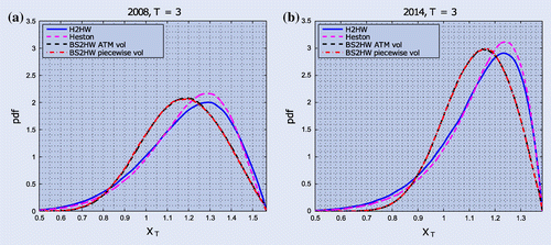
Figure 3. Densities of the FX rate generated by calibrating H2HW, Heston and BS2HW with constant and piecewise constant volatility to 2008 (left) or 2014 (right) data. Figure 3(a) and (b) shows the unconditional distribution after years, whereas figure 3(c) and (d) shows the distributions after years.

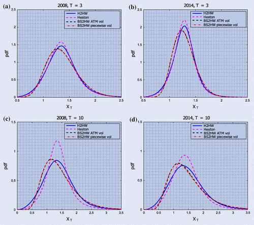
Figure 4. Exposures metrics under H2HW and BS2HW for a 10-year floating vs floating CCYS for three different moneyness levels and two different periods. ATM refers to the case where all cash flows (notional exchanges and future payments) are based on a domestic and foreign principal amount that is implied by the FX () spot rate. For the ITM and OTM cases, the FX rates 1.25 and 0.75 are used.

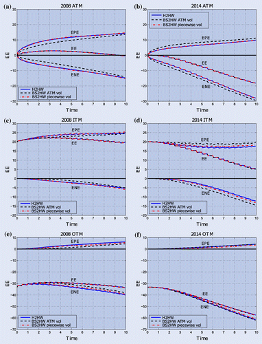
Figure 5. 2.5 and 97.5% quantiles under H2HW and BS2HW for a 10-year floating vs floating CCYS for three different moneyness levels and two different periods. ATM refers to the case where all cash flows (notional exchanges and future payments) are based on a domestic and foreign principal amount that is implied by the FX () spot rate. For the ITM and OTM cases, the FX rates 1.25 and 0.75 are used.

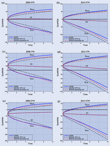
Figure 6. Densities of the FX rate after three years generated by calibrating H2HW, Heston and BS2HW with constant and piecewise constant volatility to 2008 (left) or 2014 (right) data. The densities are conditioned on , where the barrier is set at 110% of .

To further quantify the differences between the models we look at the mean difference (MD) of exposures over time relative to the notional P expressed in basis points (19(19) ). This way we can assess model differences as the swap spread difference which is independent of the counterparties creditworthiness. As a reference we take the exposure computed by the full H2HW model and compare the exposures modelled under Heston or BS2HW with constant and piecewise constant volatility:(19)

where is the exposure metric (EE, EPE, ENE or quantile) modelled under H2HW and the exposure metric modelled under M where again M can be the Heston or BS2HW model with constant or piecewise constant volatility. For the barrier and American options we look at the relative differences of CVA where we take the H2HW value as a reference:(20)

Figure 7. EE and 97.5% quantiles computed under H2HW and BS2HW for a 3 year UOC option with barrier level at for the two periods.

Figure 8. EE computed under H2HW and BS2HW for 3 year American call and put options two periods.

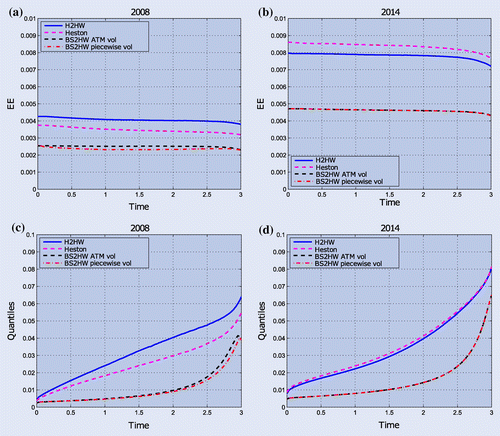
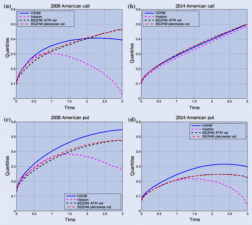
Figure 9. 97.5% quantiles computed under H2HW and BS2HW for 3 year American call and put options for the two periods.

4.1. Cross-currency swaps

The first derivative to be analysed is the domestic receiver CCYS. Since exposure of swaps heavily depends on interest rate risk, we disregard the Heston model with constant interest rates.

4.1.1. Densities

In figure 3, we show the densities for the future FX rates for two maturities and the two time periods. We see that the Heston model implies fatter left tails. Another observation is that adding stochastic volatility results in a shifted peak. Furthermore, the uncertainty in the interest rates makes the peak milder and produces more likely tail events, in particular for longer maturities.

4.1.2. Exposures and CVA

Figure 4 presents the three exposure metrics for the two periods and for different moneyness levels.

A first observation is that the difference between the one-sided exposures (EPE and ENE) modelled by H2HW or BS2HW with piecewise constant volatility is small for an ATM traded swap. The differences are larger for other moneyness levels. When we compare 2008 with 2014, we see that the exposures modelled in 2008 are more positive than in 2014. This is in line with the future yields as presented in figure 2.

Table 5. Differences from and relative to H2HW CVA for UOC options for the 2008 and 2014 periods. The recovery rate is fixed at 0% and the counterparty’s credit spread is assumed to be 50 or 200 bps.

		2008 (%)	2014 (%)
50 bps	Heston	13.6	7.9
	BS2HW ATM vol	38.6	40.4
	BS2HW piecewise vol	42.5	40.5
200 bps	Heston	13.6	7.8
	BS2HW ATM vol	38.7	40.4
	BS2HW piecewise vol	42.5	40.5

The CVA of the CCYS is presented in table 2, for different CDS spreads, ranging from 0 to 400 bps. We can see that both in 2008 and in 2014, the Black Scholes model with ATM volatility is significantly different than the H2HW model. The Black Scholes model with piecewise volatility is closer to the H2HW model, but in the ITM and OTM case, the difference is more profound which can be explained by the larger skew effect.

The mean differences for exposures (EE, EPE and ENE) are shown in table 3. For EE the differences for both BS models are in the range of 10 bps upfront. However for the one-sided exposures (EPE and ENE), the differences are in the range of 50 bps for the piecewise constant volatility model and even in the range of 150 bps for the constant volatility model. These results suggest that the skew impact is significant, but is generally lower when the term structure of volatility is fully taken into account.

4.1.3. Quantiles

Figure 5(a) and (b) presents the evolution of the quantiles for the 10-year ATM CCYS under H2HW and BS2HW with constant and piecewise constant volatility. Clearly, the differences in quantiles are more pronounced than the differences in exposures. The quantiles modelled by a piecewise constant volatility BS model are close to the H2HW quantiles at the start, but diverge towards maturity. This is similar for the ITM and OTM cases as shown in figure 6(c)–(f).

In table 4 we show the MDs of the quantiles in basis points. The differences are in the range of 500 bps for the piecewise constant volatility model and even in the range of 1500 bps for the constant volatility model. These observations lead to the conclusion that the effects of volatility smile on quantiles cannot be captured neither by a deterministic nor by a piecewise constant volatility version of the BS model.

Table 6. Differences between models expressed as CVA differences from and relative to the H2HW model for American call and put options for the 2008 and 2014 periods. The recovery rate is fixed at 0% and the counterparty’s credit spread is assumed to be 50 or 200 bps.

		Call		Put
		2008 (%)	2014 (%)	2008 (%)	2014 (%)
50 bps	Heston	27.6	5.2	21.4	24.1
	BS2HW ATM vol	5.0	2.8	0.6	7.9
	BS2HW piecewise vol	7.7	2.9	3.3	8.0
200 bps	Heston	27.3	5.2	21.1	23.8
	BS2HW ATM vol	5.0	2.8	0.6	7.9
	BS2HW piecewise vol	7.7	2.9	3.3	7.9

4.2. Barrier options

In this section, we look into path-dependent UOC barrier options on the EURUSD exchange rate. In addition to the comparisons between H2HW and BS2HW with the different volatilities, we also compute the exposures with the Heston model, such that we can investigate the impact of stochastic interest rates. For the barrier options, we took a maturity of three years. For these type of maturities, barrier levels up to 130% are common choices. We have investigated the barrier levels from 110 to 130% and found that the results were similar. Here, we show results for three year UOC options with barrier level 110%.

4.2.1. Densities

The densities shown in figure 6(a) and (b) are computed by conditioning on the FX rate being lower than barrier level B during the lifetime of the option. We observe the effect of stochastic volatility by noting the fatter left tails of the distributions generated by the Heston models. In addition, the BS densities peak further away from the up-and-out barrier level B. Again the stochasticity of the interest rates results in a lower peak for the H2HW model compared to Heston.

4.2.2. Exposures and CVA

The probability of hitting the barrier impacts the dynamics of the EE as shown in figure 7(a) and (b). The initial barrier prices () for the different models are considerably different. These differences between the models persist over time. Comparing 2008 to 2014, we can see that the EEs in 2008 are lower than in 2014 due to lower volatility levels. Next to that the difference between the stochastic volatility and the deterministic volatility models is bigger in 2014 than in 2008 because of the relatively higher skew in 2014.

In table 5, we can see that the mean relative differences in CVA is always more than 7% and can be up to 42%. Note that the Heston model is closer to the H2HW model compared to the BS2HW models. Therefore we can conclude that for barrier options the smile has a bigger impact on CVA than the stochastic interest rates.

4.2.3. Quantiles

Again the differences in quantiles computed by the different models are bigger than those in EEs as figure 7(c) and (d) show. We found that the mean relative differences in 97.5% quantiles between a deterministic volatility model and the full H2HW model can be more than 70% in 2008.

One important observation about the quantile is that the model risk for up-and-out barrier options is smaller if the quantile increases. In other words: the difference between the models becomes smaller for higher quantiles. This is due to the fact that the pay-off function of a barrier option has a maximum value, namely , therefore the maximum exposure is also limited by this value. Whereas, in the case of European options the difference can even increase for higher quantiles.

4.3. American options

Most traded options are American style and thus allow for early exercise. The early exercise decision depends on the continuation and the intrinsic value of the claim at future time points. The implied exercise boundary can be highly model dependent and therefore it is interesting to explore its effect on exposure dynamics. In this section we consider American put and call options for the two different time periods and analyse the effect of stochastic volatility and rates on the exposure metrics.

4.3.1. Exposures and CVA

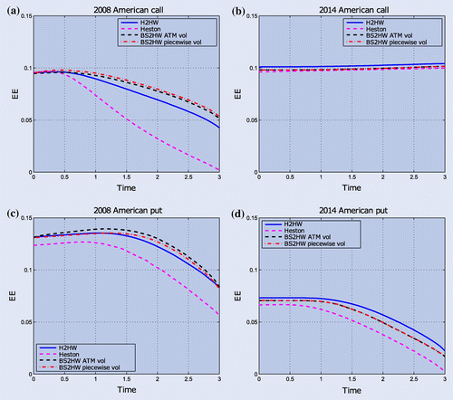
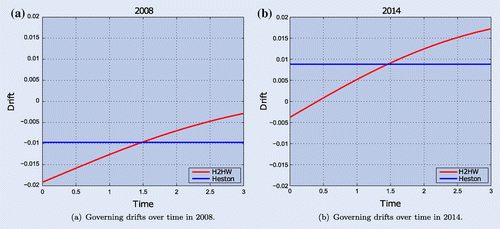
The EE profiles for American calls, shown in figure 8(a) and (b), reveal that in 2008 the EE is dropping, whereas in 2014 it does not drop and even slightly increases. This can be explained by looking at the yields shown in figure 2. In FX options the foreign yield plays a similar role as dividends in equity options. It is well known that for zero dividend paying stocks the value of American call options are equal to their European counterparts. When dividends are non-zero, it can be profitable to exercise call options early. We will see a similar effect induced by the interplay between the foreign and domestic interest rate which will be controlled by the stochasticity of the rates. In 2008, the foreign Euro yield is higher than the domestic USD yield which causes a negative drift and implies early exercise with a drop in the exposure as a result. In 2014, the domestic USD yield is higher than the foreign Euro yield such that the drift is positive and because of this positive drift, there is no early exercise such that the EE does not drop. In appendix 3, the governing drifts over time for the different periods are shown.

For the exposures of put options, shown in figure 8(c) and (d), we see that it is always profitable to exercise early as the profiles are decreasing. Looking at the different models we see that the EE modelled under the Heston dynamics is significantly different. Independent of the option type, the Heston model is always underestimating the EE. We can quantify this by looking into the relative differences of the CVAs. Again, as a reference we take the H2HW model and compare the CVAs modelled under Heston and BS2HW with constant and piecewise constant volatility. The resulting differences are shown in table 6.

4.3.2. Quantiles

Figure 9 shows that the effect seen in exposures is again larger for quantiles. Also for quantiles, the 2014 American call mimics a European quantile profile because of the lack of exercise opportunity. In all other cases, we see that the quantile computed with the Heston model is decreasing close to maturity relatively more than the other models. We have computed the mean relative difference between quantiles computed by H2HW and Heston and found that the difference can be more than 30%. For the quantiles and for EE we see that the BS2HW models are closer to H2HW than Heston such that we can conclude that for American options, the stochastic interest rates have a bigger impact than stochastic volatility.

5. Discussion

In this research, we assess the impact of uncertainty in the interest rates and volatility on CCR metrics of EURUSD derivatives and CCYS. The analysis is performed by looking at two distinct periods with different market conditions. These periods include the 2008 credit crisis, where high volatilities and moderate interest rates were present, and the aftermath of the crisis in 2014, where volatility is low and fixed income market yields are close to zero. We investigate the impact of using a H2HW, Heston or Black–Scholes-2-Hull–White with constant or piecewise constant volatility model on exposure metrics of plain vanilla CCYS, UOC and American put and call options.

In the case of CCYS, we see that the BS model with piecewise constant volatility approximates the H2HW model better than a constant volatility model. However, the accuracy of this approximation depends on moneyness of the trade. We found that the EE of an ITM or OTM trade modelled by a piecewise constant volatility model is significantly different from the EE modelled by a full H2HW model. Furthermore, the assessment of extreme scenarios (in our study represented by a 2.5% or 97.5% quantile) is much more sensitive to the stochasticity of the volatility levels. This also depends on the market conditions, as we observed that the difference between the models with and without skew is bigger in 2014 than in 2008.

When analysing the UOC options we confirm their sensitivity to volatility skew. We see that the models that are calibrated to the same European option market can lead to more than 40% differences in the UOC CVAs. This confirms and extends the results that are described in earlier work. We see that for barrier options the stochastic volatility has a bigger impact on exposure and quantiles than do stochastic interest rates.

Similarly to the previous cases, American options are significantly affected by the risk in volatility levels. Moreover, we observed a substantial difference in models with and without uncertainty in yield curves. The Heston model with constant interest rates shows a different early exercise strategy than the models with stochastic interest rates. We reason this to be due to the possible sign change of the drift of the FX process when short rates are modelled as SDEs. Because of this different early exercise strategy, the stochasticity of interest rates had the biggest impact on the exposure of American options.

In conclusion, we confirmed that the inclusion/exclusion of stochastic volatility has a significant impact on exposure dynamics. Especially, those of more complex path-dependent derivatives. The impact of stochastic interest rate varies from small to large depending on the situation in the fixed-income markets. Moreover, this impact is most significant in the case of American options. All results are magnified when one looks at the quantiles of the future option price distribution. These factors have to be taken into account, and a piecewise constant volatility model is not enough, when considering expected or worst-case scenario outcomes in CCR.

Disclosure statement

No potential conflict of interest was reported by the authors.

Acknowledgements

The authors would like to thank Dr Peter Spreij, Dr Patrik Karlson and Dr Shashi Jain for their useful comments. In addition, the financial support by the Dutch Technology Foundation [STW project 12214] is gratefully acknowledged.

Notes

The opinions expressed in this work are solely those of the authors anddo not represent in any way those of their current and past employers.

1 In case of European options the PDE can be reduced to a two-dimensional PDE by switching to the forward measure.

2 In this analysis, the convergence in the number of time and grid points is studied and shown to be of order higher than 1. Next to that, limiting cases of the H2HW option prices are compared to Black Scholes prices and the relative error for both options is shown to be smaller than .

3 Note that in the EURUSD case USD is the domestic currency and EUR is the foreign.

4 These correlations are assumed to be equal in 2008 and 2014.

5 In our experiments, option values were rather insensitive to the changes in these correlations, so the grid was much coarser than in previous stages.

6 Note that the correlations have to be picked such that the covariance matrix remains positive semi-definite.

8 Contribution statement The initial code was written by Simaitis under the guidance of de Graaf and further revised and finalized by de Graaf. The numerical tests and analysis have been conducted jointly by Simaitis and de Graaf in close collaboration with Hari and Kandhai. The data and explanations of the market conventions is provided by Hari and Kandhai. The paper is written by Simaitis and de Graaf and further revised by all authors.

Appendix 1

Implied volatility bootstrapping

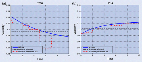
The resulting different volatility levels that are used for the BS2HW models are shown in figure A1 together with the mean of the volatility over time when it is modelled as an SDE in the H2HW model.

Appendix 2

Calibrated parameters

The parameters obtained by the described calibration procedure for the two periods are shown in table B1. A closer examination of the parameters reveals that the volatility term structure is reflected in the initial and long-term stochastic volatility levels. Also, the larger skew in 2014 is reflected in the more negative . Other than this, the calibrated parameters seem to be somewhat similar between the two periods.

Table B1. Calibrated parameters for the H2HW model for the 2008 and 2014 periods.

	Parameter	2008	2014
FX rate		1.41	1.25
Volatility		0.0204	0.0071
		0.2174	0.2475
		0.0039	0.0160
		0.1000	0.1037
Domestic IR		0.0297	-0.0036
		0.0100	0.0100
		0.0105	0.0087
Foreign IR		0.0489	0.0002
		0.0100	0.0100
		0.0067	0.0070
Correlations		-0.0796	-0.2079
		0.1572	0.1572
		-0.2957	-0.2957
		-0.9000	-0.8500
		-0.7500	-0.6000
		0.6432	0.6432

Appendix 3

Drift over time

The governing drifts () over time for the different models are presented in figure C1.

1

Figure C1. Effective volatilities over time for the three different models and two different periods.

0

Figure C2. Net drifts of the FX SDE in 2008 and 2014. Note that for the Heston model this drift is constant, whereas for H2HW and BS2HW this is not the case.

References

- Ahlip, R. and Rutkowski, M., Pricing of foreign exchange options under the Heston stochastic volatility model and CIR interest rates. Quant. Finance, 2013, 13(6), 955–966. Available online at: http://www.tandfonline.com/doi/abs/10.1080/14697688.2013.769688.
- Andersen, L., Simple and efficient simulation of the Heston stochastic volatility model. J. Comput. Finance, 2008, 11(3), 1–42.
- Brigo, D., Capponi, A. and Pallavicini, A., Arbitrage-free bilateral counterparty risk valuation under collateralization and application to credit default swaps. Math. Finance, 2014, 24(1), 125–146. Available online at: http://onlinelibrary.wiley.com/doi/10.1111/j.1467-9965.2012.00520.x/full.
- Burgard, C. and Kjaer, M., Partial differential equation representations of derivatives with bilateral counterparty risk and funding costs. J. Credit Risk, 2011, 7(3), 75–94. Available online at: http://library.agri-bank.com/pdfTemp/A7645.pdf.
- Chiarella, C., Kang, B. and Meyer, G.H., The evaluation of barrier option prices under stochastic volatility. Comput. Math. Appl., 2012, 64(6), 2034–2048. Available online at: http://www.sciencedirect.com/science/article/pii/S0898122112003215.
- Craig, I.J.D. and Sneyd, A.D., An alternating-direction implicit scheme for parabolic equations with mixed derivatives. Comput. Math. Appl., 1988, 16(4), 341–350.
- de Graaf, C.S.L., Feng, Q., Kandhai, B.D. and Oosterlee, C.W., Efficient computation of exposure profiles for counterparty credit risk. Int. J. Theor. Appl. Finance, 2014, 17(4), 1–24.
- Detlefsen, K. and Härdle, W.K., Calibration risk for exotic options. J. Derivatives, 2007, 14(4): 47–63.
- Fang, F. and Oosterlee, C.W., A novel pricing method for European options based on Fourier-cosine series expansions. SIAM J. Sci. Comput., 2008, 31(2), 826–848. Available online at: http://epubs.siam.org/doi/abs/10.1137/080718061.
- Filipović, D., Term-structure models a graduate course, 2009. Available online at: http://books.google.com/books?hl=en&lr=&id=KqcSh6CavaAC&oi=fnd&pg=PA2&dq=Term-Structure+Models+A+graduate+course&ots=-YXNKBMlZ_&sig=-DKhdsYHYLhiODI0Ivq9ut4eFkY.
- Green, A., Kenyon, C. and Dennis, C., KVA: Capital valuation adjustment by replication. Risk, 2014, 27(12).
- Gregory, J., Counterparty Credit Risk, 2010 (Wiley Online Library: Chichester).
- Grzelak, L.A. and Oosterlee, C.W., On cross-currency models with stochastic volatility and correlated interest rates. Appl. Math. Finance, 2012a, 19(1), 1–35.
- Grzelak, L.A. and Oosterlee, C.W., On cross-currency models with stochastic volatility and correlated interest rates. Appl. Math. Finance, 2012b, 19(1), 1–35.
- Grzelak, L.A., Oosterlee, C.W. and Van Weeren, S., The affine Heston model with correlated Gaussian interest rates for pricing hybrid derivatives. Quant. Finance, 2011, 11(11), 1647–1663.
- Haentjens, T. and in ’t Hout, K.J., ADI finite difference schemes for the Heston--Hull--White PDE. J. Comput. Finance, 2012, 16(1): 83–110.
- Hundsdorfer, W. and Verwer, J.G., Numerical Solution of Time-dependent Advection–Diffusion–Reaction Equations, 2003 (Springer: Berlin).
- in ’t Hout, K.J. and Welfert, B.D., Unconditional stability of second-order ADI schemes applied to multi-dimensional diffusion equations with mixed derivative terms. Appl. Numer. Math., 2009, 59(3--4): 677–692. Available online at: http://linkinghub.elsevier.com/retrieve/pii/S016892740800055X.
- Ng, L. and Peterson, D., Potential future exposure calculations using the BGM model. Wilmott J., 2009, 1(4), 213–225. Available online at: http://doi.wiley.com/10.1002/wilj.20.
- Ng, L., Peterson, D. and Rodriguez, A.E., Potential future exposure calculations of multi-asset exotic products using the stochastic mesh method. J. Comput. Finance, 2010, 14(2), 119–153.
- Qu, D. and Zhu, D., Grid Monte Carlo in portfolio CVA valuation. Wilmott Mag., 2014, 70, 64–70.
- Schoutens, W., Simons, E. and Tistaert, J., A perfect calibration! Now what? Wilmott Mag., 2004, 66–78.
- Simaitis, S., Stochastic interest rate and volatility implications for the exposure of FX options. MSc Thesis, University of Amsterdam, 2014.
- Sorensen, E.H. and Bollier, T.F., Pricing swap default risk. Financ. Anal. J., 1994, 50(3), 23–33. Available online at: http://www.jstor.org/stable/10.2307/4479743.
- Stein, H.J., Fixing underexposed snapshots measures---Proper computation of credit exposures under the real world and risk neutral measures. Technical report, Bloomberg LP, 2014. Available online at: http://ssrn.com/abstract=2365540.
- Whetten, M. and Adelson, M. Credit Default Swap (CDS) Primer, Fixed Income Research, Nomura Securities International, Inc., 12 May, 2004.
- Zhu, S. and Pykhtin, M., A guide to modeling counterparty credit risk. GARP Risk Rev., 2007, 37, 16–22. Available online at: http://papers.ssrn.com/sol3/papers.cfm?abstractid=1032522.