A structural Heath–Jarrow–Morton framework for consistent intraday spot and futures electricity prices

Abstract

The framework is based on stochastic processes with economic interpretations and is consistent with the initial forward price curve

© 2019 iStockphoto LP
1. Introduction

In recent years, the electricity intraday markets have gained increased popularity: the traded volume at the German/Austrian intraday market has grown by 30.3 percent from May 2016 to May 2018 (EPEX 2017, 2018). In the same time period, European day-ahead trading increased by 10.4 percent. Furthermore, comparing the year 2017 with 2018, European power derivatives gained 19 percent in traded volume (EEX 2019). Since different electricity contracts exhibit different price behaviour such as spikes in the day-ahead spot but not in futures prices, it is a rising challenge in energy finance to define a single model that allows for a joint simulation of power prices at intraday spot and futures markets.

In this paper, we suggest a Heath–Jarrow–Morton framework for modelling electricity prices. The framework is consistent with the current forward term structure (i.e. the price forward curve) and we motivate each mathematical component by an economic interpretation. Furthermore, we discuss the computation of intraday spot and futures prices within this framework and we show how options on futures contracts can be priced. A new approach is the use of structural models for day-ahead spot price modelling within the Heath–Jarrow–Morton framework.

The starting point for the Heath–Jarrow–Morton (HJM1) approach for electricity prices is the fictitious forward price or forward kernel.2 The forward kernel $f_t\left(\tau \right)$, $t\le \tau$, is the price at time t of a forward contract delivering electricity instantly at time τ. It follows that the price at t of a futures contract delivering from ${\tau }_1$ to ${\tau }_2$ is the averaged forward kernel during the delivery period, i.e. (1) $F_t({\tau }_1,{\tau }_2)=\frac{1}{{\tau }_2-{\tau }_1}{\int }_{{\tau }_1}^{{\tau }_2}{f}_t\left(u\right)\mathrm{d}u,t\le {\tau }_1.$(1) In the HJM framework for interest rates the forward rate is modelled instead of the short rate (cf. Brigo and Mercurio 2006). Therefore, modelling the forward kernel instead of the day-ahead spot price3 makes this an HJM approach for power prices. Furthermore, just like in the HJM framework for interest rates, the forward kernel itself is not a traded product at the market but through equation (1) its derivatives are.

Several models for the forward kernel $f_t\left(\tau \right)$ have been introduced by Clewlow and Strickland (1999), Hinz et al. (2005), Koekebakker and Ollmar (2005), Benth and Koekebakker (2008), Kiesel et al. (2009). They define the forward kernel dynamics driven by Brownian motions. However, since the day-ahead spot prices show spikes, these models have drawbacks. Therefore, there is a need for a forward kernel model that allows for spikes in relatively short delivery periods (day-ahead spot contracts) but smooths these out for longer delivery periods (futures contracts). The theoretical HJM framework of Benth et al. (2019) introduces forward kernel dynamics driven by Brownian motions and pure jump Lévy processes. Their framework is similar to ours but touches on the differences between the real-world and the pricing measure. A difference to our approach is that we have motivated the modelling ingredients by economic arguments and allow for an easy transfer of day-ahead structural models to an HJM setting, which we also show in Section 3.

In the literature, the use of more than one probability measure has been challenged: Lyle and Elliott (2009), Caldana et al. (2017) assume a single probability measure, for example. This is supported by the fact that it is not clear which equivalent measure should be the pricing measure Q. Since electricity is a non-storable commodity and buy-and-hold strategy arguments are not valid, it is not clear what the relation between the price of electricity contracts and the money market account is (Bessembinder and Lemmon 2002). This also implies that the market is incomplete and that there are (possibly) infinitely many equivalent pricing measures. Again, this leaves the choice of pricing measure unclear.

We follow the idea of Caldana et al. (2017) that the prices of day-ahead spot and futures contracts both should be computed by equation (1(1) $F_t({\tau }_1,{\tau }_2)=\frac{1}{{\tau }_2-{\tau }_1}{\int }_{{\tau }_1}^{{\tau }_2}{f}_t\left(u\right)\mathrm{d}u,t\le {\tau }_1.$(1) ). This actually sounds right intuitively since, for example in the German markets, day-ahead spot contracts are traded at least 12 hours before delivery. In other countries such as the USA the terminology is different: the day-ahead spot price is commonly referred to as the forward price (Longstaff and Wang 2004). Even in Europe, with the increasing popularity of the intraday markets, we observe a shift in terminology. Weron (2014) remarks that the term spot is used more and more frequently for the real-time or intraday market. We will always explicitly state to which spot market we refer.

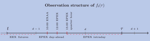
In this paper, we even propose to extend equation (1(1) $F_t({\tau }_1,{\tau }_2)=\frac{1}{{\tau }_2-{\tau }_1}{\int }_{{\tau }_1}^{{\tau }_2}{f}_t\left(u\right)\mathrm{d}u,t\le {\tau }_1.$(1) ) to the intraday market. Figure 1 gives an example of the development of the forward kernel $f_t\left(\tau \right)$ and how it becomes observable at the German/Austrian market. First the forward kernel $f_t\left(\tau \right)$ is only (partly) observable through EEX futures contracts. Then the Austrian EXAA and two German EPEX day-ahead spot auctions are held, after which the EPEX intraday spot market opens.

Figure 1. Observation structure of $f_t\left(\tau \right)$ for the German electricity market and a fixed delivery time τ. The red marked lines and time points are the (indirect) observation moments. The lines with d−1 and d stand for the start of day d−1 and d.

Furthermore, we show how the classical models described by Schwartz and Smith (2000), Lucia and Schwartz (2002) fit into our framework. We also show how other more general day-ahead spot price models can be used to fit into our model. A particular new example we introduce in this paper is to use structural models in the context of an HJM framework. We also apply our framework to the setting of multi-factor models.

This paper is structured as follows: section 2 introduces a model for the forward kernel based on the economic intuition that there are two driving components behind the forward kernel. The first component is the equilibrium of supply and demand at delivery time and the second is a general noise from partially informed traders or illiquidity at trading time t. Successively, in section 2.2 and section 2.3 the futures and option prices are computed, respectively. Section 3 contains the above explicitly mentioned examples for the market equilibrium process, while section 4 concludes.

2. HJM framework

In section 2.1, we will define a model for the forward kernel motivated by economic interpretations. Using this model in sections 2.2 and 2.3, we derive the prices of futures contracts and options on futures contracts, respectively. Section 2.4 gives an overview of the prices for different electricity contracts for the example of the German market.

2.1. Forward kernel

The forward kernel $f_t\left(\tau \right)$ is the price at time t of a forward contract delivering 1 MW instantly at time τ. Throughout the rest of this paper, we interpret t as the trading time and τ as the delivery time.

For $\tau \ge 0$ let $X^{\tau }=\{X_t^{\tau };t\ge 0\}$ and $Y=\{Y_t;t\ge 0\}$ be two independent, a.s. càdlàg stochastic processes on the complete probability space $(\mathrm{\Omega },\mathcal{F},P)$ taking values in $\mathbb{R}$ and ${\mathbb{R}}^n$, respectively. Furthermore, assume that the processes $X^{\tau }$ for each $\tau \ge 0$ and Y are adapted to the filtration $\{{\mathcal{F}}_t;t\ge 0\}$, which satisfies the usual conditions, i.e. $\{{\mathcal{F}}_t;t\ge 0\}$ is right-continuous and ${\mathcal{F}}_0$ contains all P-null sets. The filtration generated by Y and $X^{\tau }$ augmented by all P-null sets automatically fulfils these conditions. Finally, let $g:{\mathbb{R}}^n\to \mathbb{R}$ be a function such that $g\left(Y_t\right)$ is real-valued stochastic process.

We have two strong economic interpretations for these two stochastic processes: we interpret the n-dimensional process $Y_t$ as the randomness or the state of the market, where each component of $Y_t$ stands for a (random) facet of the market, e.g. demand, load, or weather predictions. The function g maps the state of the market state $Y_t$ to its corresponding price. Combining the fact that our inspiration came from the class of structural models for day-ahead spot price modelling and the fact that it gives the basic structure to the forward kernel, we call the pair $(g,Y_t)$ the structural component. Often we will also only call $Y_t$ the structural component.

The process $X_t^{\tau }$ is called the market noise because it accounts for the incomplete market information of all market participants and illiquidity of the market. An example of incomplete market information is the uncertainty of weather predictions: nobody knows with complete certainty about the future weather or temperature. With these interpretations, we define the forward kernel:

Definition 2.1

(Forward kernel)

We define the forward kernel at trading time t and delivery time τ as $f_t\left(\tau \right):=X_t^{\tau }\mathbb{E}\left[g\left(Y_{\tau }\right)|{\mathcal{F}}_t\right],$ where $X_t^{\tau }$ is the market noise at trading time t for the delivery time τ and $(g,Y_{\tau })$ the structural component at delivery time τ.

We use the notation $X_t^{\tau }$ to emphasize that the market noise is a stochastic process in the trading time t but can depend on the delivery time τ, whereas the structural component $Y_{\tau }$ only depends on delivery time. Economically, this makes sense since the imbalance of supply and demand at delivery time τ determines the price independent of the trading time t at which we predict this imbalance. However, the market noise is the disturbance of this prediction originating from market participants with incomplete market information, which intuitively depends on both the trading time t and the delivery time τ they are trying to predict.4 Although we call $X_t^{\tau }$ the market noise, it can also be interpreted as a measure transformation (or Radon–Nikodym derivative, see Remark 2.7) or as a general additional component that introduces an additional degree of freedom in the modelling process.

Assumption 2.2

(Market noise)

The process $X^{\tau }=\{X_t^{\tau };t\ge 0\}$ with its interpretation as market noise for delivery time τ is defined as multiplicative stochastic noise. We assume that it is an a.s. positive càdlàg martingale with expectation one, i.e. $\mathbb{E}{X}_t^{\tau }=1$ for all $\tau \ge t\ge 0$. In particular, we assume that the initial value $X_0^{\tau }=1$ a.s. for all $\tau \ge 0$.

Assumption 2.3

(Structural component)

We assume that $Y=\{Y_t;t\ge 0\}$ is a ${\mathbb{R}}^n$-valued càdlàg stochastic process. In particular, we assume that the initial value equals $Y_0=y_0\in {\mathbb{R}}^n$ a.s. such that $g\left(y_0\right)=f_0\left(0\right)$, where $f_0\left(\tau \right)$ is the initial price forward curve (PFC) for delivery time τ, which we assume to be known (cf. Remark 2.4). Furthermore, as a technical assumption we need that $\mathbb{E}|g\left(Y_t\right)|<\mathrm{\infty }$ for all $t\ge 0$. Finally, although we assume that $g\left(Y_t\right)$ can take all values in $\mathbb{R}$, including negative values, we assume that its expectation $\mathbb{E}g\left(Y_t\right)>0$ is strictly positive. The economic interpretation behind this assumption is that we do not expect negative forward prices to occur.

With these assumptions, the sign of the forward kernel is uniquely determined by the structural component Y and the process $X^{\tau }$ cannot influence it. Furthermore, the expectation $\mathbb{E}{f}_t\left(\tau \right)$ is fully determined by the structural component $Y_{\tau }$ and independent of trading time t (cf. Lemma 2.6).

Remark 2.4

(Initial price forward curve $f_0\left(\tau \right)$)

In this framework, the initial price forward curve (PFC), denoted by $f_0\left(\tau \right)$, plays an important role: it determines the expectation of the forward kernel $f_t\left(\tau \right)$. There are many studies that describe how one can construct a PFC from market prices such as Caldana et al. (2017), Kiesel et al. (2018), for example. In practice, every energy utility has an in-house PFC. In the following, we will therefore assume that the PFC is known.

As discussed by Benth and Paraschiv (2018), another interesting possibility is to use a Musiela parametrisation for the forward kernel. This parametrisation is given by the bijective mapping $(t,\tau )\mapsto (t,u):=(t,\tau -t)$ of ${\mathbb{R}}^2$ on itself. In their work, Benth and Paraschiv (2018) propose a spatio-temporal random field model in the context of an HJM framework under the Musiela parametrisation, where they call the time to maturity u the spatial component. They disentangled the temporal from spatial effects on the dynamics of forward prices and found that the temporal noise was non-Gaussian. In our context, we could directly use the Musiela parametrisation by substituting $\tau =u+t$.

Theorem 2.5

For fixed $\tau \ge 0$, the forward kernel process $f\left(\tau \right):=\left\{f_t\right(\tau );t\ge 0\}$ is an adapted stochastic process. Furthermore, $f\left(\tau \right)$ is a.s. càdlàg.

Proof.

By definition, $f\left(\tau \right)$ is a stochastic process. Moreover, since we assumed $X_t^{\tau }$ to be ${\mathcal{F}}_t$-measurable and since the conditional expectation $Z_t^{\tau }:=\mathbb{E}\left[g\right(Y_{\tau }\left)|{\mathcal{F}}_t\right]$ is always ${\mathcal{F}}_t$-measurable, the ${\mathcal{F}}_t$-measurability of $f_t\left(\tau \right)$ follows immediately. Because the filtration satisfies the usual conditions, $Z_t^{\tau }$ has a càdlàg modification (Karatzas and Shreve 1998, Chapter 1, Theorem 3.13). Since the conditional expectation $Z_t^{\tau }$ is uniquely defined up to null sets, we can choose this modification and the result follows by the assumption that $X_t^{\tau }$ is càdlàg.

Since we assume that $X^{\tau }$ and Y both a.s. start at a deterministic value, we assume without loss of generality that ${\mathcal{F}}_0$ is generated by Ω and all P-null sets. This in particular implies that $\mathbb{E}g\left(Y_{\tau }\right)=\mathbb{E}\left[g\right(Y_{\tau }\left)|{\mathcal{F}}_0\right]$, a fact we will exploit in the next lemma.

Lemma 2.6

For fixed $\tau \ge 0$ the forward kernel process $f\left(\tau \right):=\left\{f_t\right(\tau );t\ge 0\}$ is a martingale. Furthermore, its expectation is given by $\mathbb{E}{f}_t\left(\tau \right)=\mathbb{E}g\left(Y_{\tau }\right)=f_0\left(\tau \right)$ for all $0\le t\le \tau$.

Proof.

The product of two independent martingales clearly is a martingale. Furthermore, it follows immediately from Assumption 2.2 and 2.3 that $\begin{array}{rl}\mathbb{E}{f}_t\left(\tau \right)& =\mathbb{E}\left[X_t^{\tau }\right]\mathbb{E}\left[\mathbb{E}\left[g\left(Y_{\tau }\right)|{\mathcal{F}}_t\right]\right]=\mathbb{E}g\left(Y_{\tau }\right)\\ & =X_0^{\tau }\mathbb{E}\left[g\left(Y_{\tau }\right)|{\mathcal{F}}_0\right]=f_0\left(\tau \right)\end{array}$ by the independence of $X_t^{\tau }$ and $Y_t$.

Lemma 2.6 also imposes a condition for the expectation $\mathbb{E}g\left(Y_{\tau }\right)$ of the structural component, which can be used to calibrate the structural component Y and function g after the PFC $f_0\left(\tau \right)$ has been determined. If one wants to obtain a model that is consistent with an existing PFC $f_0\left(\tau \right)$, one needs to choose and calibrate g and Y such that $\mathbb{E}g\left(Y_{\tau }\right)=f_0\left(\tau \right)$.

Remark 2.7

(Risk-neutral measure)

In the previous discussion, we considered the measure space $(\mathrm{\Omega },\mathcal{F},P)$ equipped with the measure P. However, as seen in Lemma 2.6 and will be seen in Lemma 2.12, the forward kernel and its induced futures prices are martingales under the measure P. This is an argument in favour of viewing P as the risk-neutral measure or pricing measure in this framework, making this framework especially suitable for pricing derivatives. However, if one wants to simulate market prices through this framework, one needs to derive the dynamics of the market prices under the real-world measure which can be done by a suitable measure change, as is discussed by Benth et al. (2019). Under the real-world measure the expectation is then no longer constant in trading time t, which is a phenomenon that is supported by plenty of empirical evidence. In particular in the case of the continuous intraday market this is studied by the findings of Kiesel and Paraschiv (2017).

Another view on this framework is achieved by defining the following measure: the τ-forward measure $P^{\tau }$ defined by its Radon–Nikodym derivative (2) $\frac{\mathrm{d}{P}^{\tau }}{\mathrm{d}P}{|}_{{\mathcal{F}}_t}=\frac{1}{X_t^{\tau }}$(2) could be used for this purpose. Using the τ-forward measure and Bayes' theorem for conditional expectations, we can rewrite Definition 2.1 $f_t\left(\tau \right)=X_t^{\tau }{\mathbb{E}}_P\left[g\right(Y_{\tau }\left)|{\mathcal{F}}_t\right]={\mathbb{E}}_{P^{\tau }}\left[X_{\tau }^{\tau }g\right(Y_{\tau }\left)|{\mathcal{F}}_t\right].$ The latter term can be defined as $S_t:=X_t^{t}g\left(Y_t\right),$ which yields a general spot price model. This is another argument in favour of viewing P and $P^{\tau }$ as equivalent pricing measures (where $P^{\tau }$ is viewed as a forward pricing measure). As discussed in the introduction electricity markets are incomplete and therefore it is possible that multiple equivalent pricing measures exist. In this setting, the choice of the stochastic process $X_t^{\tau }$ can be viewed as the choice of delivery time specific pricing measure $P^{\tau }$ in light of equation (2(2) $\frac{\mathrm{d}{P}^{\tau }}{\mathrm{d}P}{|}_{{\mathcal{F}}_t}=\frac{1}{X_t^{\tau }}$(2) ). If the noise $X_t:=X_t^{\tau }$ is chosen to be independent of the delivery time τ, so is the τ-forward measure $P^{\tau }$.

2.2. Futures contracts

As discussed in section 1, the forward kernel can be used to compute the price of futures contracts. In the following, we assume the interest rate to equal r = 0 for notational convenience. Of course, when one assumes $r\ne 0$, discounting has to be taken into account. In Remark 2.13, we have some notes on how to change our framework to include discounting. Furthermore, we assume that all prices are normalized, meaning that we assume all prices to be in Euro/MWh as usual.

Definition 2.8

(Futures contract price)

For $0\le t\le {\tau }_1<{\tau }_2$, we call $F_t({\tau }_1,{\tau }_2):=\frac{1}{{\tau }_2-{\tau }_1}{\int }_{{\tau }_1}^{{\tau }_2}{f}_t\left(u\right)\mathrm{d}u$ the price of a futures contract at time t delivering 1 MW continuously from ${\tau }_1$ to ${\tau }_2$.

Since we denote all prices in Euro/MWh, the price that one pays at time t when one buys a futures contract delivering 1 MW from ${\tau }_1$ to ${\tau }_2$ is given by $({\tau }_2-{\tau }_1)F_t({\tau }_1,{\tau }_2)$, where we assume that ${\tau }_2-{\tau }_1$ is measured in hours.

Example 2.9

(Day-ahead spot price)

We compute the day-ahead spot price as a futures contract. It is auctioned at day d−1 at hour a and delivered at day d from h:00 until $(h+1)$:00 o'clock, i.e. $S(d,h):=F_{t_{d-1}^a}\left(t_d^h,t_d^{h+1}\right).$ Here $t_d^h$ denotes the time at day d and hour h.

The next theorem shows that the framework is consistent with cascading.5 It also shows that there are no arbitrage opportunities in the sense that the cost of a futures contract delivering for 1 year is the same as the cost of its four quarters, for example.

Proposition 2.10

(Consistency of cascading)

Let $0\le {\tau }_0<{\tau }_1<{\tau }_2<\cdots <{\tau }_n$ be delivery times, then we have $({\tau }_n-{\tau }_0)F_t({\tau }_0,{\tau }_n)=\sum _{i=1}^n({\tau }_i-{\tau }_{i-1})F_t({\tau }_{i-1},{\tau }_i)$ for all $t\ge 0$.

Proof.

This follows directly from Definition 2.8 and the countable additivity of the Lebesgue integral.

Lemma 2.11

Fix $0\le t<\tau$. If $u\mapsto f_t\left(u\right)$ is almost surely continuous on $(\tau -ϵ,\tau ]$ for some $ϵ>0,$ then we have $\underset{s\to {\tau }^{-}}{lim}{F}_t(s,\tau )=f_t\left(\tau \right)$ almost surely.

Proof.

We compute $\begin{array}{rl}& \underset{s\to {\tau }^{-}}{lim}{F}_t(s,\tau )\\ & =\frac{\underset{s\to {\tau }^{-}}{lim}{\int }_s^{\tau }{f}_t\left(u\right)\mathrm{d}u}{\underset{s\to {\tau }^{-}}{lim}\tau -s}=\frac{\underset{s\to {\tau }^{-}}{lim}-f_t\left(s\right)}{-1}=f_t\left(\tau \right)\end{array}$ where we used L'Hôpital's rule for the second equality.

The previous lemma shows that the price of a futures contract delivering for just an instant equals the forward kernel. This supports the naming of the quantity $f_t\left(\tau \right)$ as forward kernel.

Lemma 2.12

Assume that the price forward curve $\tau \mapsto f_0\left(\tau \right)$ is continuous. Then the futures price process $F({\tau }_1,{\tau }_2):=\left\{F_t\right({\tau }_1,{\tau }_2);t\ge 0\}$ is a martingale. Its expectation is given by $\mathbb{E}{F}_t({\tau }_1,{\tau }_2)=F_0({\tau }_1,{\tau }_2)=\frac{1}{{\tau }_2-{\tau }_1}{\int }_{{\tau }_1}^{{\tau }_2}{f}_0\left(u\right)\mathrm{d}u$ for all $0\le t\le {\tau }_1<{\tau }_2$.

Proof.

Since the price forward curve is continuous, it is bounded on any compact set, in particular intervals of the form $[{\tau }_1,{\tau }_2]$, and therefore integrable on compacts. Direct computation with Fubini's Theorem shows that for $0\le t<s$ $\begin{array}{rl}\mathbb{E}\left[F_s\right({\tau }_1,{\tau }_2\left)|{\mathcal{F}}_t\right]& =\mathbb{E}\left[\frac{1}{{\tau }_2-{\tau }_1}{\int }_{{\tau }_1}^{{\tau }_2}{f}_s\left(u\right)\mathrm{d}u|{\mathcal{F}}_t\right]\\ & =\frac{1}{{\tau }_2-{\tau }_1}{\int }_{{\tau }_1}^{{\tau }_2}\mathbb{E}\left[f_s\right(u\left)|{\mathcal{F}}_t\right]\mathrm{d}u,\end{array}$ where the latter exists and therefore all integrals exist. Combination with Lemma 2.6 now proves the theorem.

Remark 2.13

($r\ne 0$)

If we assume that $r\ne 0$, the futures price depends on the settlement date. There are two possibilities: settlement takes place either through continuous payments6 during the delivery period or at once at the end of the delivery period. If $d_t\left(\tau \right)$ denotes the discount factor of a future payment at time τ to an earlier time t, the price of a futures contract is given by $F_t({\tau }_1,{\tau }_2)=\frac{1}{{\int }_{{\tau }_1}^{{\tau }_2}{d}_t\left(u\right)\mathrm{d}u}{\int }_{{\tau }_1}^{{\tau }_2}{d}_t\left(u\right)f_t\left(u\right)\mathrm{d}u$ for continuous settlement and by $F_t({\tau }_1,{\tau }_2)=\frac{1}{({\tau }_2-{\tau }_1)d_t\left({\tau }_2\right)}{\int }_{{\tau }_1}^{{\tau }_2}{d}_t\left(u\right)f_t\left(u\right)\mathrm{d}u$ for settlement at the end of delivery.

2.3. Options on futures contracts

In this section, we assume that the market noise is given by a geometric Brownian motion (GBM) without drift, i.e. $\mathrm{d}{X}_t^{\tau }=X_t^{\tau }\mathrm{\Sigma }(t,\tau {)}^T\mathrm{d}{W}_t$ where $\mathrm{\Sigma }(t,\tau )$ is a deterministic m-dimensional volatility vector and $W_t$ is an m-dimensional Brownian motion. The strong solution of $X_t^{\tau }$ is given by $X_t^{\tau }=\exp \left({\int }_0^t\mathrm{\Sigma }(u,\tau {)}^T\mathrm{d}{W}_u-\frac{1}{2}{\int }_0^t\mathrm{\Sigma }(u,\tau {)}^T\mathrm{\Sigma }(u,\tau )\mathrm{d}u\right).$ In this case, $X_t^{\tau }$ satisfies Assumption 2.2 if $\mathrm{\Sigma }(u,\tau )$ is square integrable in u. But this is already a requirement for the stochastic integral to be defined.

Example 2.14

(Hull–White market noise dynamics)

A possible choice for Σ is a two-factor forward dynamic similar to Kiesel et al. (2009), which is also discussed in a geometric setting by Fanelli and Schmeck (2018) for pricing options on futures. This volatility structure is extended by Latini et al. (2018) in an additive setting. They discussed a two-factor volatility structure comparable to the two-factor Hull–White model for interest rate modelling (Brigo and Mercurio 2006, Section 4.2.5). It is given by $\mathrm{\Sigma }(t,\tau {)}^T:=({\mathrm{e}}^{-\kappa (\tau -t)}{\sigma }_1,{\sigma }_2\left(\tau \right)),$ where ${\sigma }_1>0$ is the additional short-term volatility, $\kappa >0$ is the rate of decay of the short-term volatility, and ${\sigma }_2\left(\tau \right)>0$ is the long-term volatility at delivery time τ. A convenient choice for ${\sigma }_2$ is a piecewise constant function, being constant on delivery periods of tradable futures contracts. An advantage of this choice is that we can use the calibration methods for $X_t^{\tau }$ as discussed by Kiesel et al. (2009), Latini et al. (2018), Fanelli and Schmeck (2018).

Throughout the rest of this section, we assume that the conditional expectation of the structural component decomposes into an affine structure:

Definition 2.15

(Affine structural component decomposition)

We say the structural component $(g,Y_t)$ allows for the affine structural component decomposition, if there exist deterministic functions $(t,\tau )\mapsto A_t^{\tau }\in {\mathbb{R}}^{n\times n}$ and $(t,\tau )\mapsto B_t^{\tau }\in {\mathbb{R}}^n$ such that the following decomposition holds: (3) $\mathbb{E}\left[g\right(Y_{\tau }\left)|{\mathcal{F}}_t\right]=g(A_t^{\tau }{Y}_t+B_t^{\tau })$(3) a.s. for all $\tau \ge t\ge 0$.

This decomposition can be motivated by the fact that our best guess at time t for the state of market $Y_{\tau }$ at time τ is an affine transformation of the current state of the market $Y_t$. This is also the main idea behind Kalman filtering, for example. If the decomposition holds, this merely states that this best guess should hold under the transformation g, which transforms the market state into a price.

It follows immediately that the forward kernel is given by (4) $f_t\left(\tau \right)=X_t^{\tau }g(A_t^{\tau }{Y}_t+B_t^{\tau }),$(4) when the affine structural component decomposition assumption is satisfied. Furthermore, the futures price of Definition 2.8 can be rewritten as $F_t({\tau }_1,{\tau }_2)=\frac{1}{{\tau }_2-{\tau }_1}{\int }_{{\tau }_1}^{{\tau }_2}{X}_t^{u}g(A_t^u{Y}_t+B_t^u)\mathrm{d}u$ for all $0\le t\le {\tau }_1<{\tau }_2$. As immediate consequences we obtain:

Lemma 2.16

If $(g,Y_t)$ allows for the affine structural component decomposition, then $\mathbb{E}\left[g\right(Y_{\tau }\left)|{\mathcal{F}}_t\right]=\mathbb{E}\left[g\right(Y_{\tau }\left)|Y_t\right]$.

Lemma 2.17

Under assumption of the decomposition of Definition 2.15, the forward kernel conditioned on $Y_t$ is lognormally distributed, i.e. $\begin{array}{rl}& \left(f_t\right(\tau )|Y_t=y)\\ & \sim LN\left(\ln \left[g\right(A_t^{\tau }y+B_t^{\tau }\left)\right],{\int }_0^t\mathrm{\Sigma }(u,\tau {)}^T\mathrm{\Sigma }(u,\tau )\mathrm{d}u\right).\end{array}$

Proof.

Using equation (4(4) $f_t\left(\tau \right)=X_t^{\tau }g(A_t^{\tau }{Y}_t+B_t^{\tau }),$(4) ), we compute $P\left(f_t\left(\tau \right)\le x|Y_t=y\right)=P\left(X_t^{\tau }g(A_t^{\tau }y+B_t^{\tau })\le x\right),$ which shows the result since $X_t^{\tau }\sim LN(0,{\int }_0^t\mathrm{\Sigma }(u,\tau {)}^{\mathrm{T}}\mathrm{\Sigma }(u,\tau )\mathrm{d}u)$.

Theorem 2.18

If $(g,Y_t)$ allows for the affine structural component decomposition, then the first two moments of the futures price $F_t({\tau }_1,{\tau }_2)$ exist and are given by $\mathbb{E}\left[F_t\right({\tau }_1,{\tau }_2)|Y_t=y]=\frac{1}{{\tau }_2-{\tau }_1}{\int }_{{\tau }_1}^{{\tau }_2}g(A_t^{u}y+B_t^u)\mathrm{d}u$ and $\begin{array}{rl}& \mathbb{E}\left[F_t\right({\tau }_1,{\tau }_2{)}^2|Y_t=y]\\ & =\frac{1}{({\tau }_2-{\tau }_1{)}^2}{\int }_{{\tau }_1}^{{\tau }_2}{\int }_{{\tau }_1}^{{\tau }_2}{w}_t^X(u,s)w_t^Y(u,s,y)\mathrm{d}u\mathrm{d}s,\end{array}$ where (5) $\begin{array}{rl}& w_t^X(u,s):\\ & =\exp \left(\frac{1}{2}{\int }_0^t\left(\mathrm{\Sigma }(v,u{)}^T\mathrm{\Sigma }(v,s)+\mathrm{\Sigma }(v,s{)}^T\mathrm{\Sigma }(v,u)\right)\mathrm{d}v\right)\end{array}$(5) and (6) $w_t^Y(u,s,y):=g(A_t^{u}y+B_t^u)g(A_t^{s}y+B_t^s).$(6)

Proof.

We see that the expectation follows immediately by an Fubini argument combined with the fact that $\mathbb{E}{X}_t^{\tau }=1$ for all $\tau \ge 0$. Applying Fubini twice, we find $\begin{array}{rl}& \mathbb{E}\left[F_t\right({\tau }_1,{\tau }_2{)}^2|Y_t=y]\\ & =\frac{{\int }_{{\tau }_1}^{{\tau }_2}{\int }_{{\tau }_1}^{{\tau }_2}\mathbb{E}\left[X_t^u{X}_t^s\right]\mathbb{E}[Y_u{Y}_s|Y_t=y]\mathrm{d}u\mathrm{d}s}{({\tau }_2-{\tau }_1{)}^2},\end{array}$ where it is easy to verify that the expectations equal $\mathbb{E}\left[X_t^u{X}_t^s\right]=w_t^X(u,s)$ and $\mathbb{E}[Y_u{Y}_s|Y_t=y]=w_t^Y(u,s,y)$ using equation (3(3) $\mathbb{E}\left[g\right(Y_{\tau }\left)|{\mathcal{F}}_t\right]=g(A_t^{\tau }{Y}_t+B_t^{\tau })$(3) ).

Corollary 2.19

If $(g,Y_t)$ allows for the affine structural component decomposition, then the conditional variance of the futures price $F_t({\tau }_1,{\tau }_2)$ is given by $\begin{array}{rl}& \mathrm{V}\mathrm{a}\mathrm{r}\left[F_t\right({\tau }_1,{\tau }_2)|Y_t=y]\\ & =\frac{1}{({\tau }_2-{\tau }_1{)}^2}{\int }_{{\tau }_1}^{{\tau }_2}{\int }_{{\tau }_1}^{{\tau }_2}\left(w_t^X(u,s)-1\right)w_t^Y(u,s,y)\mathrm{d}u\mathrm{d}s,\end{array}$ where $w^X$ and $w^Y$ are given by equation (5(5) $\begin{array}{rl}& w_t^X(u,s):\\ & =\exp \left(\frac{1}{2}{\int }_0^t\left(\mathrm{\Sigma }(v,u{)}^T\mathrm{\Sigma }(v,s)+\mathrm{\Sigma }(v,s{)}^T\mathrm{\Sigma }(v,u)\right)\mathrm{d}v\right)\end{array}$(5) ) and equation (6(6) $w_t^Y(u,s,y):=g(A_t^{u}y+B_t^u)g(A_t^{s}y+B_t^s).$(6) ), respectively.

Proof.

We directly compute $\begin{array}{rl}& \mathrm{V}\mathrm{a}\mathrm{r}\left[F_t\right({\tau }_1,{\tau }_2)|Y_t=y]\\ & =\mathbb{E}\left[F_t\right({\tau }_1,{\tau }_2{)}^2|Y_t=y]-\mathbb{E}[F_t({\tau }_1,{\tau }_2)|Y_t=y{]}^2.\end{array}$ Using Theorem 2.18 the first term is immediately given and the second term can be computed using Fubini's Theorem $\begin{array}{rl}& \mathbb{E}\left[F_t\right({\tau }_1,{\tau }_2)|Y_t=y{]}^2\\ & ={\left(\frac{1}{{\tau }_2-{\tau }_1}{\int }_{{\tau }_1}^{{\tau }_2}g(A_t^{u}y+B_t^u)\mathrm{d}u\right)}^2\\ & =\frac{1}{({\tau }_2-{\tau }_1{)}^2}{\int }_{{\tau }_1}^{{\tau }_2}{\int }_{{\tau }_1}^{{\tau }_2}g(A_t^{u}y+B_t^u)g(A_t^{s}y+B_t^s)\mathrm{d}u\mathrm{d}s,\end{array}$ from which the result follows.

Remark 2.20

(Lognormal approximation)

Similar to the discrete approach used by Kiesel et al. (2009), we have that the futures price is an integral of lognormally distributed variables, which can be approximated by a lognormal random variable with the same mean and standard deviation. Since there is no simple expression for the convolution of lognormal distributions, this approximation of the integral (or sum) of lognormal random variables is widely used in finance, e.g. in the context of LIBOR market models by Brigo and Mercurio (2006). An analysis of this approximation, also with regard to Asian options (which may be compared to an option on a futures with delivery period), is found in Dufresne (2004), for example.

Assumption 2.21

(Lognormal approximation)

Assume that the first two moments of the futures price $F_t({\tau }_1,{\tau }_2)$ exist. Justified by Remark 2.20, we then assume that $\begin{array}{rl}& \left(F_t\right({\tau }_1,{\tau }_2)|Y_t=y)\\ & \approx \left({\tilde{F}}_t\right({\tau }_1,{\tau }_2)|Y_t=y)\sim LN\left({\mu }_F\left(y\right),{\sigma }_F^2\left(y\right)\right),\end{array}$ i.e. the futures price is approximately lognormally distributed.

As stated in Remark 2.20, we need that the first two moments of F and $\tilde{F}$ match, which is resolved by the following lemma:

Lemma 2.22

If $(g,Y_t)$ allows for the affine structural component decomposition and Assumption 2.21 holds, then the mean and standard deviation of the lognormal distribution are given by ${\mu }_F\left(y\right):=\ln {\int }_{{\tau }_1}^{{\tau }_2}g(A_t^{u}y+B_t^u)\mathrm{d}u-\ln ({\tau }_2-{\tau }_1)-\frac{1}{2}{\sigma }_F^2\left(y\right)$ and ${\sigma }_F^2\left(y\right):=\ln \left(1+\frac{{\int }_{{\tau }_1}^{{\tau }_2}{\int }_{{\tau }_1}^{{\tau }_2}\left(w_t^X(u,s)-1\right)w_t^Y(u,s,y)\mathrm{d}u\mathrm{d}s}{{\int }_{{\tau }_1}^{{\tau }_2}{\int }_{{\tau }_1}^{{\tau }_2}{w}_t^Y(u,s,y)\mathrm{d}u\mathrm{d}s}\right),$ where $w^X$ and $w^Y$ are given by equation (5(5) $\begin{array}{rl}& w_t^X(u,s):\\ & =\exp \left(\frac{1}{2}{\int }_0^t\left(\mathrm{\Sigma }(v,u{)}^T\mathrm{\Sigma }(v,s)+\mathrm{\Sigma }(v,s{)}^T\mathrm{\Sigma }(v,u)\right)\mathrm{d}v\right)\end{array}$(5) ) and equation (6(6) $w_t^Y(u,s,y):=g(A_t^{u}y+B_t^u)g(A_t^{s}y+B_t^s).$(6) ), respectively.

Proof.

For a lognormal random variable $Z\sim LN(m,s)$, the expectation and variance are given by $\mathbb{E}Z=\exp (m+s^2/2)$ and $\mathrm{V}\mathrm{a}\mathrm{r}Z=\left(\mathbb{E}Z{)}^2\right(\exp \left(s^2\right)-1)$. Using Theorem 2.18 and Corollary 2.19, the result is found by inverting these equations.

Using this lemma, we can compute the price (conditioned on $Y_t$) of call (and put) options on futures contracts by the Black-Scholes formula. A call option with strike price K and maturity $T<{\tau }_1$ has a pay-off equal to (7) $({\tau }_2-{\tau }_1)\left(F_T\right({\tau }_1,{\tau }_2)-K{)}^{+}.$(7) Recall that, as stated in section 2.2, the price one has to pay for a futures contract at time T equals $({\tau }_2-{\tau }_1)F_T({\tau }_1,{\tau }_2)$, since we consider normalized prices.

Proposition 2.23

(Conditional call option price)

Assume that $(g,Y_t)$ allows for the affine structural component decomposition and let assumption 2.21 hold. Denote the futures price at maturity by $F:=F_T({\tau }_1,{\tau }_2)$. Let ${\mu }_F$ and ${\sigma }_F$ be given by Lemma 2.22. The price of a call option at t = 0 with pay-off given by (7(7) $({\tau }_2-{\tau }_1)\left(F_T\right({\tau }_1,{\tau }_2)-K{)}^{+}.$(7) ) conditioned on $Y_T=y$ equals $\begin{array}{rl}& C_0(T,K,{\tau }_1,{\tau }_2;y)\\ & =\mathrm{\Phi }\left({\delta }_1\right(y\left)\right){\int }_{{\tau }_1}^{{\tau }_2}g(A_T^{u}y+B_T^u)\mathrm{d}u-({\tau }_2-{\tau }_1)K\mathrm{\Phi }\left({\delta }_2\right(y\left)\right),\end{array}$ where Φ is the cumulative distribution function of the standard normal distribution, and with ${\mu }_F\left(y\right)$ and ${\sigma }_F\left(y\right)$ as defined in lemma 2.22 the auxiliary variables ${\delta }_1\left(y\right)$ and ${\delta }_2\left(y\right)$ are given by ${\delta }_2\left(y\right):=\frac{{\mu }_F\left(y\right)-\ln K}{{\sigma }_F\left(y\right)},$ and ${\delta }_1\left(y\right):={\delta }_2\left(y\right)+{\sigma }_F\left(y\right)$.

Proof.

Using the discounted conditional expectation of the pay-off given in (7(7) $({\tau }_2-{\tau }_1)\left(F_T\right({\tau }_1,{\tau }_2)-K{)}^{+}.$(7) ) yields $\begin{array}{rl}\frac{C_0(T,K,{\tau }_1,{\tau }_2;y)}{{\tau }_2-{\tau }_1}& =\mathbb{E}\left[(F-K{)}^{+}|Y_T=y\right]\\ & =\mathbb{E}[F{\text{𝟙}}_{\{F\ge K\}}|Y_T=y]\\ & -KP(F\ge K|Y_T=y),\end{array}$ where noting that we have $(F|Y_T=y)\sim LN\left({\mu }_F\right(y),{\sigma }_F^2(y\left)\right)$, yields the result by direct computation.

As an immediate consequence we have:

Corollary 2.24

(Call option price)

Assume that $(g,Y_t)$ allows for the affine structural component decomposition and let assumption 2.21 hold. Let ${\mu }_F$ and ${\sigma }_F$ be given by lemma 2.22. The price of a call option at t = 0 with pay-off given by (7(7) $({\tau }_2-{\tau }_1)\left(F_T\right({\tau }_1,{\tau }_2)-K{)}^{+}.$(7) ) equals (8) $C_0(T,K,{\tau }_1,{\tau }_2)=\mathbb{E}{C}_0(T,K,{\tau }_1,{\tau }_2;Y_T),$(8) where the conditional call option price $C_0(T,K,{\tau }_1,{\tau }_2;y)$ is given in proposition 2.23.

When the distribution of $Y_T$ is specified, the price of a call option given by equation (8(8) $C_0(T,K,{\tau }_1,{\tau }_2)=\mathbb{E}{C}_0(T,K,{\tau }_1,{\tau }_2;Y_T),$(8) ) might be evaluated analytically, numerically, or through simulative methods such as Monte Carlo estimation. Alternatively, with further assumptions on the distribution of $Y_T$ this expectation could also be approximated differently.

2.4. Model representation of exchange traded products

In this section, we give an overview of the prices of several different electricity contracts in this HJM framework. Although there is not a single unique quoted continuous electricity price we regard $F_t({\tau }_1,{\tau }_2)$ as the true fair price for the delivery period from ${\tau }_1$ to ${\tau }_2$ at any trading time t.

Futures price. The price of a futures contract at time t delivering 1 MW continuously from ${\tau }_1$ to ${\tau }_2$ is given by Definition 2.8 and denoted by $F_t({\tau }_1,{\tau }_2)$.

Options on futures. In the setting of section 2.3 the price of call and put options on futures contracts can be computed by the Black–Scholes formula as given by proposition 2.23 or corollary 2.24.

Day-ahead spot prices. The day-ahead spot price equals the futures price within this framework as discussed in example 2.9.

${\mathrm{I}\mathrm{D}}_1$ and ${\mathrm{I}\mathrm{D}}_3$ price. The ${\mathrm{I}\mathrm{D}}_1$ and ${\mathrm{I}\mathrm{D}}_3$ price indices on the German intraday market are given as the 1- and 3-hour volume-weighted average of all intraday trades before delivery. Therefore, we suggest the ${\mathrm{I}\mathrm{D}}_n$ price for the delivery period from ${\tau }_1$ to ${\tau }_2$ to equal ${\mathrm{I}\mathrm{D}}_n({\tau }_1,{\tau }_2):=\frac{2}{2n-1}{\int }_{{\tau }_1-n}^{{\tau }_1-0.5}{F}_u({\tau }_1,{\tau }_2)\mathrm{d}u,$ where $n=1$ or n = 3 and the subtraction of ${\tau }_1$ is meant in hours.

3. Examples of the structural component

First we show how two classical day-ahead spot price models can be used in this HJM framework. Then we also introduce a structural model approach as well as a multi-factor model approach for Y. To make the choice of an explicit model easier in this framework, we introduce the relative structural component, which can be used to set the initial price forward curve (PFC) to an existing one:

Definition 3.1

(Relative structural component)

The additive mean-normalized version of $g\left(Y_{\tau }\right)$ $I_{\tau }^a:=g\left(Y_{\tau }\right)-\mathbb{E}g\left(Y_{\tau }\right)$ is called the additive relative structural component and its multiplicative mean-normalized version $I_{\tau }^m:=\frac{g\left(Y_{\tau }\right)}{\mathbb{E}g\left(Y_{\tau }\right)}$ is called the multiplicative relative structural component.

We directly obtain from these definitions:

Corollary 3.2

The relative structural components $I^a$ and $I^m$ are stochastic processes with constant expectation $\mathbb{E}{I}_{\tau }^a=0$ and $\mathbb{E}{I}_{\tau }^m=1$ for all $\tau \ge 0$.

Corollary 3.3

(Arithmetic PFC decomposition)

For a given initial price forward curve $f_0\left(\tau \right)$, the forward kernel equals $f_t\left(\tau \right)=X_t^{\tau }\left(f_0\left(\tau \right)+\mathbb{E}\left[I_{\tau }^a|{\mathcal{F}}_t\right]\right),$ where $I_{\tau }^a$ is the arithmetic relative structural component given in Definition 3.1.

Proof.

Define an extended structural component ${\tilde{Y}}_{\tau }=(Y_{\tau },f_0(\tau \left)\right)\in R^{n+1}$, where $f_0\left(\tau \right)$ is the constructed PFC, and another function $\tilde{g}(y,x)=x+g\left(y\right)-\mathbb{E}g\left(y\right)$. It is clear that $\tilde{Y}$ and $\tilde{g}$ satisfy Assumption 2.3. It follows immediately that $\tilde{g}\left(\tilde{Y}\right(\tau \left)\right)=f_0\left(\tau \right)+I_{\tau }^a$, which proves the result.

Corollary 3.4

(Geometric PFC decomposition)

For a given initial price forward curve $f_0\left(\tau \right)$ the forward kernel equals $f_t\left(\tau \right)=f_0\left(\tau \right)X_t^{\tau }\mathbb{E}\left[I_{\tau }^m|{\mathcal{F}}_t\right],$ where $I_{\tau }^m$ is the geometric relative structural component given in Definition 3.1.

Proof.

The result can be shown analogously to the proof of Corollary 3.3.

The interpretation of these decompositions is that today's price forward curve is the expectation of the forward kernel that is being disturbed by the market noise $X_t^{\tau }$ in trading time t and by the structural component in delivery time τ. Depending on the choice of the structural component $(g,Y_{\tau })$ this disturbance can be chosen to be multiplicatively in case of the geometric PFC decomposition or additively in case of the arithmetic PFC decomposition.

3.1. Classical spot models

We can use classical day-ahead spot price models in our framework by choosing $g\left(Y_t\right)=S_t$, where $S_t$ denotes the spot price at time t. Two examples of spot price models that we explicitly compute in this section are the spot price models by Schwartz and Smith (2000) and Lucia and Schwartz (2002).

For both examples, we need the same structural component and therefore we assume in this section that it is given by $Y_t=(y_t^1,y_t^2)\in {\mathbb{R}}^2$. The first process is an Ornstein–Uhlenbeck process, i.e. (9) $\mathrm{d}{y}_t^1=-\kappa y_t^1\mathrm{d}t+{\sigma }_1\mathrm{d}{W}_t^1,y_0^1=0,$(9) and the second (10) $y_t^2={\mu }_{2}t+{\sigma }_2\rho W_t^1+{\sigma }_2\sqrt{1-{\rho }^2}{W}_t^2$(10) is a (correlated) Brownian motion with drift. The standard one-dimensional Brownian motions $W^1$ and $W^2$ are assumed to be independent. The parameters $\kappa >0$, ${\sigma }_1,{\sigma }_2>0$, $-1\le \rho \le 1$, and $\mu \in \mathbb{R}$ are assumed to be real-valued.

Example 3.5

(Schwartz and Smith)

Schwartz and Smith (2000) define the day-ahead spot price using the function $g(y_1,y_2)={\mathrm{e}}^{y_1+y_2}$, i.e. they chose the price to equal $S_t:=g\left(Y_t\right)=\exp (y_{\tau }^1+y_{\tau }^2)$. In the HJM framework, this transfers to the following forward kernel: $f_t\left(\tau \right)=X_t^{\tau }\mathbb{E}\left[{\mathrm{e}}^{y_{\tau }^1+y_{\tau }^2}|{\mathcal{F}}_t\right],$ where we do not assume any extra conditions on $X^{\tau }$ apart from assumption 2.2.

In this setting we can explicitly compute the conditional expectation on $g\left(Y_{\tau }\right)$ and we find $\begin{array}{rl}& \ln \mathbb{E}\left[{\mathrm{e}}^{y_{\tau }^1+y_{\tau }^2}|{\mathcal{F}}_t\right]\\ & ={\mathrm{e}}^{-\kappa (\tau -t)}{y}_t^1+y_t^2+\left({\mu }_2+\frac{{\sigma }_2^2}{2}\right)(\tau -t)\\ & +\frac{{\sigma }_1^2}{4\kappa }\left(1-{\mathrm{e}}^{-2\kappa (\tau -t)}\right)+\frac{\rho {\sigma }_1{\sigma }_2}{\kappa }\left(1-{\mathrm{e}}^{-\kappa (\tau -t)}\right).\end{array}$ This implies that this model for g and $Y_{\tau }$ satisfies the affine structural component decomposition of definition 2.15. The coefficient $A_t^{\tau }$ of the decomposition is given by (11) $A_t^{\tau }=\left(\begin{array}{cc}{\mathrm{e}}^{-\kappa (\tau -t)}& 0\\ 0& 1\end{array}\right)$(11) and $B_t^{\tau }$ can be chosen to be any vector in ${\mathbb{R}}^2$ such that $\begin{array}{rl}\ln g\left(B_t^{\tau }\right)& =\left({\mu }_2+\frac{{\sigma }_2^2}{2}\right)(\tau -t)+\frac{{\sigma }_1^2}{4\kappa }\left(1-{\mathrm{e}}^{-2\kappa (\tau -t)}\right)\\ & +\frac{\rho {\sigma }_1{\sigma }_2}{\kappa }\left(1-{\mathrm{e}}^{-\kappa (\tau -t)}\right)\end{array}$ holds.

Since the function g is multiplicative in nature, the geometric PFC decomposition, corollary 3.4, is especially suited for this model. The conditional expectation of the multiplicative relative structural component is given by $\begin{array}{rl}\ln \mathbb{E}\left[I_{\tau }^m|{\mathcal{F}}_t\right]& =\ln \frac{g(A_t^{\tau }{Y}_t+B_t^{\tau })}{\mathbb{E}g\left(Y_{\tau }\right)}\\ & ={\mathrm{e}}^{-\kappa (\tau -t)}{y}_t^1+y_t^2-\left({\mu }_2+\frac{{\sigma }_2^2}{2}\right)t\\ & +\frac{{\sigma }_1^2{\mathrm{e}}^{-2\kappa \tau }}{4\kappa }\left(1-{\mathrm{e}}^{2\kappa t}\right)\\ & +\frac{\rho {\sigma }_1{\sigma }_2{\mathrm{e}}^{-\kappa \tau }}{\kappa }\left(1-{\mathrm{e}}^{\kappa t}\right),\end{array}$ and the forward kernel decomposes to $\begin{array}{rl}& f_t\left(\tau \right)\\ & =f_0\left(\tau \right)X_t^{\tau }{\mathrm{e}}^{{\mathrm{e}}^{-\kappa (\tau -t)}{y}_t^1+y_t^2-\left({\mu }_2+\frac{{\sigma }_2^2}{2}\right)t+\frac{{\sigma }_1^2{\mathrm{e}}^{-2\kappa \tau }}{4\kappa }\left(1-{\mathrm{e}}^{2\kappa t}\right)+\frac{\rho {\sigma }_1{\sigma }_2{\mathrm{e}}^{-\kappa \tau }}{\kappa }\left(1-{\mathrm{e}}^{\kappa t}\right)},\end{array}$ where any initial price forward curve $f_0\left(\tau \right)$ can be used.

Example 3.6

(Lucia and Schwartz)

Lucia and Schwartz (2002) discuss four different models. Here, we highlight the arithmetic two factor model for the spot price. This model is defined by the function $g(y_1,y_2)=y_1+y_2$ and the forward kernel equals $f_t\left(\tau \right)=X_t^{\tau }\mathbb{E}[y_{\tau }^1+y_{\tau }^2|{\mathcal{F}}_t].$ Again, apart from assumption 2.2 the process $X^{\tau }$ can be chosen freely.

The conditional expectation can easily be computed as $\mathbb{E}[y_{\tau }^1+y_{\tau }^2|{\mathcal{F}}_t]={\mathrm{e}}^{-\kappa \left({\tau }_t\right)}{y}_t^1+y_t^2+{\mu }_2(\tau -t)$ and the affine structural component decomposition of definition 2.15 follows immediately with the coefficient $A_t^{\tau }$ given by equation (11(11) $A_t^{\tau }=\left(\begin{array}{cc}{\mathrm{e}}^{-\kappa (\tau -t)}& 0\\ 0& 1\end{array}\right)$(11) ) and $B_t^{\tau }$ can be any vector in ${\mathbb{R}}^2$ such that $g\left(B_t^{\tau }\right)={\mu }_2(\tau -t)$.

The additive nature of g makes the arithmetic PFC decomposition, corollary 3.3, the best suited candidate for this model. It follows that $f_t\left(\tau \right)=X_t^{\tau }\left(f_0\left(\tau \right)+{\mathrm{e}}^{-\kappa \left({\tau }_t\right)}{y}_t^1+y_t^2-{\mu }_{2}t\right)$ for any initial price forward curve $f_0\left(\tau \right)$. We continue the study of this type of forward kernel in section 3.3 with a factor model approach.

In the rest of this section, we will give two further examples of the structural component Y. The first is based on the structural model approach for day-ahead spot prices and the other uses multi-factor models, which are the sum of Ornstein–Uhlenbeck type processes, cf. Benth et al. (2008).

3.2. Structural model approach

We will use the HJM framework to model the structural component by a structural model approach: a spot price modelling technique started by Barlow (2002) which uses the idea of equilibrium of supply and demand to derive a spot price. In contrast to reduced-form models which need to implement a jump component to model spikes, structural models use a non-linear transformation of a (Gaussian) diffusion process to reach this goal. This method has been developed further by many authors, e.g. Aïd et al. (2009), Wagner (2014).

For the real-valued demand process D we use a Gaussian Ornstein–Uhlenbeck process, i.e. $\mathrm{d}{D}_t=-\lambda D_t\mathrm{d}t+\sigma \mathrm{d}{W}_t,D_0=0.$ We choose the structural component to equal $Y_t:=\left(\begin{array}{c}\text{β}\left(t\right)\\ D_t\end{array}\right),$ where $\text{β}\left(t\right)$ is a real-valued deterministic function. Furthermore, we define the function g as follows: $g(y_1,y_2)=\gamma +y_1\sinh \left(\alpha y_2\right)=\gamma +y_1\frac{{\mathrm{e}}^{\alpha y_2}-{\mathrm{e}}^{-\alpha y_2}}{2}$ for $\alpha >0$ and $\gamma >0$. Through the first coordinate of $Y_t$, i.e. $\text{β}\left(t\right)$, we associate $y_1$ with the evolution of time and $y_2$ through the second coordinate of $Y_t$, namely $D_t$, with the demand. Therefore, $g\left(Y_t\right)$ represents the price at time t for a load of $D_t$ through the merit order curve.

Remark 3.7

(Extension of the model)

It might be convenient to use more realistic models, such as described by Wagner (2014). This is an extension of the OU model, where stochastic processes for wind and solar infeed are subtracted from the demand process D. This difference is seen to model power prices even more accurately. It can easily be seen that the structural component $Y_t$ and function g can be extended for these processes.

Using the auxiliary function ${\nu }^2\left(s\right):=\left({\sigma }^2/2\lambda \right)(1-{\mathrm{e}}^{-2\lambda s})$ the affine structural component decomposition of Definition 2.15 can be derived from the following theorem:

Theorem 3.8

The conditional expectation of the structural component is given by $\mathbb{E}\left[g\right(Y_{\tau }\left)|{\mathcal{F}}_t\right]=\gamma +\text{β}\left(\tau \right){\mathrm{e}}^{\frac{{\alpha }^2}{2}{\nu }^2(\tau -t)}\sinh \left(\alpha {\mathrm{e}}^{-\lambda (\tau -t)}{D}_t\right)$ for all $\tau \ge t\ge 0$.

Proof.

For Gaussian OU processes, we have the following decomposition: $D_{\tau }\stackrel{\mathrm{d}}{=}{\mathrm{e}}^{-\lambda (\tau -t)}{D}_t+\nu (\tau -t)\epsilon ,\epsilon \sim \mathcal{N}(0,1).$ Now, exploiting the decomposition and plugging it into the definition, we get $\begin{array}{rl}\mathbb{E}\left[g\right(Y_{\tau }\left)|{\mathcal{F}}_t\right]& =\gamma +\text{β}\left(\tau \right)\mathbb{E}\left[\sinh \left(\alpha D_{\tau }\right)|{\mathcal{F}}_t\right]\\ & =\gamma +\text{β}\left(\tau \right)\sinh \left(\alpha {\mathrm{e}}^{-\lambda (\tau -t)}{D}_t\right)\mathbb{E}\left[{\mathrm{e}}^{\alpha \nu (\tau -t)\epsilon }\right]\\ & =\gamma +\text{β}\left(\tau \right){\mathrm{e}}^{\frac{{\alpha }^2}{2}{\nu }^2(\tau -t)}\sinh \left(\alpha {\mathrm{e}}^{-\lambda (\tau -t)}{D}_t\right)\end{array}$ by symmetry of the normal distribution.

Corollary 3.9

(Affine structural component decomposition)

With coefficients given by $A_t^{\tau }=\left(\begin{array}{cc}\frac{\text{β}\left(\tau \right)}{\text{β}\left(t\right)}{\mathrm{e}}^{\frac{{\alpha }^2}{2}{\nu }^2(\tau -t)}& 0\\ 0& \alpha {\mathrm{e}}^{-\lambda (\tau -t)}\end{array}\right)$ and $B_t^{\tau }=0\in {\mathbb{R}}^2$ the affine structural component decomposition of definition 2.15 holds.

By Theorem 3.8, it follows immediately by taking t = 0 that the expectation $\mathbb{E}g\left(Y_{\tau }\right)=\gamma >0$ for all $\tau \ge 0$. Therefore we can use both the additive and geometric PFC decomposition, i.e. corollary 3.3 and corollary 3.4, respectively. In the additive case the forward kernel equals $\begin{array}{rl}{f}_t\left(\tau \right)& =X_t^{\tau }\left(f_0\left(\tau \right)+g\left(A_t^{\tau }{Y}_t\right)-\gamma \right)\\ & =X_t^{\tau }\left(f_0\left(\tau \right)+\text{β}\left(\tau \right){\mathrm{e}}^{\frac{{\alpha }^2}{2}{\nu }^2(\tau -t)}\sinh \left(\alpha {\mathrm{e}}^{-\lambda (\tau -t)}{D}_t\right)\right),\end{array}$ whereas in the multiplicative case it equals $\begin{array}{rl}{f}_t\left(\tau \right)& =f_0\left(\tau \right)X_t^{\tau }\frac{g\left(A_t^{\tau }{Y}_t\right)}{\gamma }\\ & =f_0\left(\tau \right)X_t^{\tau }\left(1+\frac{\text{β}\left(\tau \right)}{\gamma }{\mathrm{e}}^{\frac{{\alpha }^2}{2}{\nu }^2(\tau -t)}\sinh \left(\alpha {\mathrm{e}}^{-\lambda (\tau -t)}{D}_t\right)\right).\end{array}$ For both decompositions, any initial price forward kernel can be used.

3.3. Arithmetic factor model approach

In this section, we use an arithmetic factor model approach for the structural component in the HJM framework. More precisely, the structural component is given by an n-dimensional Lévy driven Ornstein–Uhlenbeck process $\mathrm{d}{Y}_t=-\mathrm{\Lambda }{Y}_t\mathrm{d}t+\mathrm{d}{L}_t,Y_0=y_0,$ where $\mathrm{\Lambda }=\mathrm{d}\mathrm{i}\mathrm{a}\mathrm{g}({\lambda }_1,{\lambda }_2,\dots ,{\lambda }_n)\in {\mathbb{R}}^{n\times n}$ with ${\lambda }_1,{\lambda }_2,\dots ,{\lambda }_n>0$ and L is an n-dimensional Lévy process. For more information on this type of moving average process, we refer the interested reader to  Wolfe (1982), Jurek and Vervaat (1983), Barndorff-Nielsen and Shephard (2001), Applebaum (2009), Sato (2013). For an application of OU processes in the form of multi-factor models for energy prices, we refer to Benth et al. (2008).

The function g is given by the summation of all the coefficients, i.e. we assume that $g\left(y\right)=\sum _{i=1}^n{y}_i$. If $Y_t$ satisfies assumption 2.3, we can explicitly compute the conditional expectation:

Theorem 3.10

The conditional expectation of the structural component is given by $\mathbb{E}\left[g\right(Y_{\tau }\left)|{\mathcal{F}}_t\right]=g\left({\mathrm{e}}^{-\mathrm{\Lambda }(\tau -t)}{Y}_t+\mathbb{E}{\int }_t^{\tau }{\mathrm{e}}^{-\mathrm{\Lambda }(\tau -u)}\mathrm{d}{L}_u\right)$ for all $\tau \ge t\ge 0$.

Proof.

For general OU processes, the same decomposition holds as was used in the proof of theorem 3.8, i.e. $Y_{\tau }={\mathrm{e}}^{-\mathrm{\Lambda }(\tau -t)}{Y}_t+{\int }_t^{\tau }{\mathrm{e}}^{-\mathrm{\Lambda }(\tau -u)}\mathrm{d}{L}_u.$ Noting that the first term is ${\mathcal{F}}_t$-measurable and the second term is independent of ${\mathcal{F}}_t$ yields the result, as the sum g and $\mathbb{E}$ commute.

As a direct consequence we obtain:

Corollary 3.11

(Affine structural component decomposition)

With coefficients given by $A_t^{\tau }={\mathrm{e}}^{-\mathrm{\Lambda }(\tau -t)}$ and $B_t^{\tau }=\mathbb{E}{\int }_t^{\tau }{\mathrm{e}}^{-\mathrm{\Lambda }(\tau -u)}\mathrm{d}{L}_u$ the affine structural component decomposition of definition 2.15 holds.

Due to the additive structure of g the logical PFC decomposition to choose in this setting is the arithmetic one, i.e. corollary 3.3. From theorem 3.10 we find that the expectation is given by $\mathbb{E}g\left(Y_{\tau }\right)=g\left({\mathrm{e}}^{-\mathrm{\Lambda }\tau }{y}_0+\mathbb{E}{\int }_0^{\tau }{\mathrm{e}}^{-\mathrm{\Lambda }(\tau -u)}\mathrm{d}{L}_u\right).$ It follows that the forward kernel is given by $\begin{array}{rl}{f}_t\left(\tau \right)& =X_t^{\tau }\left(\phantom{\mathbb{E}{\int }_0^t{\mathrm{e}}^{-\mathrm{\Lambda }(\tau -u)}\mathrm{d}{L}_u}{f}_0\left(\tau \right)+g\left(\phantom{\mathbb{E}{\int }_0^t{\mathrm{e}}^{-\mathrm{\Lambda }(\tau -u)}\mathrm{d}{L}_u}{\mathrm{e}}^{-\mathrm{\Lambda }(\tau -t)}{Y}_t-{\mathrm{e}}^{-\mathrm{\Lambda }\tau }{y}_0\right.\right.\\ & \left.\left.-\mathbb{E}{\int }_0^t{\mathrm{e}}^{-\mathrm{\Lambda }(\tau -u)}\mathrm{d}{L}_u\right)\right),\end{array}$ where $f_0\left(\tau \right)$ can be any initial price forward curve.

4. Conclusion

In this paper, we have developed a unifying HJM framework that

• models intraday spot and futures prices,

• is based on two stochastic processes motivated by economic interpretations,

• separates the stochastic dynamics in trading and delivery time,

• is consistent with the initial term structure (i.e. the price forward curve),

• is able to price options on futures by means of the Black–Scholes formula,

• allows for the use of classical day-ahead spot price models such as Schwartz and Smith (2000), Lucia and Schwartz (2002),

• includes many model classes such as structural models and factor models.

To further the development of this framework, empirical studies are needed: statistical evaluations but also calibration methods need to be discussed. The theoretical applications of section 3 need to be specified and calibrated to real data from intraday, spot, futures, and option prices. This is subject of future research.

Acknowledgments

The authors thank the anonymous reviewers for their careful reading of the manuscript and their insightful comments and suggestions.

Disclosure statement

No potential conflict of interest was reported by the authors.

ORCID

W.J. Hinderks http://orcid.org/0000-0002-9631-9387

Additional information

Funding

WJH is grateful for the financial support from the Fraunhofer Institute for Industrial Mathematics ITWM, www.itwm.fraunhofer.de.

Notes

1 See Heath et al. (1992) for the original paper introducing this framework for interest rate modelling.

2 Forward kernel is the name used by Caldana et al. (2017).

3 Modelling of the day-ahead spot price is a common approach, for which several different approaches have been developed, cf. Weron (2014).

4 This also allows for seasonal volatility in the market noise.

5 By cascading we mean the way how futures with a longer delivery period are settled. For example, a calendar year futures contract cascades (or splits up) into three monthly futures (January, February, and March) and three quarterly futures (Q2, Q3, and Q4) upon start of delivery. This way, these can be traded independently again. In the German market monthly futures do not cascade. However, the settlement price at the end of the delivery is exactly the average of the day-ahead spot prices during delivery. This could be interpreted that also monthly futures are cascading to the hourly (day-ahead) spot contracts, since their price converges to this average.

6 Continuous settlement of the futures contract makes it more like a swap contract on the forward kernel.

References

- Aïd, R., Campi, L., Huu, A.N. and Touzi, N., A structural risk-neutral model of electricity prices. Int. J. Theor. Appl. Finance, 2009, 12, 925–947. doi: 10.1142/S021902490900552X
- Applebaum, D., Lévy Processes and Stochastic Calculus, 2 ed. Cambridge studies in advanced mathematics, Vol. 116, 2009, (Cambridge University Press: Cambridge).
- Barlow, M.T., A diffusion model for electricity prices. Math. Finance, 2002, 12, 287–298. doi: 10.1111/j.1467-9965.2002.tb00125.x
- Barndorff-Nielsen, O.E. and Shephard, N., Non-Gaussian Ornstein–Uhlenbeck-based models and some of their uses in financial economics. J. Royal Statist. Soc. Ser. B (Statist. Methodol.), 2001, 63, 167–241. doi: 10.1111/1467-9868.00282
- Benth, F.E., Benth, J.Š and Koekebakker, S, Stochastic Modelling of Electricity and Related Markets, 2008 (World Scientific: Singapore).
- Benth, F.E. and Koekebakker, S., Stochastic modeling of financial electricity contracts. Energ. Econ., 2008, 30, 1116–1157. doi: 10.1016/j.eneco.2007.06.005
- Benth, F.E. and Paraschiv, F., A space-time random field model for electricity forward prices. J. Bank. Finance, 2018, 95, 203–216. doi: 10.1016/j.jbankfin.2017.03.018
- Benth, F.E., Piccirilli, M. and Vargiolu, T., Mean-reverting additive energy forward curves in a Heath–Jarrow–Morton framework. Math. Financ. Econ., 2019,
- Bessembinder, H. and Lemmon, M.L., Equilibrium pricing and optimal hedging in electricity forward markets. J. Finance, 2002, 57, 1347–1382. doi: 10.1111/1540-6261.00463
- Brigo, D. and Mercurio, F., Interest Rate Models–Theory and Practice, Vol. 2, 2006 (Springer: Berlin/Heidelberg).
- Caldana, R., Fusai, G. and Roncoroni, A., Electricity forward curves with thin granularity: Theory and empirical evidence in the hourly EPEXspot market. Eur. J. Oper. Res., 2017, 261, 715–734. doi: 10.1016/j.ejor.2017.02.016
- Clewlow, L. and Strickland, C., Valuing energy options in a one factor model fitted to forward prices. SSRN Electron. J., 1999.
- Dufresne, D., The log-Normal approximation in financial and other computations. Adv. Appl. Probab., 2004, 36, 747–773. doi: 10.1239/aap/1093962232
- EEX, Annual Report 2018. Visited 18-06-2019, 2019.
- EPEX, EPEX SPOT power trading results of May 2017: Year-on-year increase in Intraday trading in May. Visited 27-06-2018, 2017.
- EPEX, EPEX SPOT power trading results of May 2018: Monthly volumes exceed 50 TWh for the first time since 2015. Visited 27-06-2018, 2018.
- Fanelli, V. and Schmeck, M.D., On the seasonality in the implied volatility of electricity options. SSRN Electron. J., 2018.
- Heath, D., Jarrow, R. and Morton, A., Bond pricing and the term structure of interest rates: A new methodology for contingent claims valuation. Econometrica, 1992, 60, 77–105. doi: 10.2307/2951677
- Hinz, J., von Grafenstein, L., Verschuere, M. and Wilhelm, M., Pricing electricity risk by interest rate methods. Quant. Finance, 2005, 5, 49–60. doi: 10.1080/14697680500040876
- Jurek, Z.J. and Vervaat, W., An integral representation for selfdecomposable Banach space valued random variables. Zeitschrift Für Wahrscheinlichkeitstheorie Und Verwandte Gebiete, 1983, 62, 247–262. doi: 10.1007/BF00538800
- Karatzas, I. and Shreve, S.E., Brownian Motion and Stochastic Calculus, 2 ed, 1998 (Springer New York: New York).
- Kiesel, R. and Paraschiv, F., Econometric analysis of 15-minute intraday electricity prices. Energy Econ., 2017, 64, 77–90. doi: 10.1016/j.eneco.2017.03.002
- Kiesel, R., Paraschiv, F. and Sætherø, A., On the construction of hourly price forward curves for electricity prices. Comput. Manag. Sci., 2018.
- Kiesel, R., Schindlmayr, G. and Börger, R.H., A two-factor model for the electricity forward market. Quant. Finance, 2009, 9, 279–287. doi: 10.1080/14697680802126530
- Koekebakker, S. and Ollmar, F., Forward curve dynamics in the nordic electricity market. Managerial Finance, 2005, 31, 73–94. doi: 10.1108/03074350510769703
- Latini, L., Piccirilli, M. and Vargiolu, T., Mean-reverting no-arbitrage additive models for forward curves in energy markets. Energy Econ., 2018, in press.
- Longstaff, F.A. and Wang, A.W., Electricity forward prices: A high-frequency empirical analysis. J. Finance., 2004, 59, 1877–1900. doi: 10.1111/j.1540-6261.2004.00682.x
- Lucia, J.J. and Schwartz, E.S., Electricity prices and power derivatives: evidence from the nordic power exchange. Rev. Deriv. Res., 2002, 5, 5–50. doi: 10.1023/A:1013846631785
- Lyle, M.R. and Elliott, R.J., A ‘simple’ hybrid model for power derivatives. Energy Econ., 2009, 31, 757–767. doi: 10.1016/j.eneco.2009.05.007
- Sato, K.I., Lévy Processes and Infinitely Divisble Distributions. Cambridge studies in advanced mathematics, Vol. 68, 2013 (Cambridge University Press: Cambridge). Revised.
- Schwartz, E. and Smith, J.E., Short-Term variations and long-term dynamics in commodity prices. Manage. Sci., 2000, 46, 893–911. doi: 10.1287/mnsc.46.7.893.12034
- Wagner, A., Residual demand modeling and application to electricity pricing. Energy J., 2014, 35. doi: 10.5547/01956574.35.2.3
- Weron, R., Electricity price forecasting: A review of the state-of-the-art with a look into the future. Int. J. Forecast., 2014, 30, 1030–1081. doi: 10.1016/j.ijforecast.2014.08.008
- Wolfe, S.J., On a continuous analogue of the stochastic difference equation Xn=ρXn−1+Bn. Stoch. Process. Their Appl., 1982, 12, 301–312. doi: 10.1016/0304-4149(82)90050-3