Trend following with momentum versus moving averages: a tale of differences

Abstract

Despite the ever-growing interest in trend following and a series of publications in academic journals, there is a dearth of theoretical results on the properties of trend-following rules. Our paper fills this gap by comparing and contrasting the two most popular trend-following rules, the momentum (MOM) and moving average (MA) rules, from a theoretical perspective. We provide theoretical results on the similarity between different trend-following rules and the forecast accuracy of trading rules. Our results show that the similarity between the MOM and MA rules is high and increases with the strength of the trend. However, compared to the MOM rule, the MA rules exhibit more robust forecast accuracy for the future direction of price trends. In this paper, we also develop a hypothesis about uncertain market dynamics. We show that this hypothesis, coupled with our analytical results, has far-reaching practical implications and can explain a number of empirical observations. Among other things, our hypothesis explains why the empirical performance of the MA rules is better than that of the MOM rule. We broaden the appeal and practical importance of our theoretical results by offering various illustrations and real-world examples.

Keywords:

• Technical analysis
• Trend following
• Momentum
• Moving average
• Return predictability

JEL Classification:

• G11, G17

1. Introduction

One of the fundamental principles of technical analysis is that prices move in trends. Analysts firmly believe that these trends can be identified in a timely manner to generate profits and limit losses. Trend following is an active trading strategy that implements this idea in practice. The two most popular types of trend-following rules are the momentum (MOM) rule and the moving average (MA) rules. In the MOM rule, a buy signal is generated when the current price is above its value n periods ago. In an MA rule, on the other hand, a buy signal is generated when the current price is higher than a particular moving average of prices over the past n periods. The most popular MA strategy is based on the simple MA (SMA rule); other popular types of moving averages are linear MA (LMA rule) and exponential MA (EMA rule).

The past two decades have been marked by a constantly growing interest in trend following among investment professionals and academics alike. Numerous papers published in academic journals find that trend-following strategies outperform their buy-and-hold counterparts.¹ However, despite the enormous current interest in trend following and a series of publications in academic journals, there is still a dearth of theoretical results on the properties of trend-following rules. A few exceptions are the studies by Acar (1998), Lequeux (2005), Zhu and Zhou (2009), and Hong and Satchell (2015). In addition, very little research has been conducted on contrasting the MOM and MA rules. To the best of our knowledge, only one study to date has systematically compared the properties and profitability of the MOM and SMA rules. Specifically, the empirical study by Marshall et al. (2017) finds that the similarity between the MOM and SMA rules is very high. However, the SMA rule is found to be more profitable than the MOM rule. A similar result on the comparative performance of the MOM and SMA rules can be found in Neely et al. (2014).

Given the ever-increasing popularity of trend-following strategies, the goal of this paper is to compare and contrast the MOM and MA rules (SMA, LMA, and EMA) from a theoretical perspective. Our theoretical approach is based on the return-based formulation of trend-following rules and the assumption that the returns follow an autoregressive model. The first contribution of this paper is to provide a number of theoretical results on the similarity between two trend-following indicators² and, using numerical illustrations, demonstrate the similarity between various rules. We show that the similarity between the MOM and MA rules is indeed high even under a random walk; the similarity increases when the price trend becomes stronger. We also find that, compared to the MOM rule, the MA rules generate trading signals that are more robust to the change in the number of past prices used to compute the trading indicator.

The second contribution of this paper is to provide theoretical results on the forecasting properties of trend-following rules. Specifically, we derive an analytical formula for the similarity between a trend-following indicator and a future return. By means of this formula, we determine the parameters of the indicator that have the greatest similarity with the future return. We demonstrate that the forecast accuracy of any trading indicator increases as the strength of the trend increases. Using numerical illustrations, we examine the similarity between the trading indicators of the MOM and MA rules and future returns. We find that the trading indicators of the MA rules deliver a more robust similarity with a future return than the trading indicator of the MOM rule. In other words, compared to the MOM rule, the MA rules have a better ability to sustain good forecast accuracy with respect to the change in the order of the autoregressive process and the number of past prices used to compute a trading indicator.

The third and final contribution of this paper is to suggest and develop a hypothesis about uncertain market dynamics. In particular, we conjecture that the market returns follow an autoregressive process, the parameters of which change randomly over time. This conjecture is motivated by the recent literature on stock return predictability and the results of our empirical study. We show that our conjecture, coupled with our analytical results on the similarity between two trading indicators and the similarity between a trading indicator and future return, has far-reaching practical implications and is able to explain a number of empirical observations.

First, our conjecture clarifies the reasons why traders disagree on the optimal size of the averaging window in a trading rule. Second, our conjecture explains the practical difficulty in establishing the presence of market trends. Our theoretical results on the similarity between two trading indicators call for a novel methodology to demonstrate the presence of trends and estimate trend strength under uncertain market dynamics. Third, we construct a theoretical model that presents a feasible explanation for why the performance of an MA rule is better than the performance of the MOM rule. In this model, the order of the autoregressive process for returns changes randomly over time. Because the MA rules have a more robust similarity with the future return than the MOM rule, our model implies that on average, the trading indicators of the MA rules better forecast the future return than the trading indicator of the MOM rule. Fourth, the validity of our theoretical predictions on the relative performance robustness of trading rules under uncertain market dynamics is empirically confirmed by a novel empirical study.

The remainder of the paper is organized as follows. Section 2 presents the price- and return-based formulation of the MOM and MA rules. Section 3 describes the empirical data and the justification for the choice of popular lag lengths. Section 4 motivates the choice of the autoregressive process for returns to model the price trends. The similarity between two trend-following indicators is studied in Section 5. Section 6 examines the similarity between a trend-following indicator and the future return. The model with uncertain market dynamics is motivated and developed in Section 7. Finally, Section 8 concludes the paper.

2. Trend-following rules

2.1. Trend-following rules based on past prices

We denote by $\{P_1,P_2,\dots ,P_t\}$ a series of observations of the closing prices of a financial asset over some time interval. Time t denotes the current time when the last closing price $P_t$ is observed. The trend-following technical trading rules considered in this paper use these prices to predict the direction of the price trend over the subsequent period until time t + 1.

In this paper, we consider the momentum (MOM) and the moving average (MA) technical trading rules. In the MOM rule, the last closing price $P_t$ is compared with the closing price n periods ago $P_{t-n+1}$. A buy signal is generated when the last closing price is greater than the closing price n periods ago. Otherwise, a sell signal is generated.

The MA trading rule is the oldest and one of the most popular trading rules among practitioners.³ The generation of the trading signal in the MA rule starts with the computation of the average closing price over a window of size n (1) $\begin{array}{rl}M{A}_t\left(n\right)& =\frac{w_0{P}_t+w_1{P}_{t-1}+w_2{P}_{t-2}+\cdots +w_{n-1}{P}_{t-n+1}}{w_0+w_1+w_2+\cdots +w_{n-1}}\\ & =\frac{\sum _{i=0}^{n-1}{w}_i{P}_{t-i}}{\sum _{i=0}^{n-1}{w}_i},\end{array}$(1) where $w_i$ is the weight of price $P_{t-i}$ in the computation of the moving average.

There are three basic types of moving averages: simple moving average (SMA), linear moving average (LMA), and exponential moving average (EMA). The weights of the prices in these moving averages are given by $w_i=1$ in $SM{A}_t\left(n\right)$, $w_i=n-i$ in $LM{A}_t\left(n\right)$, and $w_i={\lambda }^i$ in $EM{A}_t\left(n\right)$, where $0\le \lambda \le 1$ is some decay constant. Traditionally, traders use EMA with an infinite size of the averaging window.⁴ To unify the usage of all types of moving averages, traders also use the size of the averaging window as the key parameter in the (infinite) EMA. That is, instead of using the notation $EM{A}_t\left(\mathrm{\infty }\right)$, traders normally use $EM{A}_t\left(n\right)$. The idea is that EMA with a ‘window size’ of n should have the same average lag time as SMA with the same window size. This condition gives the following solution to the decay constant in EMA: $\lambda =\left(n-1\right)/\left(n+1\right)$ (see Zakamulin 2017, Chapter 3).

In the MA rule, the last closing price $P_t$ is compared with the value of the moving average $M{A}_t\left(n\right)$. A buy signal is generated when the last closing price is above the moving average. Otherwise, if the last closing price is below the moving average, a sell signal is generated.

Formally, in each rule, the technical indicator $I_t\left(n\right)$ is computed as follows: $I_t\left(n\right)=\left\{\begin{array}{ll}{P}_t-P_{t-n+1}& \text{in the MOM rule},\\ P_t-M{A}_t\left(n\right)& \text{in the MA rule}.\end{array}\right.$ It is worth emphasizing that the technical indicator is computed at the current time t and translated into a trading signal for the subsequent period until time t + 1. If, for example, $I_t\left(n\right)>0$, then the trading signal is buy. This means that a trader buys the financial asset at the time-t closing price and holds it over the subsequent period until time t + 1. If the trader owns this asset at time t, he or she retains it in the subsequent period. If, on the other hand, $I_t\left(n\right)\le 0$, the trading signal for the subsequent period until time t + 1 is sell.

2.2. Equivalent formulation of rules using past returns

Zakamulin (2017), Chapter 5, demonstrates that the computation of the trading indicator in both the MOM and MA rules can alternatively be written as the computation of the moving average of price changes: (2) $I_t\left(n\right)=\sum _{i=0}^{n-2}{\theta }_i\mathrm{\Delta }{P}_{t-i},$(2) where $\mathrm{\Delta }{P}_{t-i}=P_{t-i}-P_{t-i-1}$ denotes the price change over the period from time t−i−1 until time t−i and ${\theta }_i$ is the weight of the price change $\mathrm{\Delta }{P}_{t-i}$ in the computation of the moving average of price changes. In the MOM rule, ${\theta }_i=1$. In the MA rule, the weight of a price change is given by ${\theta }_i=\frac{\sum _{j=i+1}^{n-1}{w}_j}{\sum _{j=0}^{n-1}{w}_j}.$ The alternative representation of the computation of the trading indicator given by (2(2) $I_t\left(n\right)=\sum _{i=0}^{n-2}{\theta }_i\mathrm{\Delta }{P}_{t-i},$(2) ) indicates that the computation of the technical indicator can be closely approximated using the returns instead of price changes (see also Acar 1998, Lequeux 2005, Beekhuizen and Hallerbach 2017, Zakamulin 2017): (3) $I_t\left(n\right)=\sum _{i=0}^{n-2}{\theta }_i{X}_{t-i},$(3) where $X_{t-i}=\left(P_{t-i}-P_{t-i-1}\right)/P_{t-i-1}$ is the capital gain return on the financial asset over the period from time t−i−1 until time t−i.

There are numerous advantages of using the equivalent formulation of the computation of the technical trading indicator that uses returns instead of prices. First, the return-based formulation of trend-following rules represents a unified framework where the trading indicators for various rules, even the rules based on using multiple moving averages, are expressed as single moving averages of past returns. In addition, the equivalent formulation in terms of returns allows us to model the return process using the $ARMA(p,q)$ family of models and investigate the different statistical properties of various trading indicators.

Note the following property of the technical indicator given by either (2(2) $I_t\left(n\right)=\sum _{i=0}^{n-2}{\theta }_i\mathrm{\Delta }{P}_{t-i},$(2) ) or (3(3) $I_t\left(n\right)=\sum _{i=0}^{n-2}{\theta }_i{X}_{t-i},$(3) ): the multiplication of a technical indicator by any positive real number produces an equivalent technical indicator. This is because the trading signal is generated depending on the sign of the technical indicator. The formal presentation of this property is as follows: (4) $\mathrm{s}\mathrm{g}\mathrm{n}\left(c\times I_t\left(n\right)\right)=\mathrm{s}\mathrm{g}\mathrm{n}\left(I_t\left(n\right)\right),$(4) where c is any positive real number and $\mathrm{s}\mathrm{g}\mathrm{n}(\cdot )$ is the mathematical sign function. Property (4(4) $\mathrm{s}\mathrm{g}\mathrm{n}\left(c\times I_t\left(n\right)\right)=\mathrm{s}\mathrm{g}\mathrm{n}\left(I_t\left(n\right)\right),$(4) ) can be conveniently used to rescale the weights of past returns in the computation of the value of a trading indicator. In particular, the trading indicator defined by weights ${\theta }_i$ is equivalent to the trading indicator with weights ${\theta }_i^{\mathrm{\prime }}=c\times {\theta }_i$ since (5) $c\times I_t\left(n\right)=\sum _{i=0}^{n-1}c\times {\theta }_i{X}_{t-i}=\sum _{i=0}^{n-1}{\theta }_i^{\mathrm{\prime }}{X}_{t-i}.$(5) Table 1 lists the trading rules used in our study and their weighting functions for returns. Note that the names of the MA trading rules reflect their weighting functions for prices. However, the type of weighting function for returns differs from that for prices. Specifically, the return-based $MO{M}_t\left(n\right)$ rule uses the SMA weighting function for prices, whereas the return-based $SM{A}_t\left(n\right)$ rule employs the LMA weighting function for prices. Only the $EM{A}_t\left(n\right)$ rule uses the same type of weighting function for both prices and returns. Note that the computation of trading rules based on prices requires n subsequent price observations. In contrast, the computation of the equivalent trading rules based on returns requires n−1 subsequent return observations; see equation (3(3) $I_t\left(n\right)=\sum _{i=0}^{n-2}{\theta }_i{X}_{t-i},$(3) ). For the sake of simplicity in notation, in the rest of the paper, we denote by n the number of return observations used in the computation of the trading signal. For example, we assume that the $SM{A}_t\left(n\right)$ rule is computed using n subsequent return observations; in this case, the equivalent price-based trading indicator is computed using n + 1 subsequent price observations.

Table 1. Trading rules and their weighting functions for returns.

Trading rule	Return weighting function
$MO{M}_t\left(n\right)$	${\theta }_i=1$
$SM{A}_t\left(n\right)$	${\theta }_i=n-i$
$LM{A}_t\left(n\right)$	${\theta }_i=\frac{1}{2}(n-i+1)(n-i)$
$EM{A}_t\left(n\right)$	${\theta }_i=(1-\lambda ){\lambda }^i$, $\lambda =\left(n-1\right)/\left(n+1\right)$

Notes: For EMA, $i\in [0,\mathrm{\infty }]$. For the other rules, $i\in [0,n-1]$.

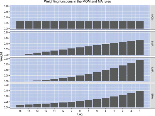
For the sake of illustration, figure 1 plots the shapes of the weighting functions for returns in the MOM, SMA, LMA, and EMA rules. In all rules, the size of the averaging window equals n = 15. The weights are normalized such that the sum of weights equals unity (that is, $\sum _i{\theta }_i=1$). Observe that in all but the MOM rule, the weighting function overweights the most recent returns.

Figure 1. The shapes of the weighting functions for returns in the MOM rule and MA rules. In all rules, the size of the averaging window equals n = 15. The weights are normalized such that the sum of weights equals unity. The return weights in the EMA rule are cut off at lag 15.

3. Data and popular lag lengths

We broaden the appeal and practical importance of our theoretical results by offering a number of illustrations and real-world examples. For this purpose, we calibrate our models to long-term historical data for the US stock market. The data used in our study are the monthly capital gain and total returns on the Standard and Poor's Composite stock price index, as well as the risk-free rate of return proxied by the T-bill rate. Our sample period begins in January 1857 and ends in December 2017. The data on the S&P Composite index come from two sources. The returns for the period from January 1857 to December 1925 are provided by William Schwert.⁵ The returns for the period from January 1926 to December 2017 are computed from the monthly closing prices of the S&P Composite index and corresponding dividend data provided by Amit Goyal.⁶ The T-bill rate for the period from January 1920 to December 2017 is also provided by Amit Goyal. Because there was no risk-free short-term debt prior to the 1920s, we estimate it in the same manner as in Welch and Goyal (2008) using the monthly data for the Commercial Paper Rates for New York. These data are available for the period from January 1857 to December 1971 from the National Bureau of Economic Research (NBER) Macrohistory database.⁷

The commonalities and differences between various trend-following rules analyzed in this paper are illustrated using the model parameters that encompass the actual characteristics of the monthly US stock market data. In particular, Section 7 of this paper documents, among other things, some key properties of actual stock market trends. Similarly, in our illustrations and real-world examples, we use averaging window sizes that encompass the most popular lag lengths in trend-following rules. Undeniably, the most popular of the MA rules is the SMA rule, where the most typical lag length equals 10 months. A number of empirical studies demonstrate that the performance of this rule is robust to the choice of lag length. Specifically, the SMA rule delivers good performance for lag lengths that span the range from 6 to 14 months (see Faber 2007, Kilgallen 2012, Neely et al. 2014). In the MOM rule, the most typical lag length is 12 months. However, Jegadeesh and Titman (1993) and Moskowitz et al. (2012) provide evidence that in equity markets, the momentum strategy is profitable over lag lengths that span the range from 6 to 12 months. Motivated by this evidence and actual characteristics of stock market trends, this paper uses lag lengths that span periods from 1 to 24 months. The numerical characteristics of trading rules with a window size of 10 months often serve as a benchmark for comparison in our numerical illustrations.

4. Return process

Weak-form market efficiency claims that past price movements cannot be used to predict future price movements. Effectively, this means that returns must follow a random walk, which rules out the notion that technical analysis has any value. In sharp contrast to this claim, there is a vast literature that demonstrates strong evidence of the profitability of trend-following rules (examples are Brock et al. 1992, Jegadeesh and Titman 1993, Faber 2007, Zhu and Zhou 2009, Gwilym et al. 2010, Kilgallen 2012, Moskowitz et al. 2012, Neely et al. 2014, Pätäri and Vilska 2014, Han et al. 2016, Faber 2017, Glabadanidis 2017).

For the trend-following strategies to be profitable, there must be price trends in real markets. A trend can be defined as price persistence, which is the tendency of a price to continue moving in its present direction. Price persistence means that returns are positively autocorrelated. In particular, if price continues moving upward (downward), a positive (negative) return tends to be followed again by a positive (negative) return. In a continuous-time setting, price persistence is typically modeled using the Ornstein-Uhlenbeck process for returns (see Zhu and Zhou 2009, Han et al. 2016, Ayed et al. 2017 among others). In discrete time, the price trend is commonly modeled by an AR(1) process, which is the discrete-time analogue of the continuous Ornstein-Uhlenbeck process (examples are Acar 1998, Lequeux 2005, Hong and Satchell 2015). In our paper, the return process incorporates higher order autoregressive lags that are often needed to capture the complex dynamics of real markets.

Specifically, we assume that the returns follow an autoregressive process of order p. This $AR\left(p\right)$ model is defined as: (6) $\begin{array}{rl}{X}_t& ={\phi }_1{X}_{t-1}+{\phi }_2{X}_{t-2}+\cdots +{\phi }_p{X}_{t-p}+{\epsilon }_t\\ & =\sum _{i=1}^p{\phi }_i{X}_{t-i}+{\epsilon }_t,\end{array}$(6) where p is the number of autoregressive terms, the coefficients $\{{\phi }_1,{\phi }_2,\dots ,{\phi }_p\}$ are the parameters of the model, $X_{t-i}$ is the return observed at time t−i, and ${\epsilon }_t$ is the noise term, which is an i.i.d. random process with zero mean and variance ${\sigma }_{\epsilon }^2$. That is, ${\epsilon }_t\sim iid(0,{\sigma }_{\epsilon }^2)$. We assume that the autoregressive coefficients ${\phi }_i$ satisfy the stationarity conditions. Note that we do not consider the drift term in the equation for $X_t$. This is because throughout this paper, we are interested in computing the correlation coefficients only, and the correlations are invariant to the addition of a constant term. In other words, the formulas for the correlation coefficients do not depend on the value of the drift term in the equation for $X_t$. Note that when p = 0, the returns follow a random walk without drift model $X_t={\epsilon }_t$.

By multiplying equation (6(6) $\begin{array}{rl}{X}_t& ={\phi }_1{X}_{t-1}+{\phi }_2{X}_{t-2}+\cdots +{\phi }_p{X}_{t-p}+{\epsilon }_t\\ & =\sum _{i=1}^p{\phi }_i{X}_{t-i}+{\epsilon }_t,\end{array}$(6) ) by $X_{t-k}$, taking expectations, and then dividing the resulting expression by the variance of $X_t$, we obtain the important recursive relationship for the autocorrelation coefficients of the $AR\left(p\right)$ process: (7) ${\rho }_k={\phi }_1{\rho }_{k-1}+{\phi }_2{\rho }_{k-2}+\cdots +{\phi }_p{\rho }_{k-p}.$(7) where ${\rho }_i$ denotes the autocorrelation between $X_t$ and $X_{t-i}$. Plugging $k=1,2,\dots ,p$ into equation (7(7) ${\rho }_k={\phi }_1{\rho }_{k-1}+{\phi }_2{\rho }_{k-2}+\cdots +{\phi }_p{\rho }_{k-p}.$(7) ) and using ${\rho }_0=1$ and ${\rho }_{-i}={\rho }_i$, we obtain the set of Yule-Walker linear equations. Given numerical values for $\{{\phi }_1,{\phi }_2,\dots ,{\phi }_p\}$, these linear equations can be solved to obtain numerical values for $\{{\rho }_1,{\rho }_2,\dots ,{\rho }_p\}$. Equation (7(7) ${\rho }_k={\phi }_1{\rho }_{k-1}+{\phi }_2{\rho }_{k-2}+\cdots +{\phi }_p{\rho }_{k-p}.$(7) ) can then be recursively used to obtain numerical values for ${\rho }_k$ for any k>p.

Since our goal is to model price trends, we need to choose numerical values for $\{{\phi }_1,{\phi }_2,\dots ,{\phi }_p\}$ that guarantee positive autocorrelation coefficients of the $AR\left(p\right)$ process. The following proposition, the proof of which is given in the Appendix, determines the condition under which the autocorrelation coefficients are positive.

Proposition 1

If all coefficients $\{{\phi }_1,{\phi }_2,\dots ,{\phi }_p\}$ of the $AR\left(p\right)$ process are positive, then all autocorrelation coefficients ${\rho }_k$ are also positive.

The sum of the autoregressive coefficients, $\alpha =\sum _{i=1}^p{\phi }_i$, can be used as a measure of persistence. This measure was proposed by Andrews and Chen (1994) and subsequently by Marques (2005). Specifically, Marques (2005) begins by observing that every autoregressive process $AR\left(p\right)$ is, in fact, a mean-reverting process. The speed of mean reversion is inversely proportional to α. In particular, the larger the numerical value of α is, the slower the reversion to the long-run mean and, hence, the stronger the price trend. Consequently, the sum of the autoregressive coefficients can be used to measure persistence.

Note that if all coefficients $\{{\phi }_1,{\phi }_2,\dots ,{\phi }_p\}$ of the $AR\left(p\right)$ process are nonnegative, then increasing the numerical value of some ${\phi }_i$ or increasing the order p increases the persistence of the $AR\left(p\right)$ process. Consequently, the choices for p and ${\phi }_i$ influence the persistence and, hence, the duration of the price trend. Ceteris paribus, increasing either the number of autoregressive terms or the values of the autoregressive coefficients makes the price trend stronger and long lasting. The following proposition, the proof of which is given in the Appendix, formalizes this idea.

Proposition 2

If all coefficients $\{{\phi }_1,{\phi }_2,\dots ,{\phi }_p\}$ of the $AR\left(p\right)$ process are nonnegative, then all autocorrelation coefficients ${\rho }_k$ increase as α, the measure of persistence of the $AR\left(p\right)$ process, increases.

5. Similarity between trend-following indicators

5.1. Theoretical results

The goal of this section is to measure the similarity between two generally different trading indicators $I_t\left(n\right)$ and $J_t\left(m\right)$. The trading indicator $J_t\left(m\right)$ is computed in a manner similar to that of $I_t\left(n\right)$. Formally, the computation of trading indicators $I_t\left(n\right)$ and $J_t\left(m\right)$ is given by $I_t\left(n\right)=\sum _{i=0}^{n-1}{\theta }_{I,i}{X}_{t-i}{J}_t\left(m\right)=\sum _{i=0}^{m-1}{\theta }_{J,i}{X}_{t-i}.$ The difference between these two trading indicators consists of using different numbers of past returns (generally $n\ne m$) and/or different weighting functions for returns. In vector notation, the weighting functions in each trading indicator are given by ${\mathit{\theta }}_{I,n}^{\mathrm{\prime }}=[{\theta }_{I,0},{\theta }_{I,1},\dots ,{\theta }_{I,n-1}],{\mathit{\theta }}_{J,m}^{\mathrm{\prime }}=[{\theta }_{J,0},{\theta }_{J,1},\dots ,{\theta }_{J,m-1}],$ where ${\mathit{a}}^{\mathbf{\prime }}$ denotes the transpose of vector $\mathit{a}$.

Since the trading indicator given by (3(3) $I_t\left(n\right)=\sum _{i=0}^{n-2}{\theta }_i{X}_{t-i},$(3) ) is a linear function of past random returns and the trading signal is invariant to the scaling of past returns (see equation (4(4) $\mathrm{s}\mathrm{g}\mathrm{n}\left(c\times I_t\left(n\right)\right)=\mathrm{s}\mathrm{g}\mathrm{n}\left(I_t\left(n\right)\right),$(4) )), as a measure of similarity between two trading indicators, it is natural to use the correlation coefficient. Consequently, we are interested in computing the following linear correlation coefficient (a.k.a. Pearson correlation coefficient) $Cor\left(I_t\right(n),J_t(m\left)\right)$. This correlation coefficient is scale and location invariant. For example, the correlation coefficient is the same for all equivalent trading indicators. Specifically, for an equivalent trading indicator $c\times I_t\left(n\right)$, which is obtained by scaling by c>0 the weights ${\mathit{\theta }}_{I,n}$ of indicator $I_t\left(n\right)$, the following property is satisfied: $Cor(c\times I_t(n),J_t(m\left)\right)=Cor\left(I_t\right(n),J_t(m\left)\right).$ Similarly, this correlation coefficient does not depend on the value of the drift term in the equation for the return process, as the drift value only changes the location of $I_t\left(n\right)$ and $J_t\left(m\right)$.

Proposition 3

When the returns follow the $AR\left(p\right)$ process, the correlation coefficient between two trading indicators $I_t\left(n\right)$ and $J_t\left(m\right)$ is given by (8) $Cor\left(I_t\right(n),J_t(m\left)\right)=\frac{{\mathit{\theta }}_{I,n}^{\mathrm{\prime }}{\mathit{P}}_{n,m}{\mathit{\theta }}_{J,m}}{\sqrt{{\mathit{\theta }}_{I,n}^{\mathrm{\prime }}{\mathit{P}}_{n,n}{\mathit{\theta }}_{I,n}}\sqrt{{\mathit{\theta }}_{J,m}^{\mathrm{\prime }}{\mathit{P}}_{m,m}{\mathit{\theta }}_{J,m}}},$(8) where ${\mathit{P}}_{n,m}$ is the $n\times m$ matrix given by (9) ${\mathit{P}}_{n,m}=\left[\begin{array}{ccccc}1& {\rho }_1& {\rho }_2& \dots & {\rho }_{m-1}\\ {\rho }_1& 1& {\rho }_1& \dots & {\rho }_{m-2}\\ {\rho }_2& {\rho }_1& 1& \dots & {\rho }_{m-3}\\ ⋮& ⋮& ⋮& \ddots & ⋮\\ {\rho }_{n-1}& {\rho }_{n-2}& {\rho }_{n-3}& \dots & {\rho }_{|m-n|}\end{array}\right],$(9) where ${\rho }_i$ is the autocorrelation of order i of the $AR\left(p\right)$ process for returns.

The proof is given in the Appendix.

Remark 1

When the returns follow the $AR\left(1\right)$ process, the autocorrelation of order i is given by ${\rho }_i={\phi }_1^i$. In this case, matrix ${\mathit{P}}_{n,m}$ becomes (10) ${\mathit{P}}_{n,m}=\left[\begin{array}{ccccc}1& {\phi }_1& {\phi }_1^2& \dots & {\phi }_1^{m-1}\\ {\phi }_1& 1& {\phi }_1& \dots & {\phi }_1^{m-2}\\ {\phi }_1^2& {\phi }_1& 1& \dots & {\phi }_1^{m-3}\\ ⋮& ⋮& ⋮& \ddots & ⋮\\ {\phi }_1^{n-1}& {\phi }_1^{n-2}& {\phi }_1^{n-3}& \dots & {\phi }_1^{|m-n|}\end{array}\right].$(10)

Remark 2

When the returns follow a random walk, equation (8(8) $Cor\left(I_t\right(n),J_t(m\left)\right)=\frac{{\mathit{\theta }}_{I,n}^{\mathrm{\prime }}{\mathit{P}}_{n,m}{\mathit{\theta }}_{J,m}}{\sqrt{{\mathit{\theta }}_{I,n}^{\mathrm{\prime }}{\mathit{P}}_{n,n}{\mathit{\theta }}_{I,n}}\sqrt{{\mathit{\theta }}_{J,m}^{\mathrm{\prime }}{\mathit{P}}_{m,m}{\mathit{\theta }}_{J,m}}},$(8) ) for the correlation coefficient reduces to (by setting ${\rho }_i=0$ for all $i\ge 1$) (11) $Cor\left(I_t\right(n),J_t(m\left)\right)=\frac{{\mathit{\theta }}_{I,k}^{\mathrm{\prime }}{\mathit{\theta }}_{J,k}}{\parallel {\mathit{\theta }}_{I,n}\parallel \parallel {\mathit{\theta }}_{J,m}\parallel },$(11) where $\parallel \mathit{a}\parallel =\sqrt{{\mathit{a}}^{\mathrm{\prime }}\cdot \mathit{a}}$ and $k=min(n,m)$. For example, ${\mathit{\theta }}_{I,k}$ is a vector that consists of the first k elements of vector ${\mathit{\theta }}_{I,n}$.

Remark 3

Note that the correlation coefficient $Cor\left(I_t\right(n),J_t(m\left)\right)$ does not depend on the amount of noise in the return process. In particular, $Cor\left(I_t\right(n),J_t(m\left)\right)$ depends neither on ${\sigma }_{\epsilon }^2$ nor on ${\sigma }_x^2$, where the latter is the variance of $X_t$.

Remark 4

Regardless of the order p of the $AR\left(p\right)$ process for returns $Cor\left(I_t\right(n),I_t(n\left)\right)=1.$ This is because $I_t\left(n\right)$ is a random variable, and any random variable is perfectly positively correlated with itself.

Proposition 4

Given that all elements of ${\mathit{\theta }}_{I,n}$ and ${\mathit{\theta }}_{J,m}$ are positive, if all coefficients $\{{\phi }_1,{\phi }_2,\dots ,{\phi }_p\}$ of the $AR\left(p\right)$ process are nonnegative, then the correlation coefficient $Cor\left(I_t\right(n),J_t(m\left)\right)$ is positive.

The proof is given in the Appendix.

Remark 5

If the conditions of Proposition 4 are satisfied, then the obvious conclusion is that $0<Cor\left(I_t\right(n),J_t(m\left)\right)\le 1.$ That is, the trading indicators of all rules are positively correlated. It is worth emphasizing that the correlation between trading indicators is positive even if the returns follow a random walk. That is, trading indicators are positively correlated even in the absence of return predictability.

Proposition 5

If all coefficients $\{{\phi }_1,{\phi }_2,\dots ,{\phi }_p\}$ of the $AR\left(p\right)$ process are nonnegative and $Cor\left(I_t\right(n),J_t(m\left)\right)<1,$ then the correlation coefficient $Cor\left(I_t\right(n),J_t(m\left)\right)$ increases with increasing persistence of the $AR\left(p\right)$ process.

The proof is given in the Appendix.

Remark 6

Note that Proposition 5 states that the similarity between the rules increases when the price trend strengthens. In other words, the stronger the price trend is, the greater the similarity between trading indicators of various trend-following rules.

5.2. Numerical illustrations

The goal of this section is to illustrate the similarity between two trading indicators. First, we study the similarity between two trading indicators that belong to the same rule. These indicators employ the same weighting function for returns but are computed using different sizes of the averaging window. In other words, we study the correlation coefficient $Cor\left(I_t\right(n),I_t(m\left)\right)$.

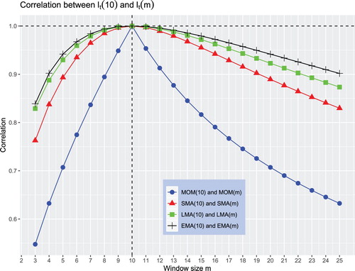
We begin with the case in which the returns follow a random walk. Figure 2 plots the correlation coefficient $Cor\left(I_t\right(n),I_t(m\left)\right)$ for the MOM and all MA rules⁸ when n = 10 and $m\in [2,25]$. The correlation plots in this figure suggest the following observations. The first observation is that, in accordance with Remark 4, the correlation $Cor\left(I_t\right(n),I_t(m\left)\right)=1$ for all rules when n = m. The second observation is that when the size of the averaging window m diverges from n in any direction, the correlation $Cor\left(I_t\right(n),I_t(m\left)\right)$ decreases. This correlation decreases much faster for the MOM rule than for any MA rule. Consequently, for two different sizes of the averaging window, the trading indicators of the MA rules are more similar than those of the MOM rule. In other words, the trading indicator of the MA rules exhibits robustness to the change in the size of the averaging window. In particular, as opposed to the MOM rule, changing the size of the averaging window in an MA rule has little influence on the generation of a trading signal. Among the MA rules, the EMA rule exhibits the greatest robustness. In our illustration, even under a random walk, the correlation between trading indicators of two EMA rules exceeds 80%.

Figure 2. Similarity between $I_t\left(10\right)$ and $I_t\left(m\right)$ when returns follow a random walk.

Why is the trading indicator of an MA rule more robust to a change in the size of the averaging window than the trading indicator of the MOM rule? This is because an MA rule underweights (overweights) the most distant (recent) returns. The consequence of reducing the effect of the most distant returns in the computation of a trading indicator can be illustrated as follows. Under the assumption that m>n, the computation of trading indicator $I_t\left(m\right)$ can be rewritten as $I_t\left(m\right)=\sum _{i=0}^{m-1}{\theta }_i^m{X}_{t-i}=\sum _{i=0}^{n-1}{\theta }_i^m{X}_{t-i}+\sum _{i=n}^{m-1}{\theta }_i^m{X}_{t-i},$ where the notation ${\theta }_i^m$ denotes the return weights when the size of the averaging window equals m. Note that for any MA rule, ${\theta }_i^n\ne {\theta }_i^m$. Only for the MOM rule does ${\theta }_i^n={\theta }_i^m=1$.

In our notation, the correlation coefficient is given by $\begin{array}{rl}& Cor\left(I_t\right(n),I_t(m\left)\right)\\ & =Cor\left(\sum _{i=0}^{n-1}{\theta }_i^n{X}_{t-i},\sum _{i=0}^{n-1}{\theta }_i^m{X}_{t-i}+\sum _{i=n}^{m-1}{\theta }_i^m{X}_{t-i}\right).\end{array}$ With this representation, it becomes apparent that the dissimilarity between $I_t\left(n\right)$ and $I_t\left(m\right)$ comes from the term $\sum _{i=n}^{m-1}{\theta }_i^m{X}_{t-i}$, which is independent of $I_t\left(n\right)$ under a random walk. This representation also suggests that the dissimilarity between $I_t\left(n\right)$ and $I_t\left(m\right)$ can be reduced by decreasing the weights ${\theta }_i^m$ for $i\ge n$. In other words, the similarity between $I_t\left(n\right)$ and $I_t\left(m\right)$ can be increased by reducing (increasing) the weights of the most distant (recent) returns. This is precisely what is done in all MA rules.

From Proposition 5, we know that the similarity between the rules increases when the return process becomes more persistent. To illustrate this property, we compute the correlation coefficient $Cor\left(I_t\right(n),I_t(m\left)\right)$ for orders $p\in \{0,1,2,3\}$ in the $AR\left(p\right)$ process for returns. For simplicity, we assume that, regardless of the number of autoregressive terms p, all ${\phi }_i$ coefficients are alike and equal 0.3. For two selected rules, MOM and EMA, figure 3 plots the correlation coefficient $Cor\left(I_t\right(n),I_t(m\left)\right)$ for different orders of the $AR\left(p\right)$ process. As before, we fix n = 10 and vary $m\in [2,25]$. As expected, the correlation plots in figure 3 show that the similarity between the same trading indicator computed using different sizes of the averaging window increases when the order of the $AR\left(p\right)$ process increases.

Figure 3. Similarity between $I_t\left(10\right)$ and $I_t\left(m\right)$ when returns follow the $AR\left(p\right)$ process where $p\in \{0,1,2,3\}$. Note that $AR\left(0\right)$ is a random walk (RW) process. Regardless of the number of autoregressive terms p, ${\phi }_i=0.3$ for all $i\le p$.

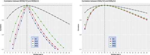
When the persistence of the return process increases, the similarity between two MOM rules increases more rapidly than the similarity between two EMA rules. However, our experiments suggest that, regardless of the degree of persistence of the return process, the similarity between two MA rules is always higher than the similarity between two MOM rules with corresponding sizes of the averaging window.

Now, we turn to studying the similarity between two different trading indicators. That is, we study the correlation coefficient $Cor\left(I_t\right(n),J_t(m\left)\right)$. We begin with the case in which the returns follow a random walk. Figure 4 plots the correlation coefficients between the trading indicators of two different rules when n = 10 and $m\in [2,25]$. In particular, it plots $Cor\left(I_t\right(10),J_t(m\left)\right)$ when I is either the MOM or SMA rule and J is a rule that is different from I. The correlation plots in this figure suggest the following observations. First, as m increases, the correlation between two trading indicators first increases, attains a maximum, and then decreases. Even under a random walk, the maximum correlation between two trading indicators is high and exceeds 90%. The maximum is attained at $m\ne n$. Second, the similarity between two different MA rules is generally greater than the similarity between the MOM and an MA rule. The maximum correlation between two different MA rules is higher than the maximum correlation between the MOM and an MA rule. This observation is not surprising given that, qualitatively, the weighting functions of the MA rules share many similarities (see figure 1). In contrast, the weighting function of an MA rule is clearly different from that of the MOM rule. As a result of the considerable similarities between the weighting functions of two MA rules, the maximum correlation coefficient between trading indicators of two MA rules approaches 100% even under a random walk.

Figure 4. Similarity between $I_t\left(10\right)$ and $J_t\left(m\right)$ when returns follow a random walk.

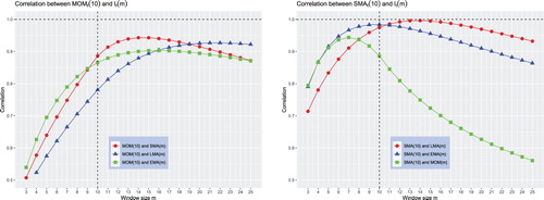
Finally, in this section, we illustrate the similarity between two different trading indicators when the persistence of the $AR\left(p\right)$ process increases. As before, we vary $p\in \{0,1,2,3\}$ and assume that, regardless of the number of autoregressive terms p, all ${\phi }_i$ coefficients are alike and equal 0.3. Figure 5 plots the correlation coefficients between different trading rules. In particular, the left panel in this figure plots $Cor\left(MO{M}_t\right(10),SM{A}_t(m\left)\right)$, whereas the right panel plots $Cor\left(SM{A}_t\right(10),EM{A}_t(m\left)\right)$. In accordance with Proposition 5, the similarity between two different trading indicators increases when the order of the $AR\left(p\right)$ process increases.

Figure 5. Similarity between $I_t\left(10\right)$ and $J_t\left(m\right)$ when returns follow the $AR\left(p\right)$ process where $p\in \{0,1,2,3\}$. Note that $AR\left(0\right)$ is a random walk (RW) process. Regardless of the number of autoregressive terms p, ${\phi }_i=0.3$ for all $i\le p$.

6. Similarity between trading indicator and future return

6.1. Theoretical results

The goal of this section is to measure the similarity between the value of a trading indicator $I_t\left(n\right)$ and the next period return $X_{t+1}$. Recall that the technical indicator is computed at time t and translated into a trading signal for the subsequent period until time t + 1. In essence, a trading indicator is nothing else than a linear forecasting equation that is used to predict the next period return. The forecast accuracy of such a predictor is commonly measured by the mean squared error between the forecast value and the next period return. However, since the trading signal is invariant to the scaling of past returns (see equation (4(4) $\mathrm{s}\mathrm{g}\mathrm{n}\left(c\times I_t\left(n\right)\right)=\mathrm{s}\mathrm{g}\mathrm{n}\left(I_t\left(n\right)\right),$(4) )), we measure the similarity between the trading indicator and the future return by the correlation coefficient $Cor(X_{t+1},I_t(n\left)\right)$.

Proposition 6

When the returns follow the $AR\left(p\right)$ process, the correlation coefficient between the trading indicators $I_t\left(n\right)$ and the next period return $X_{t+1}$ is given by (12) $Cor(X_{t+1},I_t(n\left)\right)=\frac{{\mathit{\theta }}_n^{\mathrm{\prime }}{\mathit{P}}_{n,p}{\mathit{\phi }}_p}{\sqrt{{\mathit{\theta }}_n^{\mathrm{\prime }}{\mathit{P}}_{n,n}{\mathit{\theta }}_n}},$(12) where ${\mathit{\phi }}_p^{\mathrm{\prime }}=[{\phi }_1,{\phi }_2,\dots ,{\phi }_p]$ is the vector of autoregressive coefficients of $X_t,{\mathit{\theta }}_n^{\mathrm{\prime }}=[{\theta }_0,{\theta }_1,\dots ,{\theta }_{n-1}]$ is the vector that contains the elements of the weighting function of $I_t\left(n\right)$, and matrix ${\mathit{P}}_{n,p}$ is given by (9(9) ${\mathit{P}}_{n,m}=\left[\begin{array}{ccccc}1& {\rho }_1& {\rho }_2& \dots & {\rho }_{m-1}\\ {\rho }_1& 1& {\rho }_1& \dots & {\rho }_{m-2}\\ {\rho }_2& {\rho }_1& 1& \dots & {\rho }_{m-3}\\ ⋮& ⋮& ⋮& \ddots & ⋮\\ {\rho }_{n-1}& {\rho }_{n-2}& {\rho }_{n-3}& \dots & {\rho }_{|m-n|}\end{array}\right],$(9) ).

The proof is given in the Appendix.

Remark 7

Note that the Yule-Walker equations can be expressed in matrix form as (see, for example, Box et al. 2016, p. 57) (13) ${\mathit{P}}_{n,p}{\mathit{\phi }}_p={\mathit{\rho }}_n,$(13) where ${\mathit{\rho }}_n^{\mathrm{\prime }}=[{\rho }_1,{\rho }_2,\dots ,{\rho }_n]$ is the vector that contains the first n autocorrelations of the $AR\left(p\right)$ process for returns. Thus, an alternative expression for the correlation between the trading indicator and the next period return is given by (14) $Cor(X_{t+1},I_t(n\left)\right)=\frac{{\mathit{\theta }}_n^{\mathrm{\prime }}{\mathit{\rho }}_n}{\sqrt{{\mathit{\theta }}_n^{\mathrm{\prime }}{\mathit{P}}_{n,n}{\mathit{\theta }}_n}}.$(14)

Remark 8

It is worth observing that if the returns follow a random walk (in this case, ${\mathit{\phi }}_p=\mathbf{0}$ and ${\mathit{\rho }}_n=\mathbf{0}$), the correlation $Cor(X_{t+1},I_t(n\left)\right)=0$. That is, when the returns follow a random walk, no trading indicator can predict the next period return. Conversely, a trading indicator is able to predict the future return only if there is some persistence in the return process.

Proposition 7

If all coefficients $\{{\phi }_1,{\phi }_2,\dots ,{\phi }_p\}$ of the $AR\left(p\right)$ process are nonnegative, then the correlation coefficient $Cor(X_{t+1},I_t(n\left)\right)$ increases with increasing persistence of the $AR\left(p\right)$ process.

The proof is given in the Appendix.

Remark 9

Proposition 7 implies that the stronger the trend is, the better the forecast accuracy of any trend-following indicator.

The natural question to ask is how to choose the weights ${\theta }_i$ in a trading rule to maximize the correlation between the trading indicator and future returns. The following proposition derives the weights of the optimal trading rule.

Proposition 8

The trading rule that maximizes $Cor(X_{t+1},I_t(n\left)\right)$ is given by (15) $I_t\left(p\right)=\sum _{i=0}^{p-1}\left(c\times {\phi }_{i+1}\right)X_{t-i},$(15) where c is any positive real number.

The proof is given in the Appendix.

Remark 10

The result derived in Proposition 8 is not surprising and can be obtained via the following shortcut. In particular, in the time-series literature, it is known that the ‘best linear predictor’ of the $AR\left(p\right)$ process has the same coefficients as the autoregressive coefficients in the $AR\left(p\right)$ process (see, for example, Box et al. 2016, p. 131). Consequently, the trading indicator that provides the best forecast accuracy has weights ${\theta }_i={\phi }_{i+1}$ for $i\in [0,p-1]$ and ${\theta }_i=0$ for $i\ge p$. This ‘best linear predictor’ has the least mean squared error between the forecast value and the future return. It is easy to deduce that the ‘best linear predictor’ also has the highest correlation with the future value of the $AR\left(p\right)$ process. However, since our goal is to maximize the correlation coefficient and it is scale invariant, we can rescale the weights of the ‘best linear predictor’ without changing the correlation.

Remark 11

The maximum possible correlation between the trading indicator and the next period return is given by (16) $\underset{{\mathit{\theta }}_n}{max}Cor(X_{t+1},I_t(n\left)\right)=\sqrt{{\mathit{\phi }}_p^{\mathrm{\prime }}{\mathit{\rho }}_p}.$(16) This result can be easily obtained by inserting $c\times {\mathit{\phi }}_p$ instead of ${\mathit{\theta }}_n$ into equation (14(14) $Cor(X_{t+1},I_t(n\left)\right)=\frac{{\mathit{\theta }}_n^{\mathrm{\prime }}{\mathit{\rho }}_n}{\sqrt{{\mathit{\theta }}_n^{\mathrm{\prime }}{\mathit{P}}_{n,n}{\mathit{\theta }}_n}}.$(14) ) and using the result stated by equation (13(13) ${\mathit{P}}_{n,p}{\mathit{\phi }}_p={\mathit{\rho }}_n,$(13) ).

For example, if the returns follow the $AR\left(1\right)$ process with ${\phi }_1>0$, the trading rule that maximizes the correlation between the trading indicator and future returns is given by $I_t\left(1\right)=(c\times {\phi }_1)X_t$. A convenient choice in this case is to use $c=1/{\phi }_1$. This choice results in $I_t\left(1\right)=MO{M}_t\left(1\right)$. That is, if the returns follow the $AR\left(1\right)$ process, the best trading indicator is given by $MO{M}_t\left(1\right)$.⁹ With this choice, the correlation between the trading indicator and future returns amounts to $Cor(X_{t+1},MO{M}_t(1\left)\right)={\phi }_1$. As another example, suppose that the returns follow the $AR\left(2\right)$ process with ${\phi }_2={\phi }_1$. It can be easily deduced that in this case, the best trading indicator is given by $MO{M}_t\left(2\right)$. Since according to Proposition 7 the similarity between the trading indicator and future returns increases when the persistence increases, in our example, $Cor(X_{t+1},MO{M}_t(2\left)\right)>{\phi }_1$.

Remark 12

Note that the trading indicator is optimal if its weights ${\theta }_i$ represent rescaled versions of the autoregressive coefficients ${\phi }_i$ of the $AR\left(p\right)$ process. Consequently, the MOM rule is optimal when all autoregressive coefficients are equal. The SMA (EMA) rule is optimal when the autoregressive coefficients are linearly (exponentially) decreasing.

However, what if none of the available trading rules is optimal given some particular $AR\left(p\right)$ process for returns? In this case, one can find the size of the averaging window $n^{\ast }$ in a trading indicator that maximizes the correlation with the future return. That is, one can solve the following problem: (17) $Cor(X_{t+1},I_t(n^{\ast }\left)\right)=\underset{n}{max}Cor(X_{t+1},I_t(n\left)\right).$(17) It is very difficult, if ever possible, to analytically find the size of the averaging window $n^{\ast }$ in a trading rule that maximizes the correlation. However, it is trivial to find $n^{\ast }$ by using numerical methods. By performing this task for every trading rule, one can select the rule that has the highest correlation with the future return.

6.2. Numerical illustrations

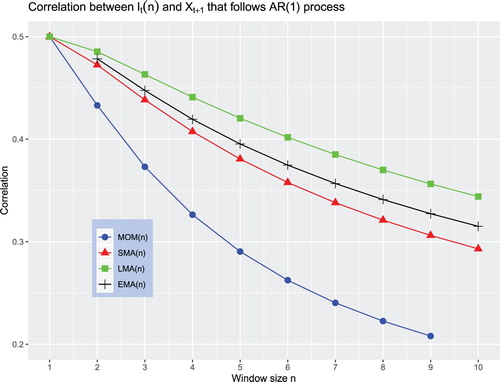
The goal of this subsection is to illustrate the similarity between the trading indicator and the next period return. First, we assume that $X_t$ follows the $AR\left(1\right)$ process with ${\phi }_1=0.5$. Figure 6 plots the correlation $Cor(X_{t+1},I_t(n\left)\right)$ for different trading rules; the size of the averaging window n is varied from 1 to 10. Note that the optimal trading indicator in this case is $I_t\left(1\right)=X_t$, which provides the highest possible correlation, which amounts to ${\phi }_1$, with the future return. This trading indicator can be realized by any trading rule except the EMA rule because the trading indicator in the EMA rule is not defined for n = 1 (in this case, $\lambda =0$). The main conclusion that can be drawn from figure 6 is that as n increases, the correlation $Cor(X_{t+1},I_t(n\left)\right)$ decreases for all rules. However, the correlation between $Cor(X_{t+1},I_t(n\left)\right)$ decreases substantially faster for the MOM rule than for any MA rule. This result is not surprising given that all MA rules overweight the most recent returns. The LMA rule provides the correlation that is the most robust to the change in the size of the averaging window.

Figure 6. The correlation $Cor(X_{t+1},I_t(n\left)\right)$ when $X_t$ follows the AR(1) process with ${\phi }_1=0.5$.

Second, we assume that $X_t$ follows the $AR\left(5\right)$ process. We consider two cases. In the first case, the coefficients of the autoregressive process are all alike ${\mathit{\phi }}_{\mathbf{5}}^{\mathbf{\prime }}=[0.15,0.15,0.15,0.15,0.15]$. In the second case, the coefficients decrease linearly ${\mathit{\phi }}_{\mathbf{5}}^{\mathbf{\prime }}=[0.25,0.20,0.15,0.10,0.05]$. We know that in the first case, the best trading rule is MOM(5), whereas in the second case, the best trading rule is SMA(5). These rules provide the highest correlation between the trading indicator and the next period return in each case. However, what about the correlation coefficient for the other rules and other sizes of the averaging window?

Figure 7, Panel A, plots the correlation $Cor(X_{t+1},I_t(n\left)\right)$ against n when returns follow the $AR\left(5\right)$ process where all autoregressive coefficients are alike; the table in Panel C reports the maximum possible correlation $Cor(X_{t+1},I_t(n^{\ast }\left)\right)$ for each rule. Our first observation is that for all rules, as n increases, the correlation first increases, attains its maximum, and then decreases. Our second observation is that when $n\le 5$, the MOM rule provides the correlation $Cor(X_{t+1},I_t(n\left)\right)$, which is larger than that for any MA rule. However, as the size of the averaging window increases beyond 5, the correlation between $MO{M}_t\left(n\right)$ and $X_{t+1}$ decreases rather quickly; for n>6, the correlation between any MA rule and the future return is higher than that between the MOM rule and the future return. Even though the correlation between any rule and the future return eventually decreases as the size of the averaging window increases, the MA rules provide substantially higher correlation than that provided by the MOM rule.

Figure 7. Correlation between $I_t\left(n\right)$ and $X_{t+1}$ when returns follow the $AR\left(5\right)$ process. The graph in Panel A plots $Cor(X_{t+1},I_t(n\left)\right)$, whereas the table in Panel C reports $Cor(X_{t+1},I_t(n^{\ast }\left)\right)$ when all autocorrelation coefficients are alike. Specifically, when ${\mathit{\phi }}_{\mathbf{5}}^{\mathbf{\prime }}=[0.15,0.15,0.15,0.15,0.15]$. The graph in Panel B plots $Cor(X_{t+1},I_t(n\left)\right)$, whereas the table in Panel C reports $Cor(X_{t+1},I_t(n^{\ast }\left)\right)$ when the autocorrelation coefficients are linearly decreasing, in particular, when ${\mathit{\phi }}_{\mathbf{5}}^{\mathbf{\prime }}=[0.25,0.20,0.15,0.10,0.05]$.

Our third observation is related to the correlation $Cor(X_{t+1},I_t(n^{\ast }\left)\right)$ reported in the table in Panel C. Even though an MA rule is not optimal when all autoregressive coefficients are alike, one can always find the $n^{\ast }$ that provides the correlation (between the trading indicator and future return) that is only marginally less than the correlation provided by the MOM(5) rule. For example, the correlation between the MOM(5) and the future return amounts to 0.530. Instead of the MOM(5) rule, one can use the SMA(7) rule that provides a correlation of 0.523, which is only approximately 1% smaller than the maximum possible correlation. The LMA(10) rule and the EMA(7) are also almost as good as the MOM(5) rule.

Figure 7, Panel B, plots the correlation $Cor(X_{t+1},I_t(n\left)\right)$ when returns follow the $AR\left(5\right)$ process where the autoregressive coefficients are linearly decreasing; the table in Panel D reports $Cor(X_{t+1},I_t(n^{\ast }\left)\right)$. The results for the first and second cases share numerous similarities but differ in choice of the best trading indicator. As in the first case, for all rules, as n increases, the correlation first increases, attains its maximum, and then decreases. In the same manner as in the first case, after attaining its maximum, the correlation decreases faster for the MOM rule. Again, the maximum possible correlations between a trading indicator and future return differ only marginally among the various rules. Specifically, the maximum possible correlation is provided by the SMA(5) rule and equals 0.577. Replacing the SMA(5) rule with the MOM(4) rule reduces the correlation to only 0.569; the reduction amounts to approximately 1%.

The main conclusions that can be drawn from figure 7 are as follows. In any trading indicator $I_t\left(n\right)$, one can find the size of the averaging window $n^{\ast }$ that maximizes the correlation between the indicator and future returns. Our numerical illustrations suggest that this correlation is only marginally smaller than the highest possible correlation. The trading rules differ mainly in the robustness of the correlation to the change in the size of the averaging window. As the size of the averaging window n in a trading rule diverges from $n^{\ast }$ in any direction, the correlation decreases. The decrease is generally larger for the MOM rule than for any MA rule. When the size of the averaging window n is substantially smaller than the order p of the $AR\left(p\right)$ process for returns, $n\ll p$, the trading indicator of the MOM rule might have a small advantage over the MA rules in terms of a higher correlation with the future return. However, the trading indicators of all MA rules provide a significantly higher similarity (compared to that of the MOM rule) with the future return when $n\gg p$. The latter result appears naturally as a consequence of overweighting the most recent returns in the computations of trading indicators of the MA rules.

7. Trend following under uncertain market dynamics

When the parameters of the $AR\left(p\right)$ process for returns are known, the trader can always find the optimal size of the averaging window $n^{\ast }$ in any trend-following rule that maximizes the correlation between the trading indicator and future returns. The results reported in the previous section suggest that all trend-following rules are nearly equally good and provide correlation (between the trading indicator and future returns) that is close to the maximum possible correlation. Given this fact, the empirical performance of all trend-following rules should be nearly identical. However, many empirical studies find that the SMA rule performs better than the MOM rule (see, among others, Neely et al. 2014, Zakamulin 2014, He and Li 2015, Marshall et al. 2017). The goal of this section is to suggest and develop a well-motivated hypothesis about uncertain market dynamics. We show that our hypothesis, coupled with our analytical results on the similarity between two trading indicators and the similarity between a trading indicator and future returns, has far-reaching practical implications and is able to explain a number of empirical observations. Among other things, our hypothesis explains why the performance of the MA rule is better, on average, than the performance of the MOM rule.

7.1. Motivation

Stock return predictability is a very intriguing but very controversial topic in the finance literature. The typical linear predictive regression that is used by researchers to predict the next period return is given by (18) $X_{t+1}={\text{β}}_0+{\text{β}}_1{Z}_t+{\epsilon }_t,$(18) where ${\text{β}}_0$ and ${\text{β}}_1$ are regression coefficients, $Z_t$ is a predictor variable observed at time t, and ${\epsilon }_t$ is a disturbance term. The standard predictor variables that are used in linear regression (18(18) $X_{t+1}={\text{β}}_0+{\text{β}}_1{Z}_t+{\epsilon }_t,$(18) ) are the past stock return, the stock dividend yield, the earnings yield, the default spread,¹⁰ the term premium,¹¹ the T-bill rate, and the inflation rate (see, among others, Fama 1981, Keim and Stambaugh 1986, Campbell 1987, Campbell and Shiller 1988, Fama and French 1989, Fama 1990, Jegadeesh 1991).

The evidence of return predictability was established using in-sample tests. However, as convincingly demonstrated by Welch and Goyal (2008), the evidence of out-of-sample predictability is very weak and almost nonexistent. The problem seems to lie in the instability of the regression coefficients in equation (18(18) $X_{t+1}={\text{β}}_0+{\text{β}}_1{Z}_t+{\epsilon }_t,$(18) ). In particular, the assumption of constant regression coefficients in linear return regression (18(18) $X_{t+1}={\text{β}}_0+{\text{β}}_1{Z}_t+{\epsilon }_t,$(18) ) has been challenged in numerous studies such as Paye and Timmermann (2006), Rapach and Wohar (2006), Chen and Hong (2012), Dangl and Halling (2012), and Johannes et al. (2014). All these studies find strong statistical evidence that this assumption is empirically rejected for US stock returns using standard predictor variables.

Motivated by the evidence of time-variation in the regression coefficients of predictive equation (18(18) $X_{t+1}={\text{β}}_0+{\text{β}}_1{Z}_t+{\epsilon }_t,$(18) ), we conjecture that the empirical returns follow the $AR\left(p\right)$ process where both the order of the process p and the autoregressive coefficients ${\phi }_i$ vary over time. Consequently, since in the optimal trading indicator, the size of the averaging window equals the order of the autoregressive process, n = p, and the past return weights equal the rescaled autoregressive coefficients, ${\theta }_i=c\times {\phi }_{i+1}$, under our conjecture, the parameters of the optimal trading indicator also vary over time.

Our conjecture is able to explain the major controversy among traders regarding the optimal size of the averaging window in a trading rule. For instance, for the most popular SMA rule, the recommended size varies from 10 to 200 days (see Brock et al. 1992, Sullivan et al. 1999, Okunev and White 2003, Kirkpatrick and Dahlquist 2010). Apparently, there are substantial variations in the recommended size of the averaging window in a trading rule. The natural question to ask is what is the reason for this controversy? Our explanation is as follows. Typically, traders conduct backtests of a trading rule to find the optimal size of the averaging window. In such a backtest, traders use historical returns in the recent past; often, a historical sample of past returns covers a period from 5 to 10 years. If our conjecture is true and the backtests are conducted at different times, then traders obtain different estimates for the optimal size of the averaging window since the order of the autoregressive process for returns varies over time.

Our conjecture can be supported by the following simple empirical study. The goal of this study is to find the optimal size of the averaging window $n^{\ast }$ in the MOM and SMA rules over a rolling period of N months and demonstrate that $n^{\ast }$ varies over time. The optimal size of the averaging window in each rule is found using the backtesting methodology. The methodology is illustrated by means of using the $MOM\left(n\right)$ rule. Specifically, given the size of the averaging window n in the $MOM\left(n\right)$ rule, we simulate the excess returns¹² to the long-only trend-following strategy over a given historical subsample $(r_t^n,r_{t+1}^n,\dots ,r_{t+N}^n)$ that starts at time t. The optimal size of the averaging window $n_t^{\ast }$ is found by maximizing the risk-adjusted performance of the $MOM\left(n\right)$ strategy. Formally, $n_t^{\ast }=\arg \underset{n\in [n^{min},n^{max}]}{max}SR(r_t^n,r_{t+1}^n,\dots ,r_{t+N}^n),$ where $[t,t+N]$ is the selected historical subsample, $n^{min}$ and $n^{max}$ are the minimum and maximum values of n, respectively, and $SR(\cdot )$ denotes the Sharpe ratio.

We set the value of $n^{min}=1$; this is the minimum possible size of the averaging window in both rules. To select the appropriate value for $n^{max}$, we studied the most popular recommendations of technical traders for the choice of the size of the averaging window. In practice, the recommended value for n virtually never exceeds 12 months. To be conservative, in our study, we set $n^{max}=24$. We also need to select a suitable period length N that should include at least one full market cycle.¹³ Our choice is N = 120 months (10 years), which is motivated by the results reported by Pagan and Sossounov (2003), Lunde and Timmermann (2004), and Gonzalez et al. (2005). In particular, these authors studied the durations of bull and bear markets using virtually the same dataset as ours. Their results suggest that the mean duration of a bear (bull) market is approximately 15 (27) months, and the maximum duration is 44 (74) months. Therefore, there is guarantee that a historical period of 120 months includes at least one full market cycle.

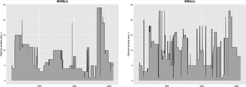
Figure 8 plots the optimal window size $n_t^{\ast }$ in the $MOM\left(n\right)$ and $SMA\left(n\right)$ rules over a rolling period of 10 years against the start of the rolling period. The first reported value for the optimal window size is for the 10-year period from January 1860 to December 1869, the second value is for the 10-year period from February 1860 to January 1870, and so forth. Our results clearly demonstrate that in any rule, there is no single optimal size of the averaging window. In contrast, the results indicate that there are substantial time-variations in the size of the optimal averaging window. Specifically, we find that for the $MOM\left(n\right)$ rule, the optimal window size varies from 1 to 24 months with a mean (median) value of 7.9 (6) months. For the $SMA\left(n\right)$ rule, the optimal size varies from 1 to 23 months with a mean (median) value of 9.8 (10) months.¹⁴ Finally, it is worth noting that qualitatively similar results can also be obtained for the LMA and EMA rules.

Figure 8. The optimal size of the averaging window in the $MOM\left(n\right)$ and $SMA\left(n\right)$ rules over a rolling period of 10 years. The first reported value for the optimal window size is for the 10-year period from January 1860 to December 1869, the second value is for the 10-year period from February 1860 to January 1870, and so forth.

7.2. Measuring the empirical trend strength

Are there trends in the S&P Composite index? If there are, what is the strength of these trends? We remind the reader that our measure of trend strength is α, which is the sum of the autoregressive coefficients of the $AR\left(p\right)$ process for returns. The most straightforward approach to measuring the empirical strength of trends is based on estimating the autoregressive coefficients using the following OLS regression model and finding the sum of the autoregressive coefficients: $X_t=a+\sum _{i=1}^p{\phi }_i{X}_{t-i}+{\epsilon }_t.$ Table 2 reports the results of the estimation of the empirical trend strength of the S&P Composite index using the sum of the autoregressive coefficients. Specifically, using the data for the total sample and the first and second halves of the sample, the table reports the estimated autoregressive coefficients and the sum of the coefficients. The number of lags p = 12 is chosen to capture the short-term momentum in the S&P Composite index. In sum, the empirical results suggest the presence of relatively weak stock market trends ($\alpha =0.26$) in the first half of the sample and the absence of stock market trends ($\alpha =0.08$) in the second half of the sample over the period from 1938 to 2017. This result is very surprising given that numerous empirical studies report that trend-following rules have also been profitable in the post-1938 period.

Table 2. Estimation of trend strength using the sum of the autoregressive coefficients.

	1858–2017		1858–1937		1938–2017
Parameter	Estimate	P-value	Estimate	P-value	Estimate	P-value
${\phi }_1$	0.078	0.086	0.143	0.018	0.003	0.952
${\phi }_2$	−0.003	0.938	−0.017	0.764	−0.008	0.799
${\phi }_3$	−0.075	0.084	−0.129	0.020	0.029	0.403
${\phi }_4$	0.032	0.291	0.050	0.241	0.032	0.378
${\phi }_5$	0.084	0.001	0.095	0.006	0.075	0.022
${\phi }_6$	−0.063	0.089	−0.086	0.113	−0.069	0.086
${\phi }_7$	0.027	0.390	0.068	0.141	−0.001	0.973
${\phi }_8$	0.056	0.116	0.115	0.008	−0.031	0.387
${\phi }_9$	0.016	0.706	0.019	0.710	−0.017	0.673
${\phi }_{10}$	0.015	0.628	0.057	0.164	−0.014	0.698
${\phi }_{11}$	0.009	0.787	−0.012	0.809	0.034	0.350
${\phi }_{12}$	−0.017	0.556	−0.044	0.279	0.044	0.151
α	0.159		0.261		0.077

Notes: ${\phi }_i$ denotes the lag i autocorrelation coefficient. α denotes trend strength. The standard errors are computed using the Newey-West heteroskedasticity and autocorrelation-consistent estimator with 12 lags. Bold text highlights the values that are statistically significant at the 5% level.

Why do trend-following strategies deliver superior performance in the absence of trends? In this section, we show that this puzzle can be resolved if the market returns follow the $AR\left(p\right)$ process, where both the order of the process p and the autoregressive coefficients ${\phi }_i$ vary over time. In this case, when the parameters of the $AR\left(p\right)$ process for returns change irregularly over time, the OLS regression model is not able to estimate trend strength.

How can we demonstrate the presence of trends and estimate trend strength with unstable parameters of the $AR\left(p\right)$ process for returns? Our theoretical results on the similarity between two trend-following indicators suggest a novel methodology to address these two issues. The idea is based on measuring the correlation coefficient between two trading indicators. If the returns follow a random walk, the correlation coefficient is given by equation (11(11) $Cor\left(I_t\right(n),J_t(m\left)\right)=\frac{{\mathit{\theta }}_{I,k}^{\mathrm{\prime }}{\mathit{\theta }}_{J,k}}{\parallel {\mathit{\theta }}_{I,n}\parallel \parallel {\mathit{\theta }}_{J,m}\parallel },$(11) ). Proposition 5 establishes that the correlation coefficient between trading indicators increases when trend strength, α, increases. The parameters of the $AR\left(p\right)$ process may change over time, but provided that $\alpha >0$, the correlation between the trading indicators must be higher than the correlation under the random walk. Consequently, the novel methodology to confirm the presence of trends is based on estimating the correlation coefficient $Cor\left(I_t\right(n),I_t(m\left)\right)$ and testing whether it is statistically significantly higher than the correlation coefficient under the random walk. The novel methodology to estimate trend strength is based on calculating the implied trend strength using the estimated correlation coefficient $Cor\left(I_t\right(n),I_t(m\left)\right)$.

From the numerical illustrations presented in Section 5, we know that when m diverges from n in any direction, the correlation between two MOM rules, $Cor\left(MOM\right(n),MOM(m\left)\right)$, decreases much faster than the correlation between two MA rules. Therefore, to demonstrate the presence of trends and estimate the empirical trend strength, it is advantageous to use trading indicators of MOM rules.

The formal description of the novel methodology to demonstrate the presence of trends is as follows. First, we estimate the empirical correlation coefficient between two MOM rules $Co{r}_{EMP}\left(MOM\right(n),MOM(m\left)\right)$. Then, we test whether the empirical correlation coefficient is statistically significantly higher than the correlation coefficient under the random walk $Co{r}_{RW}\left(MOM\right(n),MOM(m\left)\right)$. For this purpose, we formulate and conduct a test of the following null hypothesis: $\begin{array}{rl}& H_0:Co{r}_{EMP}\left(MOM\right(n),MOM(m\left)\right)\\ & \le Co{r}_{RW}\left(MOM\right(n),MOM(m\left)\right).\end{array}$ It is worth noting that under the null hypothesis, the returns follow a random walk, and the empirically estimated correlation coefficient is not greater than the true correlation under the random walk. Since under the null condition, there is no dependence in the return series, to conduct the test of the null hypothesis, we employ the randomization method. The randomization method was introduced by Fisher (1935) and provides a very general and robust approach for computing the probability of obtaining some specific value for an estimator under the null hypothesis of no dependence. We refer interested readers to Noreen (1989) and Manly (1997) for extensive discussions of the randomization tests. In summary, randomization consists of reshuffling the data to destroy any dependence and then recalculating the test statistics for each reshuffling to estimate its distribution under the null hypothesis of no dependence. The great advantage of the randomization method is that it is very simple, and no assumptions are made about the actual distribution of stock returns.

To be more specific, the estimation of the p-value of the test is conducted as follows. To learn the sampling distribution for $Co{r}_{RW}\left(MOM\right(n),MOM(m\left)\right)$, we randomize the original return series. This is repeated 1,000 times, each time obtaining a new estimate for $Co{r}_{RW}\left(MOM\right(n),MOM(m){)}^{\ast }$.¹⁵ Finally, to estimate the significance level, we count how many times the estimated value for $Co{r}_{RW}\left(MOM\right(n),MOM(m){)}^{\ast }$ after randomization falls above the value of the actual estimate for $Co{r}_{EMP}\left(MOM\right(n),MOM(m\left)\right)$. In other words, under the null hypothesis, we compute the probability of obtaining a more extreme value for the correlation coefficient than the actual estimate.

Once we establish the presence of trends, we can compute the implied trend strength. The notion of ‘implied trend strength’ is motivated by the notion of implied volatility in option prices. In our context, the implied trend strength is the sum of the autoregressive coefficients, which, when input in formula (8(8) $Cor\left(I_t\right(n),J_t(m\left)\right)=\frac{{\mathit{\theta }}_{I,n}^{\mathrm{\prime }}{\mathit{P}}_{n,m}{\mathit{\theta }}_{J,m}}{\sqrt{{\mathit{\theta }}_{I,n}^{\mathrm{\prime }}{\mathit{P}}_{n,n}{\mathit{\theta }}_{I,n}}\sqrt{{\mathit{\theta }}_{J,m}^{\mathrm{\prime }}{\mathit{P}}_{m,m}{\mathit{\theta }}_{J,m}}},$(8) ) for the correlation coefficient between the trading indicators, will return the empirically estimated value of the correlation coefficient. Specifically, when the returns follow a specific $AR\left(p\right)$ process, the correlation coefficient between two trading indicators is given by equation (8(8) $Cor\left(I_t\right(n),J_t(m\left)\right)=\frac{{\mathit{\theta }}_{I,n}^{\mathrm{\prime }}{\mathit{P}}_{n,m}{\mathit{\theta }}_{J,m}}{\sqrt{{\mathit{\theta }}_{I,n}^{\mathrm{\prime }}{\mathit{P}}_{n,n}{\mathit{\theta }}_{I,n}}\sqrt{{\mathit{\theta }}_{J,m}^{\mathrm{\prime }}{\mathit{P}}_{m,m}{\mathit{\theta }}_{J,m}}},$(8) ). The idea is to note that the correlation coefficient is the function of the return weights and the autoregressive coefficients (19) $Cor\left(I_t\right(n),I_t(m\left)\right)=f({\mathit{\theta }}_{I,n},{\mathit{\theta }}_{I,m},{\phi }_1,\dots ,{\phi }_p).$(19) For simplicity, we assume that ${\phi }_i=0$ for i>1. In this simplified case, the implied trend strength $\alpha ={\phi }_1$. It is generally not possible to invert formula (19(19) $Cor\left(I_t\right(n),I_t(m\left)\right)=f({\mathit{\theta }}_{I,n},{\mathit{\theta }}_{I,m},{\phi }_1,\dots ,{\phi }_p).$(19) ) such that the implied α is expressed as a function of $Cor\left(I_t\right(n),I_t(m\left)\right)$, ${\mathit{\theta }}_{I,n}$, and ${\mathit{\theta }}_{I,m}$. However, the implied trend strength can easily be computed using, for example, an iterative search procedure.

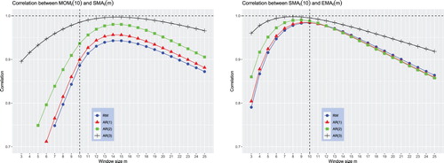
Table 3 reports the estimated correlations $Co{r}_{EMP}\left(MOM\right(n),MOM(m\left)\right)$ and the results of testing the null hypothesis for various choices of n and m using the full sample of data and the data for the first and second halves of the sample. All correlations are estimated using the robust correlation estimation method suggested by Rousseeuw and Driessen (1999). In sum, the results reported in this table argue that, regardless of the choice of the sample period and the values of n and m, the empirical correlation between the trading indicators $Co{r}_{EMP}\left(MOM\right(n),MOM(m\left)\right)$ is statistically significantly higher than the correlation under the random walk $Co{r}_{RW}\left(MOM\right(n),MOM(m\left)\right)$.

Table 3. Detection of the presence of trends and estimation of trend strength using the empirical correlation between the trading indicators of the $MOM\left(n\right)$ and $MOM\left(m\right)$ rules.

	1858–2017		1858–1937		1938–2017
Parameter	Estimate	P-value	Estimate	P-value	Estimate	P-value
Panel A: Results for n = 9 and m = 4.
$Co{r}_{RW}$	0.667		0.667		0.667
$Co{r}_{EMP}$	0.717	0.003	0.726	0.003	0.725	0.016
Implied α	0.438		0.480		0.477
Panel B: Results for n = 10 and m = 4.
$Co{r}_{RW}$	0.632		0.632		0.632
$Co{r}_{EMP}$	0.680	0.003	0.676	0.010	0.679	0.036
Implied α	0.458		0.436		0.449
Panel C: Results for n = 10 and m = 5.
$Co{r}_{RW}$	0.707		0.707		0.707
$Co{r}_{EMP}$	0.767	0.000	0.771	0.001	0.765	0.017
Implied α	0.511		0.529		0.514

Notes: $Co{r}_{RW}$ denotes the theoretical correlation between the trading indicators under the random walk. $Co{r}_{EMP}$ denotes the empirical estimate of the correlation between the trading indicators. Implied α denotes the implied trend strength. Bold text highlights the values that are statistically significant at the 5% level.

The results in table 3 on estimates of the implied trend strength based on using the estimated correlation between two trading indicators differ remarkably from the results in table 2 on the estimates of trend strength based on using the sum of the estimated autocorrelation coefficients. In particular, the results in table 2 suggest the presence of weak trends in the first half of the sample and the absence of trends in the second half of the sample. In contrast, the results in table 3 reveal the presence of substantial market trends of approximately the same strength in both halves of the sample. These trends are equivalent to the case in which the market returns follow an AR(1) process with an autoregressive coefficient of approximately 0.45-0.50. Therefore, given this result, it is not surprising that the trend-following strategies delivered superior performance in both halves of the sample.

In closing this section, we would like to note that the value of the implied alpha depends not only on the difference between $Co{r}_{EMP}$ and $Co{r}_{RW}$ but also on the order of the autoregressive process $AR\left(p\right)$. Generally, the larger the value of p is, the smaller the value of the implied alpha. Therefore, the values of the implied alphas reported in table 3 must be treated with caution. However, regardless of the choice of the autoregressive order p, the estimated implied alphas for the first and second halves of the sample are of approximately the same value. Therefore, strictly speaking, our empirical study demonstrates the presence of trends in the S&P Composite index and establishes that the empirical trend strength was about the same in both halves of the sample. However, there is some ambiguity regarding the exact measurement of the trend strength.

7.3. Predicting the future return under uncertain order of AR process

This section presents a feasible model where the MA rules are better, on average, than the MOM rule. As before, in our model, the returns follow an $AR\left(p\right)$ process. However, we assume in addition that the number of autoregressive terms p in the $AR\left(p\right)$ process is a random variable. Specifically, the number of autoregressive terms p changes randomly over time, and the trader has no ability to learn the current value of p.¹⁶ We further suppose that for any p, the values of all ${\phi }_i$ coefficients in the $AR\left(p\right)$ model are alike. That is, ${\phi }_i=\phi$ for all $i\in [1,p]$.

It is worth noting that if the trader knows the value of p, the optimal trading rule is $MOM\left(p\right)$. This is because in our model, the trading indicator of the $MOM\left(p\right)$ rule provides the highest possible correlation with the future return. The situation changes when the return process has an uncertain order of autoregression. That is, when the number of autoregressive terms in the $AR\left(p\right)$ process changes randomly.

To make our model tractable, we assume that p is uniformly distributed on $[1,20]$. The choices of the minimum and maximum values for p are motivated by the empirical study presented in Section 7.1. The value of φ in our model is chosen such that for all $p\in [1,20]$, the correlation $Cor(X_{t+1},MO{M}_t(p\left)\right)$ is constant¹⁷ and equals 0.2.¹⁸ Note that given some p, the correlation between the trading indicator of the $MOM\left(p\right)$ rule and future returns is the highest possible correlation between the trading indicator of a trend-following rule and the future return when ${\phi }_i=\phi$ for all $i\in [1,p]$. Formally, $Cor(X_{t+1},I_t(n\left)\right)\le Cor(X_{t+1},MO{M}_t(p\left)\right)=0.2$.

We further assume that the trader knows the probability distribution of p and chooses the size of the averaging window n that maximizes the average correlation over all p. This assumption is quite realistic in situations where the trader uses a very long-term historical sample to backtest a trading rule. Specifically, if the probability distribution of p is stationary over time and the historical sample is very long, then the outcome of such a backtest is the averaging window size, which is optimal on average, over all possible realizations of p. If the investor uses the trading indicator with window size n, the average correlation of this indicator with the future return is given by $\begin{array}{rl}& \overline{Cor}\left(X_{t+1}\right(p),I_t(n\left)\right)\\ & =\frac{1}{p^{max}-p^{min}+1}\sum _{p=p^{min}}^{p^{max}}Cor\left(X_{t+1}\right(p),I_t(n\left)\right),\end{array}$ where the notation $X_{t+1}\left(p\right)$ emphasizes that $X_{t+1}$ follows a particular $AR\left(p\right)$ process and $\overline{Cor}(\cdot )$ denotes the average correlation between $X_{t+1}\left(p\right)$ and $I_t\left(n\right)$. In our model, the trader solves the following problem: $n^{\ast }=\arg \underset{n}{max}\overline{Cor}\left(X_{t+1}\right(p),I_t(n\left)\right),$ where $n^{\ast }$ denotes the optimal size of the averaging window that maximizes the average correlation.

For the MOM and all MA rules, figure 9 plots the average correlation $\overline{Cor}\left(X_{t+1}\right(p),I_t(n\left)\right)$ against the window size n. For each rule, table 4 reports the maximum average correlation between the trading indicator and future return, as well as the optimal size of the averaging window $n^{\ast }$ at which the correlation attains its maximum. The results reported in figure 9 and table 4 clearly demonstrate that the MOM rule is inferior to any MA rule under uncertain market dynamics when the returns follow the $AR\left(p\right)$ process where the number of autoregressive terms changes randomly. The trader is better off by using an MA rule instead of the MOM rule.

Figure 9. The average correlation $\overline{Cor}\left(X_{t+1}\right(p),I_t(n\left)\right)$ when $X_{t+1}$ follows the $AR\left(p\right)$ process where p is uniformly distributed on $[1,20]$.

Table 4. The maximum average correlation $\overline{Cor}\left(X_{t+1}\right(p),I_t(n\left)\right)$, as well as the optimal size of the averaging window $n^{\ast }$ that maximizes the average correlation, when $X_{t+1}$ follows the $AR\left(p\right)$ process where p is uniformly distributed on $[1,20]$.

Trading rule	MOM	SMA	LMA	EMA
Maximum average correlation	0.166	0.175	0.176	0.176
n that maximizes the average correlation	10	15	21	15

Specifically, if the trader chooses the MOM rule, the trading indicator that maximizes the average correlation is MOM(10). In this case, the average correlation between the trading indicator of the $MOM\left(10\right)$ rule and future returns amounts to 0.166. However, replacing the MOM(10) rule with either the LMA(21) or EMA(15) rule increases the average correlation to 0.176. In addition, figure 9 also indicates that the trading indicator of the EMA rule virtually always provides a higher average correlation with the next period return than that of the MOM rule. Generally, in our model, the trading indicator of all MA rules provides a higher maximum average correlation with the future return than that of the MOM rule. For a small value of n, the average correlation of the MOM rule is higher than that of the SMA and LMA rules. The situation changes dramatically when n becomes large. Specifically, in this case, the average correlation of the SMA and LMA rules is substantially higher than that of the MOM rule.

Why does the trading indicator of an MA rule provide a higher average correlation with the future return and thus predict the future return better than the trading indicator of the MOM rule under uncertain market dynamics? At first glance, this result is surprising given the fact that the $AR\left(p\right)$ process (where ${\phi }_i=\phi$) seems to favor using the MOM rule. The explanation for this result is based on the properties of the correlation $Cor(X_{t+1},I_t(n\left)\right)$ established in Section 6. Specifically, the numerical illustrations presented in Section 6 persuasively demonstrate that, compared to the MOM rule, the correlation between the trading indicator of an MA rule and future returns is more robust to the change in the size of the averaging window n.

In concluding this section, we must mention the following. First, the advantage of an MA rule over the MOM rule under uncertain market dynamics increases if we assume that the values of the autoregressive terms in the $AR\left(p\right)$ process linearly decrease. Second, the numerical results on the average correlations, reported in figure 9 and table 4, are obtained under the specific choices for the correlation $Cor(X_{t+1},MO{M}_t(p\left)\right)$ and the range values for p. The average correlations between the trading indicator and the future return change when we change the correlation $Cor(X_{t+1},MO{M}_t(p\left)\right)$ and the range values for p. However, regardless of the value of the correlation coefficient¹⁹ $Cor(X_{t+1},MO{M}_t(p\left)\right)$ in situations where the difference between $p_{min}$ and $p_{max}$ is noticeable, the main message of this section remains intact: the MOM rule is inferior to any MA rule under uncertain market dynamics.

7.4. Empirical study of robustness of trading rules

The contemporary approach to selecting the best trading rule is based on the backtesting methodology. In the context of our study, backtesting consists of using a sample of historical data, simulating the returns to various $MOM\left(n\right)$ and $MA\left(n\right)$ rules, and selecting the rule with the best observed performance in the past. Specifically, by varying the window size n, the trader simulates the returns to a set of distinct MOM and MA trading rules and evaluates the historical performance of each rule. Finally, the best performing trading rule is selected. It is worth emphasizing that the best performing rule is specified not only by the weighting function for returns but also by the specific size n of the averaging window. This specific window size is usually regarded as the optimal window size. The standard assumption is that the best trading rule in a backtest will continue to deliver superior performance in the future.

The results of our empirical study conducted in Section 7.1 suggest that, regardless of the choice of a trading rule, there is no window size that is optimal at any given time. In contrast, there are substantial time-variations in the optimal size of the averaging window for each trading rule. The recognition of this fact raises several issues that can potentially undermine the results of a backtest. First, if the historical sample covers a long-term period, then the optimal window size found in a backtest must be interpreted as the window size that is optimal on average. If the historical sample covers a short-term period, then the found optimal window size is specific to this concrete historical period and not to any other period. Second, the optimal window size is subject to estimation errors. Third, we can question on general grounds the implicit assumption in a backtest that the window size that was optimal in the past will also be optimal in the future. Overall, all these issues suggest that there is absolutely no guarantee that the best trading rule in a backtest will continue to deliver superior performance in the near future.

The methodology of the empirical study in this section is based on the premise that the trader explicitly acknowledges the fact that the optimal window size in any trading rule changes randomly over time. Therefore, a backtest might be a poor guide to selecting the window size in a trading rule. Alternatively, the averaging window size in a trading rule can be chosen arbitrarily. In our study, the goal of the trader is to select the trading rule that exhibits the most robust performance with respect to the choice of the averaging window size.

Effectively, the methodology of our empirical study in this section resembles the stress testing methodology, where the goal is to determine the stability and robustness of a given system or entity. In addition, the goal of our study is to empirically confirm the validity of our theoretical predictions on the robustness of trading rules to changes in the averaging window size. Our study complements the results reported in numerous published papers that conduct back and forward tests²⁰ of various trend-following rules and provides additional valuable information on the performance robustness of these rules.

We now turn to the formal presentation of the methodology of our study. In accordance with our premise, the trader accepts the fact that the optimal window size for the near future is unknown, so the trader randomly chooses the averaging window size. Specifically, in every trading rule, the window size n is chosen in the range $[n^{min},n^{max}]$, where each value has equal probability. The goal of the trader is to find the trading rule that delivers the highest average performance over all randomly chosen window sizes. For this purpose, using a long-term historical sample of data, the trader simulates the returns to trading rule i with various window sizes, evaluates the performance of each combination, and computes the average Sharpe ratio: ${\overline{SR}}_i=\frac{1}{n^{max}-n^{min}+1}\sum _{n=n^{min}}^{n^{max}}S{R}_i\left(n\right),$ where $S{R}_i\left(n\right)$ denotes the Sharpe ratio of trading rule i with window size n.

To conduct statistical inference, we test the null hypothesis that two trading rules have equal average Sharpe ratios: $H_0:{\overline{SR}}_i={\overline{SR}}_j,$ where ${\overline{SR}}_i$ and ${\overline{SR}}_j$ are the average Sharpe ratios of trading rules i and j, respectively. To test the null hypothesis, we conduct the Wilcoxon signed-rank test instead of the paired Student's t-test because the sample size for the Sharpe ratio is small and the population cannot be assumed to be normally distributed. The Wilcoxon signed-rank test is a nonparametric test that is used to compare the locations of two populations. The method employed is a sum of ranks comparison. Therefore, the Wilcoxon test is robust to outliers in the populations.

For the sake of comparability with the results of previously published studies, in this study, n denotes the number of price (not return) observations. We assume that $n^{min}=2$, which is the lowest possible value for n, whereas $n^{max}=24$. The latter choice is motivated by the empirical study presented in Section 7.1 and our theoretical model in Section 7.3. Table 5 reports the average Sharpe ratios of the MOM and MA trading rules as well as the p-values of the test of the equality of the average Sharpe ratios of two different rules. To illustrate the robustness of our findings, we report the results for the total sample (1858–2017) as well as for the first (1858–1937) and the second (1938–2017) halves of the sample.

Table 5. Average Sharpe ratios of the MOM and MA trading rules and the p-values of the test of equality of the average Sharpe ratios of two different rules.

	Trading rule
	MOM	SMA	LMA	EMA
Panel A: 1858–2017
Average Sharpe ratio	0.438	0.487	0.485	0.459
P-value	MOM	0.021	0.021	0.256
	SMA		0.637	0.025
	LMA			0.013
Panel B: 1858–1937
Average Sharpe ratio	0.397	0.466	0.460	0.425
P-value	MOM	0.013	0.036	0.499
	SMA		0.410	0.029
	LMA			0.027
Panel B: 1938–2017
Average Sharpe ratio	0.510	0.554	0.560	0.527
P-value	MOM	0.036	0.025	0.197
	SMA		0.904	0.068
	LMA			0.001

Notes: P-values in bold text indicate a significant difference at the 5% level.

Generally, the results reported in table 5 confirm the predictions made by our theoretical models. In particular, our theoretical models predict that the forecast accuracy of the MA rules is more robust to a change in the size of the averaging window than that of the MOM rule. Therefore, under uncertain market dynamics, the MA rules possess an advantage over the MOM rule. There is, however, one notable discrepancy between the empirical results and the predictions made by our model considered in the preceding section. In particular, whereas our theoretical model implies that there should not be notable differences between the performances of the MA rules, the results of our empirical study suggest that the average performance of the EMA rule is statistically significantly below those of the SMA and LMA rules, and we cannot reject the hypothesis that it equals the average performance of the MOM rule. In agreement with the predictions of our theoretical models, the average performance of the SMA and LMA rules is higher than that of the MOM rule, and this advantage is highly statistically significant. In this study, the economic advantage of the SMA and LMA rules over the MOM rule can be roughly estimated as follows. The standard deviation of the returns to a trend-following strategy is fairly stable and amounts to approximately 11% in annual terms (Zakamulin 2017). The average Sharpe ratio of the SMA and LMA rules is approximately 10% greater than that of the MOM rule. Therefore, in our study, over the second half of our sample, 1938–2017, the SMA and LMA rules generated, on average, an annual return that is approximately 1% higher than that of the MOM rule.

Additional valuable insights about the performance robustness of the trading rules to the choice of the window size are provided in figure 10. This figure plots the Sharpe ratios of the trading rules versus the averaging window size over the total historical sample from 1858 to 2017. The curves in this figure bear clear qualitative similarities (with some quantitative differences) to the curves in figure 9 that come from our simple theoretical model. The first similarity is that as the window size n increases, the Sharpe ratio of a trading rule first increases, attains a maximum, and then decreases. The Sharpe ratio of the MOM rule attains a maximum at n = 11. For the SMA, LMA, and EMA rules, the maximum is attained at n = 12, n = 22, and n = 13, respectively. All these values are close to the values predicted by our theoretical model in the preceding section (see table 4). As mentioned above, the main dissimilarity between the predictions of our theoretical model and the empirical findings is the poor performance of the EMA rule compared to those of the SMA and LMA rules. Qualitatively, the relative empirical performance of the other rules is completely in agreement with the predictions made by our theoretical model. Specifically, when n is rather short, the MOM rule outperforms both the SMA and LMA rules. When n increases, the SMA rule outperforms the MOM and LMA rules. A further increase in n makes the LMA (MOM) rule the best (worst) performing rule.

Figure 10. The Sharpe ratios of the trading rules against the averaging window size over the total historical sample from 1858 to 2017.

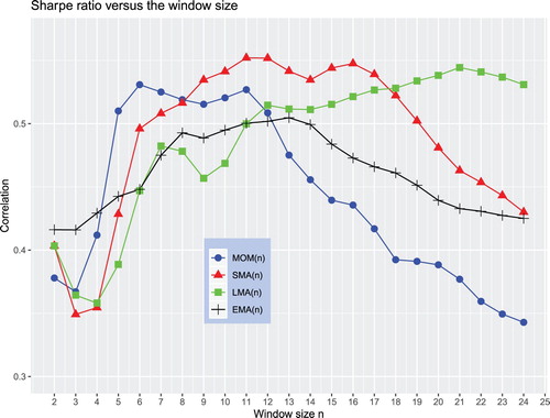
In closing this section, it is worth emphasizing that the window size that is best for the MOM rule is not necessarily best for an MA rule. Even though the performance of each rule is, to a large extent, robust to the choice of the averaging window size, the MOM rule performs well when the window size lies in the range $n\in [5,12]$. The SMA is the best performing rule for $n\in [9,17]$. The LMA rule delivers fairly stable performance for $n\in [12,30]$.

8. Conclusions

Despite the ever-growing interest in trend following and a series of publications in academic journals, there remains a dearth of theoretical results on the properties of trend-following rules. Our paper fills this gap by comparing and contrasting the two most popular trend-following rules, MOM and MA, from a theoretical perspective. Our theoretical approach is based on the return-based formulation of trend-following rules and the assumption that the returns follow an autoregressive model.

We provide a number of theoretical results on the similarity between two trend-following indicators and, using numerical illustrations, demonstrate the similarity between various rules. Our results show that the similarity between the rules is fairly high even under a random walk. The similarity between the rules increases with increasing trend strength. However, when two trading indicators belong to the same rule, the similarity between them decreases as the difference in the sizes of the averaging window in each indicator increase. We find that the similarity between two MA rules is more robust to change in the sizes of the averaging window than the similarity between two MOM rules.

We provide theoretical results on the forecasting properties of trend-following rules and on the parameters of the optimal trading indicator. We show that there must be a one-to-one correspondence between the return weights in the optimal trading indicator and the autoregressive coefficients in the return process. Despite this fact, our results suggest that by correctly choosing the size of the averaging window, the forecast accuracy of any trading indicator can be brought very close to that provided by the optimal trading indicator. We demonstrate that the forecast accuracies of trend-following rules differ mainly in their robustness to the change in the size of the averaging window and the order of the autoregressive process for returns. We find that the trading indicators of the MA rules deliver more robust forecast accuracy than the trading indicator of the MOM rule.

Finally, in this paper, we suggest and develop a well-motivated hypothesis that market returns follow an autoregressive process, the parameters of which change randomly over time. We show that our hypothesis, coupled with our analytical results on the similarity between two trading indicators and the similarity between a trading indicator and future returns, has far-reaching practical implications and is able to explain a number of empirical observations. Among other things, our hypothesis explains why traders disagree on the optimal size of the averaging window in a trading rule and the practical difficulties in establishing the presence of market trends. Our theoretical results on the similarity between two trading indicators call for a novel methodology to demonstrate the presence of trends and estimate the strength of these trends under uncertain market dynamics. Based on our hypothesis, we construct a theoretical model that implies that on average, the trading indicators of the MA rules tend to forecast the future return better than the trading indicator of the MOM rule. The validity of our theoretical predictions on the relative performance robustness of trading rules under uncertain market dynamics is empirically confirmed by a novel empirical study.

Overall, our paper presents an in-depth analysis of the commonalities and differences between the MOM and MA rules. We broaden the appeal and practical importance of our theoretical results by offering a number of illustrations and real-world examples. The results reported in this paper can help traders better understand the properties of the most popular trend-following rules.

Disclosure statement

No potential conflict of interest was reported by the authors.

ORCID

Valeriy Zakamulin http://orcid.org/0000-0002-8619-7283

Notes

1 See, among others, Brock et al. (1992), Faber (2007), Gwilym et al. (2010), Kilgallen (2012), Moskowitz et al. (2012), Clare et al. (2013), Neely et al. (2014), Marshall et al. (2017), and Faber (2017).

2 The technical indicator of a trading rule is a mathematical function that formalizes how past prices are used to forecast the future direction of the price trend.

3 Gartley (1935) is regarded as the pioneering book where the author laid the foundations for technical trading based on moving averages of prices.

4 In this case, the EMA can be computed using the following recursive form that greatly facilitates and accelerates the computation: $EM{A}_t\left(n\right)=(1-\lambda )P_t+\lambda EM{A}_{t-1}\left(n\right)$.

5 http://schwert.ssb.rochester.edu/data.htm

6 http://www.hec.unil.ch/agoyal/

7 http://research.stlouisfed.org/fred2/series/M13002US35620M156NNBR

8 Note that the trading indicator in the EMA rule is computed using an infinite size of the averaging window. Consequently, for the EMA rule the $n\times m$ matrix $\mathit{P}$ is, in fact, the matrix of dimensions $\mathrm{\infty }\times \mathrm{\infty }$. In this case, the exact numerical computation of the correlation coefficient is not feasible. To address this problem, in our numerical illustrations, the computation of a correlation coefficient is conducted using the $k\times k$ matrix $\mathit{P}$, where the value of k is chosen such that ${\theta }_k/{\theta }_0=0.01$. Recall that the ${\theta }_i$ coefficients in the EMA rule exponentially decrease as i increases. With our choice of k, the value of ${\theta }_k$ amounts to 1% of the value of ${\theta }_0$.

9 Note that both $SM{A}_t\left(1\right)$ and $LM{A}_t\left(1\right)$ are equivalent to $MO{M}_t\left(1\right)$, whereas the $EM{A}_t\left(1\right)$ indicator is not defined.

10 The default spread is the difference between the yields on BAA- and AAA-rated corporate bonds

11 The term premium is the difference between the yields on long-term bonds and the short-term rate.

12 That is, the returns in excess of the risk-free rate of return. Note further that in our empirical study, the trading indicator is computed using capital gain returns. This is because traders traditionally compute the trading indicator using prices not adjusted for dividends.

13 To conduct a backtest, we need both bull and bear markets in a selected historical period in order a trend-following rule generates both buy and sell signals.

14 These results advocate that the most popular SMA(10) rule is not the rule that is optimal at any given time. Rather, it is the rule that is optimal on average, over all possible realizations of the stock market dynamics.

15 The asterisk is used to indicate that each of these estimates is calculated on a randomized sample.

16 When the number of autoregressive terms is deterministic, the number p can be estimated using past data on returns. In our model, since p changes randomly, past data cannot reveal the current number of autoregressive terms in the model for returns.

17 Our method of choosing the value of $\phi =\phi \left(p\right)$ guarantees that for all p, the $AR\left(p\right)$ process satisfies the stationarity conditions.

18 This choice is partially motivated by our econometric study on the empirical trend strength presented in Section 7.2. Specifically, if $\alpha ={\phi }_1=0.5$, then the correlation between the future return and the trading indicator of the $MOM\left(10\right)$ rule approximately equals 0.2. The selected value of n = 10 lies in the middle of the range of possible values of p.

19 We only need to require $Cor(X_{t+1},MO{M}_t(p\left)\right)>0$.

20 Back (forward) tests are also known as in-sample (out-of-sample) tests.

Appendices

Appendix 1. Proof of Proposition 1

Each $AR\left(p\right)$ process can be represented as an infinite order Moving Average process $MA\left(\mathrm{\infty }\right)$ $X_t=\sum _{i=0}^{\mathrm{\infty }}{\psi }_i{\epsilon }_{t-i},$ where $\{{\psi }_0,{\psi }_1,{\psi }_2,\dots \}$ are parameters or MA coefficients. Hence, the autocorrelation coefficients of the $AR\left(p\right)$ process can alternatively be computed as (A1) ${\rho }_k=\sum _{i=0}^{\mathrm{\infty }}{\psi }_i{\psi }_{i+k}.$(A1) That is, each ${\rho }_k$ is an infinite sum of the products of two MA coefficients. It is known (see, for example, Box et al. 2016, page 55) that the MA coefficients of the $AR\left(p\right)$ process satisfy the following difference equation (A2) ${\psi }_j={\phi }_1{\psi }_{j-1}+{\phi }_2{\psi }_{j-2}+\cdots {\phi }_p{\psi }_{j-p}j>0$(A2) with ${\psi }_0=1$ and ${\psi }_i=0$ for j<0. From this difference equation, the coefficients ${\psi }_i$ can easily be computed recursively in terms of ${\phi }_i$. In particular, (A3) $\begin{array}{rl}{\psi }_1& ={\phi }_1,\\ {\psi }_2& ={\phi }_1{\psi }_1+{\phi }_2,\\ {\psi }_3& ={\phi }_1{\psi }_2+{\phi }_2{\psi }_1+{\phi }_3,\end{array}$(A3) and so on. From the recursive computation it becomes apparent that, when all coefficients $\{{\phi }_1,{\phi }_2,\dots ,{\phi }_p\}$ of the $AR\left(p\right)$ process are positive, then all ${\psi }_i$ coefficients of the infinite MA process are positive and, consequently, all autocorrelation coefficients ${\rho }_k$ are also positive.

Appendix 2. Proof of Proposition 2

We remind the reader that increasing the numerical value of some ${\phi }_i$ or increasing the order p increases the persistence of the $AR\left(p\right)$ process. First, consider what happens with the autocorrelation coefficients ${\rho }_k$ when we increase the value of some ${\phi }_i$. The recursive computation of the ψ coefficients, given by (A3(A3) $\begin{array}{rl}{\psi }_1& ={\phi }_1,\\ {\psi }_2& ={\phi }_1{\psi }_1+{\phi }_2,\\ {\psi }_3& ={\phi }_1{\psi }_2+{\phi }_2{\psi }_1+{\phi }_3,\end{array}$(A3) ), suggests that increasing the value of ${\phi }_i$ increases the values of all ${\psi }_j$ coefficients for $j\ge i$. Since the autocorrelation coefficients are computed according to equation (A1(A1) ${\rho }_k=\sum _{i=0}^{\mathrm{\infty }}{\psi }_i{\psi }_{i+k}.$(A1) ), increasing the value of ${\phi }_i$ increases the values of all ${\rho }_k$. Second, consider the case where we increase the order of the AR process from p to p + 1. That is, in this case we add a new autoregressive term ${\phi }_{p+1}$ to the existing $AR\left(p\right)$ process. This case is equivalent to the first case where in the original $AR(p+1)$ process the value of ${\phi }_{p+1}$ increases from zero to some positive number. Consequently, under the conditions of this proposition, increasing the persistence of the $AR\left(p\right)$ process increases the values of all autocorrelation coefficients ${\rho }_k$.

Appendix 3. Proof of Proposition 3

By definition, (A4) $Cor\left(I_t\right(n),J_t(m\left)\right)=\frac{\mathrm{C}\mathrm{o}\mathrm{v}\left(I_t\right(n),J_t(m\left)\right)}{{\sigma }_I{\sigma }_J},$(A4) where $\mathrm{C}\mathrm{o}\mathrm{v}\left(I_t\right(n),J_t(m\left)\right)$ is the covariance between indicators $I_t\left(n\right)$ and $J_t\left(m\right)$ and ${\sigma }_I$ and ${\sigma }_J$ are the standard deviations of $I_t\left(n\right)$ and $J_t\left(m\right)$ respectively.

Since by assumption $X_t$ is a zero mean process, the variance of indicator $I_t\left(n\right)$ is given by ${\sigma }_I^2=E\left[I_t\right(n\left)I_t\right(n\left)\right]=E\left[\right({\theta }_{I,0}{X}_t+{\theta }_{I,1}{X}_{t-1}+\cdots +{\theta }_{I,n-1}{X}_{t-n+1}{)}^2],$ where $E[\cdot ]$ is the expectation operator. Denote by ${\sigma }_x^2$ the variance of $X_{t-i}$. Taking into account that $E\left[X_{t-i}{X}_{t-j}\right]=\mathrm{C}\mathrm{o}\mathrm{v}\left(X_{t-i}{X}_{t-j}\right)={\rho }_{|i-j|}{\sigma }_x^2$, where ${\rho }_{|i-j|}$ denotes the correlation between $X_{t-i}$ and $X_{t-j}$, the variance of indicator $I_t\left(n\right)$ is computed as ${\sigma }_I^2=\sum _{i=0}^{n-1}\sum _{j=0}^{n-1}{\theta }_{I,i}{\theta }_{I,j}\mathrm{C}\mathrm{o}\mathrm{v}\left(X_{t-i}{X}_{t-j}\right)=\sum _{i=0}^{n-1}\sum _{j=0}^{n-1}{\theta }_{I,i}{\theta }_{I,j}{\rho }_{|i-j|}{\sigma }_x^2.$ In matrix notation, the variance of indicator $I_t\left(n\right)$ is given by (A5) ${\sigma }_I^2={\mathit{\theta }}_{I,n}^{\mathrm{\prime }}{\mathit{P}}_{n,n}{\mathit{\theta }}_{I,n}{\sigma }_x^2,$(A5) where matrix ${\mathit{P}}_{n,n}$ is given by (9(9) ${\mathit{P}}_{n,m}=\left[\begin{array}{ccccc}1& {\rho }_1& {\rho }_2& \dots & {\rho }_{m-1}\\ {\rho }_1& 1& {\rho }_1& \dots & {\rho }_{m-2}\\ {\rho }_2& {\rho }_1& 1& \dots & {\rho }_{m-3}\\ ⋮& ⋮& ⋮& \ddots & ⋮\\ {\rho }_{n-1}& {\rho }_{n-2}& {\rho }_{n-3}& \dots & {\rho }_{|m-n|}\end{array}\right],$(9) ). Similarly, the variance of indicator $J_t\left(m\right)$ is given by (A6) ${\sigma }_J^2={\mathit{\theta }}_{J,m}^{\mathrm{\prime }}{\mathit{P}}_{m,m}{\mathit{\theta }}_{J,m}{\sigma }_x^2.$(A6) By similar reasoning, the covariance between indicators $I_t\left(n\right)$ and $J_t\left(m\right)$ $\begin{array}{rl}\mathrm{C}\mathrm{o}\mathrm{v}\left(I_t\right(n),J_t(m\left)\right)& =E\left[I_t\right(n\left)J_t\right(m\left)\right]\\ & =E\left[\right({\theta }_{I,0}{X}_t+\cdots +{\theta }_{I,n-1}{X}_{t-n+1}\left)\right({\theta }_{J,0}{X}_t+\cdots \\ & +{\theta }_{J,m-1}{X}_{t-m+1}\left)\right].\end{array}$ This covariance is computed as (A7) $\begin{array}{rl}\mathrm{C}\mathrm{o}\mathrm{v}\left(I_t\right(n),J_t(m\left)\right)& =\sum _{i=0}^{n-1}\sum _{j=0}^{m-1}{\theta }_{I,i}{\theta }_{J,j}\mathrm{C}\mathrm{o}\mathrm{v}\left(X_{t-i}{X}_{t-j}\right)\\ & =\sum _{i=0}^{n-1}\sum _{j=0}^{m-1}{\theta }_{I,i}{\theta }_{J,j}{\rho }_{|i-j|}{\sigma }_x^2.\end{array}$(A7) The covariance can be expressed in matrix notation as (A8) $\mathrm{C}\mathrm{o}\mathrm{v}\left(I_t\right(n),J_t(m\left)\right)={\mathit{\theta }}_{I,n}^{\mathrm{\prime }}{\mathit{P}}_{n,m}{\mathit{\theta }}_{J,m}{\sigma }_x^2.$(A8) Inserting the expressions for $\mathrm{C}\mathrm{o}\mathrm{v}\left(I_t\right(n),J_t(m\left)\right)$, ${\sigma }_I$, and ${\sigma }_J$ into equation (A4(A4) $Cor\left(I_t\right(n),J_t(m\left)\right)=\frac{\mathrm{C}\mathrm{o}\mathrm{v}\left(I_t\right(n),J_t(m\left)\right)}{{\sigma }_I{\sigma }_J},$(A4) ) completes the proof.

Appendix 4. Proof of Proposition 4

The formula for the correlation coefficient $Cor\left(I_t\right(n),J_t(m\left)\right)$ is given by equation (A4(A4) $Cor\left(I_t\right(n),J_t(m\left)\right)=\frac{\mathrm{C}\mathrm{o}\mathrm{v}\left(I_t\right(n),J_t(m\left)\right)}{{\sigma }_I{\sigma }_J},$(A4) ). Since the standard deviations are positive, the sign of the correlation coefficient depends on the sign of the covariance $\mathrm{C}\mathrm{o}\mathrm{v}\left(I_t\right(n),J_t(m\left)\right)$.

The expression for the computation of the covariance is given by equation (A7(A7) $\begin{array}{rl}\mathrm{C}\mathrm{o}\mathrm{v}\left(I_t\right(n),J_t(m\left)\right)& =\sum _{i=0}^{n-1}\sum _{j=0}^{m-1}{\theta }_{I,i}{\theta }_{J,j}\mathrm{C}\mathrm{o}\mathrm{v}\left(X_{t-i}{X}_{t-j}\right)\\ & =\sum _{i=0}^{n-1}\sum _{j=0}^{m-1}{\theta }_{I,i}{\theta }_{J,j}{\rho }_{|i-j|}{\sigma }_x^2.\end{array}$(A7) ). In particular, the covariance is a double sum of the product of ${\theta }_{I,i}$, ${\theta }_{J,j}$, ${\rho }_{|i-j|}$ and ${\sigma }_x^2$. In all trend following rules considered in our paper, the return weights are strictly positive. That is, ${\theta }_{I,i}>0$ and ${\theta }_{J,j}>0$ for all i and j. The variance ${\sigma }_x^2$ is also positive. The contemporaneous correlation ${\rho }_0=1$. Remains to investigate the sign of the autocorrelation coefficients ${\rho }_k$ for k>0.

According to Proposition 1, all autocorrelation coefficients ${\rho }_k$ are positive when all coefficients $\{{\phi }_1,{\phi }_2,\dots ,{\phi }_p\}$ of the $AR\left(p\right)$ process are positive. When some or all ${\phi }_i$ coefficients are zero, then all autocorrelation coefficients ${\rho }_k$ are non-negative. This result follows from the recursive equation (A2(A2) ${\psi }_j={\phi }_1{\psi }_{j-1}+{\phi }_2{\psi }_{j-2}+\cdots {\phi }_p{\psi }_{j-p}j>0$(A2) ) for the computation of the coefficients of the infinite MA process that are used to compute the autocorrelation coefficients via equation (A1(A1) ${\rho }_k=\sum _{i=0}^{\mathrm{\infty }}{\psi }_i{\psi }_{i+k}.$(A1) ). Therefore, we can conclude that the correlation coefficient $Cor\left(I_t\right(n),J_t(m\left)\right)>0$.

Appendix 5. Proof of Proposition 5

First of all, we equate the number of elements in vectors ${\mathit{\theta }}_{I,n}$ and ${\mathit{\theta }}_{J,m}$. We choose $k=max(n,m)$. If n<m, vector ${\mathit{\theta }}_{I,n}$ is augmented by m−n zero elements. Similarly, if n>m, vector ${\mathit{\theta }}_{J,m}$ is augmented by n−m zero elements. This augmentation does not change the value of the correlation but makes vectors ${\mathit{\theta }}_{I,k}$ and ${\mathit{\theta }}_{I,k}$ be of the same length $k\times 1$. Similarly, all matrices $\mathit{P}$ become $k\times k$ square matrices. As a result, in the simplified notation the expression for the correlation coefficients becomes $Cor\left(I_t\right(n),J_t(m\left)\right)=\frac{{\mathit{\theta }}_I^{\mathrm{\prime }}\mathit{P}{\mathit{\theta }}_J}{\sqrt{{\mathit{\theta }}_I^{\mathrm{\prime }}\mathit{P}{\mathit{\theta }}_I}\sqrt{{\mathit{\theta }}_J^{\mathrm{\prime }}\mathit{P}{\mathit{\theta }}_J}}=\frac{{\sigma }_{IJ}}{{\sigma }_I{\sigma }_J}.$ Proposition 2 says that increasing the persistence of the $AR\left(p\right)$ process increases the values of all autocorrelation coefficients. Consequently, increasing the persistence of the $AR\left(p\right)$ process increases all elements of matrix $\mathit{P}$. Therefore, our proof is based on the investigation of the sign of the derivative $\frac{\mathrm{\partial }Cor\left(I_t\right(n),J_t(m\left)\right)}{\mathrm{\partial }\mathit{P}}.$ A result from matrix calculus will prove helpful. Specifically, given $n\times 1$ vector $\mathit{x}$ and $n\times n$ matrix $\mathit{A}$ (A9) $\frac{\mathrm{\partial }{\mathit{x}}^{\mathbf{\prime }}\mathit{A}\mathit{x}}{\mathrm{\partial }\mathit{A}}=\mathit{x}{\mathit{x}}^{\mathbf{\prime }}.$(A9) The following partial derivatives are obtained using the result above $\frac{\mathrm{\partial }{\sigma }_I}{\mathrm{\partial }\mathit{P}}=\frac{1}{2{\sigma }_I}{\mathit{\theta }}_I{\mathit{\theta }}_I^{\mathrm{\prime }},\frac{\mathrm{\partial }{\sigma }_J}{\mathrm{\partial }\mathit{P}}=\frac{1}{2{\sigma }_J}{\mathit{\theta }}_J{\mathit{\theta }}_J^{\mathrm{\prime }},\frac{\mathrm{\partial }{\sigma }_{IJ}}{\mathrm{\partial }\mathit{P}}={\mathit{\theta }}_I{\mathit{\theta }}_J^{\mathrm{\prime }}.$ Differentiating the expression for the correlation using the quotient rule yields $\frac{\mathrm{\partial }Cor\left(I_t\right(n),J_t(m\left)\right)}{\mathrm{\partial }\mathit{P}}=\frac{2{\sigma }_I^2{\sigma }_J^2{\mathit{\theta }}_I{\mathit{\theta }}_J^{\mathrm{\prime }}-{\sigma }_{IJ}({\sigma }_J^2{\mathit{\theta }}_I{\mathit{\theta }}_I^{\mathrm{\prime }}+{\sigma }_I^2{\mathit{\theta }}_J{\mathit{\theta }}_J^{\mathrm{\prime }})}{2{\sigma }_I^3{\sigma }_J^3}.$ The derivative is positive if $2{\sigma }_I^2{\sigma }_J^2{\mathit{\theta }}_I{\mathit{\theta }}_J^{\mathrm{\prime }}>{\sigma }_{IJ}{\sigma }_J^2{\mathit{\theta }}_I{\mathit{\theta }}_I^{\mathrm{\prime }}+{\sigma }_{IJ}{\sigma }_I^2{\mathit{\theta }}_J{\mathit{\theta }}_J^{\mathrm{\prime }}.$ Pre-multiplying both sides of the inequality by ${\mathit{\theta }}_J^{\mathrm{\prime }}\mathit{P}$ and taking into account that ${\mathit{\theta }}_J^{\mathrm{\prime }}{\mathit{P}\mathit{\theta }}_I={\sigma }_{IJ}$ and ${\mathit{\theta }}_J^{\mathrm{\prime }}{\mathit{P}\mathit{\theta }}_J={\sigma }_J^2$, yields (after simplification) ${\sigma }_I^2{\mathit{\theta }}_J^{\mathrm{\prime }}>{\sigma }_{IJ}{\mathit{\theta }}_I^{\mathrm{\prime }}.$ Post-multiplying both sides of the inequality by ${\mathit{P}\mathit{\theta }}_J$ yields (after re-arrangement of the terms) $Cor\left(I_t\right(n),J_t(m){)}^2<1.$ The last inequality is true since under the conditions of this proposition $Cor\left(I_t\right(n),J_t(m\left)\right)<1$. Thus, $Cor\left(I_t\right(n),J_t(m\left)\right)$ increases with increasing persistence of the $AR\left(p\right)$ process for returns.

Appendix 6. Proof of Proposition 6

The correlation between the trading indicator $I_t\left(n\right)$ and the next period return $X_{t+1}$ is given by (A10) $Cor(X_{t+1},I_t(n\left)\right)=\frac{\mathrm{C}\mathrm{o}\mathrm{v}(X_{t+1},I_t(n\left)\right)}{{\sigma }_x{\sigma }_I},$(A10) where $\mathrm{C}\mathrm{o}\mathrm{v}(X_{t+1},I_t(n\left)\right)$ is the covariance between the trading indicator and the next period return and ${\sigma }_x$ and ${\sigma }_I$ are the standard deviations of $X_t$ and $I_t\left(n\right)$ respectively.

The variance of the trading indicator is given by equation (A5(A5) ${\sigma }_I^2={\mathit{\theta }}_{I,n}^{\mathrm{\prime }}{\mathit{P}}_{n,n}{\mathit{\theta }}_{I,n}{\sigma }_x^2,$(A5) ). The covariance between the indicator and the next period return is given by $\begin{array}{rl}& \mathrm{C}\mathrm{o}\mathrm{v}(X_{t+1},I_t(n\left)\right)\\ & =E\left[\right({\phi }_1{X}_t+{\phi }_2{X}_{t-1}+\cdots +{\phi }_p{X}_{t-p+1}+{\epsilon }_{t+1}\left)\right({\theta }_0{X}_t\\ & +{\theta }_1{X}_{t-1}+\cdots +{\theta }_{n-1}{X}_{t-n+1}\left)\right].\end{array}$ This covariance is computed as (A11) $\begin{array}{rl}\mathrm{C}\mathrm{o}\mathrm{v}(X_{t+1},I_t(n\left)\right)& =\sum _{i=0}^{p-1}\sum _{j=0}^{n-1}{\phi }_{i+1}{\theta }_j\mathrm{C}\mathrm{o}\mathrm{v}\left(X_{t-i}{X}_{t-j}\right)\\ & =\sum _{i=0}^{p-1}\sum _{j=0}^{n-1}{\phi }_{i+1}{\theta }_j{\rho }_{|i-j|}{\sigma }_x^2.\end{array}$(A11) The covariance can be expressed in matrix notation as (A12) $\mathrm{C}\mathrm{o}\mathrm{v}(X_{t+1},I_t(n\left)\right)={\mathit{\theta }}_n^{\mathrm{\prime }}{\mathit{P}}_{n,p}{\mathit{\phi }}_p{\sigma }_x^2,$(A12) where ${\mathit{\phi }}_p^{\mathrm{\prime }}=[{\phi }_1,{\phi }_2,\dots ,{\phi }_p]$ is the vector of autoregressive coefficients of $X_t$, ${\mathit{\theta }}_n$ is the vector that contains the elements of the weighting function of $I_t\left(n\right)$, and matrix ${\mathit{P}}_{n,p}$ is the matrix given by (9(9) ${\mathit{P}}_{n,m}=\left[\begin{array}{ccccc}1& {\rho }_1& {\rho }_2& \dots & {\rho }_{m-1}\\ {\rho }_1& 1& {\rho }_1& \dots & {\rho }_{m-2}\\ {\rho }_2& {\rho }_1& 1& \dots & {\rho }_{m-3}\\ ⋮& ⋮& ⋮& \ddots & ⋮\\ {\rho }_{n-1}& {\rho }_{n-2}& {\rho }_{n-3}& \dots & {\rho }_{|m-n|}\end{array}\right],$(9) ).

Inserting the expressions for $\mathrm{C}\mathrm{o}\mathrm{v}(X_{t+1},I_t(n\left)\right)$ and ${\sigma }_I$ into equation (A10(A10) $Cor(X_{t+1},I_t(n\left)\right)=\frac{\mathrm{C}\mathrm{o}\mathrm{v}(X_{t+1},I_t(n\left)\right)}{{\sigma }_x{\sigma }_I},$(A10) ) completes the proof.

Appendix 7. Proof of Proposition 7

The proof follows along the lines of the proof of Proposition 5. After equating the number of elements in vectors $\mathit{\theta }$ and $\mathit{\phi }$, we investigate the sign of the following derivative $\frac{\mathrm{\partial }Cor(X_{t+1},I_t(n\left)\right)}{\mathrm{\partial }\mathit{P}}=\frac{\mathrm{\partial }\frac{{\mathit{\theta }}^{\mathrm{\prime }}\mathit{P}\mathit{\phi }}{\sqrt{{\mathit{\theta }}^{\mathrm{\prime }}\mathit{P}\mathit{\theta }}}}{\mathrm{\partial }\mathit{P}}.$ Differentiating the expression for the correlation using the quotient rule yields $\frac{\mathrm{\partial }Cor\left(I_t\right(n),J_t(m\left)\right)}{\mathrm{\partial }\mathit{P}}=\frac{2{\sigma }_I^2\mathit{\theta }{\mathit{\phi }}^{\mathbf{\prime }}-\mathbf{\left(}{\mathit{\theta }}^{\mathbf{\prime }}\mathit{P}\mathit{\phi }\mathbf{\right)}\mathit{\theta }{\mathit{\theta }}^{\mathbf{\prime }}}{2{\sigma }_I^3}.$ The derivative is positive if $2{\sigma }_I^2\mathit{\theta }{\mathit{\phi }}^{\mathbf{\prime }}>\mathbf{\left(}{\mathit{\theta }}^{\mathbf{\prime }}\mathit{P}\mathit{\phi }\mathbf{\right)}\mathit{\theta }{\mathit{\theta }}^{\mathbf{\prime }}.$ Post-multiplying both sides of the inequality by $\mathit{P}\mathit{\theta }$ and taking into account that ${\mathit{\theta }}^{\mathbf{\prime }}\mathit{P}\mathit{\theta }={\sigma }_I^2$ and ${\mathit{\phi }}^{\mathbf{\prime }}\mathit{P}\mathit{\theta }={\mathit{\theta }}^{\mathbf{\prime }}\mathit{P}\mathit{\phi }$, we get $2{\sigma }_I^2\mathit{\theta }>{\sigma }_I^2\mathit{\theta }.$ The last inequality is true since $2{\sigma }_I^2>{\sigma }_I^2$. Thus, $Cor(X_{t+1},I_t(n\left)\right)$ increases with increasing persistence of the $AR\left(p\right)$ process for returns.

Appendix 8. Proof of Proposition 8

Our goal is to find the solution of the following maximization problem $\underset{{\mathit{\theta }}_n}{max}Cor(X_{t+1},I_t(n\left)\right)=\frac{{\mathit{\theta }}_n^{\mathrm{\prime }}{\mathit{P}}_{n,p}{\mathit{\phi }}_p}{\sqrt{{\mathit{\theta }}_n^{\mathrm{\prime }}{\mathit{P}}_{n,n}{\mathit{\theta }}_n}}.$ First of all, we equate the number of elements in vectors ${\mathit{\theta }}_n$ and ${\mathit{\phi }}_p$. We choose $k=max(n,p)$. If n<p, vector ${\mathit{\theta }}_n$ is augmented by p−n zero elements. Similarly, if n>p, vector ${\mathit{\phi }}_p$ is augmented by n−p zero elements. This augmentation does not change the value of the correlation but makes vectors ${\mathit{\theta }}_k$ and ${\mathit{\phi }}_k$ be of the same length. To simplify notation, in the expressions below we omit the subscripts in the vectors and matrices.

The first-order condition of optimality of $\mathit{\theta }$ is given by $\frac{\mathrm{\partial }Cor(X_{t+1},I_t(n\left)\right)}{\mathrm{\partial }\mathit{\theta }}=0.$ The expression for the correlation coefficient represents a ratio of two functions. Therefore, we apply the quotient rule of differentiation $(F/G{)}^{\mathrm{\prime }}=(F^{\mathrm{\prime }}G-G^{\mathrm{\prime }}F)/G^2$. $F^{\mathrm{\prime }}=\frac{\mathrm{\partial }{\mathit{\theta }}^{\mathrm{\prime }}\mathit{P}\mathit{\phi }}{\mathrm{\partial }\mathit{\theta }}=\mathit{P}\mathit{\phi },G^{\mathrm{\prime }}=\frac{\mathrm{\partial }\sqrt{{\mathit{\theta }}^{\mathrm{\prime }}\mathit{P}\mathit{\theta }}}{\mathrm{\partial }\mathit{\theta }}=\frac{\mathit{P}\mathit{\theta }}{\sqrt{{\mathit{\theta }}^{\mathrm{\prime }}\mathit{P}\mathit{\theta }}}.$ As a result, the first-order condition of optimality is given by $\frac{\mathit{P}\mathit{\phi }\left({\mathit{\theta }}^{\mathrm{\prime }}\mathit{P}\mathit{\theta }\right)-\mathit{P}\mathit{\theta }\left({\mathit{\theta }}^{\mathrm{\prime }}\mathit{P}\mathit{\phi }\right)}{{\mathit{\theta }}^{\mathrm{\prime }}\mathit{P}\mathit{\theta }\sqrt{{\mathit{\theta }}^{\mathrm{\prime }}\mathit{P}\mathit{\theta }}}=0.$ The first order condition reduces to (A13) $\mathit{P}\mathit{\phi }\left({\mathit{\theta }}^{\mathrm{\prime }}\mathit{P}\mathit{\theta }\right)=\mathit{P}\mathit{\theta }\left({\mathit{\theta }}^{\mathrm{\prime }}\mathit{P}\mathit{\phi }\right).$(A13) It is easy to note that if $\mathit{\theta }=\mathit{\phi }$, then both the vector equation $\mathit{P}\mathit{\phi }=\mathit{P}\mathit{\theta }$ and the scalar equation ${\mathit{\theta }}^{\mathrm{\prime }}\mathit{P}\mathit{\theta }={\mathit{\theta }}^{\mathrm{\prime }}\mathit{P}\mathit{\phi }$ are satisfied. Hence, when $\mathit{\theta }=\mathit{\phi }$, condition (A13(A13) $\mathit{P}\mathit{\phi }\left({\mathit{\theta }}^{\mathrm{\prime }}\mathit{P}\mathit{\theta }\right)=\mathit{P}\mathit{\theta }\left({\mathit{\theta }}^{\mathrm{\prime }}\mathit{P}\mathit{\phi }\right).$(A13) ) is satisfied. Additionally, condition (A13(A13) $\mathit{P}\mathit{\phi }\left({\mathit{\theta }}^{\mathrm{\prime }}\mathit{P}\mathit{\theta }\right)=\mathit{P}\mathit{\theta }\left({\mathit{\theta }}^{\mathrm{\prime }}\mathit{P}\mathit{\phi }\right).$(A13) ) is satisfied when $\mathit{\theta }=c\times \mathit{\phi }$ where c is any positive real number.

References

- Acar, E., Expected returns of directional forecasters. In Advanced Trading Rules, edited by E. Acar and S. Satchell, pp. 51–76, 1998 (Butterworth-Heinemann: Oxford).
- Andrews, D.W.K. and Chen, H.Y., Approximately median-unbiased estimation of autoregressive models. J. Bus. Econ. Stat., 1994, 12, 187–204.
- Ayed, A.B.H., Loeper, G. and Abergel, F., Forecasting trends with asset prices. Quant. Finance, 2017, 17, 369–382. doi: 10.1080/14697688.2016.1206959
- Beekhuizen, P. and Hallerbach, W.G., Uncovering trend rules. J. Altern. Invest., 2017, 20, 28–38. doi: 10.3905/jai.2017.20.2.028
- Box, G.E.P., Jenkins, G.M., Reinsel, G.C. and Ljung, G.M., Time Series Analysis: Forecasting and Control, Vol. 5, 2016 (John Wiley & Sons Inc: New Jersey).
- Brock, W., Lakonishok, J. and LeBaron, B., Simple technical trading rules and the stochastic properties of stock returns. J. Financ., 1992, 47, 1731–1764. doi: 10.1111/j.1540-6261.1992.tb04681.x
- Campbell, J.Y., Stock returns and the term structure. J. Financ. Econ., 1987, 118, 373–399. doi: 10.1016/0304-405X(87)90045-6
- Campbell, J.Y. and Shiller, R.J., The dividend-price ratio and expectations of future dividends and discount factors. Rev. Financ. Stud., 1988, 1, 195–227. doi: 10.1093/rfs/1.3.195
- Chen, B. and Hong, Y., Testing for smooth structural changes in time series models via nonparametric regression. Econometrica, 2012, 80, 1157–1183. doi: 10.3982/ECTA7990
- Clare, A., Seaton, J., Smith, P.N. and Thomas, S., Breaking into the blackbox: Trend following, stop losses and the frequency of trading - the case of the S&P500. J. Asset Manag., 2013, 14, 182–194. doi: 10.1057/jam.2013.11
- Dangl, T. and Halling, M., Predictive regressions with time-varying coefficients. J. Financ. Econ., 2012, 106, 157–181. doi: 10.1016/j.jfineco.2012.04.003
- Faber, M., A quantitative approach to tactical asset allocation. J. Wealth Manag., 2007, 9, 69–79. doi: 10.3905/jwm.2007.674809
- Faber, M., A quantitative approach to tactical asset allocation revisited 10 years later. J. Portfolio Manag., 2017, 44, 156–167. doi: 10.3905/jpm.2018.44.2.156
- Fama, E.F., Stock returns, real activity, inflation, and money. Am. Econ. Rev., 1981, 71, 545–565.
- Fama, E.F., Stock returns, expected returns, and real activity. J. Financ., 1990, 45, 1089–1108. doi: 10.1111/j.1540-6261.1990.tb02428.x
- Fama, E.F. and French, K.R., Business conditions and expected returns on stocks and bonds. J. Financ. Econ., 1989, 25, 23–49. doi: 10.1016/0304-405X(89)90095-0
- Fisher, R.A., The Design of Experiments, 1935 (Oliver and Boyd: Edinburgh).
- Gartley, H.M., Profits in the Stock Market, 1935 (Lambert Gann Pub: Pomeroy, WA).
- Glabadanidis, P., Timing the market with a combination of moving averages. Int. Rev. Financ., 2017, 17, 353–394. doi: 10.1111/irfi.12107
- Gonzalez, L., Powell, J.G., Shi, J. and Wilson, A., Two centuries of bull and bear market cycles. Int. Rev. Econ. Financ., 2005, 14, 469–486. doi: 10.1016/j.iref.2004.02.003
- Gwilym, O., Clare, A., Seaton, J. and Thomas, S., Price and momentum as robust tactical approaches to global equity investing. J. Invest., 2010, 19, 80–91. doi: 10.3905/joi.2010.19.3.080
- Han, Y., Zhou, G. and Zhu, Y., A trend factor: Any economic gains from using information over investment horizons? J. Financ. Econ., 2016, 122, 352–375. doi: 10.1016/j.jfineco.2016.01.029
- He, X.Z. and Li, K., Profitability of time series momentum. J. Bank. Financ., 2015, 53, 140–157. doi: 10.1016/j.jbankfin.2014.12.017
- Hong, K.J. and Satchell, S., Time series momentum trading strategy and autocorrelation amplification. Quant. Finance, 2015, 15, 1471–1487. doi: 10.1080/14697688.2014.1000951
- Jegadeesh, N., Seasonality in stock price mean reversion: Evidence from the U.S. and the U.K. J. Finance, 1991, 46, 1427–1444. doi: 10.1111/j.1540-6261.1991.tb04624.x
- Jegadeesh, N. and Titman, S., Returns to buying winners and selling losers: Implications for stock market efficiency. J. Finance, 1993, 48, 65–91. doi: 10.1111/j.1540-6261.1993.tb04702.x
- Johannes, M., Korteweg, A. and Polson, N., Sequential learning, predictability, and optimal portfolio returns. J. Finance, 2014, 69, 611–644. doi: 10.1111/jofi.12121
- Keim, D.B. and Stambaugh, R.F., Predicting returns in the stock and bond markets. J. Financ. Econ., 1986, 17, 357–390. doi: 10.1016/0304-405X(86)90070-X
- Kilgallen, T., Testing the simple moving average across commodities, global stock indices, and currencies. J. Wealth Manag., 2012, 15, 82–100. doi: 10.3905/jwm.2012.15.1.082
- Kirkpatrick, C.D. and Dahlquist, J., Technical Analysis: The Complete Resource for Financial Market Technicians, 2nd ed., 2010 (FT Press: Upper Saddle River, NJ).
- Lequeux, P., Optimal allocation of trend-following rules: An application case of theoretical results. In Applied Quantitative Methods for Trading and Investment, edited by C.L. Dunis, J. Laws and P. Naim, pp. 333–347, 2005 (Wiley-Blackwell: West Sussex).
- Lunde, A. and Timmermann, A., Duration dependence in stock prices: An analysis of bull and bear markets. J. Bus. Econ. Stat., 2004, 22, 253–273. doi: 10.1198/073500104000000136
- Manly, B.F.J., Randomization, Bootstrap and Monte Carlo Methods in Biology, 1997 (Chapman and Hall/CRC: New York).
- Marques, C.R., Inflation persistence: Facts or artifacts? Banco de Port. Econ. Bull., 2005, 11, 69–79.
- Marshall, B.R., Nguyen, N.H. and Visaltanachoti, N., Time series momentum and moving average trading rules. Quant. Finance, 2017, 17, 405–421. doi: 10.1080/14697688.2016.1205209
- Moskowitz, T.J., Ooi, Y.H. and Pedersen, L.H., Time series momentum. J. Financ. Econ., 2012, 104, 228–250. doi: 10.1016/j.jfineco.2011.11.003
- Neely, C.J., Rapach, D.E., Tu, J. and Zhou, G., Forecasting the equity risk premium: The role of technical indicators. Manage. Sci., 2014, 60, 1772–1791. doi: 10.1287/mnsc.2013.1838
- Noreen, E.W., Computer-Intensive Methods for Testing Hypotheses: An Introduction, 1989 (John Wiley and Sons: New York).
- Okunev, J. and White, D., Do momentum-based strategies still work in foreign currency markets? J. Financ. Quant. Anal., 2003, 38, 425–447. doi: 10.2307/4126758
- Pagan, A.R. and Sossounov, K.A., A simple framework for analysing bull and bear markets. J. Appl. Econ., 2003, 18, 23–46. doi: 10.1002/jae.664
- Pätäri, E. and Vilska, M., Performance of moving average trading strategies over varying stock market conditions: The Finnish evidence. Appl. Econ., 2014, 46, 2851–2872. doi: 10.1080/00036846.2014.914145
- Paye, B.S. and Timmermann, A., Instability of return prediction models. J. Empir. Finance, 2006, 13, 274–315. doi: 10.1016/j.jempfin.2005.11.001
- Rapach, D.E. and Wohar, M.E., Structural breaks and predictive regression models of aggregate U.S. stock returns. J. Financ. Econ., 2006, 4, 238–274.
- Rousseeuw, P.J. and Driessen, K.V., A fast algorithm for the minimum covariance determinant estimator. Technometrics, 1999, 41, 212–223. doi: 10.1080/00401706.1999.10485670
- Sullivan, R., Timmermann, A. and White, H., Data-snooping, technical trading rule performance, and the bootstrap. J. Finance, 1999, 54, 1647–1691. doi: 10.1111/0022-1082.00163
- Welch, I. and Goyal, A., A comprehensive look at the empirical performance of equity premium prediction. Rev. Financ. Stud., 2008, 21, 1455–1508. doi: 10.1093/rfs/hhm014
- Zakamulin, V., The real-life performance of market timing with moving average and time-series momentum rules. J. Asset Manag., 2014, 15, 261–278. doi: 10.1057/jam.2014.25
- Zakamulin, V., Market Timing with Moving Averages: The Anatomy and Performance of Trading Rules, 2017 (Palgrave Macmillan: Cham, Switzerland).
- Zhu, Y. and Zhou, G., Technical analysis: An asset allocation perspective on the use of moving averages. J. Financ. Econ., 2009, 92, 519–544. doi: 10.1016/j.jfineco.2008.07.002