Pricing methods for α-quantile and perpetual early exercise options based on Spitzer identities

Abstract

We present new numerical schemes for pricing perpetual Bermudan and American options as well as α-quantile options. This includes a new direct calculation of the optimal exercise boundary for early-exercise options. Our approach is based on the Spitzer identities for general Lévy processes and on the Wiener–Hopf method. Our direct calculation of the price of α-quantile options combines for the first time the Dassios–Port–Wendel identity and the Spitzer identities for the extrema of processes. Our results show that the new pricing methods provide excellent error convergence with respect to computational time when implemented with a range of Lévy processes.

Keywords:

• Lévy processes
• Spitzer identities
• Hindsight options
• Perpetual Bermudan options
• Perpetual American options

JEL Classification:

• C02
• C60
• D40
• G12

1. Introduction

Much of the recent literature in finance concerns exotic options, i.e. contracts where the payoff depends on the path of the underlying asset. Fluctuation identities such as the ones by Spitzer have applications in the pricing of many of these contracts. Here, we introduce novel methods for pricing α-quantile and perpetual Bermudan and American options using these identities.

Option pricing is a classic problem in financial management and has been subject to many different approaches such as the one by Tse et al. (2001) for discretely monitored hindsight and barrier options. However, this approach was limited to Brownian motion and, as demonstrated by Kou (2002) and Du and Luo (2019), a process with both jump and diffusion components is a more appropriate model. The method we outline here is based on probabilistic identities and, as it is valid for general Lévy processes, it is applicable to a wide range of jump-diffusion models. Furthermore, many decision-making processes can be modelled mathematically as American options (Battauz et al. 2015) and thus the new methods we present here also have a more general application.

While European options can only be exercised at a single date, i.e. when they expire, American options can be exercised at any time up to expiry. Bermudan options are halfway between the two in that they can be exercised at a finite set of dates, i.e. they are discretely monitored American options. These can have an expiry beyond which the contract is worthless, or no expiry, in which case they are called perpetual. The valuation of American options is a long-standing problem in mathematical finance (Merton 1973, Brennan and Schwartz 1977, Barone-Adesi 2005), as it combines an optimisation problem, i.e. the computation of the early exercise boundary, with a pricing problem. A closed-form solution has not been found for a finite expiry.

In contrast, perpetual American options permit a closed-form solution when the underlying is modelled with geometric Brownian motion (Merton 1973), as the perpetual nature of the option means that the optimal exercise boundary is constant rather than a function of the time to expiry. However, this closed-form solution cannot be extended to Bermudan options. Moreover, as explained by Boyarchenko and Levendorskii (2002a), the smooth pasting method used to price perpetual American options can fail under jump processes such as those in the general Lévy class.

Several approximate methods suggested for finite-expiry American options, such as finite differences (Brennan and Schwartz 1977), trees (Cox et al. 1979), Monte Carlo (Rogers 2002) and recursive Hilbert transforms (Feng and Lin 2013) operate inherently with discrete time steps and thus lend themselves to Bermudan options with finite expiry. However, they are not particularly accurate or efficient for perpetual Bermudan options as the computational load increases with the number of monitoring dates which is, of course, infinite for this type of contract, so that a sufficiently large truncation must be used. With very low interest rates such as in the last decade, exercise dates many years in the future have a significant effect on the option price and thus the number of monitoring dates cannot generally be truncated to a sufficiently low value for these methods to be computationally efficient for perpetual options.

Boyarchenko and Levendorskii (2002a) published a method to price perpetual American options for many Lévy processes using analytic approximations of the Wiener–Hopf factors. This was a step forward in showing the applicability of the Wiener–Hopf method to price perpetual options with Lévy processes. However, it is an approximate solution as there is no general closed-form method to calculate the Wiener–Hopf factors; in addition, the proposed method is not applicable to all Lévy processes and specifically excludes the variance gamma (VG) process. In Boyarchenko and Levendorskii (2002b) this method was adapted to perpetual Bermudan options; however, the Wiener–Hopf factorisation again requires approximation in some cases and calculations were presented for simple jump-diffusion and normal inverse Gaussian (NIG) processes only.

Mordecki (2002) also devised a pricing approximation for perpetual American put options with Lévy processes which is based on the optimal stopping problem for partial sums by Darling et al. (1972); therefore it intrinsically operates in discrete time and thus is useful for Bermudan options. However, this method has restrictions on the jump measure used in the Lévy-Khinchine representation of the characteristic function and therefore cannot be used for general Lévy processes.

Here we fill the gap in the literature for a direct numerical pricing method for perpetual Bermudan and American options which can be used for general Lévy models. In section 4 we describe a novel pricing scheme based on the Spitzer identities which includes a new way to directly calculate the optimal exercise boundary. We also provide the first implementation of the method by Green (2009) based on the Spitzer identities and an expression for prices of first-touch and overshoot options which uses residue calculus.

In this article we also deal with quantile options which belong to the class of hindsight options. They have a fixed expiry; the payoff at expiry depends on the path of the underlying up to that date. Two such examples are lookback options, priced by Fusai et al. (2016), and quantile options. Fixed-strike lookback options have a payoff similar to European options except that, instead of being a function of the underlying asset price at expiry, it uses its maximum or minimum over the monitoring period. Quantile options can be considered an extension of lookback options because, rather than using the maximum or minimum of an asset price, the payoff is based on the value which the asset price spends a fraction α of the time above or below. For this reason they are often described as α-quantile options.

They were first suggested by Miura (1992) as a hindsight option which is less sensitive to extreme, but short lived, values of the underlying asset price compared to simple lookback options. Akahori (1995) and Yor (1995) published analytic methods for pricing these contracts with Brownian motion. Since then, most work on pricing this type of options has been based on the remarkable identity by Dassios (1995) which used work by Wendel (1960) and Port (1963) and relates the probability distribution of the α-quantile to the probability distribution of the maximum and minimum of two independent processes. A note by Dassios (2006) showed that this can also be extended to general Lévy processes. Several solutions for Lévy processes have been developed, such as Monte Carlo methods for jump-diffusion processes by Ballotta (2002) and an analytic method for the (Kou 2002) double-exponential process by Cai et al. (2010). For discrete monitoring, Fusai and Tagliani (2001) explored the relationship between continuously and discretely monitored α-quantile options; however, whilst they made recommendations for selecting an optimal pricing method depending on the value of the monitoring interval $\mathrm{\Delta }t$, they did not produce a correction term like the one by Broadie et al. (1997) for barrier options.

Following work by Öhgren (2001), Borovkov and Novikov (2002) and Petrella and Kou (2004), Atkinson and Fusai (2007) provided closed-form prices for discretely monitored quantile options by using the z-transform to write the problem in terms of a Wiener–Hopf equation. They solved this analytically for prices modelled with geometric Brownian motion and also demonstrated the relationship between their results and the Spitzer identities. This approach was extended to general Lévy processes by Green (2009), who developed direct methods based on his formulation of the Spitzer identities for calculating the distribution of the supremum and infimum of processes. Later developments include the numerical refinements carried out by Haslip and Kaishev (2014) and the implementation of an option pricing method for lookback options with Lévy processes in Fusai et al. (2016), where the error converges exponentially with the size of the log-price grid and the CPU time is independent of the number of monitoring dates. In this paper we address the gap in the literature for a general method for pricing α-quantile options with general Lévy processes and a date-independent computational time. Indeed, the date-independence of our method is a key advantage over methods such as those by Öhgren (2001) and Feng and Linetsky (2009) where the computational time increases with the number of monitoring dates.

The article is organised as follows: section 2 provides the background to transform techniques, with special reference to the use of the Fourier transform in option pricing. Sections 3–5 describe the new techniques for pricing α-quantile, perpetual Bermudan and perpetual American options and present results for these new methods for a range of Lévy processes. All the numerical results were obtained using MATLAB R2016b running under OS X Yosemite on a 2015 Retina MacBook Pro with a 2.7 GHz Intel Core i5 processor and 8 GB of RAM following the step-by-step procedures described in section 3.1.1, Appendix 1 using the process parameters listed in Appendix 2.

2. Transform methods for option pricing

In this paper we make extensive use of the Fourier transform (see e.g. Polyanin and Manzhirov 1998, Kreyszig 2011), an integral transform with many applications. Historically, it has been widely employed in spectroscopy and communications; therefore much of the literature refers to the function in the Fourier domain as its spectrum. According to the usual convention in financial literature, we define the forward and inverse Fourier transforms of a Lebesgue-integrable function $f\left(x\right)\in L^1\left(\mathbb{R}\right)$ as (1) $\begin{array}{rl}\hat{f}\left(\xi \right)& ={\mathcal{F}}_{x\to \xi }[f\left(x\right)]:={\int }_{-\mathrm{\infty }}^{+\mathrm{\infty }}{\mathrm{e}}^{i\xi x}f\left(x\right)\mathrm{d}x,\end{array}$(1) (2) $\begin{array}{rl}f\left(x\right)& ={\mathcal{F}}_{\xi \to x}^{-1}[\hat{f}\left(\xi \right)]=\frac{1}{2\pi }{\int }_{-\mathrm{\infty }}^{+\mathrm{\infty }}{\mathrm{e}}^{-i\xi x}\hat{f}\left(\xi \right)\mathrm{d}\xi .\end{array}$(2) In equtions (1(1) $\begin{array}{rl}\hat{f}\left(\xi \right)& ={\mathcal{F}}_{x\to \xi }[f\left(x\right)]:={\int }_{-\mathrm{\infty }}^{+\mathrm{\infty }}{\mathrm{e}}^{i\xi x}f\left(x\right)\mathrm{d}x,\end{array}$(1) ) and (2(2) $\begin{array}{rl}f\left(x\right)& ={\mathcal{F}}_{\xi \to x}^{-1}[\hat{f}\left(\xi \right)]=\frac{1}{2\pi }{\int }_{-\mathrm{\infty }}^{+\mathrm{\infty }}{\mathrm{e}}^{-i\xi x}\hat{f}\left(\xi \right)\mathrm{d}\xi .\end{array}$(2) ) ξ is introduced as the Fourier variable conjugated to x and thus is a real number. However, later ξ will be extended to the complex plane for use with Wiener–Hopf methods as in the barrier option pricing work of Fusai et al. (2016).

Let $S\left(t\right)$ be the price of an underlying asset at time $t\ge 0$ and $x\left(t\right)=\log \left(S\right(t\left)/S_0\right)$ be its log-price, which we model with a Lévy process. To find the price $v(x,t)$ of an option at time t = 0 when the initial price of the underlying is $S\left(0\right)=S_0$, and thus its log-price is $x\left(0\right)=0$, we need to discount the expected value of the undamped option payoff $\phi \left(x\right(T\left)\right){\mathrm{e}}^{-{\alpha }_{\mathrm{d}}x\left(T\right)}$ at maturity t = T with respect to an appropriate risk-neutral probability distribution function (PDF) $p(x,T)$ whose initial condition is $p(x,0)=\delta \left(x\right)$. The purpose of damping is explained below. As shown by Lewis (2001) and comprehensively used in Fusai et al. (2016) and Phelan et al. (2018, 2019), the expectation can be computed in Fourier space using the Plancherel theorem, (3) $\begin{array}{rl}v(0,0)& ={\mathrm{e}}^{-rT}E[\phi \left(x\right(T\left)\right){\mathrm{e}}^{-{\alpha }_{\mathrm{d}}x\left(T\right)}|x\left(0\right)=0]\\ & ={\mathrm{e}}^{-rT}{\int }_{-\mathrm{\infty }}^{+\mathrm{\infty }}\phi \left(x\right){\mathrm{e}}^{-{\alpha }_{\mathrm{d}}x}p(x,T)\mathrm{d}x\\ & =\frac{{\mathrm{e}}^{-rT}}{2\pi }{\int }_{-\mathrm{\infty }}^{+\mathrm{\infty }}\hat{\phi }\left(\xi \right){\hat{p}}^{\ast }(\xi +i{\alpha }_{\mathrm{d}},T)\mathrm{d}\xi \\ & ={\mathrm{e}}^{-rT}{\mathcal{F}}_{\xi \to x}^{-1}\left[\hat{\phi }\left(\xi \right){\hat{p}}^{\ast }(\xi +i{\alpha }_{\mathrm{d}},T)\right]\left(0\right).\end{array}$(3) Here, ${\hat{p}}^{\ast }(\xi +i{\alpha }_{\mathrm{d}},T)$ is the complex conjugate of the Fourier transform of ${\mathrm{e}}^{-{\alpha }_{\mathrm{d}}x}p(x,T)$. To price options using this relation, we need the Fourier transforms of both the damped payoff and the PDF. A double-barrier option has the damped payoff (4) $\phi \left(x\right)=e^{{\alpha }_{\mathrm{d}}x}{S}_0\left(\theta \right(e^x-e^k\left){)}^{+}{\mathbf{1}}_{(l,u)}\right(x),$(4) where $e^{{\alpha }_{\mathrm{d}}x}$ is the damping factor, $\theta =1$ for a call, $\theta =-1$ for a put, ${\mathbf{1}}_A\left(x\right)$ is the indicator function of the set A, $k=\log \left(K/S_0\right)$ is the log-strike, $l=\log \left(L/S_0\right)$ is the lower log-barrier, $u=\log \left(U/S_0\right)$ is the upper log-barrier, K is the strike price, L is the lower barrier and U is the upper barrier. The Fourier transform of the damped payoff $\phi \left(x\right)$ is available analytically (Fusai et al. 2016), (5) $\begin{array}{rl}\hat{\phi }\left(\xi \right)& =S_0\left(\frac{e^{(1+i\xi +{\alpha }_{\mathrm{d}})a}-e^{(1+i\xi +{\alpha }_{\mathrm{d}})b}}{1+i\xi +{\alpha }_{\mathrm{d}}}\right.\\ & -\left.\frac{e^{k+(i\xi +{\alpha }_{\mathrm{d}})a}-e^{k+(i\xi +{\alpha }_{\mathrm{d}})b}}{i\xi +{\alpha }_{\mathrm{d}}}\right),\end{array}$(5) where for a call option a = u and $b=max(k,l)$, while for a put option a = l and $b=min(k,u)$. A damping factor $e^{{\alpha }_{\mathrm{d}}x}$ with a negative damping parameter ${\alpha }_{\mathrm{d}}$ ensures the integrability of the payoff function of a call. In a numerical algorithm the integrability results anyway from the unavoidable truncation of the x range to a finite grid where $-\mathrm{\infty }<x_{min}\le l\le x\le u\le x_{max}<+\mathrm{\infty }$, but a damping factor with ${\alpha }_{\mathrm{d}}<0$ for a call and ${\alpha }_{\mathrm{d}}>0$ for a put also improves the numerical accuracy because it smooths the payoff and thus mitigates the Gibbs phenomenon (Phelan et al. 2018, 2019). In equation (3(3) $\begin{array}{rl}v(0,0)& ={\mathrm{e}}^{-rT}E[\phi \left(x\right(T\left)\right){\mathrm{e}}^{-{\alpha }_{\mathrm{d}}x\left(T\right)}|x\left(0\right)=0]\\ & ={\mathrm{e}}^{-rT}{\int }_{-\mathrm{\infty }}^{+\mathrm{\infty }}\phi \left(x\right){\mathrm{e}}^{-{\alpha }_{\mathrm{d}}x}p(x,T)\mathrm{d}x\\ & =\frac{{\mathrm{e}}^{-rT}}{2\pi }{\int }_{-\mathrm{\infty }}^{+\mathrm{\infty }}\hat{\phi }\left(\xi \right){\hat{p}}^{\ast }(\xi +i{\alpha }_{\mathrm{d}},T)\mathrm{d}\xi \\ & ={\mathrm{e}}^{-rT}{\mathcal{F}}_{\xi \to x}^{-1}\left[\hat{\phi }\left(\xi \right){\hat{p}}^{\ast }(\xi +i{\alpha }_{\mathrm{d}},T)\right]\left(0\right).\end{array}$(3) ) the shift of the characteristic function $\hat{p}(\xi +i{\alpha }_{\mathrm{d}},T)$ from ξ to $\xi +i{\alpha }_{\mathrm{d}}$ compensates the damping of the payoff, and one must make sure that ${\alpha }_{\mathrm{d}}$ is chosen such that the characteristic function remains within its analiticity strip. The selection of the damping parameter was described in detail by Feng and Linetsky (2008) and analysed in depth by Kahl and Lord (2010). The robustness of Spitzer-based numerical pricing methods with respect to the variation of the damping parameter is shown in the supplementary material of Phelan et al. (2018, 2019).

The characteristic function $\mathrm{\Psi }(\xi ,t)$ of a stochastic process in continuous time $X\left(t\right)$ is the Fourier transform of its PDF $p(x,t)$, (6) $\begin{array}{rl}\mathrm{\Psi }(\xi ,t)& =E\left[e^{i\xi X\left(t\right)}\right]={\int }_{-\mathrm{\infty }}^{+\mathrm{\infty }}{e}^{i\xi x}p(x,t)\mathrm{d}x\\ & ={\mathcal{F}}_{x\to \xi }\left[p(x,t)\right]=\hat{p}(\xi ,t).\end{array}$(6) For a Lévy process the characteristic function can be written as $\mathrm{\Psi }(\xi ,t)=e^{\psi \left(\xi \right)t}$, where $\psi \left(\xi \right)$ is known as the characteristic exponent and uniquely defines the process.

The fluctuation identities we use in the pricing methods for discretely monitored options are expressed in the Fourier-z domain, with the Fourier transform applied with respect to the log-price and the z-transform applied with respect to the discrete monitoring times. The z-transform is defined as (7) $\tilde{f}\left(q\right)={\mathcal{Z}}_{n\to q}\left[f\right(n\left)\right]:=\sum _{n=0}^{\mathrm{\infty }}{q}^{n}f\left(n\right),q\in \mathbb{C},$(7) where $f\left(n\right)=f\left(t_n\right),n\in {\mathbb{N}}_0$, is a function of a discrete variable. For some of the pricing methods we also require the inverse z-transform. This is not generally available in closed form, so we use the well-established method by Abate and Whitt (1992), which has been used for option pricing by Fusai et al. (2006, 2016) and Phelan et al. (2019).

For continuously monitored options the Laplace transform is applied to the time domain. The forward Laplace transform is an integral transform related to the Fourier transform and defined as (8) $\tilde{f}\left(s\right)={\mathcal{L}}_{t\to s}[f\left(t\right)]={\int }_0^{\mathrm{\infty }}{\mathrm{e}}^{-st}f\left(t\right)\mathrm{d}ts\in \mathbb{C}.$(8) Similarly to the discrete-time case, the inverse transform is not generally available in closed form, so we use the numerical inverse Laplace transform by Abate and Whitt (1995), used for option pricing by Phelan et al. (2018). The Laplace transform can be obtained from the z-transform setting $q={\mathrm{e}}^{-s\mathrm{\Delta }t},t_n=n\mathrm{\Delta }t$ and taking the limit for $\mathrm{\Delta }t\to 0$, (9) ${\mathcal{L}}_{t\to s}\left[f\right(t\left)\right]=\underset{\mathrm{\Delta }t\to 0}{lim}\mathrm{\Delta }t{\mathcal{Z}}_{n\to q}\left[f\right(t_n\left)\right].$(9) This relationship can be exploited to derive versions of the fluctuation identities with continuous monitoring (Baxter and Donsker 1957, Green et al. 2010, Fusai et al. 2016, Phelan et al. 2018).

2.1. Decomposition and factorisation

The fluctuation identities require the decomposition and factorisation of functions in the Fourier domain. Decomposition splits a function in the Fourier domain into two parts which are zero in the log-price domain below or above a value l, i.e. (10) $\hat{f}\left(\xi \right)=\widehat{f_{l+}}\left(\xi \right)+\widehat{f_{l-}}\left(\xi \right),$(10) where $\widehat{f_{l+}}\left(\xi \right)={\mathcal{F}}_{x\to \xi }\left[{\mathbf{1}}_{(l,\mathrm{\infty })}\right(x\left){\mathcal{F}}_{\xi \to x}^{-1}\right[\hat{f}\left(\xi \right)\left]\right]$ and $\widehat{f_{l-}}\left(\xi \right)={\mathcal{F}}_{x\to \xi }\left[{\mathbf{1}}_{(-\mathrm{\infty },l)}\right(x\left){\mathcal{F}}_{\xi \to x}^{-1}\right[\hat{f}\left(\xi \right)\left]\right]$. We obtain the decomposition using the Plemelj-Sokhotsky relations, (11) $\begin{array}{rl}\widehat{f_{l+}}\left(\xi \right)& =\frac{1}{2}\{\hat{f}\left(\xi \right)+e^{il\xi }i\mathcal{H}[{\mathrm{e}}^{-il\xi }\hat{f}\left(\xi \right)]\}\end{array}$(11) (12) $\begin{array}{rl}\widehat{f_{l-}}\left(\xi \right)& =\frac{1}{2}\{\hat{f}\left(\xi \right)-e^{il\xi }i\mathcal{H}[{\mathrm{e}}^{-il\xi }\hat{f}\left(\xi \right)]\}.\end{array}$(12) Here $\mathcal{H}[\cdot ]$ is the Hilbert transform, which we implement numerically with the sinc method described by Stenger (1993) and used for option pricing by Feng and Linetsky (2008) and Fusai et al. (2016). The pricing approach of the latter paper exploits fluctuation identities computed with the sinc-based fast Hilbert transform; a more detailed error analysis and extensions of the technique within this application was subsequently carried out by Phelan et al. (2018, 2019). The calculations also require the factorisation of a function, i.e. obtaining $\widehat{g_{\oplus }}\left(\xi \right)$ and $\widehat{g_{\ominus }}\left(\xi \right)$ such that $\hat{g}\left(\xi \right)=\widehat{g_{\oplus }}\left(\xi \right)\widehat{g_{\ominus }}\left(\xi \right)$; this is done by decomposing the logarithm of $\hat{g}\left(\xi \right)$ and then exponentiating the result.

3. Quantile options

For a stochastic process $X\left(t\right)$, the α-quantile $X_{\alpha }\left(T\right)$ is the value which the process stays below a fraction α of the time $t\in [0,T]$; α-quantile options have a payoff which is a function of this value. They were designed by Miura (1992) as an improvement on lookback options which would be less susceptible to large but short-lived swings in the price of the underlying asset. They are therefore more resistant to market manipulation, as it is easier to cause a brief swing in an asset price than a persistent price change. We propose a pricing method for α-quantile options with general exponential Lévy processes.

3.1. Pricing discretely monitored quantile options

For α-quantile options the form of the payoff is the same as in equation (4(4) $\phi \left(x\right)=e^{{\alpha }_{\mathrm{d}}x}{S}_0\left(\theta \right(e^x-e^k\left){)}^{+}{\mathbf{1}}_{(l,u)}\right(x),$(4) ), but in this case it is calculated as a function of the quantile, i.e. $x=X_{\alpha }\left(T\right)$ rather than the process value at expiry $x=X\left(T\right)$. Therefore, with the characteristic function of $X_{\alpha }\left(T\right)$, we can price an α-quantile option in the Fourier domain using the Plancherel relation, equation (3(3) $\begin{array}{rl}v(0,0)& ={\mathrm{e}}^{-rT}E[\phi \left(x\right(T\left)\right){\mathrm{e}}^{-{\alpha }_{\mathrm{d}}x\left(T\right)}|x\left(0\right)=0]\\ & ={\mathrm{e}}^{-rT}{\int }_{-\mathrm{\infty }}^{+\mathrm{\infty }}\phi \left(x\right){\mathrm{e}}^{-{\alpha }_{\mathrm{d}}x}p(x,T)\mathrm{d}x\\ & =\frac{{\mathrm{e}}^{-rT}}{2\pi }{\int }_{-\mathrm{\infty }}^{+\mathrm{\infty }}\hat{\phi }\left(\xi \right){\hat{p}}^{\ast }(\xi +i{\alpha }_{\mathrm{d}},T)\mathrm{d}\xi \\ & ={\mathrm{e}}^{-rT}{\mathcal{F}}_{\xi \to x}^{-1}\left[\hat{\phi }\left(\xi \right){\hat{p}}^{\ast }(\xi +i{\alpha }_{\mathrm{d}},T)\right]\left(0\right).\end{array}$(3) ), and the Fourier transform of the damped payoff $\hat{\phi }\left(\xi \right)$, equation (5(5) $\begin{array}{rl}\hat{\phi }\left(\xi \right)& =S_0\left(\frac{e^{(1+i\xi +{\alpha }_{\mathrm{d}})a}-e^{(1+i\xi +{\alpha }_{\mathrm{d}})b}}{1+i\xi +{\alpha }_{\mathrm{d}}}\right.\\ & -\left.\frac{e^{k+(i\xi +{\alpha }_{\mathrm{d}})a}-e^{k+(i\xi +{\alpha }_{\mathrm{d}})b}}{i\xi +{\alpha }_{\mathrm{d}}}\right),\end{array}$(5) ).

The Dassios–Port–Wendel identity (Wendel 1960, Port 1963, Dassios 1995) states that the α-quantile of a Brownian motion over the time interval $[0,T]$ has the same distribution as the sum of the infimum of a Brownian motion $X_1\left(t\right)$ over the time interval $[0,(1-\alpha \left)T\right]$ and the supremum of an independent Brownian motion $X_2\left(t\right)$ over the time interval $[0,\alpha T]$. For continuous monitoring we define (13) $\begin{array}{rl}& X_m\left(\right(1-\alpha \left)T\right):=\underset{t\in [0,(1-\alpha \left)T\right]}{inf}{X}_1\left(t\right)\mathrm{a}\mathrm{n}\mathrm{d}\\ & X_M\left(\alpha T\right):=\underset{t\in [0,\alpha T]}{sup}{X}_2\left(t\right);\end{array}$(13) then the α-quantile of the Brownian motion between time 0 and T is given by (14) $X_{\alpha }\left(T\right)\stackrel{d}{=}{X}_m\left(\right(1-\alpha \left)T\right)+X_M\left(\alpha T\right).$(14) A note by Dassios (2006) showed that this identity also extends to general Lévy processes and discrete monitoring. For N discrete monitoring dates with a constant interval $\mathrm{\Delta }t=T/N$ we define (15) $\begin{array}{rl}& X_m(N-j):=\underset{0\le n\le N-j}{min}{X}_1\left(n\mathrm{\Delta }t\right)\mathrm{a}\mathrm{n}\mathrm{d}\\ & X_M\left(j\right):=\underset{0\le n\le j}{max}{X}_2\left(n\mathrm{\Delta }t\right);\end{array}$(15) then the α-quantile of the Brownian motion between monitoring dates 0 and N is given by (16) $X_{\alpha }\left(N\right)\stackrel{d}{=}{X}_m(N-j)+X_M\left(j\right),$(16) where j is the approximation of $\alpha N$ to the nearest integer, although contracts can sensibly be written to avoid this approximation by selecting α and N so that $\alpha N$ is an integer.

We can understand intuitively the link between the value of $X_{\alpha }\left(T\right)$ and the supremum and infimum. Firstly, if a process is split into a section for $t\in [0,\alpha T]$ and one for $t\in (\alpha T,T]$ then, by the property of independent increments, they represent two independent processes over $t\in [0,\alpha T]$ and $t\in [0,(1-\alpha \left)T\right]$. Moreover, the supremum of $X_1\left(t\right)$ is the value that the process has spent $\alpha T$ time below and conversely the infimum of $X_2\left(t\right)$ is the value which this process has spent $(1-\alpha )T$ time above. Although the basic idea behind the relationship in equation (14(14) $X_{\alpha }\left(T\right)\stackrel{d}{=}{X}_m\left(\right(1-\alpha \left)T\right)+X_M\left(\alpha T\right).$(14) ) is quite clear, the mathematical proof is involved and we refer the interested reader to the original paper by Dassios (1995) for the details.

Equations (14(14) $X_{\alpha }\left(T\right)\stackrel{d}{=}{X}_m\left(\right(1-\alpha \left)T\right)+X_M\left(\alpha T\right).$(14) ) and (16(16) $X_{\alpha }\left(N\right)\stackrel{d}{=}{X}_m(N-j)+X_M\left(j\right),$(16) ) hold for Lévy processes because this class of processes has independent increments. In this framework (Green et al. 2010) devised Spitzer-based formulations for the probability distributions of the maximum and minimum of a discretely monitored process, $p_{X_M}(x,n)$ and $p_{X_m}(x,n)$, which were used by Fusai et al. (2016) to price fixed-strike lookback options with exponential error convergence. These are given in the Fourier-z domain as (17) $\begin{array}{rl}{\widetilde{\stackrel{ˆ}{p}}}_{X_M}(\xi ,q)& =\frac{1}{{\mathrm{\Phi }}_{\oplus }(\xi ,q){\mathrm{\Phi }}_{\ominus }(0,q)}\end{array}$(17) (18) $\begin{array}{rl}{\widetilde{\stackrel{ˆ}{p}}}_{X_m}(\xi ,q)& =\frac{1}{{\mathrm{\Phi }}_{\oplus }(0,q){\mathrm{\Phi }}_{\ominus }(\xi ,q)},\end{array}$(18) where ${\mathrm{\Phi }}_{\oplus }(\xi ,q)$ and ${\mathrm{\Phi }}_{\ominus }(\xi ,q)$ are the Wiener–Hopf factors of $1-q\mathrm{\Psi }(\xi +i{\alpha }_{\mathrm{d}},\mathrm{\Delta }t)$ as described in section 2.1. The inverse z-transform can be applied to obtain (19) $\begin{array}{rl}{\hat{p}}_{X_M}(\xi ,j)& ={\mathcal{Z}}_{q\to j}^{-1}\left[{\widetilde{\stackrel{ˆ}{p}}}_{X_M}(\xi ,q)\right]\end{array}$(19) (20) $\begin{array}{rl}{\hat{p}}_{X_m}(\xi ,N-j)& ={\mathcal{Z}}_{q\to N-j}^{-1}\left[{\widetilde{\stackrel{ˆ}{p}}}_{X_m}(\xi ,q)\right]\end{array}$(20) in the Fourier-domain. As $X_M\left(j\right)$ and $X_m(N-j)$ are the maximum and minimum of mutually independent processes, they are mutually independent random variables. It is a basic result in probability theory that the PDF of the sum of two independent random variables is equal to the convolution of their PDFs, i.e. (21) $p_{X_{\alpha }}(x,N)={\int }_{-\mathrm{\infty }}^{+\mathrm{\infty }}{p}_{X_M}(x^{\prime },j)p_{X_m}(x-x^{\prime },N-j)\mathrm{d}{x}^{\prime }.$(21) By the convolution theorem this becomes a plain product in Fourier space, (22) ${\hat{p}}_{X_{\alpha }}(\xi ,N)={\hat{p}}_{X_M}(\xi ,j){\hat{p}}_{X_m}(\xi ,N-j).$(22) The option price can then be obtained from the Plancherel relation, equation (3(3) $\begin{array}{rl}v(0,0)& ={\mathrm{e}}^{-rT}E[\phi \left(x\right(T\left)\right){\mathrm{e}}^{-{\alpha }_{\mathrm{d}}x\left(T\right)}|x\left(0\right)=0]\\ & ={\mathrm{e}}^{-rT}{\int }_{-\mathrm{\infty }}^{+\mathrm{\infty }}\phi \left(x\right){\mathrm{e}}^{-{\alpha }_{\mathrm{d}}x}p(x,T)\mathrm{d}x\\ & =\frac{{\mathrm{e}}^{-rT}}{2\pi }{\int }_{-\mathrm{\infty }}^{+\mathrm{\infty }}\hat{\phi }\left(\xi \right){\hat{p}}^{\ast }(\xi +i{\alpha }_{\mathrm{d}},T)\mathrm{d}\xi \\ & ={\mathrm{e}}^{-rT}{\mathcal{F}}_{\xi \to x}^{-1}\left[\hat{\phi }\left(\xi \right){\hat{p}}^{\ast }(\xi +i{\alpha }_{\mathrm{d}},T)\right]\left(0\right).\end{array}$(3) ), using the Fourier transform $\hat{\phi }\left(\xi \right)$ of the damped payoff, equation (5(5) $\begin{array}{rl}\hat{\phi }\left(\xi \right)& =S_0\left(\frac{e^{(1+i\xi +{\alpha }_{\mathrm{d}})a}-e^{(1+i\xi +{\alpha }_{\mathrm{d}})b}}{1+i\xi +{\alpha }_{\mathrm{d}}}\right.\\ & -\left.\frac{e^{k+(i\xi +{\alpha }_{\mathrm{d}})a}-e^{k+(i\xi +{\alpha }_{\mathrm{d}})b}}{i\xi +{\alpha }_{\mathrm{d}}}\right),\end{array}$(5) ).

The calculation of the discretely monitored price for lookback options, as done by Fusai et al. (2016), is based on the distribution of the maximum (or minimum) of the process at n>0. Similarly to the procedure for barrier options also described in that paper, the first date is taken out of the Spitzer-based scheme and the result for N−1 dates is multiplied by the characteristic function. This gives a smooth probability distribution $p_{X_{M^{\prime }}}(x,j)\in C^{\mathrm{\infty }}$, as illustrated on the left-hand plot of figure 1, where $X_{M^{\prime }}\left(j\right)$ is used to denote that we are using the maximum for n>0. As described by Ruijter et al. (2015), Fourier-based pricing methods using this PDF do therefore not suffer from the Gibbs phenomenon and can achieve exponential error convergence with the number of log-price grid points.

Figure 1. PDF of the maximum of a Brownian motion monitored over $0<n\le 50$ (left) and $0\le n\le 50$ (right) dates with σ=0.4, risk-free interest rate r = 0.05 and $2^{16}$ log-price grid points. What seems a thick line in the right plot are actually high-frequency oscillations caused by the Gibbs phenomenon explained in the text.

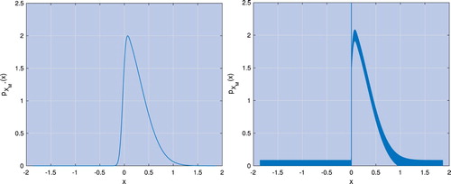
However, for the α-quantile options we price in this paper, we require the distribution of the maximum (minimum) for $n\ge 0$. As all Lévy processes have the property that $X\left(0\right)=0$, the value of the maximum for $n\ge 0$ cannot go below 0. Therefore obtaining $p_{X_M}(x,j)$ using the Spitzer-based scheme with the full number of dates alters the PDF so that it now has an abrupt discontinuity and a large spike at x = 0 as shown on the right-hand panel of figure 1. This spike corresponds to a single probability mass equal to ${\int }_{-\mathrm{\infty }}^0{p}_{X_M^{\prime }}(x,j)r\mathrm{d}x$. This can be understood by seeing that the cumulative distribution function (CDF) of $X_M\left(j\right)$ is (23) $P_{X_M}(x,j)=\left\{\begin{array}{ll}0& \mathrm{f}\mathrm{o}\mathrm{r}x<0\\ P\left(X_M^{\prime }\right(j)\le x)& \mathrm{f}\mathrm{o}\mathrm{r}x\ge 0.\end{array}\right.$(23) If $P\left(X_M^{\prime }\right(j)\le 0)\ne 0$, as is generally the case for Lévy processes, $P_{X_M}(x,j)$ has a jump at x = 0 of size $P(X_M^{\prime }\left(j\right)\le 0)={\int }_{-\mathrm{\infty }}^0{p}_{X_M^{\prime }}(x,j)\mathrm{d}x$. Thus when the CDF is differentiated to give the PDF $p_{X_M}(x,j)$, this will contain a probability mass at x = 0 of size ${\int }_{-\mathrm{\infty }}^0{p}_{X_M^{\prime }}(x,j)\mathrm{d}x$. The use of such mixed distributions is quite well established in the literature about the maxima and minima of processes; see e.g. (Feng and Linetsky 2009). It can be formalised denoting the probability mass with $\delta \left(x\right){\int }_{-\mathrm{\infty }}^0{p}_{X_M^{\prime }}(x^{\prime },j)\mathrm{d}{x}^{\prime }$ to give a continuous probability distribution which integrates to the expression for the CDF in equation (23(23) $P_{X_M}(x,j)=\left\{\begin{array}{ll}0& \mathrm{f}\mathrm{o}\mathrm{r}x<0\\ P\left(X_M^{\prime }\right(j)\le x)& \mathrm{f}\mathrm{o}\mathrm{r}x\ge 0.\end{array}\right.$(23) ). With respect to the pricing algorithm presented in section 3.1.1, one can also note that the regularity of the function ${\hat{p}}_{X_{\alpha }}$ depends on the Wiener–Hopf factors ${\mathrm{\Phi }}_{\oplus }(\xi ,q)$ and ${\mathrm{\Phi }}_{\ominus }(\xi ,q)$, which are smooth enough to permit the Fourier inversion; see e.g. (Eberlein et al. 2011).

The introduction of the discontinuity and spike has caused oscillations in the plot of the PDF via the Gibbs phenomenon. The discontinuity means that, as described for example by Boyd (2001) and Gottlieb and Shu (1997), we would no longer obtain exponential error convergence with grid size using these distributions to price options. We work around this with a spectral filter, as successfully implemented for Fourier-based option-pricing methods by Cui et al. (2017), Phelan et al. (2019) and Ruijter et al. (2015). In particular, we use an exponential filter of order 12 (Gottlieb and Shu 1997).

3.1.1. Pricing procedure for α-quantile options

We price a discretely monitored α-quantile option with a uniform monitoring interval $\mathrm{\Delta }t=T/N$ between N dates. The uniform interval is necessary to apply the z-transform, and it is one of the main assumptions to obtain a procedure whose computational cost is independent of the number of monitoring dates. As explained by Petrella and Kou (2004) in reference to the work on lookback options by Öhgren (2001), the method could be used to price at other monitoring dates if the previous maximum and minimum of the stock price can be ignored. Since the last assumption is strong, we wrote the whole article pricing the contract at time n = 0, i.e. the inception date is also when we start to measure the maximum/minimum.

In order to calculate the price of discretely monitored α-quantile options using the Fourier-z transform, we must express the time for the two independent random processes in terms of the number N of monitoring dates; given N, we round $j=\alpha N$ to the nearest integer (in our tests, we select α and N such that $\alpha N$ is an integer). The pricing procedure is then

1. Compute the characteristic function $\mathrm{\Psi }(\xi +i{\alpha }_{\mathrm{d}},\mathrm{\Delta }t)$ of the underlying transition density, where ${\alpha }_{\mathrm{d}}$ is the damping parameter introduced in section 2.

2. Use the Plemelj–Sokhotsky relations, equations (11(11) $\begin{array}{rl}\widehat{f_{l+}}\left(\xi \right)& =\frac{1}{2}\{\hat{f}\left(\xi \right)+e^{il\xi }i\mathcal{H}[{\mathrm{e}}^{-il\xi }\hat{f}\left(\xi \right)]\}\end{array}$(11) )–(12(12) $\begin{array}{rl}\widehat{f_{l-}}\left(\xi \right)& =\frac{1}{2}\{\hat{f}\left(\xi \right)-e^{il\xi }i\mathcal{H}[{\mathrm{e}}^{-il\xi }\hat{f}\left(\xi \right)]\}.\end{array}$(12) ), with the sinc-based fast Hilbert transform to factorise (24) $\begin{array}{rl}\mathrm{\Phi }(\xi ,q)& :=1-q\sigma \left(\xi /{\xi }_{max}\right)\mathrm{\Psi }(\xi +i{\alpha }_{\mathrm{d}},\mathrm{\Delta }t)\\ & ={\mathrm{\Phi }}_{\oplus }(\xi ,q){\mathrm{\Phi }}_{\ominus }(\xi ,q),\end{array}$(24) where $\sigma \left(\eta \right)$ is an exponential filter of order 12 as defined by Gottlieb and Shu (1997) and q is selected according to the criteria specified by Abate and Whitt (1992) for the inverse z-transform.

3. Calculate the Fourier-z transform of the PDF of the maximum $X_M$ and of the minimum $X_m$, (25) $\begin{array}{rl}{\widetilde{\stackrel{ˆ}{p}}}_{X_M}(\xi ,q)& =\frac{1}{{\mathrm{\Phi }}_{\oplus }(\xi ,q){\mathrm{\Phi }}_{\ominus }(0,q)}\end{array}$(25) (26) $\begin{array}{rl}{\widetilde{\stackrel{ˆ}{p}}}_{X_m}(\xi ,q)& =\frac{1}{{\mathrm{\Phi }}_{\oplus }(0,q){\mathrm{\Phi }}_{\ominus }(\xi ,q)}.\end{array}$(26)

4. Apply the inverse z-transform for j and N−j dates, respectively (27) $\begin{array}{rl}{\hat{p}}_{X_M}(\xi ,j)& ={\mathcal{Z}}_{q\to j}^{-1}\left[{\widetilde{\stackrel{ˆ}{p}}}_{X_M}(\xi ,q)\right]\end{array}$(27) (28) $\begin{array}{rl}{\hat{p}}_{X_m}(\xi ,N-j)& ={\mathcal{Z}}_{q\to N-j}^{-1}\left[{\widetilde{\stackrel{ˆ}{p}}}_{X_m}(\xi ,q)\right].\end{array}$(28)

5. Eliminate the numerical error in the characteristic functions of $X_M$ and $X_m$ that corresponds to a spurious imaginary part of the PDF to avoid its propagation in the next step, (29) $\begin{array}{rl}{\hat{p}}_{X_M}^{\mathrm{R}\mathrm{e}}(\xi ,j)& :={\mathcal{F}}_{x\to \xi }[\mathrm{R}\mathrm{e}{p}_{X_M}(x,j)]\\ & =\frac{1}{2}[{\hat{p}}_{X_M}(\xi ,j)+{\hat{p}}_{X_M}^{\ast }(-\xi ,j)]\end{array}$(29) (30) $\begin{array}{rl}{\hat{p}}_{X_m}^{\mathrm{R}\mathrm{e}}(\xi ,N-j)& :={\mathcal{F}}_{x\to \xi }[\mathrm{R}\mathrm{e}{p}_{X_m}(x,j)]\\ & =\frac{1}{2}[{\hat{p}}_{X_m}(\xi ,N-j)+{\hat{p}}_{X_m}^{\ast }(-\xi ,N-j)].\end{array}$(30)

6. Calculate the characteristic function of $X_{\alpha }$ at the monitoring date N, (31) ${\hat{p}}_{X_{\alpha }}(\xi ,N)={\hat{p}}_{X_M}^{\mathrm{R}\mathrm{e}}(\xi ,j){\hat{p}}_{X_m}^{\mathrm{R}\mathrm{e}}(\xi ,N-j).$(31)

7. Calculate the price of the discretely monitored α-quantile option at time 0, (32) $v(0,0)={\mathcal{F}}_{\xi \to x}^{-1}[\sigma \left(\xi /{\xi }_{max}\right){\hat{p}}_{X_{\alpha }}(\xi ,N){\hat{\phi }}^{\ast }\left(\xi \right)]\left(0\right),$(32) where $\sigma \left(\eta \right)$ is an exponential filter of order 12, as in Step (ii) above.

In the procedure above, Steps (i)–(iii) relate to the calculation of the Wiener–Hopf factors and the Spitzer identities for the maximum and minimum of a process, as described in equations (17(17) $\begin{array}{rl}{\widetilde{\stackrel{ˆ}{p}}}_{X_M}(\xi ,q)& =\frac{1}{{\mathrm{\Phi }}_{\oplus }(\xi ,q){\mathrm{\Phi }}_{\ominus }(0,q)}\end{array}$(17) ) and (18(18) $\begin{array}{rl}{\widetilde{\stackrel{ˆ}{p}}}_{X_m}(\xi ,q)& =\frac{1}{{\mathrm{\Phi }}_{\oplus }(0,q){\mathrm{\Phi }}_{\ominus }(\xi ,q)},\end{array}$(18) ). Steps (iv)–(vi) obtain the PDF of $X_{\alpha }\left(N\right)$ as described in equations (19(19) $\begin{array}{rl}{\hat{p}}_{X_M}(\xi ,j)& ={\mathcal{Z}}_{q\to j}^{-1}\left[{\widetilde{\stackrel{ˆ}{p}}}_{X_M}(\xi ,q)\right]\end{array}$(19) )–(22(22) ${\hat{p}}_{X_{\alpha }}(\xi ,N)={\hat{p}}_{X_M}(\xi ,j){\hat{p}}_{X_m}(\xi ,N-j).$(22) ) and Step (vii) uses the Plancherel relation, equation (3(3) $\begin{array}{rl}v(0,0)& ={\mathrm{e}}^{-rT}E[\phi \left(x\right(T\left)\right){\mathrm{e}}^{-{\alpha }_{\mathrm{d}}x\left(T\right)}|x\left(0\right)=0]\\ & ={\mathrm{e}}^{-rT}{\int }_{-\mathrm{\infty }}^{+\mathrm{\infty }}\phi \left(x\right){\mathrm{e}}^{-{\alpha }_{\mathrm{d}}x}p(x,T)\mathrm{d}x\\ & =\frac{{\mathrm{e}}^{-rT}}{2\pi }{\int }_{-\mathrm{\infty }}^{+\mathrm{\infty }}\hat{\phi }\left(\xi \right){\hat{p}}^{\ast }(\xi +i{\alpha }_{\mathrm{d}},T)\mathrm{d}\xi \\ & ={\mathrm{e}}^{-rT}{\mathcal{F}}_{\xi \to x}^{-1}\left[\hat{\phi }\left(\xi \right){\hat{p}}^{\ast }(\xi +i{\alpha }_{\mathrm{d}},T)\right]\left(0\right).\end{array}$(3) ), to obtain the final price.

3.2. Results for discretely monitored α-quantile options

We implemented the pricing method described above using the numerical procedure described step-by-step in Appendix 1. figure 2 shows results with $\alpha =0.75$ for N = 52, 252 and 1008 monitoring dates for the Gaussian, VG, and Merton jump-diffusion (MJD) processes.

Figure 2. Convergence of the pricing error with CPU time with the log-price of the underlying asset modelled by Gaussian (right), VG (centre) and Merton processes. For the Gaussian and Merton processes the log-price grid size range is $2^7-2^{12}$, and for the VG process the range is $2^8-2^{17}$.

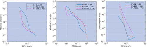
The error convergence for this method is extremely fast; we were able to achieve a CPU time of ${10}^{-2}$ seconds or less for an error of ${10}^{-8}$ using the Gaussian and Merton processes and ${10}^{-6}$ using the VG process. There are too few points before reaching the error floor of ${10}^{-11}$, caused by the inverse z-transform, to assess whether the error convergence is exponential or high-order polynomial. This is not a concern for using the method in practice, but a more accurate z-transform would allow us to understand the convergence better.

In table 1 we show the variation of the price with α for 252 monitoring dates (as expected the option price increases with α) and compare the results with those from three other pricing methods. We use two Monte Carlo methods. The first simulates N monitoring date paths and selects the jth smallest value. The second uses the same approach as (Ballotta and Kyprianou 2001) by combining the Monte Carlo simulation with the Dassios–Port–Wendel identity. Two independent paths of length $j\mathrm{\Delta }t$ and $(N-j)\mathrm{\Delta }t$ dates are simulated and the sum of their respective minimum and maximum is calculated to provide an estimate of the α-quantile. Further details about this Monte Carlo scheme are included in Appendix 3. The third comparison is with a recursive method drawn from Feng and Linetsky (2009) and Green (2009). It uses the property that for a random walk (33) $X\left(t_n\right)=X\left(t_{n-1}\right)+Q_n,X\left(0\right)=0,$(33) where $Q_n$ are independent and identically distributed random variables with PDF $p(x,\mathrm{\Delta }t)$, $X_M\left(t_n\right)$, defined as the maximum value of $X\left(t_n\right)$ between the times $t_0=0$ and $t_n=n\mathrm{\Delta }T$, has the same probability distribution as the process $R_M\left(t_n\right)$ defined recursively as (34) $R_M\left(t_n\right)=max\left(R_M\right(t_{n-1})+Q_n,0),R_M\left(0\right)=0,$(34) and $X_m\left(t_n\right)$ has the same probability distribution as the process $R_m\left(t_n\right)$ defined recursively as (35) $R_m\left(t_n\right)=min\left(R_m\right(t_{n-1})+Q_n,0),R_m\left(0\right)=0.$(35) This gives recursive relationships for the PDFs of $X_M$ and $X_m$, (36) $\begin{array}{rl}{p}_M(x,t_n)& ={\int }_0^{\mathrm{\infty }}{p}_M(x^{\prime },t_{n-1})p(x-x^{\prime },\mathrm{\Delta }t)\mathrm{d}{x}^{\prime },\\ p_M(x,0)& =\delta \left(x\right)\end{array}$(36) (37) $\begin{array}{rl}{p}_m(x,t_n)& ={\int }_{-\mathrm{\infty }}^0{p}_m(x^{\prime },t_{n-1})p(x-x^{\prime },\mathrm{\Delta }t)\mathrm{d}{x}^{\prime },\\ p_m(x,0)& =\delta \left(x\right).\end{array}$(37) This can be implemented in the Fourier domain using the Plemelj–Sokhotsky relations, equations (11(11) $\begin{array}{rl}\widehat{f_{l+}}\left(\xi \right)& =\frac{1}{2}\{\hat{f}\left(\xi \right)+e^{il\xi }i\mathcal{H}[{\mathrm{e}}^{-il\xi }\hat{f}\left(\xi \right)]\}\end{array}$(11) )–(12(12) $\begin{array}{rl}\widehat{f_{l-}}\left(\xi \right)& =\frac{1}{2}\{\hat{f}\left(\xi \right)-e^{il\xi }i\mathcal{H}[{\mathrm{e}}^{-il\xi }\hat{f}\left(\xi \right)]\}.\end{array}$(12) ), and the sinc-based fast Hilbert transform in a similar way as done for barrier options by Feng and Linetsky (2008) and Fusai et al. (2016), (38) $\begin{array}{rl}{\hat{p}}_M(\xi ,t_n)& =\frac{1}{2}({\hat{p}}_M(\xi ,t_{n-1})\mathrm{\Psi }(\xi ,\mathrm{\Delta }t)\\ & +\mathcal{H}\left[{\hat{p}}_M(\xi ,t_{n-1})\mathrm{\Psi }(\xi ,\mathrm{\Delta }t)\right]),\end{array}$(38) (39) $\begin{array}{rl}{\hat{p}}_m(\xi ,t_n)& =\frac{1}{2}({\hat{p}}_m(\xi ,t_{n-1})\mathrm{\Psi }(\xi ,\mathrm{\Delta }t)\\ & -\mathcal{H}\left[{\hat{p}}_m(\xi ,t_{n-1})\mathrm{\Psi }(\xi ,\mathrm{\Delta }t)\right]),\end{array}$(39) where $\mathrm{\Psi }(\xi ,\mathrm{\Delta }t)={\mathcal{F}}_{x\to \xi }\left[p\right(x,\mathrm{\Delta }t\left)\right]$ is the characteristic function of $Q_n$. The characteristic functions of $X_M$ and $X_m$ calculated in this way are then multiplied as in equation (22(22) ${\hat{p}}_{X_{\alpha }}(\xi ,N)={\hat{p}}_{X_M}(\xi ,j){\hat{p}}_{X_m}(\xi ,N-j).$(22) ).

Table 1. Price of an α-quantile option with 252 monitoring dates computed with our new method, the recursion method, Monte Carlo, and Monte Carlo combined with the Dassios–Port–Wendel identity.

			Monte Carlo		Monte Carlo + DPW
α	Spitzer price	recursion price	price	std dev	price	std dev
Gaussian
2/3	0.20847221	0.20847221	0.208438	3.8E−5	0.208460	3.8E−5
3/4	0.24346206	0.24346206	0.243491	4.1E−5	0.243440	4.1E−5
5/6	0.28541044	0.28541044	0.285367	4.5E−5	0.285445	4.5E−5
Variance gamma
2/3	0.15893822	0.15893822	0.158933	4.0E−5	0.158915	4.0E−5
3/4	0.17649028	0.17649028	0.176453	4.3E−5	0.176493	4.3E−5
5/6	0.19604275	0.19604275	0.196066	4.4E−5	0.196050	4.4E−5
Merton jump-diffusion
2/3	0.15957162	0.15957162	0.159540	3.9E−5	0.159566	3.9E−5
3/4	0.17757317	0.17757317	0.177592	4.1E−5	0.177600	4.1E−5
5/6	0.19776625	0.19776625	0.197760	4.3E−5	0.197724	4.3E−5

Note: Both the Spitzer and the recursion method use $2^{16}$ log-price grid points.

Table 1 shows that the prices calculated using our new method are consistent with both Monte Carlo methods and match the recursion method to 8 decimal places. We can therefore be confident that our new method gives highly accurate results with very short CPU times as shown in figure 2.

4. Perpetual Bermudan options

Bermudan options have the same payoff as European options, but they can be exercised at a discrete set of intermediate dates rather than only at the final expiry date. They can be thought of as a discrete version of American options and, indeed, the price of a Bermudan option is often used as an approximation for the price of an American option; see e.g. (Feng and Lin 2013). Perpetual Bermudan and American options have no expiry and therefore ‘live’ until they are exercised. Pricing perpetual options is an easier problem than the valuation of those with finite expiry because the infinite time horizon makes the optimal exercise boundary a constant rather than a function of time. Indeed, closed-form formulas exist for perpetual American options with simple processes, whereas there are none for finite-expiry options.

We look at two methods for pricing perpetual Bermudan options. Firstly we implement the method by Green (2009) which uses residue calculus. We also implement a new method which uses Spitzer identities and show a novel way to calculate the optimal exercise boundary. We specify new numerical truncation bounds for the log-price domain; they are required because of the infinite time horizon.

Both methods require the probability distribution of the current value of a process, subject to the path not having crossed a lower barrier l, i.e. (40) $p_l(x,n)\mathrm{d}x=P\left[X_n\in (x,x+\mathrm{d}x]\cap \underset{j<n}{min}{X}_j>l\right].$(40) Using techniques from complex analysis, Green (2009) and Green et al. (2010) showed that this can be expressed using the Spitzer identities as (41) $\begin{array}{rl}{p}_l(x,n)& =\left\{\begin{array}{ll}{\mathcal{Z}}_{q\to n}^{-1}\left[{\mathcal{F}}_{\xi \to x}^{-1}\left[\frac{P_{l+}(\xi ,q)}{{\mathrm{\Phi }}_{\oplus }(\xi ,q)}\right]\right],& x\ge l,\\ {\mathcal{Z}}_{q\to n}^{-1}\left[{\mathcal{F}}_{\xi \to x}^{-1}\left[P_{l-}(\xi ,q){\mathrm{\Phi }}_{\ominus }(\xi ,q)\right]\right],& x<l,\end{array}\right.\end{array}$(41) where ${\mathrm{\Phi }}_{\oplus }(\xi ,q)$ and ${\mathrm{\Phi }}_{\ominus }(\xi ,q)$ are as defined in section 3.1 and $P_{l+}$ and $P_{l-}$ are calculated decomposing $P=1/{\mathrm{\Phi }}_{\ominus }(\xi ,q)$ around l.

The order of the inverse transforms can be swapped. The method we develop here for pricing perpetual Bermudan options calculates the expected return from exercising the option at each monitoring date and sums this over all monitoring dates. Therefore we use the form of the Spitzer identity in equation (41(41) $\begin{array}{rl}{p}_l(x,n)& =\left\{\begin{array}{ll}{\mathcal{Z}}_{q\to n}^{-1}\left[{\mathcal{F}}_{\xi \to x}^{-1}\left[\frac{P_{l+}(\xi ,q)}{{\mathrm{\Phi }}_{\oplus }(\xi ,q)}\right]\right],& x\ge l,\\ {\mathcal{Z}}_{q\to n}^{-1}\left[{\mathcal{F}}_{\xi \to x}^{-1}\left[P_{l-}(\xi ,q){\mathrm{\Phi }}_{\ominus }(\xi ,q)\right]\right],& x<l,\end{array}\right.\end{array}$(41) ) for x<l. That is, for each discretely spaced exercise date, we require the distribution of $X\left(n\right)$ subject to n being the first monitoring date when it has gone below the optimal exercise boundary. 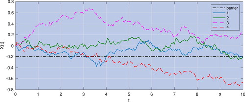If the underlying has gone below the optimal exercise boundary at a previous monitoring date $(j\le n-1)$ then the option would have exercised at date j and this path will not contribute to the expected return at date n. Conversely for paths that are above the optimal exercise boundary at date n, we would not choose to exercise the option and therefore these paths will also not contribute to the expected return at date n. In order to maintain the link to the work using Spitzer identities to price barrier options, for example by Fusai et al. (2016), we denote the log of the optimal exercise boundary by l which is used for the lower log-barrier in the work on barrier options. Several different possible paths are illustrated in figure 3 for a process with 10 monitoring dates and l = −0.2. The value of $X\left(10\right)$ for paths 1 and 2 would contribute to the required distribution as the paths stay above l for monitoring dates 0–9, but go below l at the monitoring date 10. Path 3 does not count towards the distribution as it is above l at the 10th monitoring date and path 4 does not count as it goes below l at an earlier monitoring date.

Figure 3. Discretely monitored continuous random paths with 10 monitoring dates and $\mathrm{\Delta }t=1$. Only the paths that stay above the barrier (dot-dashed line) at monitoring dates 0–9 and descend below the barrier at date 10 contribute to the target distribution; they are indicated with continuous lines. The paths which are on or below the barrier for at least one monitoring date between 0 and 9, or are above the barrier at date 10 are not included in the target distribution and are indicated with dashed lines.

4.1. Green's residue method

We briefly recapitulate the method described by Green (2009) to provide a background to the results from our numerical implementation and also because we re-use some of the same techniques in deriving the new Spitzer-based method described in section 4.2. The scheme is based on a combination of a first-touch option paying K−D, where K is the strike, and an overshoot option which pays the difference between a barrier D and the underlying asset $S\left(t\right)=S_0{e}^{X\left(t\right)}$ the first time the barrier is crossed. A first-touch option requires the probability that the first time the underlying asset crosses the barrier l is time $n\mathrm{\Delta }t$, i.e. (42) $P[{\tau }_l=n\mathrm{\Delta }t]={\int }_{-\mathrm{\infty }}^l{p}_l(x,n)\mathrm{d}x.$(42) Substituting $p_l(x,n)={\mathcal{Z}}_{q\to n}^{-1}\left[{\mathcal{F}}_{\xi \to x}^{-1}\right[P_{l-}(\xi ,q){\mathrm{\Phi }}_{\ominus }(\xi ,q)\left]\right]$ from equation (41(41) $\begin{array}{rl}{p}_l(x,n)& =\left\{\begin{array}{ll}{\mathcal{Z}}_{q\to n}^{-1}\left[{\mathcal{F}}_{\xi \to x}^{-1}\left[\frac{P_{l+}(\xi ,q)}{{\mathrm{\Phi }}_{\oplus }(\xi ,q)}\right]\right],& x\ge l,\\ {\mathcal{Z}}_{q\to n}^{-1}\left[{\mathcal{F}}_{\xi \to x}^{-1}\left[P_{l-}(\xi ,q){\mathrm{\Phi }}_{\ominus }(\xi ,q)\right]\right],& x<l,\end{array}\right.\end{array}$(41) ) into this and taking the expectation over all dates, Green (2009) obtains the price of the option as (43) $\begin{array}{r}{v}_{\mathrm{F}}(0,0)=(K-D)\sum _{n=1}^{\mathrm{\infty }}{\mathrm{e}}^{-rn\mathrm{\Delta }t}{\mathcal{Z}}_{q\to n}^{-1}[P_{l-}(0,q){\mathrm{\Phi }}_{\ominus }(0,q)].\end{array}$(43) The next insight by Green (2009) is that the summation and inverse z-transform cancel each other if we use $q={\mathrm{e}}^{-r\mathrm{\Delta }t}$ because the summation equates to a forward z-transform. Then the price for a first-touch option is (44) $v_{\mathrm{F}}(0,0)=(K-D)P_{l-}\left(0,{\mathrm{e}}^{-r\mathrm{\Delta }t}\right){\mathrm{\Phi }}_{\ominus }\left(0,{\mathrm{e}}^{-r\mathrm{\Delta }t}\right).$(44) The value of the payoff of an overshoot option at date n is the expected overshoot $D-S\left(t_n\right)$ conditional on n being the first date when the underlying asset process falls below l, ${\tau }_l$ is (45) $\begin{array}{rl}& E\left[{\mathrm{e}}^{-r{\tau }_l}\right(D-S\left({\tau }_l\right))|{\tau }_l=n\mathrm{\Delta }t]\\ & ={\mathrm{e}}^{-rn\mathrm{\Delta }t}{\int }_{-\mathrm{\infty }}^l(D-S_0{e}^x)p_l(x,n)\mathrm{d}x.\end{array}$(45) We calculate the option value by using the tower property to take the expectation over all discrete monitoring dates, and we substitute $p_l(x,n)={\mathcal{Z}}_{q\to n}^{-1}\left[{\mathcal{F}}_{\xi \to x}^{-1}\right[P_{l-}(\xi ,q){\mathrm{\Phi }}_{\ominus }(\xi ,q)\left]\right]$ to obtain (46) $\begin{array}{rl}{v}_{\mathrm{O}}(0,0)& =\sum _{n=1}^{\mathrm{\infty }}{\mathrm{e}}^{-rn\mathrm{\Delta }t}{\int }_{-\mathrm{\infty }}^l(D-S_0{e}^x){\mathcal{Z}}_{q\to n}^{-1}\\ & \times \left[{\mathcal{F}}_{\xi \to x}^{-1}\left[P_{l-}(\xi ,q){\mathrm{\Phi }}_{\ominus }(\xi ,q)\right]\right]\mathrm{d}x\\ & =\frac{1}{2\pi }{\int }_{-\mathrm{\infty }}^{+\mathrm{\infty }}\hat{\phi }(-\xi )P_{l-}(\xi ,{\mathrm{e}}^{-r\mathrm{\Delta }t}){\mathrm{\Phi }}_{\ominus }(\xi ,{\mathrm{e}}^{-r\mathrm{\Delta }t})\mathrm{d}x.\end{array}$(46) In the first line we set $q={\mathrm{e}}^{-r\mathrm{\Delta }t}$ to cancel the inverse z-transform as before; in the second line we use the Plancherel relation to move into the Fourier domain. Using equation (5(5) $\begin{array}{rl}\hat{\phi }\left(\xi \right)& =S_0\left(\frac{e^{(1+i\xi +{\alpha }_{\mathrm{d}})a}-e^{(1+i\xi +{\alpha }_{\mathrm{d}})b}}{1+i\xi +{\alpha }_{\mathrm{d}}}\right.\\ & -\left.\frac{e^{k+(i\xi +{\alpha }_{\mathrm{d}})a}-e^{k+(i\xi +{\alpha }_{\mathrm{d}})b}}{i\xi +{\alpha }_{\mathrm{d}}}\right),\end{array}$(5) ) for $\hat{\phi }\left(\xi \right)$ for a put option with $a=-\mathrm{\infty }$, b = l, k = l, ${\alpha }_{\mathrm{d}}>0$ and solving via the residue method, (47) $\begin{array}{rl}{v}_{\mathrm{O}}(0,0)& =-\frac{D}{2\pi }{\int }_{-\mathrm{\infty }}^{+\mathrm{\infty }}\frac{P_{l-}(\xi ,{\mathrm{e}}^{-r\mathrm{\Delta }t}){\mathrm{\Phi }}_{\ominus }(\xi ,{\mathrm{e}}^{-r\mathrm{\Delta }t})}{{\xi }^2+i\xi }\mathrm{d}x\\ & =D{P}_{l-}(0,{\mathrm{e}}^{-r\mathrm{\Delta }t}){\mathrm{\Phi }}_{\ominus }(0,{\mathrm{e}}^{-r\mathrm{\Delta }t})\\ & -D{P}_{l-}(-i,{\mathrm{e}}^{-r\mathrm{\Delta }t}){\mathrm{\Phi }}_{\ominus }(-i,{\mathrm{e}}^{-r\mathrm{\Delta }t}).\end{array}$(47) Choosing the barrier l as the optimal exercise boundary, the price $v_{\mathrm{B}}$ of a perpetual Bermudan option is the sum of the price $v_{\mathrm{F}}$ of a first-touch option with payoff K−D, equation (43(43) $\begin{array}{r}{v}_{\mathrm{F}}(0,0)=(K-D)\sum _{n=1}^{\mathrm{\infty }}{\mathrm{e}}^{-rn\mathrm{\Delta }t}{\mathcal{Z}}_{q\to n}^{-1}[P_{l-}(0,q){\mathrm{\Phi }}_{\ominus }(0,q)].\end{array}$(43) ), and the price of an overshoot option, equation (47(47) $\begin{array}{rl}{v}_{\mathrm{O}}(0,0)& =-\frac{D}{2\pi }{\int }_{-\mathrm{\infty }}^{+\mathrm{\infty }}\frac{P_{l-}(\xi ,{\mathrm{e}}^{-r\mathrm{\Delta }t}){\mathrm{\Phi }}_{\ominus }(\xi ,{\mathrm{e}}^{-r\mathrm{\Delta }t})}{{\xi }^2+i\xi }\mathrm{d}x\\ & =D{P}_{l-}(0,{\mathrm{e}}^{-r\mathrm{\Delta }t}){\mathrm{\Phi }}_{\ominus }(0,{\mathrm{e}}^{-r\mathrm{\Delta }t})\\ & -D{P}_{l-}(-i,{\mathrm{e}}^{-r\mathrm{\Delta }t}){\mathrm{\Phi }}_{\ominus }(-i,{\mathrm{e}}^{-r\mathrm{\Delta }t}).\end{array}$(47) ), i.e. (48) $\begin{array}{rl}{v}_{\mathrm{B}}(0,0)& =v_{\mathrm{F}}(0,0)+v_{\mathrm{O}}(0,0)=K{P}_{l-}(0,{\mathrm{e}}^{-r\mathrm{\Delta }t}){\mathrm{\Phi }}_{\ominus }(0,{\mathrm{e}}^{-r\mathrm{\Delta }t})\\ & -D{P}_{l-}(-i,{\mathrm{e}}^{-r\mathrm{\Delta }t}){\mathrm{\Phi }}_{\ominus }(-i,{\mathrm{e}}^{-r\mathrm{\Delta }t}).\end{array}$(48) Green (2009) showed that, as the optimal exercise boundary gives a maximum price, solving $\mathrm{\partial }{v}_{\mathrm{B}}(0,0)/\mathrm{\partial }D=0$ for D gives the optimal exercise boundary, (49) $D_{\mathrm{o}\mathrm{p}\mathrm{t}}=K\frac{{\mathrm{\Phi }}_{\ominus }(0,{\mathrm{e}}^{-r\mathrm{\Delta }t})}{{\mathrm{\Phi }}_{\ominus }(-i,{\mathrm{e}}^{-r\mathrm{\Delta }t})}.$(49) Then, defining $l_{\mathrm{o}\mathrm{p}\mathrm{t}}:=\log \left(D_{\mathrm{o}\mathrm{p}\mathrm{t}}/S_0\right)$, we obtain the price of a perpetual Bermudan option, (50) $\begin{array}{r}{v}_{\mathrm{B}}(0,0)=K{\mathrm{\Phi }}_{\ominus }(0,{\mathrm{e}}^{-r\mathrm{\Delta }t})\left[P_{l_{\mathrm{o}\mathrm{p}\mathrm{t}}-}\right(0,{\mathrm{e}}^{-r\mathrm{\Delta }t}\left)-P_{l_{\mathrm{o}\mathrm{p}\mathrm{t}}-}\right(-i,{\mathrm{e}}^{-r\mathrm{\Delta }t}\left)\right].\end{array}$(50) Therefore, we have proved the following result.

Theorem 4.1

Let $X\left(t\right)$ be a Lévy process and ${\alpha }_{\mathrm{d}}$ be an appropriate damping parameter.¹ Then the price at time t = 0 of a perpetual Bermudan put option on the underlying asset $S\left(t\right)=S_0{e}^{X\left(t\right)}$ with strike K and the set $\{j\mathrm{\Delta }t{\}}_{j\in \mathbb{N}}$ of possible early exercise dates is given by $v_{\mathrm{B}}(0,0)$ provided in equation (50(50) $\begin{array}{r}{v}_{\mathrm{B}}(0,0)=K{\mathrm{\Phi }}_{\ominus }(0,{\mathrm{e}}^{-r\mathrm{\Delta }t})\left[P_{l_{\mathrm{o}\mathrm{p}\mathrm{t}}-}\right(0,{\mathrm{e}}^{-r\mathrm{\Delta }t}\left)-P_{l_{\mathrm{o}\mathrm{p}\mathrm{t}}-}\right(-i,{\mathrm{e}}^{-r\mathrm{\Delta }t}\left)\right].\end{array}$(50) ), where $l_{\mathrm{o}\mathrm{p}\mathrm{t}}=\log \left(D_{\mathrm{o}\mathrm{p}\mathrm{t}}/S_0\right),$ $D_{\mathrm{o}\mathrm{p}\mathrm{t}}$ is given by equation (49(49) $D_{\mathrm{o}\mathrm{p}\mathrm{t}}=K\frac{{\mathrm{\Phi }}_{\ominus }(0,{\mathrm{e}}^{-r\mathrm{\Delta }t})}{{\mathrm{\Phi }}_{\ominus }(-i,{\mathrm{e}}^{-r\mathrm{\Delta }t})}.$(49) ), ${\mathrm{\Phi }}_{\ominus }(\xi ,q)$ is given by equation (24(24) $\begin{array}{rl}\mathrm{\Phi }(\xi ,q)& :=1-q\sigma \left(\xi /{\xi }_{max}\right)\mathrm{\Psi }(\xi +i{\alpha }_{\mathrm{d}},\mathrm{\Delta }t)\\ & ={\mathrm{\Phi }}_{\oplus }(\xi ,q){\mathrm{\Phi }}_{\ominus }(\xi ,q),\end{array}$(24) ), and $P_{l_{\mathrm{o}\mathrm{p}\mathrm{t}}-}(\xi ,q)$ is calculated decomposing $P=1/{\mathrm{\Phi }}_{\ominus }(\xi ,q)$ around $l_{\mathrm{o}\mathrm{p}\mathrm{t}}$.

For the optimal exercise log-boundary we chose the symbol $l_{\mathrm{o}\mathrm{p}\mathrm{t}}$ rather than $d_{\mathrm{o}\mathrm{p}\mathrm{t}}$ by analogy to the lower log-barrier l in the work on barrier options of Fusai et al. (2016), as will become clear in the next subsection.

4.2. New formulation based on Spitzer identities

The method by Green described in section 4.1 is very elegant mathematically, but does not particularly lend itself to an intuitive understanding. Therefore we also devised an alternative method for pricing perpetual Bermudan options, including a new way of calculating the optimal exercise boundary.

We first recognise that the expected return from exercising a perpetual Bermudan put at monitoring date n, subject to the underlying asset price being below the optimal exercise boundary $l_{\mathrm{o}\mathrm{p}\mathrm{t}}$, can be expressed as (51) $\begin{array}{r}E\left[{\mathrm{e}}^{-rn\mathrm{\Delta }t}\right(K-S\left(t_n\right){)}^{+}]={\mathrm{e}}^{-rn\mathrm{\Delta }t}{\int }_{-\mathrm{\infty }}^l(K-S_0{e}^x\left)p_{l_{\mathrm{o}\mathrm{p}\mathrm{t}}}\right(x,n)\mathrm{d}x.\end{array}$(51) To obtain the value of the option we sum over all monitoring dates; substituting ${\widetilde{\stackrel{ˆ}{p}}}_{l_{\mathrm{o}\mathrm{p}\mathrm{t}}}(\xi ,q)=P_{l_{\mathrm{o}\mathrm{p}\mathrm{t}}-}(\xi ,q){\mathrm{\Phi }}_{\ominus }(\xi ,q)$, (52) $\begin{array}{rl}{v}_{\mathrm{B}}(0,0)& =\sum _{n=1}^{\mathrm{\infty }}{\mathrm{e}}^{-rn\mathrm{\Delta }t}{\int }_{-\mathrm{\infty }}^l(K-S_0{e}^x){\mathcal{Z}}_{q\to n}^{-1}\\ & \times \left[{\mathcal{F}}_{\xi \to x}^{-1}[{\widetilde{\stackrel{ˆ}{p}}}_{l_{\mathrm{o}\mathrm{p}\mathrm{t}}}(\xi ,q)]\right]\mathrm{d}x.\end{array}$(52) We can again use the idea by Green (2009) of using $q={\mathrm{e}}^{-r\mathrm{\Delta }t}$ so that the summation cancels with the inverse z-transform to give (53) $v_{\mathrm{B}}(0,0)={\int }_{-\mathrm{\infty }}^l(K-S_0{e}^x){\mathcal{F}}_{\xi \to x}^{-1}[{\widetilde{\stackrel{ˆ}{p}}}_{l_{\mathrm{o}\mathrm{p}\mathrm{t}}}(\xi ,{\mathrm{e}}^{-r\mathrm{\Delta }t})]\mathrm{d}x.$(53) This integral can be expressed in the Fourier domain using the Plancherel relation, (54) $\begin{array}{rl}{v}_{\mathrm{B}}(0,0)& =\frac{1}{2\pi }{\int }_{-\mathrm{\infty }}^{+\mathrm{\infty }}{\hat{\phi }}^{\ast }\left(\xi \right){\widetilde{\stackrel{ˆ}{p}}}_{l_{\mathrm{o}\mathrm{p}\mathrm{t}}}(\xi ,{\mathrm{e}}^{-r\mathrm{\Delta }t})\mathrm{d}x\\ & ={\mathcal{F}}_{\xi \to x}^{-1}[{\hat{\phi }}^{\ast }\left(\xi \right){\widetilde{\stackrel{ˆ}{p}}}_{l_{\mathrm{o}\mathrm{p}\mathrm{t}}}(\xi ,{\mathrm{e}}^{-r\mathrm{\Delta }t})]\left(0\right),\end{array}$(54) where $\phi \left(\xi \right)$ is the damped payoff for a put option, equation (4(4) $\phi \left(x\right)=e^{{\alpha }_{\mathrm{d}}x}{S}_0\left(\theta \right(e^x-e^k\left){)}^{+}{\mathbf{1}}_{(l,u)}\right(x),$(4) ), with $l=l_{\mathrm{o}\mathrm{p}\mathrm{t}}$.

For this method, the calculation of the optimal exercise boundary is based on the idea that if the underlying asset is exactly at the optimal exercise boundary, i.e. $S_0=D_{\mathrm{o}\mathrm{p}\mathrm{t}}$, then the value of the payoff from exercising the option is equal to the expected value from continuing to hold the option. Furthermore, the log-boundary used to calculate ${\widetilde{\stackrel{ˆ}{p}}}_{l_{\mathrm{o}\mathrm{p}\mathrm{t}}}(\xi ,q)=P_{l_{\mathrm{o}\mathrm{p}\mathrm{t}}-}(\xi ,q){\mathrm{\Phi }}_{\ominus }(\xi ,q)$ is $l_{\mathrm{o}\mathrm{p}\mathrm{t}}=\log \left(D_{\mathrm{o}\mathrm{p}\mathrm{t}}/S_0\right)=0$, so that we can rewrite equation (51(51) $\begin{array}{r}E\left[{\mathrm{e}}^{-rn\mathrm{\Delta }t}\right(K-S\left(t_n\right){)}^{+}]={\mathrm{e}}^{-rn\mathrm{\Delta }t}{\int }_{-\mathrm{\infty }}^l(K-S_0{e}^x\left)p_{l_{\mathrm{o}\mathrm{p}\mathrm{t}}}\right(x,n)\mathrm{d}x.\end{array}$(51) ) as (55) $\begin{array}{rl}{v}_{\mathrm{B},S_0=D_{\mathrm{o}\mathrm{p}\mathrm{t}}}(0,0)& ={\int }_{-\mathrm{\infty }}^0(K-S_0{e}^x){\mathcal{F}}_{\xi \to x}^{-1}\\ & \times [P_{0-}(\xi ,{\mathrm{e}}^{-r\mathrm{\Delta }t}){\mathrm{\Phi }}_{\ominus }(\xi ,{\mathrm{e}}^{-r\mathrm{\Delta }t})]\mathrm{d}x\\ & ={\mathcal{F}}_{\xi \to x}^{-1}[{\hat{\phi }}^{\ast }\left(\xi \right)P_{0-}(\xi ,{\mathrm{e}}^{-r\mathrm{\Delta }t}){\mathrm{\Phi }}_{\ominus }(\xi ,{\mathrm{e}}^{-r\mathrm{\Delta }t})]\left(0\right).\end{array}$(55) If we differentiate the expression on the first line of equation (55(55) $\begin{array}{rl}{v}_{\mathrm{B},S_0=D_{\mathrm{o}\mathrm{p}\mathrm{t}}}(0,0)& ={\int }_{-\mathrm{\infty }}^0(K-S_0{e}^x){\mathcal{F}}_{\xi \to x}^{-1}\\ & \times [P_{0-}(\xi ,{\mathrm{e}}^{-r\mathrm{\Delta }t}){\mathrm{\Phi }}_{\ominus }(\xi ,{\mathrm{e}}^{-r\mathrm{\Delta }t})]\mathrm{d}x\\ & ={\mathcal{F}}_{\xi \to x}^{-1}[{\hat{\phi }}^{\ast }\left(\xi \right)P_{0-}(\xi ,{\mathrm{e}}^{-r\mathrm{\Delta }t}){\mathrm{\Phi }}_{\ominus }(\xi ,{\mathrm{e}}^{-r\mathrm{\Delta }t})]\left(0\right).\end{array}$(55) ) with respect to $S_0$, we obtain (56) $\begin{array}{rl}\frac{\mathrm{\partial }{v}_{\mathrm{B},S_0=D_{\mathrm{o}\mathrm{p}\mathrm{t}}}(0,0)}{\mathrm{\partial }{S}_0}& =-{\int }_{-\mathrm{\infty }}^0{e}^x{\mathcal{F}}_{\xi \to x}^{-1}\\ & \times [P_{0-}(\xi ,{\mathrm{e}}^{-r\mathrm{\Delta }t}){\mathrm{\Phi }}_{\ominus }(\xi ,{\mathrm{e}}^{-r\mathrm{\Delta }t})]\mathrm{d}x,\end{array}$(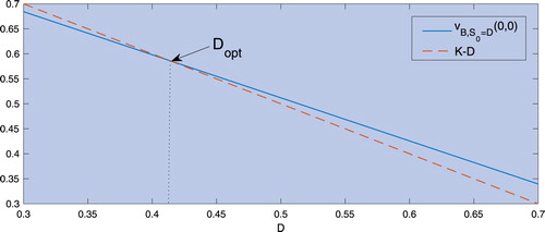56) which is constant. Therefore, if we plot $v_{\mathrm{B},S_0=D}(0,0)$ against $S_0=D$, we obtain a straight line, and the point where this line crosses the non-zero part of the payoff function $(K-S_0{)}^{+}$, i.e. $K-S_0$ for $S_0<K$, represents the optimal exercise boundary. This is illustrated in figure 4. Thus, by calculating equation (55(55) $\begin{array}{rl}{v}_{\mathrm{B},S_0=D_{\mathrm{o}\mathrm{p}\mathrm{t}}}(0,0)& ={\int }_{-\mathrm{\infty }}^0(K-S_0{e}^x){\mathcal{F}}_{\xi \to x}^{-1}\\ & \times [P_{0-}(\xi ,{\mathrm{e}}^{-r\mathrm{\Delta }t}){\mathrm{\Phi }}_{\ominus }(\xi ,{\mathrm{e}}^{-r\mathrm{\Delta }t})]\mathrm{d}x\\ & ={\mathcal{F}}_{\xi \to x}^{-1}[{\hat{\phi }}^{\ast }\left(\xi \right)P_{0-}(\xi ,{\mathrm{e}}^{-r\mathrm{\Delta }t}){\mathrm{\Phi }}_{\ominus }(\xi ,{\mathrm{e}}^{-r\mathrm{\Delta }t})]\left(0\right).\end{array}$(55) ) for two values of $S_0$, say $S_0=D_1$ and $S_0=D_2$, we obtain the corresponding straight line with slope m and intercept c. We then calculate the optimal exercise boundary $D_{\mathrm{o}\mathrm{p}\mathrm{t}}$, corresponding to the point where the lines cross, as (57) $D_{\mathrm{o}\mathrm{p}\mathrm{t}}=\frac{K-c}{m+1}.$(57) Therefore, we have proved the following result.

Theorem 4.2

Let $X\left(t\right)$ be a Lévy process and ${\alpha }_{\mathrm{d}}$ be an appropriate damping parameter. Then the price at time t = 0 of a perpetual Bermudan put option on the underlying asset $S\left(t\right)=S_0{e}^{X\left(t\right)}$ with strike K and the set $\{j\mathrm{\Delta }t{\}}_{j\in \mathbb{N}}$ of possible early exercise dates is given by $v_{\mathrm{B}}(0,0)$ provided in equation (54(54) $\begin{array}{rl}{v}_{\mathrm{B}}(0,0)& =\frac{1}{2\pi }{\int }_{-\mathrm{\infty }}^{+\mathrm{\infty }}{\hat{\phi }}^{\ast }\left(\xi \right){\widetilde{\stackrel{ˆ}{p}}}_{l_{\mathrm{o}\mathrm{p}\mathrm{t}}}(\xi ,{\mathrm{e}}^{-r\mathrm{\Delta }t})\mathrm{d}x\\ & ={\mathcal{F}}_{\xi \to x}^{-1}[{\hat{\phi }}^{\ast }\left(\xi \right){\widetilde{\stackrel{ˆ}{p}}}_{l_{\mathrm{o}\mathrm{p}\mathrm{t}}}(\xi ,{\mathrm{e}}^{-r\mathrm{\Delta }t})]\left(0\right),\end{array}$(54) ), where $l_{\mathrm{o}\mathrm{p}\mathrm{t}}=\log \left(D_{\mathrm{o}\mathrm{p}\mathrm{t}}/S_0\right)$, $D_{\mathrm{o}\mathrm{p}\mathrm{t}}$ is the unique solution of $v_{\mathrm{B},S_0=D_{\mathrm{o}\mathrm{p}\mathrm{t}}}(0,0)=K-D_{\mathrm{o}\mathrm{p}\mathrm{t}},$ ${\widetilde{\stackrel{ˆ}{p}}}_{l_{\mathrm{o}\mathrm{p}\mathrm{t}}}(\xi ,q)=P_{l_{\mathrm{o}\mathrm{p}\mathrm{t}}-}(\xi ,q){\mathrm{\Phi }}_{\ominus }(\xi ,q)$ with the left-hand side given by equation (55(55) $\begin{array}{rl}{v}_{\mathrm{B},S_0=D_{\mathrm{o}\mathrm{p}\mathrm{t}}}(0,0)& ={\int }_{-\mathrm{\infty }}^0(K-S_0{e}^x){\mathcal{F}}_{\xi \to x}^{-1}\\ & \times [P_{0-}(\xi ,{\mathrm{e}}^{-r\mathrm{\Delta }t}){\mathrm{\Phi }}_{\ominus }(\xi ,{\mathrm{e}}^{-r\mathrm{\Delta }t})]\mathrm{d}x\\ & ={\mathcal{F}}_{\xi \to x}^{-1}[{\hat{\phi }}^{\ast }\left(\xi \right)P_{0-}(\xi ,{\mathrm{e}}^{-r\mathrm{\Delta }t}){\mathrm{\Phi }}_{\ominus }(\xi ,{\mathrm{e}}^{-r\mathrm{\Delta }t})]\left(0\right).\end{array}$(55) ), and ${\mathrm{\Phi }}_{\ominus }(\xi ,q)$ and $P_{l_{\mathrm{o}\mathrm{p}\mathrm{t}}-}(\xi ,q)$ are calculated as in Theorem 4.1.

Figure 4. Crossing point of the lines K−D and $v_{\mathrm{B},S_0=D}(0,0)$ used to calculate the optimal exercise boundary $D_{\mathrm{o}\mathrm{p}\mathrm{t}}$.

We can also speed up the computational time by noting that if we set $D_1=0$ in equation (55(55) $\begin{array}{rl}{v}_{\mathrm{B},S_0=D_{\mathrm{o}\mathrm{p}\mathrm{t}}}(0,0)& ={\int }_{-\mathrm{\infty }}^0(K-S_0{e}^x){\mathcal{F}}_{\xi \to x}^{-1}\\ & \times [P_{0-}(\xi ,{\mathrm{e}}^{-r\mathrm{\Delta }t}){\mathrm{\Phi }}_{\ominus }(\xi ,{\mathrm{e}}^{-r\mathrm{\Delta }t})]\mathrm{d}x\\ & ={\mathcal{F}}_{\xi \to x}^{-1}[{\hat{\phi }}^{\ast }\left(\xi \right)P_{0-}(\xi ,{\mathrm{e}}^{-r\mathrm{\Delta }t}){\mathrm{\Phi }}_{\ominus }(\xi ,{\mathrm{e}}^{-r\mathrm{\Delta }t})]\left(0\right).\end{array}$(55) ) we obtain the price (58) $\begin{array}{rl}{v}_{\mathrm{B},S_0=D_1}(0,0)& =K{\int }_{-\mathrm{\infty }}^l{\mathcal{F}}_{\xi \to x}^{-1}[P_{0-}(\xi ,{\mathrm{e}}^{-r\mathrm{\Delta }t}){\mathrm{\Phi }}_{\ominus }(\xi ,{\mathrm{e}}^{-r\mathrm{\Delta }t})]\mathrm{d}x\\ & =K{P}_{0-}(0,{\mathrm{e}}^{-r\mathrm{\Delta }t}){\mathrm{\Phi }}_{\ominus }(0,{\mathrm{e}}^{-r\mathrm{\Delta }t}),\end{array}$(58) which means that we only need to perform the inverse Fourier transform for the other calibration point $D_2$. To avoid computational errors, rather than calculating the Spitzer identity with l = 0 we select $l=l_{ϵ}=\mathrm{\Delta }x$, i.e. the grid step of the log-price. This value does not depend on $S_0$ and so the calculation of the gradient in equation (56(56) $\begin{array}{rl}\frac{\mathrm{\partial }{v}_{\mathrm{B},S_0=D_{\mathrm{o}\mathrm{p}\mathrm{t}}}(0,0)}{\mathrm{\partial }{S}_0}& =-{\int }_{-\mathrm{\infty }}^0{e}^x{\mathcal{F}}_{\xi \to x}^{-1}\\ & \times [P_{0-}(\xi ,{\mathrm{e}}^{-r\mathrm{\Delta }t}){\mathrm{\Phi }}_{\ominus }(\xi ,{\mathrm{e}}^{-r\mathrm{\Delta }t})]\mathrm{d}x,\end{array}$(56) ) still returns a constant. The option price is then calculated using equation (54(54) $\begin{array}{rl}{v}_{\mathrm{B}}(0,0)& =\frac{1}{2\pi }{\int }_{-\mathrm{\infty }}^{+\mathrm{\infty }}{\hat{\phi }}^{\ast }\left(\xi \right){\widetilde{\stackrel{ˆ}{p}}}_{l_{\mathrm{o}\mathrm{p}\mathrm{t}}}(\xi ,{\mathrm{e}}^{-r\mathrm{\Delta }t})\mathrm{d}x\\ & ={\mathcal{F}}_{\xi \to x}^{-1}[{\hat{\phi }}^{\ast }\left(\xi \right){\widetilde{\stackrel{ˆ}{p}}}_{l_{\mathrm{o}\mathrm{p}\mathrm{t}}}(\xi ,{\mathrm{e}}^{-r\mathrm{\Delta }t})]\left(0\right),\end{array}$(54) ) with $l_{\mathrm{o}\mathrm{p}\mathrm{t}}=\log \left(D_{\mathrm{o}\mathrm{p}\mathrm{t}}/S_0\right)$.

4.3. Truncation limits

For finite-expiry options, the range of the log-price grid used in the Fourier-based methods was calculated from the cumulants of the distribution over a single monitoring interval $\mathrm{\Delta }t$; for the parameters used by Fusai et al. (2016) and Phelan et al. (2019), this is approximately $\pm 2$. For perpetual options we must consider the shape of the PDF far in the future. This is especially true when the risk-free rate r is low because the effect of discounting for each additional $\mathrm{\Delta }t$ is very small and thus the contributions from distant dates is still significant. Therefore, the truncation bounds used for finite-expiry options are far too narrow for perpetuals. We base our calculation of the new bounds on the idea that we should truncate the log-price domain at a value where the discount factor makes the effect of any distortion of the distribution of the underlying asset negligible on the calculation of the final price. We select a threshold ${10}^{-\lambda }$ that we wish the error to be below and calculate the time it will take for the discount factor to be below this value, (59) $T_{\mathrm{b}\mathrm{o}\mathrm{u}\mathrm{n}\mathrm{d}}=\lambda \log \left(10\right)/r.$(59) We then approximate the standard deviation of the underlying process at this time with (60) ${\sigma }_{\mathrm{b}\mathrm{o}\mathrm{u}\mathrm{n}\mathrm{d}}=\sigma \sqrt{T_{\mathrm{b}\mathrm{o}\mathrm{u}\mathrm{n}\mathrm{d}}},$(60) where σ is the volatility of the underlying process normalised to 1 unit of time. The bounds of the log-price domain $[-b,b]$ are now given by (61) $b=6{\sigma }_{\mathrm{b}\mathrm{o}\mathrm{u}\mathrm{n}\mathrm{d}}.$(61)

4.4. Results for perpetual Bermudan options with the Gaussian process

Figures 5 and 6 show results of the two methods for pricing perpetual Bermudan options. The results labelled ‘Green’ are from the residue method described in section 4.1 and those labelled ‘Spitzer’ are from the new method described in section 4.2. Results are presented for error vs. CPU time for risk-free rates r = 0.02 and 0.05. Using a Gaussian process for the underlying asset means the results as $\mathrm{\Delta }t\to 0$ can be compared with closed-form calculations for perpetual American options. The convergence of the price for Bermudan options to the continuous case is shown in tables 2 and 3. We discuss the further verification of these results in section 4.5.

Figure 5. Error convergence for the price (left) and the optimal exercise boundary (right) with respect to CPU time; the underlying asset is modelled with a Gaussian process and the risk-free rate is r = 0.02. The pricing error convergence of the new method described in section 4.2 and labelled ‘Spitzer’ is faster than that of the residue method described in section 4.1 and labelled ‘Green’, whereas the optimal exercise boundary error convergence is worse.

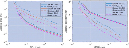
Figure 6. Error convergence for the price (left) and the optimal exercise boundary (right) with respect to CPU time; the underlying asset is modelled with a Gaussian process and the risk-free rate is r = 0.05. The pricing error convergence of the new method described in section 4.2 and labelled ‘Spitzer’ is faster than that of the residue method described in section 4.1 and labelled ‘Green’, whereas the optimal exercise boundary error convergence is worse.

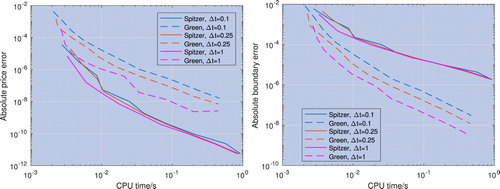
Table 2. Results for both methods for perpetual Bermudan options with $2^{20}$ log-price grid points showing the convergence to the price for a perpetual American option.

	Spitzer			Green
$\mathrm{\Delta }t$	r = 0.1	r = 0.05	r = 0.02	r = 0.1	r = 0.05	r = 0.02
1	0.20169919	0.33181098	0.53155442	0.20169919	0.33181098	0.53155362
0.5	0.20737414	0.33522271	0.53328533	0.20737414	0.33522271	0.53328453
0.25	0.21021533	0.33695115	0.53414348	0.21021533	0.33695115	0.53414268
0.1	0.21197983	0.33798846	0.53465453	0.21197984	0.33798846	0.53465373
0.01	0.21305064	0.33861012	0.53495870	0.21305065	0.33861013	0.53495791
American	0.21317038	0.33867902	0.53499224	0.21317038	0.33867902	0.53499224

Table 3. Optimal exercise boundary calculated using both methods for perpetual Bermudan options with $2^{20}$ log-price grid points showing the convergence to the optimal exercise boundary for a perpetual American option.

	Spitzer			Green
$\mathrm{\Delta }t$	r = 0.1	r = 0.05	r = 0.02	r = 0.1	r = 0.05	r = 0.02
1	0.68360194	0.47916587	0.25110359	0.68360124	0.47916517	0.25110066
0.5	0.64678075	0.45056945	0.23520061	0.64678008	0.45056880	0.23519670
0.25	0.62026498	0.43075700	0.22442626	0.62026434	0.43075637	0.22442094
0.1	0.59653531	0.41350275	0.21519240	0.59653469	0.41350214	0.21518427
0.01	0.56851217	0.39363474	0.20472988	0.56851159	0.39363417	0.20470522
American	0.55555556	0.38461538	0.20000000	0.55555556	0.38461538	0.20000000

Both methods perform well, and as $\mathrm{\Delta }t\to 0$ the results approach those for the corresponding perpetual American option. The new Spitzer-based method outperforms Green's residue method, achieving an error of ${10}^{-7}$ in approximately one tenth of the CPU time. In contrast, the convergence of the optimal exercise boundary is slower for the Spitzer-based method than for Green's residue method. Moreover the optimal exercise boundary errors of both methods converge at the same rate or slower than the price errors, so we can see that the former has a limited effect on the latter. This is discussed in more detail in section 4.4.1.

4.4.1. Effect of the optimal exercise boundary error

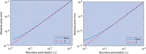
We studied the effect of the optimal exercise boundary error in more detail by adding a perturbation (i.e. a small additional error) to the optimal exercise boundary and observing the effect on the absolute error of the price. Figure 7 shows the result of this for log-price grid sizes of $2^{18}$ and $2^{21}$ which in the original results correspond to price errors of 1.9E−9 and 2.1E−12 respectively and exercise boundary errors of 1.4E−5 and 8.7E−7, respectively. We can clearly see that there is a quadratic relationship between the error of the optimal exercise boundary and the error of the price. This is consistent with the fact that the price error caused by the boundary error is equal to the area between the lines of the payoff $K-S_0$ and the intrinsic option value $v(0,0)$ in figure 4.

Figure 7. The absolute price error for different levels of perturbation added to the optimal exercise boundary for log-price grid sizes of $2^{18}$ (left) and $2^{21}$ (right). The smallest perturbation is equal to the boundary error at the same grid size, i.e. the smallest error result has twice the boundary error usually seen. Notice the quadratic relationship between boundary error and absolute error.

4.5. Results for perpetual Bermudan options with other Lévy processes

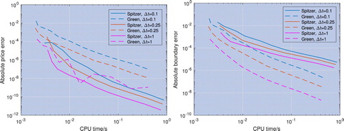
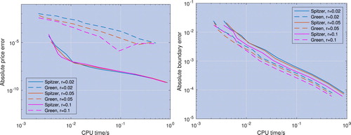
Figures 8–11 show results for the price and optimal exercise boundary error vs. the number of grid points and CPU time, with the log-price of the underlying asset modelled by VG and Merton processes. Once again, the Spitzer-based method performs better, achieving an error of ${10}^{-7}$ about 10 times quicker than Green's method. The error is calculated as the precision compared to the result with the maximum number of grid points and we discuss the verification of these results below.

Figure 8. Error convergence for the price (left) and the optimal exercise boundary (right) with respect to CPU time; the underlying asset is modelled with a VG process and the risk-free rate is r = 0.02. The pricing error convergence of the new method described in section 4.2 and labelled ‘Spitzer’ is faster than that of the residue method described in section 4.1 and labelled ‘Green’, whereas the optimal exercise boundary error convergence is worse.

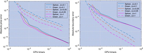
Figure 9. Error convergence for the price (left) and the optimal exercise boundary (right) with respect to CPU time; the underlying asset is modelled with a VG process and the risk-free rate is r = 0.05. The pricing error convergence of the new method described in section 4.2 and labelled ‘Spitzer’ is faster than that of the residue method described in section 4.1 and labelled ‘Green’, whereas the optimal exercise boundary error convergence is worse.

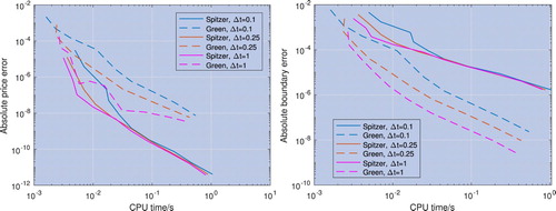
Figure 10. Error convergence for the price (left) and the optimal exercise boundary (right) with respect to CPU time; the underlying asset is modelled with a Merton jump-diffusion process and the risk-free rate is r = 0.02. The pricing error convergence of the new method described in section 4.2 and labelled ‘Spitzer’ is faster than that of the residue method described in section 4.1 and labelled ‘Green’, whereas the optimal exercise boundary error convergence is worse.

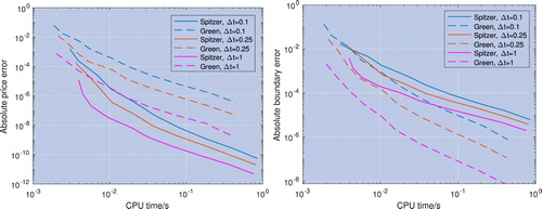
Figure 11. Error convergence for the price (left) and the optimal exercise boundary (right) with respect to CPU time; the underlying asset is modelled with a Merton jump-diffusion process and the risk-free rate is r = 0.05. The pricing error convergence of the new method described in section 4.2 and labelled ‘Spitzer’ is faster than that of the residue method described in section 4.1 and labelled ‘Green’, whereas the optimal exercise boundary error convergence is worse.

In tables 2 and 3 we showed that that the results with the Gaussian process converge to the closed-form solution by Merton (1973) as $\mathrm{\Delta }t\to 0$. We do not have a closed-form solution for other Lévy processes, so we computed Monte Carlo estimates for the Gaussian, VG and Merton cases.

Although the discrete nature of perpetual Bermudan options is appropriate for a Monte Carlo simulation, the absence of an expiry means that a Monte Carlo scheme with a finite number of dates will not be a true representation of the contract. We truncate the Monte Carlo simulation far enough in the future that the effect of disregarding these future dates is less than the standard deviation of the Monte Carlo method itself (clearly this method is more feasible for high discount factors and large monitoring intervals, as the effect of future dates is discounted away more rapidly). The calculation of the optimal exercise boundary uses the same approach as the new method described in section 4.2, i.e. we calculated the price for $S_0=D_1$ and $S_0=D_2$, then we found the intersection between the line through these points and the non-zero part of the payoff function $(K-S_0{)}^{+}$, i.e. $K-S_0$ for $S_0<K$.

Table 4 shows that for all tested cases the results of our new methods described in sections 4.1 and 4.2 coincide and are within 2 standard deviations from the Monte Carlo results, i.e. within a confidence interval of about 95%. More details about this Monte Carlo scheme are included in Appendix 3.

Table 4. Comparison between the value of a perpetual Bermudan option with $2^{20}$ log-price grid points and the value for the same contract using a Monte Carlo approximation.

Parameters		Monte Carlo
r	$\mathrm{\Delta }t$	price	std dev	Spitzer price	Green price
Gaussian
0.05	1	0.33180	4.2E−5	0.331811	0.331811
0.05	0.5	0.33520	4.5E−5	0.335223	0.335223
0.05	0.25	0.33695	4.5E−5	0.336951	0.336951
0.05	0.1	0.33791	8.3E−5	0.337988	0.337988
Variance gamma
0.05	1	0.12023	1.1E−4	0.120237	0.120237
0.05	0.5	0.12342	2.3E−4	0.123298	0.123298
0.05	0.25	0.12500	1.3E−4	0.124919	0.124919
0.05	0.1	0.12588	1.3E−4	0.125959	0.125959
0.02	1	0.24704	1.8E−4	0.247078	0.247078
0.02	0.1	0.24975	1.8E−4	0.249756	0.249756
Merton jump-diffusion
0.05	1	0.11976	1.3E−4	0.119856	0.119856
0.05	0.5	0.12309	1.2E−4	0.122993	0.122993
0.05	0.25	0.12464	1.4E−4	0.124674	0.124674
0.05	0.1	0.12570	1.1E−4	0.125767	0.125767

Note: The prices calculated using the new Spitzer-based method and Green's method are the same and within two standard deviations of the Monte Carlo price.

5. Perpetual American options

As described by Green et al. (2010) and implemented by Phelan et al. (2018), we can exploit the relationship between Laplace and z-transforms described in equation (9(9) ${\mathcal{L}}_{t\to s}\left[f\right(t\left)\right]=\underset{\mathrm{\Delta }t\to 0}{lim}\mathrm{\Delta }t{\mathcal{Z}}_{n\to q}\left[f\right(t_n\left)\right].$(9) ) to extend the pricing methods from discrete to continuous monitoring, in this case from perpetual Bermudan to perpetual American options. Unlike the previous examples for option pricing with continuous monitoring, where the application of option pricing was used as a motivating example for techniques which have relevance in other fields, the continuous (i.e. American) case is commonly used in financial contracts. By defining $q={\mathrm{e}}^{-s\mathrm{\Delta }t}$, we can write the continuously monitored equivalent to $\mathrm{\Phi }(\xi ,q)=1-q\mathrm{\Psi }(\xi ,\mathrm{\Delta }t)$ as ${\mathrm{\Phi }}_{\mathrm{c}}(\xi ,s)=s-\psi \left(\xi \right)$, where $\psi \left(\xi \right)$ is the characteristic exponent of the characteristic function $\mathrm{\Psi }(\xi ,\mathrm{\Delta }t)$. Here, as $q={\mathrm{e}}^{-r\mathrm{\Delta }t}$, we have s = r. Both methods described in sections 4.1 and 4.2 can be converted to continuous monitoring and we compare the results below.

5.1. Results for perpetual American options

Figures 12–14 show results for both methods with the Gaussian, VG and Merton processes. To assess the accuracy of the methods with a Gaussian process we have the advantage over Bermudan options that closed-form formulas exist for the calculation of both the optimal exercise boundary and the option price, and so the results in figure 12 use the closed-form calculation from Merton (1973) to calculate the error. For the other process we do not have a closed-form result, and the continuous nature of American options means that they cannot be accurately represented using Monte Carlo methods which are inherently discrete. Therefore the absolute errors displayed in figures 13 and 14 are calculated against the result for the same method and process with the maximum number of log-price grid points.

Figure 12. Error convergence for the price (left) and the optimal exercise boundary (right) with respect to CPU time; the log-price of the underlying asset is modelled by a Gaussian process with a range of risk-free rates r. The error is calculated using the closed-form expression by Merton as a reference. The price and optimal exercise boundary error convergence for the new method described in section 4.2 labelled ‘Spitzer’ is faster than for the residue method described in section 4.1 labelled ‘Green’.

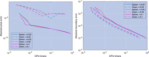
Figure 13. Error convergence for the price (left) and the optimal exercise boundary (right) with respect to CPU time; the log-price of the underlying asset is modelled by a VG process with a range of risk-free rates r. The error is calculated using the numerical result with the maximum grid size as a reference. The price and optimal exercise boundary error convergence for the new method described in section 4.2 labelled ‘Spitzer’ is faster than for the residue method described in section 4.1 labelled ‘Green’.

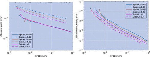
Figure 14. Error convergence for the price (left) and the optimal exercise boundary (right) with respect to CPU time; the log-price of the underlying asset is modelled by a Merton jump-diffusion process with a range of risk-free rates r. The error is calculated using the numerical result with the maximum grid size as a reference. The price and optimal exercise boundary error convergence for the new method described in section 4.2 labelled ‘Spitzer’ is faster than for the residue method described in section 4.1 labelled ‘Green’.

In contrast to the results for perpetual Bermudan options, the performance of the two methods is very different. Our new Spitzer-based method is far superior, giving errors of approximately ${10}^{-6}$ in ${10}^{-2}$ seconds or less. For the Gaussian and Merton processes, Green's method fails to reach an error level of ${10}^{-6}$, and for the VG process it reaches this level about 100 times slower than our new method.

5.2. Comparison between American and Bermudan option prices

The performance for the direct calculation of the price of American options is sufficiently good for practical purposes, with the Spitzer method having an error of ${10}^{-6}$ for a CPU time of ${10}^{-2}$ s. However, it is of academic interest to study the use of the price for Bermudan options as an approximation to the price for American options.

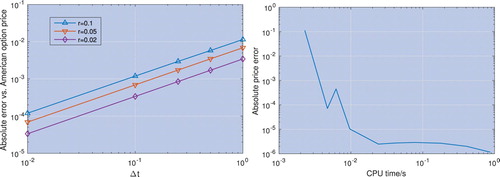
The left-hand panel in figure 15 shows the price error compared to American options plotted against $\mathrm{\Delta }t$ with the log-price of the underlying asset modelled by a Gaussian process and it is clear that the relationship is linear. By extrapolating this line, we can see that in order to achieve an error of ${10}^{-8}$ for r = 0.02 a step size of $\mathrm{\Delta }t=0.3$E−06 is required. The price convergence with this step size is shown in figure 15 and we can see that reducing the step size this low destroys the monotonicity of the convergence and the excellent error performance that we were seeing for more realistic step sizes.

Figure 15. Convergence of the price of perpetual Bermudan options to the price of perpetual American options. The left hand plot shows the convergence as $\mathrm{\Delta }t\to 0$ with the log-price of the underlying asset modelled by a Gaussian process. The right hand side plot shows the error convergence of the price of a perpetual Bermudan option with r = 0.02 and $\mathrm{\Delta }t=$3E−06 vs. CPU time.

6. Conclusion

We implemented three new pricing methods based on the Spitzer identities for pricing exotic options. We saw very fast error convergence with log-price grid size and, by extension, CPU time. Due to the low errors and the presence of the ${10}^{-11}$ error floor in the inverse z-transform, it was not possible to identify whether the error convergence is exponential or high-order polynomial. The extremely low error and computational time make this a highly attractive method as it stands. However, it would be of academic interest to implement this method using an inverse z-transform with a lower error floor in order to determine the exact order of convergence.

We presented a novel method for pricing perpetual Bermudan options which includes a new technique to directly compute the optimal exercise boundary; it is based on the Spitzer identities and the sinc-based fast Hilbert transform. We also provide the first numerical implementation of a method designed by Green (2009) which uses residue calculus to remove the requirement of the final inverse Fourier-z transform. Both methods perform well, but our new method shows significantly lower errors and CPU times, with a computational speed ten times faster for an error of ${10}^{-7}$.

We extended these methods to perpetual American options (i.e. with continuous monitoring) and very different results were observed for the two methods. For Green's method, the factorisation error was very high and dominated the error convergence. For the new Spitzer-based method, the factorisation error was much lower and therefore the effect only became dominant for errors below approximately ${10}^{-7}$.

For errors greater than ${10}^{-7}$, the new Spitzer-based method for perpetual American options has errors at least as low as the method for perpetual Bermudan options, so we conclude that, for practical purposes, there is no advantage in using discrete monitoring as an approximation for continuous monitoring. Comparing the two approaches as an academic exercise shows that there is as a linear relationship between the size of the monitoring interval $\mathrm{\Delta }t$ and the error compared to continuous monitoring. However, reducing $\mathrm{\Delta }t$ to a sufficiently low value that the discrete method would be predicted to have a lower error than the continuous method, significantly degrades the error convergence of the discretely monitored method so that no advantage is gained.

An interesting extension to this work would be to investigate the calculation of the Greeks for these options. Several different approaches have been used in the literature to find the Greeks with Fourier-based methods. These include analytic methods such as those by Olivera and Mordecki (2016), Eberlein et al. (2010) and Takahashi and Yamazaki (2009), based on the work by Carr and Madan (1999) and Lewis (2001). In addition, numerical methods have been developed for path-dependent options, such as those by Jeannin and Pistorius (2009).

Disclosure statement

No potential conflict of interest was reported by the authors.

ORCID

C. E. Phelan http://orcid.org/0000-0001-6500-6954

D. Marazzina http://orcid.org/0000-0001-6107-9822

G. Germano http://orcid.org/0000-0003-4441-9842

Additional information

Funding

The support of the Economic and Social Research Council (ESRC) in funding the Systemic Risk Centre [grant number ES/K002309/1] and of the Engineering and Physical Sciences Research Council (EPSRC) in funding the UK Centre for Doctoral Training in Financial Computing and Analytics [grant number EP/L015129/1] are gratefully acknowledged.

Notes

1 See section 2 for a discussion of the purpose of the damping factor and the choice of the damping paramter.

Appendix 1. Numerical pricing procedures

Detailed descriptions of the pricing schemes are given in Sections 3–5 of the main paper. Here we also provide detailed step-by-step procedures used for our MATLAB implementation.

A.1. Green's residue method for perpetual Bermudan options

1. Compute the characteristic function $\mathrm{\Psi }(\xi +i{\alpha }_{\mathrm{d}})$, where ${\alpha }_{\mathrm{d}}$ is the damping parameter.

2. Use the Plemelj–Sokhotsky relations with the sinc-based fast Hilbert transform to factorise (A1) $\begin{array}{rl}\mathrm{\Phi }(\xi ,q)& :=1-{\mathrm{e}}^{-r\mathrm{\Delta }t}\sigma \left(\xi /{\xi }_{max}\right)\mathrm{\Psi }(\xi +i{\alpha }_{\mathrm{d}},\mathrm{\Delta }t)\\ & ={\mathrm{\Phi }}_{\oplus }(\xi ,{\mathrm{e}}^{-r\mathrm{\Delta }t}){\mathrm{\Phi }}_{\ominus }(\xi ,{\mathrm{e}}^{-r\mathrm{\Delta }t}),\end{array}$(A1) where $\sigma \left(\eta \right)$ is an exponential filter of order 12 (Gottlieb and Shu 1997). From this we can directly obtain ${\mathrm{\Phi }}_{\ominus }(0,{\mathrm{e}}^{-r\mathrm{\Delta }t})$.

3. Use the shift theorem to calculate ${\mathrm{\Phi }}_{\ominus }(i,{\mathrm{e}}^{-r\mathrm{\Delta }t})$ as (A2) $\begin{array}{r}{\mathrm{\Phi }}_{\ominus }(i,{\mathrm{e}}^{-r\mathrm{\Delta }t})={\mathcal{F}}_{x\to \xi }\left[{\mathrm{e}}^{-x}{\mathcal{F}}_{\xi \to x}^{-1}\left[{\mathrm{\Phi }}_{\ominus }(\xi ,{\mathrm{e}}^{-r\mathrm{\Delta }t})\right]\right]\left(0\right).\end{array}$(A2)

4. Calculate the optimal exercise boundary (A3) $D_{\mathrm{o}\mathrm{p}\mathrm{t}}=K\frac{{\mathrm{\Phi }}_{\ominus }(0,{\mathrm{e}}^{-r\mathrm{\Delta }t})}{{\mathrm{\Phi }}_{\ominus }(i,{\mathrm{e}}^{-r\mathrm{\Delta }t})}$(A3) and the log-boundary $l_{\mathrm{o}\mathrm{p}\mathrm{t}}=\log \left(D_{\mathrm{o}\mathrm{p}\mathrm{t}}/S_0\right)$.

5. Decompose $P(\xi ,{\mathrm{e}}^{-r\mathrm{\Delta }t})=1/{\mathrm{\Phi }}_{\ominus }(0,{\mathrm{e}}^{-r\mathrm{\Delta }t})$ around $l_{\mathrm{o}\mathrm{p}\mathrm{t}}$, (A4) $P(\xi ,{\mathrm{e}}^{-r\mathrm{\Delta }t})=P_{l_{\mathrm{o}\mathrm{p}\mathrm{t}}+}(\xi ,{\mathrm{e}}^{-r\mathrm{\Delta }t})+P_{l_{\mathrm{o}\mathrm{p}\mathrm{t}}-}(\xi ,{\mathrm{e}}^{-r\mathrm{\Delta }t})$(A4) and obtain $P_{l_{\mathrm{o}\mathrm{p}\mathrm{t}}-}(0,{\mathrm{e}}^{-r\mathrm{\Delta }t})$.

6. Use the shift theorem to calculate (A5) $\begin{array}{r}{P}_{l_{\mathrm{o}\mathrm{p}\mathrm{t}}-}(i,{\mathrm{e}}^{-r\mathrm{\Delta }t}):={\mathcal{F}}_{\xi \to \xi }\left[{\mathrm{e}}^{-x}{\mathcal{F}}_{\xi \to x}^{-1}\left[P_{l_{\mathrm{o}\mathrm{p}\mathrm{t}}-}(0,{\mathrm{e}}^{-r\mathrm{\Delta }t})\right]\right]\left(0\right).\end{array}$(A5)

7. Calculate the option price (A6) $\begin{array}{rl}v(0,0)& =K{\mathrm{\Phi }}_{\ominus }(0,{\mathrm{e}}^{-r\mathrm{\Delta }t})\\ & \times \left[P_{l_{\mathrm{o}\mathrm{p}\mathrm{t}}-}(0,{\mathrm{e}}^{-r\mathrm{\Delta }t})-P_{l_{\mathrm{o}\mathrm{p}\mathrm{t}}-}(i,{\mathrm{e}}^{-r\mathrm{\Delta }t})\right].\end{array}$(A6)

A.2. Spitzer-based method for perpetual Bermudan options

1. Compute the characteristic function $\mathrm{\Psi }(\xi +i{\alpha }_{\mathrm{d}})$, where ${\alpha }_{\mathrm{d}}$ is the damping parameter.

2. Use the Plemelj–Sokhotsky relations with the sinc-based fast Hilbert transform to factorise (A7) $\begin{array}{rl}\mathrm{\Phi }(\xi ,q)& :=1-{\mathrm{e}}^{-r\mathrm{\Delta }t}\sigma \left(\xi /{\xi }_{max}\right)\mathrm{\Psi }(\xi +i{\alpha }_{\mathrm{d}},\mathrm{\Delta }t)\\ & ={\mathrm{\Phi }}_{\oplus }(\xi ,{\mathrm{e}}^{-r\mathrm{\Delta }t}){\mathrm{\Phi }}_{\ominus }(\xi ,{\mathrm{e}}^{-r\mathrm{\Delta }t}),\end{array}$(A7) where $\sigma \left(\eta \right)$ is an exponential filter of order 12.

3. Decompose $P(\xi ,{\mathrm{e}}^{-r\mathrm{\Delta }t})=1/{\mathrm{\Phi }}_{\oplus }(\xi ,{\mathrm{e}}^{-r\mathrm{\Delta }t})$ around the log-price grid step $l_{ϵ}=\mathrm{\Delta }x$, (A8) $P(\xi ,{\mathrm{e}}^{-r\mathrm{\Delta }t})=P_{l_{ϵ}+}(\xi ,{\mathrm{e}}^{-r\mathrm{\Delta }t})+P_{l_{ϵ}-}(\xi ,{\mathrm{e}}^{-r\mathrm{\Delta }t}).$(A8)

4. Calculate the PDF for the calibration (A9) ${\hat{p}}_{l_{ϵ}-}(\xi ,{\mathrm{e}}^{-r\mathrm{\Delta }t})=P_{l_{ϵ}-}(\xi ,{\mathrm{e}}^{-r\mathrm{\Delta }t}){\mathrm{\Phi }}_{\ominus }(\xi ,{\mathrm{e}}^{-r\mathrm{\Delta }t}).$(A9)

5. Setting $D_1$ = 0 and $D_2\in (0,K)$, calculate (A10) $\begin{array}{rl}{v}_{{\mathrm{D}}_1}(0,0)& =K{\hat{p}}_{l_{ϵ}-}(0,{\mathrm{e}}^{-r\mathrm{\Delta }t})\end{array}$(A10) (A11) $\begin{array}{rl}{v}_{{\mathrm{D}}_2}(0,0)& ={\mathcal{F}}_{\xi \to x}^{-1}[{\hat{\phi }}^{\ast }\left(\xi \right){\hat{p}}_{l_{ϵ}-}(0,{\mathrm{e}}^{-r\mathrm{\Delta }t})]\left(0\right),\end{array}$(A11) where $\hat{\phi }\left(\xi \right)$ is the Fourier transform of the damped payoff $\phi \left(x\right)$ with $x=\log \left(S\right(t\left)/D_2\right)$.

6. Calculate the optimal exercise boundary (A12) $D_{\mathrm{o}\mathrm{p}\mathrm{t}}=\frac{\left[K-v_{{\mathrm{D}}_1}(0,0)\right]D_2}{v_{{\mathrm{D}}_2}(0,0)-v_{{\mathrm{D}}_1}(0,0)+D_2}$(A12) and the log-boundary $l_{\mathrm{o}\mathrm{p}\mathrm{t}}=\log \left(D_{\mathrm{o}\mathrm{p}\mathrm{t}}/S_0\right)$.

7. Decompose $P(\xi ,{\mathrm{e}}^{-r\mathrm{\Delta }t})=1/{\mathrm{\Phi }}_{\oplus }(\xi ,{\mathrm{e}}^{-r\mathrm{\Delta }t})$ around $l_{\mathrm{o}\mathrm{p}\mathrm{t}}$, (A13) $P(\xi ,{\mathrm{e}}^{-r\mathrm{\Delta }t})=P_{l_{\mathrm{o}\mathrm{p}\mathrm{t}}+}(\xi ,{\mathrm{e}}^{-r\mathrm{\Delta }t})+P_{l_{\mathrm{o}\mathrm{p}\mathrm{t}}-}(\xi ,{\mathrm{e}}^{-r\mathrm{\Delta }t}).$(A13)

8. Calculate the characteristic function of the log-price (A14) ${\hat{p}}_{l_{\mathrm{o}\mathrm{p}\mathrm{t}}}(\xi ,{\mathrm{e}}^{-r\mathrm{\Delta }t})=P_{l_{\mathrm{o}\mathrm{p}\mathrm{t}}-}(\xi ,{\mathrm{e}}^{-r\mathrm{\Delta }t}){\mathrm{\Phi }}_{\ominus }(\xi ,{\mathrm{e}}^{-r\mathrm{\Delta }t}).$(A14)

9. Calculate the option price (A15) $v(0,0)={\mathcal{F}}_{\xi \to x}^{-1}[{\hat{\phi }}^{\ast }\left(\xi \right){\hat{p}}_{l_{\mathrm{o}\mathrm{p}\mathrm{t}}}(0,{\mathrm{e}}^{-r\mathrm{\Delta }t})]\left(0\right),$(A15) where $\hat{\phi }\left(\xi \right)$ is the Fourier transform of the damped payoff $\phi \left(x\right)$ with $x=\log \left(S\right(t\left)/S_0\right)$.

A.3. Perpetual American options

For both methods the pricing procedure for discretely monitored options is adapted to continuous monitoring by replacing Steps (i)–(ii) in sections A.1 and A.2 with

1. Compute the characteristic exponent $\psi (\xi +i{\alpha }_{\mathrm{d}})$ of the underlying transition density.

2. Use the Plemelj–Sokhotsky relations, equations (11(11) $\begin{array}{rl}\widehat{f_{l+}}\left(\xi \right)& =\frac{1}{2}\{\hat{f}\left(\xi \right)+e^{il\xi }i\mathcal{H}[{\mathrm{e}}^{-il\xi }\hat{f}\left(\xi \right)]\}\end{array}$(11) )–(12(12) $\begin{array}{rl}\widehat{f_{l-}}\left(\xi \right)& =\frac{1}{2}\{\hat{f}\left(\xi \right)-e^{il\xi }i\mathcal{H}[{\mathrm{e}}^{-il\xi }\hat{f}\left(\xi \right)]\}.\end{array}$(12) ), with the sinc-based fast Hilbert transform to factorise (A16) ${\mathrm{\Phi }}_{\mathrm{c}}(\xi ,r):=r-\psi (\xi +i{\alpha }_{\mathrm{d}})={\mathrm{\Phi }}_{\mathrm{c}\oplus }(\xi ,r){\mathrm{\Phi }}_{\mathrm{c}\ominus }(\xi ,r),$(A16) where r is the risk-free rate.

Then continue with Step (iii) in sections A.1 or A.2, but with ${\mathrm{\Phi }}_{\mathrm{c}}(\xi ,r)$ in place of $\mathrm{\Phi }(\xi ,{\mathrm{e}}^{-r\mathrm{\Delta }t})$.

Appendix 2. Process parameters

Table 5 contains the process parameters used for the numerical tests.

Table A1. Parameters for the numerical tests; $\mathrm{\Psi }(\xi ,t)$ is the characteristic function of the process that models the log-price of the underlying asset.

Process	$\mathrm{\Psi }(\xi ,t)$	Symbol	Value
Gaussian	$e^{(i\mu \xi -(1/2\left){\sigma }^2{\xi }^2\right)t}$	μ	0
		σ	0.4
Variance gamma	$(1-i\nu \xi \theta +\frac{1}{2}\nu {\sigma }^2{\xi }^2{)}^{-t/\nu }$	θ	$\frac{1}{9}$
		σ	$\frac{1}{3\sqrt{3}}$
		ν	0.25
Merton jump-diffusion	$e^{(-(1/2){\sigma }^2{\xi }^2+\lambda (e^{i{\mu }_{\mathrm{J}}\xi -\left(1/2\right){\sigma }_{\mathrm{J}}^2{\xi }^2}-1\left)\right)t}$	σ	0.1
		λ	3
		${\mu }_J$	−0.05
		${\sigma }_J$	0.086

Appendix 3. Monte Carlo pricing procedures

We describe in detail the Monte Carlo procedures which we used to validate the prices calculated by the numerical methods presented in this paper.

A.4. Path generation

For underlying assets with log-prices modelled by Gaussian, variance gamma and Merton processes $X\left(t\right)$, the paths can simply be constructed using the Euler–Maruyama algorithm with the built-in Matlab functions for normal, gamma and Poisson pseudo-random variables (Ballotta and Fusai 2018). In all cases the risk-neutral drift was calculated using ${\mu }_{\mathrm{R}\mathrm{N}}=\psi (-i)$ as described by Feng and Linetsky (2008), where $\psi \left(\xi \right)$ is the characteristic exponent of the Lévy process.

A step of the Gaussian process (arithmetic Brownian motion) was simulated with (A17) $\mathrm{\Delta }X={\mu }_{\mathrm{R}\mathrm{N}}\mathrm{\Delta }t+\sigma \sqrt{\mathrm{\Delta }t}Z,$(A17) where $Z\stackrel{d}{=}N(0,1)$ is a standard normal random variable.

A step of the variance gamma (VG) process was simulated with (A18) $\mathrm{\Delta }X={\mu }_{\mathrm{R}\mathrm{N}}\mathrm{\Delta }t+\theta G+\sigma \sqrt{G}Z,$(A18) where $G\stackrel{d}{=}\mathrm{\Gamma }\left(1/\right(\nu \mathrm{\Delta }t),\nu )$ is a gamma-distributed random variable and Z is a standard normal random variable.

A step of the Merton jump-diffusion (MJD) process was simulated with (A19) $\mathrm{\Delta }X={\mu }_{\mathrm{R}\mathrm{N}}\mathrm{\Delta }t+\sigma \sqrt{\mathrm{\Delta }t}{Z}_1+{\mu }_{\mathrm{J}}Y+{\sigma }_{\mathrm{J}}\sqrt{Y}{Z}_2,$(A19) where $Y\stackrel{d}{=}\mathrm{P}\mathrm{o}\mathrm{i}\left(\lambda \mathrm{\Delta }t\right)$ is a Poisson-distributed random variable and $Z_1$ and $Z_2$ are independent standard normal random variables.

A.5. α-quantile options

We used two methods to calculate the α-quantile:

1. We simulated a path of N points and then found the jth smallest value, where $j=\alpha N$ rounded to the nearest integer.

2. We combined Monte Carlo with the Dassios–Port–Wendel identity as in Ballotta and Kyprianou (2001): two independent paths over j and N−j dates are simulated and the sum of their respective maximum and minimum is taken to provide an estimate of the α-quantile.

A.6. Perpetual Bermudan options

Although the discrete nature of perpetual Bermudan options is appropriate for a Monte Carlo simulation, the absence of an expiry means that a Monte Carlo scheme with a finite number of dates will not represent the contract exactly. However, we truncate the Monte Carlo simulation so far in the future that the effect of disregarding these dates is less than the standard deviation of the Monte Carlo method itself; this value has been determined empirically. Clearly this is more accurate for high discount factors and large monitoring intervals because the effect of future dates is discounted away more rapidly. The optimal exercise boundary is found with the same approach as in the new method described in section 4.2: the price is calculated for $S_0=D_1$ and $S_0=D_2$, then the boundary is taken as the intersection between the line through these points and the non-zero part of the payoff function $(K-S_0{)}^{+}$, i.e. the line $K-S_0$ for $S_0<K$.

References

- Abate, J. and Whitt, W., Numerical inversion of probability generating functions. Oper Res. Lett., 1992, 12(4), 245–251.
- Abate, J. and Whitt, W., Numerical inversion of Laplace transforms of probability distributions. ORSA J. Comput., 1995, 7(1), 36–43.
- Akahori, J., Some formulae for a new type of path-dependent option. Ann. Appl. Probab., 1995, 5(2), 383–388.
- Atkinson, C. and Fusai, G., Discrete extrema of Brownian motion and pricing of exotic options. J. Comput. Finance, 2007, 10(3), 1–43.
- Ballotta, L., α-quantile option in a jump-diffusion economy. In Financial Engineering, E-commerce and Supply Chain, edited by P.M. Pardalos and V.K. Tsitsiringos, pp. 75–87, 2002 (Springer: Boston, MA).
- Ballotta, L. and Fusai, G., Tools from Stochastic Analysis for Mathematical Finance: A Gentle Introduction, SSRN 3183712, 2018.
- Ballotta, L. and Kyprianou, A.E., A note on the α-quantile option. Appl. Math. Financ., 2001, 8(3), 137–144.
- Barone-Adesi, G., The saga of the American put. J. Bank. Financ., 2005, 29, 2909–2918.
- Battauz, A., Donno, M.D. and Sbuelz, A., Real options and American derivatives: The double continuation region. Manage. Sci., 2015, 61, 1094–1107.
- Baxter, G. and Donsker, M.D., On the distribution of the supremum functional for processes with stationary independent increments. Trans. Am. Math. Soc., 1957, 85(1), 73–87.
- Borovkov, K. and Novikov, A., On a new approach to calculating expectations for option pricing. J. Appl. Probab., 2002, 39, 889–895.
- Boyarchenko, S.I. and Levendorskii, S.Z., Perpetual American options under Lévy processes. SIAM J. Control Optim., 2002a, 40(6), 1663–1696.
- Boyarchenko, S.I. and Levendorskii, S.Z., Pricing of perpetual Bermudan options. Quant. Finance, 2002b, 2(6), 432–442.
- Boyd, J.P., Chebyshev and Fourier Spectral Methods, 2001 (Springer: Heidelberg).
- Brennan, M.J. and Schwartz, E.S., The valuation of American put options. J. Financ., 1977, 32(2), 449–462.
- Broadie, M., Glasserman, P. and Kou, S., A continuity correction for discrete barrier options. Math. Financ., 1997, 7(4), 325–349.
- Cai, N., Chen, N. and Wan, X., Occupation times of jump-diffusion processes with double exponential jumps and the pricing of options. Math. Oper. Res., 2010, 35(2), 412–437.
- Carr, P. and Madan, D., Option valuation using the fast Fourier transform. J. Comput. Financ., 1999, 2, 61–73.
- Cox, J.C., Ross, S.A. and Rubinstein, M., Option pricing: A simplified approach. J. Financ. Econ., 1979, 7(3), 229–263.
- Cui, Z., Kirkby, J.L. and Nguyen, D., Equity-linked annuity pricing with cliquet-style guarantees in regime-switching and stochastic volatility models with jumps. Insur.: Math. Econ., 2017, 74, 46–62.
- Darling, D.A., Liggett, T. and Taylor, H.M., Optimal stopping for partial sums. Ann. Math. Stat., 1972, 43(4), 1363–1368.
- Dassios, A., The distribution of the quantile of a Brownian motion with drift and the pricing of related path-dependent options. Ann. Appl. Probab., 1995, 5(2), 389–398.
- Dassios, A., Quantiles of Lévy processes and applications in finance. Working paper, Department of Statistics, London School of Economics and Political Science, 2006.
- Du, D. and Luo, D., The pricing of jump propagation: Evidence from spot and options markets. Manage. Sci., 2019, 65, 1949–2443.
- Eberlein, E., Glau, K. and Papapantoleon, A., Analysis of Fourier transform valuation formulas and applications. Appl. Math. Financ., 2010, 17, 211–240.
- Eberlein, E., Glau, K. and Papapantoleon, A., Analyticity of the Wiener–Hopf factors and valuation of exotic options in Lévy models. In Advanced Mathematical Methods for Finance, edited by G.D. Nunno and B. Øksendal, pp. 223–245, 2011 (Springer: Berlin).
- Feng, L. and Lin, X., Pricing Bermudan options in Lévy process models. SIAM J. Financ. Math., 2013, 4(1), 474–493.
- Feng, L. and Linetsky, V., Pricing discretely monitored barrier options and defaultable bonds in Lévy process models: A Hilbert transform approach. Math. Financ., 2008, 18(3), 337–384.
- Feng, L. and Linetsky, V., Computing exponential moments of the discrete maximum of a Lévy process and lookback options. Financ. Stoch., 2009, 13, 501–529.
- Fusai, G., Abrahams, I.D. and Sgarra, C., An exact analytical solution for discrete barrier options. Financ. Stoch., 2006, 10(1), 1–26.
- Fusai, G., Germano, G. and Marazzina, D., Spitzer identity, Wiener–Hopf factorisation and pricing of discretely monitored exotic options. Eur. J. Oper. Res., 2016, 251, 124–134.
- Fusai, G. and Tagliani, A., Pricing of occupation time derivatives: Continuous and discrete monitoring. J. Comput. Finance, 2001, 5(1), 1–38.
- Gottlieb, D. and Shu, C., On the Gibbs phenomenon and its resolution. SIAM Rev., 1997, 39(4), 644–668.
- Green, R., Application of the Wiener-Hopf technique to derivative pricing. PhD Thesis, University of Manchester, 2009.
- Green, R., Fusai, G. and Abrahams, I.D., The Wiener-Hopf technique and discretely monitored path-dependent option pricing. Math. Finance, 2010, 20(2), 259–288.
- Haslip, G.G. and Kaishev, V.K., Lookback option pricing using the Fourier transform B-spline method. Quant. Finance, 2014, 14, 789–803.
- Jeannin, M. and Pistorius, M., A transform approach to compute prices and greeks of barrier options driven by a class of Lévy processes. Quant. Finance, 2009, 10, 629–644.
- Kahl, C. and Lord, R., Fourier inversion methods in finance. In Handbook of Computational Finance, 2010. Available online at: http://www.rogerlord.com/fourierinversionmethods.pdf.
- Kou, S., A jump-diffusion model for option pricing. Manage. Sci., 2002, 48, 1086–1101.
- Kreyszig, E., Advanced Engineering Mathematics, 10th edition, 2011 (Wiley: New York).
- Lewis, A.L., A simple option formula for general jump-diffusion and other exponential Lévy processes, 2001. doi:10.2139/ssrn.282110.
- Merton, R.C., Theory of rational option pricing. Bell J. Econ. Manag. Sci., 1973, 4(1), 141–183.
- Miura, R., A note on look-back options based on order statistics. Hitotsub. J. Comm. Manag., 1992, 27(1), 15–28.
- Mordecki, E., Optimal stopping and perpetual options for Lévy processes. Financ. Stoch., 2002, 6(4), 473–493.
- Öhgren, A., A remark on the pricing of lookback options. J. Comput. Financ., 2001, 4, 141–146.
- Olivera, F.D. and Mordecki, E., Computing Greeks for Lévy models: The Fourier transform approach. In Trends in Mathematical Economics, edited by A. Pinto, E.A. Gamba, A. Yannacopoulos and C. Hervés-Beloso, pp. 99–121, 2016 (Springer: New York).
- Petrella, G. and Kou, S., Numerical pricing of discrete barrier and lookback options via Laplace transforms. J. Comput. Financ., 2004, 8, 1–37.
- Phelan, C.E., Fusai, G., Marazzina, D. and Germano, G., Fluctuation identities with continuous monitoring and their application to the pricing of barrier options. Eur. J. Oper. Res., 2018, 271, 210–223.
- Phelan, C.E., Marazzina, D., Fusai, G. and Germano, G., Hilbert transform, spectral filters and option pricing. Ann. Oper. Res., 2019, 282(1–2), 273–298.
- Polyanin, A.D. and Manzhirov, A.V., Handbook of Integral Equations, 1998 (CRC Press: Boca Raton).
- Port, S.C., An elementary probability approach to fluctuation theory. J. Math. Anal. Appl., 1963, 6(1), 109–151.
- Rogers, L.C.G., Monte Carlo valuation of American options. Math. Financ., 2002, 12(3), 271–286.
- Ruijter, M.J., Versteegh, M. and Oosterlee, C.W., On the application of spectral filters in a Fourier option pricing technique. J. Comput. Financ., 2015, 19(1), 75–106.
- Stenger, F., Numerical Methods Based on Sinc and Analytic Functions, 1993 (Springer: Berlin).
- Takahashi, A. and Yamazaki, A., Efficient static replication of European options under exponential Lévy models. J. Futures Markets, 2009, 29, 1–15.
- Tse, W.M., Li, L.K. and Ng, K.W., Pricing discrete barrier and hindsight options with the tridiagonal probability algorithm. Manage. Sci., 2001, 47, 383–393.
- Wendel, J.G., Order statistics of partial sums. Ann. Math. Stat., 1960, 31(4), 1034–1044.
- Yor, M., The distribution of Brownian quantiles. J. Appl. Probab., 1995, 32(2), 405–416.