Stock volatility predictability in bull and bear markets

Abstract

The recent literature on stock return predictability suggests that it varies substantially across economic states, being strongest during bad economic times. In line with this evidence, we document that stock volatility predictability is also state dependent. In particular, in this paper, we use a large data set of high-frequency data on individual stocks and a few popular time-series volatility models to comprehensively examine how volatility forecastability varies across bull and bear states of the stock market. We find that the volatility forecast horizon is substantially longer when the market is in a bear state than when it is in a bull state. In addition, over all but the shortest horizons, the volatility forecast accuracy is higher when the market is in a bear state. This difference increases as the forecast horizon lengthens. Our study concludes that stock volatility predictability is strongest during bad economic times, proxied by bear market states.

Keywords:

• Stock markets
• Volatility forecasting
• State dependence
• High-frequency data

JEL Classification:

• C22
• C53
• G17

1. Introduction

Volatility forecasting is crucial for portfolio management, risk management, and pricing of financial derivatives. Specifically, the volatility of a financial asset is a primary input in the optimal portfolio choice problem. Volatility forecasting is a mandatory risk-management exercise for many financial institutions and banks around the world. Volatility is the most vital input variable in the valuation of derivative securities. Specifically, to price an option, one needs to know the future volatility of the underlying asset until option maturity.

In portfolio management and risk management, the volatility needs to be forecasted over horizons ranging from 1 day to 1 month. In contrast, in the valuation of derivative securities, the volatility needs to be forecasted over much longer horizons. For example, on the CBOE, one can trade short-term options with a maximum of 12 months to maturity and long-term options (LEAPS) that have expiration dates up to 39 months into the future. Therefore, the successful pricing of an option requires the forecasting of volatility over a relatively long-term period that ranges from a few days to 39 months.

There is now an enormous body of research on the properties of volatility, volatility modeling and forecasting (for a good review of this literature, see Poon and Granger 2003). It is well documented in the financial econometric literature that volatility is forecastable over short horizons up to 1 month into the future. However, there is still a controversy in the literature about how far ahead volatility is forecastable. On the one hand, the results of studies by Cao and Tsay (1992), Alford and Boatsman (1995), Figlewski (1997), and Green and Figlewski (1999) seem to suggest that volatility is forecastable over long-term horizons that extend to several years. On the other hand, Christoffersen and Diebold (2000), Galbraith and Kisinbay (2005), and Raunig (2006) demonstrate that volatility is not forecastable beyond a horizon of approximately 30–40 trading days.

Traditionally, volatility forecasting is performed using daily data. The recent advent of intraday data availability and the appearance of different measures of realized daily volatility makes it possible to forecast volatility with higher accuracy. In fact, there is ample evidence¹ that forecasting models that use intraday data provide better forecast accuracy than that delivered by models that use daily data. Exactly how much better is still unknown.

While there is no doubt that stock volatility is predictable, stock return predictability has always been a subject of heated debate among academics. Welch and Goyal (2008) convincingly demonstrate that stock returns are not predictable in out-of-sample tests. This study seems to put an end to the long-standing debate. However, since the study's release, a number of other papers (examples are Schmeling 2009, Rapach et al. 2009, Henkel et al. 2011, Dangl and Halling 2012, Garcia 2013, Golez and Koudijs 2018, Cheema et al. 2018, Hammerschmid and Lohre 2018) provide evidence that stock return predictability depends on the market state and is generally stronger during ‘bad economic times’. That is, stock return predictability exists during economic recessions, bear states of the market, and periods with low investor sentiment. Moreover, the limitation of predictability to bad economic times seems to be a common empirical phenomenon in financial time series forecasting. For example, Gargano and Timmermann (2014) report that commodity return predictability varies substantially across economic states, being strongest during economic recessions. Gargano et al. (2017) find that the degree of predictability of bond returns rises during recessions.

To the best of our knowledge, state dependency in volatility predictability is only accounted for in the context of regime-switching GARCH (RS-GARCH) models (see, among others, Klaassen 2002, Haas et al. 2004, Marcucci 2005, Pan et al. 2017, Haas and Liu 2018). The main motivation for using RS-GARCH models is the existence of bias in future volatility forecasts using standard GARCH models. Specifically, Klaassen (2002) and then Marcucci (2005) argue that GARCH forecasts are biased and that the sign of the bias depends on whether market volatility is high or low. As a remedy for the GARCH forecast bias, these authors suggest using two-state Markov RS-GARCH models and demonstrate that they deliver better forecast accuracy compared to that of standard GARCH models.

Motivated by the recent literature on state dependency in return predictability, in this paper we comprehensively examine how stock volatility predictability varies across states of the market. Our study focuses on four research issues. First, we quantify the forecast accuracy across horizons. Second, we evaluate the horizon of volatility predictability. Third, we assess the gains from using high-frequency data for volatility forecasting. Fourth, we compare and contrast the predictive accuracies of the competing models. To address these issues, using realized volatility to estimate integrated volatility and a few popular time-series volatility models, we explore the horizon of volatility predictability and quantify the volatility forecast accuracy across all states of the market and the bull and bear states separately.

In our study we use a data set of high-frequency data on individual stocks that is relatively large compared to the data sets used in most existing studies on volatility forecasting. In contrast to previous studies that employ either one or a few financial assets, we do not report the results for each individual stock because each of these results might not be truly representative. Instead, we perform a ‘meta-analysis’ by combining the results for all individual stocks. A key benefit of this approach is that the aggregation of information on individual stocks leads to higher statistical power and more robust forecast accuracy estimates than it is possible to obtain from information on any individual stock.

In our study, market states are classified into bull and bear markets. The primary reason to use bull and bear states of the market instead of, for example, periods of economic recession and expansion is that bull and bear markets can often be identified in real time or with a minor time lag. In contrast, economic recessions and expansions are always identified only after a substantial time delay. Thus, using bull and bear states is advantageous for forecasting purposes. Our paper utilizes two alternative formal turning-point procedures to objectively identify troughs and peaks in stock index series that indicate the starting and finishing points of bull and bear markets.

Our main findings can be summarized as follows. We find that the volatility forecast horizon is substantially longer when the market is in a bear state than when it is in a bull state. For instance, when high-frequency data are used, the horizon of volatility predictability extends to 25–35 weeks when the market is in a bear state. In contrast, the horizon of volatility predictability is limited to only 10–14 weeks when the market is in a bull state. Regardless of the state of the market, forecast accuracy diminishes over longer horizons. However, forecast accuracy diminishes much more quickly when the market is in a bull state than when it is in a bear state. Generally, forecast accuracy is higher in bear states of the market. Only over relatively short forecast horizons, ranging from 2 to 5 weeks, does the volatility forecast accuracy not depend on the state of the market. The forecast accuracy gains provided by high-frequency data are largest for the shortest horizon and diminish quickly as the horizon lengthens when the market is in a bull state. Conversely, when the market is in a bear state, the forecast accuracy gains persist regardless of the horizon length.

Our study concludes that there is strong evidence that the horizon of volatility predictability, forecast accuracy, and the gains from using high-frequency data are state dependent. As in the previous studies on return predictability, we find that volatility predictability is also strongest in bad economic times, proxied by bear market states.

The rest of the paper is organized as follows. Section 2 describes the data and the empirical methodology. The methodology section covers the bull-bear dating algorithms, computation of measures of realized daily volatility using high-frequency data, volatility forecasting models, and our methods of measuring forecast accuracy and conducting statistical inference. Section 3 presents the empirical results. Finally, Section 4 concludes the paper.

2. Data and methodology

2.1. Data

We use high-frequency data on the prices of 31 stocks. These 31 stocks represent either current or previous components of the Dow Jones Industrial Average (DJIA) index that have price data for the whole sample period used in this study. The DJIA is the oldest index in the history of the US stock market. It is a price-weighted stock index that indicates the value of 30 large US corporations selected to represent a cross section of US industry. To date, the components of the DJIA have changed 52 times since its beginning. Changes in the composition of the DJIA are made to reflect changes in the included companies and in the economy.

Table 1 lists the stocks included in our analysis as well as their ticker names and industry affiliations. The 31 stocks belong to 16 different industries, which insures wide market coverage in terms of sector representation. All these things considered, the stocks in the DJIA index offer a relatively large but at the same time manageable sample with wide industry representation. This is why the components of the DJIA are a popular choice in the literature on volatility forecasting (see, for example, Hansen and Lunde 2005b, Awartani et al. 2009, Scharth and Medeiros 2009, Hansen et al. 2012, Fuertes et al. 2015, Hansen and Huang 2016).

Table 1. Stocks included in our analysis.

Ticker	Stock name	Industry
AA	Alcoa Inc.	Metals
AAPL	Apple Inc.	Information technologies
AXP	American Express Company	Financial services
BA	Boeing Co.	Aerospace and defense
BAC	Bank of America Corporation	Financial services
C	Citigroup Inc.	Financial services
CAT	Caterpillar Inc.	Construction and mining equipment
CSCO	Cisco Systems Inc.	Information technologies
DD	E. I. du Pont de Nemours and Company	Chemicals
DIS	Walt Disney Co.	Broadcasting and entertainment
GE	General Electric Company	Conglomerate
HD	Home Depot Inc.	Retail
HON	Honeywell International Inc.	Conglomerate
HPQ	Hewlett-Packard Company	Information technologies
IBM	International Business Machines Corp.	Information technologies
INTC	Intel Corporation	Information technologies
JNJ	Johnson & Johnson	Pharmaceuticals
JPM	JPMorgan Chase & Co.	Financial services
KO	Coca-Cola Company	Food
MCD	McDonald's Corp.	Food
MMM	3M Co.	Conglomerate
MO	Altria Group Inc.	Tobacco
MRK	Merck & Co., Inc.	Pharmaceuticals
MSFT	Microsoft Corporation	Information technologies
NKE	Nike, Inc.	Apparel
PFE	Pfizer Inc.	Pharmaceuticals
PG	Procter & Gamble Co.	Consumer goods
T	AT&T Inc.	Telecommunications
UNH	UnitedHealth Group Inc.	Managed health care
UTX	United Technologies Corp.	Conglomerate
WMT	Walmart Stores Inc.	Retail

The data are obtained from kibot.com. For each stock in our sample, the data cover the same period from January 2, 1998, to December 31, 2016, a total of 4780 trading days over 19 years. The price quotes are from 9:30 to 16:00 Eastern Standard Time (EST) in each trading day. Trading days are usually weekdays from Monday to Friday. Additional nontrading days are January 1 (New Year) and December 25 (Christmas) if these days fall on weekdays. We also exclude the data for September, 11, 2001, because the stock market was closed shortly after the terrorist attacks.

The price quotes are given at a 5-minute frequency, which is the most favored choice of data frequency in the literature on volatility forecasting using high-frequency data. The 5-minute frequency usually represents an optimal trade-off between the accuracy of the realized volatility construction and microstructure noise. Specifically, Bandi and Russell (2006) suggest a procedure to purge high-frequency return data of their microstructure components and extract information about the true variance dynamics by sampling at optimal frequencies. Using the data on the stocks in the S&P 100 index, these authors find that, in practice, the 5-minute frequency can be a reasonable approximation of the optimal sampling frequency for these stocks. In addition, the choice of the optimal intraday sampling frequency can be guided by the volatility signature plots first proposed by Andersen et al. (2000). Quite remarkably, using the volatility signature plots, Bollerslev et al. (2018) discover that the 5-minute frequency also emerges as an appropriate common choice for the majority of financial assets and asset classes.

2.2. Dating of bull and bear market states

It is an old tradition to describe the dynamics of the stock market in terms of an alternating sequence of bull and bear market states. Unfortunately, there is no generally accepted formal definition of bull and bear markets in the finance literature. There is a common consensus that a bull (bear) market denotes a period of generally rising (falling) prices. However, regarding the dating of bull and bear markets, researchers are divided into two distinct groups. One group insists that for a period to be characterized as a bull (bear) market phase, the stock market price should increase (decrease) substantially. For example, the rise (fall) in the stock market price should be greater than 20% from the previous local trough (peak) for the period to be deemed a distinct bull (bear) market (see Sperandeo 1994, Chauvet and Potter 2000, Lunde and Timmermann 2004, among others). The other group of researchers believes that for a period to be deemed a bull (bear) market, the stock market price should increase (decrease) over a substantial period of time. For instance, the stock market price should rise (fall) over a period of longer than 5 months to denote a distinct bull (bear) market phase (see Pagan and Sossounov 2003, Biscarri and de Gracia 2004, Gonzalez et al. 2005, Kaminsky and Schmukler 2008). Since there is no unique definition of bull and bear markets, there is no single preferred method to identify the state of the stock market. In our study, to detect the turning points between the bull and bear markets, we employ two² alternative dating algorithms: that of Pagan and Sossounov (2003) and that of Lunde and Timmermann (2004).

The algorithm of Pagan and Sossounov (2003) adopts, with slight modifications, the formal dating method used to identify turning points in the business cycle (Bry and Boschan 1971). The algorithm is based on a complex set of rules and consists of two main steps: determination of initial turning points in raw data and censoring operations. To determine the initial turning points, first of all, one uses a window of length ${\tau }_{\mathrm{w}\mathrm{i}\mathrm{n}\mathrm{d}\mathrm{o}\mathrm{w}}=8$ months on either side of the date and identifies a peak (trough) as a point higher (lower) than other points in the window. Second, one enforces the alternation of turning points by selecting highest of multiple peaks and lowest of multiple troughs. Censoring operations require eliminating peaks and troughs in the first and last ${\tau }_{\mathrm{c}\mathrm{e}\mathrm{n}\mathrm{s}\mathrm{o}\mathrm{r}}=6$ months, eliminating cycles³ that last less than ${\tau }_{\mathrm{c}\mathrm{y}\mathrm{c}\mathrm{l}\mathrm{e}}=16$ months, and eliminating phases that last less than ${\tau }_{\mathrm{p}\mathrm{h}\mathrm{a}\mathrm{s}\mathrm{e}}=4$ months unless the market move exceeds $\theta =20$%.

The algorithm of Lunde and Timmermann (2004) is based on imposing a minimum on the price change since the last peak or trough. This dating rule is implemented in the following manner. Let ${\lambda }_{\mathrm{B}\mathrm{u}\mathrm{l}\mathrm{l}}$ be a scalar defining the threshold of the movement in stock prices that triggers a switch from a bear state to a bull state and let ${\lambda }_{\mathrm{B}\mathrm{e}\mathrm{a}\mathrm{r}}$ be the threshold for shifts from a bull state to a bear state. Denote by $P_t$ the stock market price at time t and suppose that a trough in P has been detected at time $t_0<t$. Therefore, the algorithm knows that a bull state begins from time $t_0+1$. The algorithm first finds the maximum value of P on the time interval $[t_0,t]$ $P_{t_0,t}^{max}=max\{P_{t_0},P_{t_0+1},\dots ,P_t\}$ and then computes the (inverse of the) relative change in P, where the maximum value serves as the reference value ${\delta }_t=\frac{P_{t_0,t}^{max}-P_t}{P_{t_0,t}^{max}}.$ If ${\delta }_t>{\lambda }_{\mathrm{B}\mathrm{e}\mathrm{a}\mathrm{r}}$, then a new peak is detected at time $t_{\mathrm{p}\mathrm{e}\mathrm{a}\mathrm{k}}$ at which P attains a maximum on $[t_0,t]$. The period $[t_0+1,t_{\mathrm{p}\mathrm{e}\mathrm{a}\mathrm{k}}]$ is labeled as a bull state. A bear state begins from $t_{\mathrm{p}\mathrm{e}\mathrm{a}\mathrm{k}}+1$.

If, on the other hand, a peak in P has been detected at time $t_0<t$, then the algorithm finds the minimum value of P on the time interval $[t_0,t]$ $P_{t_0,t}^{min}=min\{P_{t_0},P_{t_0+1},\dots ,P_t\}$ and computes the relative change in P from the minimum value ${\delta }_t=\frac{P_t-P_{t_0,t}^{min}}{P_{t_0,t}^{min}}.$ If ${\delta }_t>{\lambda }_{\mathrm{B}\mathrm{u}\mathrm{l}\mathrm{l}}$, then a new trough is detected at time $t_{\mathrm{t}\mathrm{r}\mathrm{o}\mathrm{u}\mathrm{g}\mathrm{h}}$ at which P attains a minimum on $[t_0,t]$. The period $[t_0+1,t_{\mathrm{t}\mathrm{r}\mathrm{o}\mathrm{u}\mathrm{g}\mathrm{h}}]$ is labeled as a bear state. A bull state begins from $t_{\mathrm{t}\mathrm{r}\mathrm{o}\mathrm{u}\mathrm{g}\mathrm{h}}+1$.

The application of the algorithm of Lunde and Timmermann (2004) requires making an arbitrary choice of two parameters $\{{\lambda }_{\mathrm{B}\mathrm{u}\mathrm{l}\mathrm{l}},{\lambda }_{\mathrm{B}\mathrm{e}\mathrm{a}\mathrm{r}}\}$. Since it is unclear how to make an appropriate choice, Lunde and Timmermann (2004) report the empirical results for many alternative sets of parameters. They consider both symmetrical (for example, ${\lambda }_{\mathrm{B}\mathrm{u}\mathrm{l}\mathrm{l}}={\lambda }_{\mathrm{B}\mathrm{e}\mathrm{a}\mathrm{r}}=20\mathrm{\%}$) and asymmetrical (for example, ${\lambda }_{\mathrm{B}\mathrm{u}\mathrm{l}\mathrm{l}}=20\mathrm{\%}>{\lambda }_{\mathrm{B}\mathrm{e}\mathrm{a}\mathrm{r}}=15\mathrm{\%}$) choices.

2.3. Computation of daily return and realized volatility

Using the high-frequency stock price data, we compute the intraday logarithmic returns for each trading day t. Denote by n the number of 5-minute intervals in each trading day. The construction of the daily return on day t is given by (1) $r_t=r_{t,N}+r_{t,D},$(1) where $r_{t,N}$ is the overnight return on day t (the close-to-open return) and $r_{t,D}$ is the intraday return on day t (the open-to-close return). Specifically, the overnight return is the return between 16:00 EST on day t−1 and 9:30 EST on day t. The intraday return is the sum of n 5-minute interval returns (2) $r_{t,D}=\sum _{i=1}^n{r}_{t,i},$(2) where $r_{t,i}$ denotes the intraday return on day t for interval i.

It is commonly acknowledged that squared daily returns provide a poor approximation of actual daily variance. Merton (1980) shows that if an asset price is assumed to follow a continuous time diffusion process, the daily variance of the process can be approximated using the sum of intraday squared returns. This result has since been generalized by Andersen and Bollerslev (1998) and Andersen et al. (2001). Consequently, our first measure of daily realized volatility is the square root of the sum of the squared overnight and intraday returns (3) $R{V}_t^{ON}=\sqrt{r_{t,N}^2+R{V}_{t,D}^2},$(3) where (4) $R{V}_{t,D}=\sqrt{\sum _{i=1}^n{r}_{t,i}^2}.$(4) This measure of daily realized volatility is commonly used to estimate the daily realized volatility of an exchange rate. This measure is also used to estimate the daily realized volatility of a stock (see, among others, Blair et al. 2001, Martens 2002, Martens and Zein 2004, Koopman et al. 2005, Todorova and Soucek 2014).

Our second estimator of the daily realized volatility is one proposed by Hansen and Lunde (2005b). The idea behind this estimator is as follows. Observe that $R{V}_t^{ON}$ represents the square root of a linear combination of $r_{t,N}^2$ and $R{V}_{t,D}^2$ with weights $(1,1)$. Hansen and Lunde (2005b) consider the general case of this linear combination in the form (5) $R{V}_t^{HL}=\sqrt{{\omega }_1{r}_{t,N}^2+{\omega }_{2}R{V}_{t,D}^2},$(5) where $({\omega }_1,{\omega }_2)$ are the weights of $r_{t,N}^2$ and $R{V}_{t,D}^2$, respectively. The approach entertained in Hansen and Lunde (2005b) is to compute the realized volatility using the optimal combination of $r_{t,N}^2$ and $R{V}_{t,D}^2$. The optimal weights $({\omega }_1,{\omega }_2)$ are found by minimizing the mean squared error (MSE) criterion. The solution to the optimal weights is given by (for the detailed procedure of finding the solution, see Hansen and Lunde 2005b) (6) ${\omega }_1=(1-\varphi )\frac{{\mu }_0}{{\mu }_1}\mathrm{a}\mathrm{n}\mathrm{d}{\omega }_2=\varphi \frac{{\mu }_0}{{\mu }_2},$(6) where ϕ is a relative importance factor defined by (7) $\varphi =\frac{{\mu }_2^2{\eta }_1^2-{\mu }_1{\mu }_2{\eta }_{12}}{{\mu }_2^2{\eta }_1^2+{\mu }_1^2{\eta }_2^2-2{\mu }_1{\mu }_2{\eta }_{12}},$(7) where ${\mu }_1$, ${\mu }_2$, and ${\mu }_0$ denote the expectations of the overnight squared return $r_{t,N}^2$, the realized variance during the active part of the day $R{V}_{t,D}^2$, and their sum $r_{t,N}^2+R{V}_{t,D}^2$, respectively, whereas ${\eta }_1$, ${\eta }_2$, and ${\eta }_{12}$ denote the variance of $r_{t,N}^2$, the variance of $R{V}_{t,D}^2$, and the covariance between $r_{t,N}^2$ and $R{V}_{t,D}^2$, respectively.

A small drawback of the estimator $R{V}_t^{HL}$ is that in some rare cases, the weight ${\omega }_1$ may take a negative value. As a consequence, the daily realized variance may potentially be negative when $r_{t,N}^2$ is extremely large. Similar to Todorova and Soucek (2014), in the infrequent cases where the realized daily variance takes a negative value, we replace $R{V}_t^{HL}$ by $R{V}_t^{ON}$. This replacement is equivalent to using the weights ${\omega }_1=1$ and ${\omega }_2=1$ in the estimator $R{V}_t^{HL}$.

2.4. Forecasting models

In our study, we use four models to forecast volatility. The first and second models are the EWMA and GARCH models, respectively. These two models use only daily returns data to forecast volatility. That is, the forecasts do not use information present in the high-frequency data. Similar to the studies of Andersen and Bollerslev (1998) and Hansen and Lunde (2005a), we use measures of realized volatility to evaluate the forecast accuracy of these models. The third and the fourth models use daily measures of realized volatility to forecast volatility. These are the RealGARCH and HAR-RV models, respectively. These two latter models belong to two different classes of models. Specifically, the RealGARCH model for conditional volatility combines a GARCH structure for returns with a model for realized measure of volatility. In the HAR-RV model, the forecasts of volatility are obtained from the projection of realized volatility on past values of realized volatility.

The reasons for our choice of models are threefold. First, each model in our study is able to produce a multistep-ahead volatility forecast by performing a series of one-step-ahead rolling forecasts. Second, our choice of models allows us to assess the gains in forecast accuracy from using high-frequency data for volatility forecasting. Above all, however, we verify that the main message of our study is not influenced by the choice of a model for forecasting volatility, and we reach the same conclusion that volatility predictability is state dependent.

Now, we turn to the detailed presentation of our volatility forecasting models. Regardless of a model for volatility, we assume that the daily logarithmic return process of a stock is given by (8) $r_t=\mu +{\sigma }_t{ϵ}_t,{ϵ}_t\sim \mathrm{i}.\mathrm{i}.\mathrm{d}.(0,1),$(8) where μ is the daily long-run mean of $r_t$, ${\sigma }_t$ is the daily standard deviation, and ${ϵ}_t$ is an i.i.d. process with zero mean and unit variance.

Our first volatility forecasting model is the well-known exponentially weighted moving average (EWMA) model popularized by the RiskMetrics^TM group (Longerstaey and Spencer 1996). The one-step-ahead variance forecasting equation in this model is given by (9) ${\hat{\sigma }}_{t+1}^2=(1-\lambda )(r_t-\mu {)}^2+\lambda {\hat{\sigma }}_t^2,$(9) where λ is the so-called ‘decay factor’. The optimal decay factor is estimated for each individual stock by minimizing the mean squared error (MSE) of the daily forecast. The EWMA model assumes that the variance is highly persistent. Specifically, in this model, the variance forecast for day t + i equals that for day t + 1.

We employ the most widely used GARCH(1,1) model, proposed by Bollerslev (1986), as the second volatility forecasting model that uses daily data only. In this model, the latent daily conditional variance is assumed to evolve according to the following process (10) ${\sigma }_{t+1}^2=\omega +\alpha (r_t-\mu {)}^2+\text{β}{\sigma }_t^2,$(10) where the parameters α, β, and ω are estimated using daily returns by the maximum likelihood method. The one-step-ahead variance forecast for day t + 1 is given by equation (10(10) ${\sigma }_{t+1}^2=\omega +\alpha (r_t-\mu {)}^2+\text{β}{\sigma }_t^2,$(10) ). The conditional variance for day t + 2 is forecasted using the fact that $E\left[\right(r_{t+1}-\mu {)}^2]={\sigma }_{t+1}^2$. As a result, beginning from day t + 2, the rolling one-day-ahead variance forecast is given by (11) ${\hat{\sigma }}_{t+i+1}^2=\omega +(\alpha +\text{β}){\hat{\sigma }}_{t+i}^2.$(11) All forecasting models that use measures of realized volatility can be divided into two major classes of models. The first class uses realized volatility within the GARCH framework. The pioneering model in this class is the eXtended-GARCH (GARCH-X) model, which includes realized volatility as an extra regressor in the variance equation (see Engle 2002, Martens 2002, Engle and Gallo 2006). A serious disadvantage of the GARCH-X model is its inability to generate multiperiod forecasts. The realized GARCH (RealGARCH) model proposed by Hansen et al. (2012) overcomes this key disadvantage of the GARCH-X model. Subsequently, Hansen and Huang (2016) introduce a new variant within this framework, called the realized exponential GARCH model.

In sum, in the GARCH-type models, daily measures of realized volatility are used together with daily returns to forecast future volatility. In addition, measures of realized volatility are used to evaluate the forecast accuracy of these models. For this purpose, the forecasted volatility for time t + 1, ${\hat{\sigma }}_{t+1}$, is compared with the realized volatility $R{V}_{t+1}$. The second class of models forecasts future realized volatility using past realized volatilities. That is, such a model directly forecasts ${\widehat{RV}}_{t+1}$, which is subsequently compared with $R{V}_{t+1}$. One of the first models in this class is the autoregressive realized volatility (AR-RV) model of Bollerslev and Wright (2001). Since realized volatility is very persistent and there is significant evidence of long memory in this measure, it can be conventionally modeled as an autoregressive fractionally integrated moving average (ARFIMA) process (Andersen et al. 2003, Pong et al. 2004, Koopman et al. 2005). Finally, Corsi (2009) suggests an approximate long-memory heterogeneous autoregressive realized volatility (HAR-RV) model, which has arguably emerged as a preferred specification for realized volatility forecasting.

Since there are two different classes of forecasting models that use measures of realized volatility, in our study, we choose one model from each class. Specifically, our third forecasting model is the RealGARCH(1,1) model of Hansen et al. (2012), which provides a framework for the joint modeling of returns and realized measures of variance. Specifically, the RealGARCH model relates the observed realized variance to the latent variance via a measurement equation, which also includes asymmetric reaction to shocks. Formally, the log-linear specification⁴ of the joint model of returns and realized variance is given by equation (8(8) $r_t=\mu +{\sigma }_t{ϵ}_t,{ϵ}_t\sim \mathrm{i}.\mathrm{i}.\mathrm{d}.(0,1),$(8) ) combined with the two equations (12) $\begin{array}{rl}\log {\sigma }_{t+1}^2& =\omega +\alpha \log R{V}_t^2+\text{β}\log {\sigma }_t^2,\end{array}$(12) (13) $\begin{array}{rl}\log R{V}_{t+1}^2& =\xi +\delta \log {\sigma }_{t+1}^2+f\left({ϵ}_{t+1}\right)+u_{t+1},\end{array}$(13) where ω, α, β, ξ, and δ are the model parameters. Equation (13(13) $\begin{array}{rl}\log R{V}_{t+1}^2& =\xi +\delta \log {\sigma }_{t+1}^2+f\left({ϵ}_{t+1}\right)+u_{t+1},\end{array}$(13) ) relates the observed realized variance to the latent variance and is therefore called the ‘measurement equation’. In this equation, $u_{t+1}\sim \mathrm{i}.\mathrm{i}.\mathrm{d}.(0,{\sigma }_u^2)$, and function $f\left({ϵ}_{t+1}\right)$ models the asymmetric reaction to shocks. The model is estimated using the method of maximum likelihood.

In the canonical version of the RealGARCH model, $E\left[f\right({ϵ}_{t+1}\left)\right]=0$, and therefore, this function disappears from the forecast equations. The one-step-ahead conditional variance forecast for day t + 1 is given by equations (12(12) $\begin{array}{rl}\log {\sigma }_{t+1}^2& =\omega +\alpha \log R{V}_t^2+\text{β}\log {\sigma }_t^2,\end{array}$(12) ) and (13(13) $\begin{array}{rl}\log R{V}_{t+1}^2& =\xi +\delta \log {\sigma }_{t+1}^2+f\left({ϵ}_{t+1}\right)+u_{t+1},\end{array}$(13) ). Starting from day t + 2, the rolling one-day-ahead variance forecast is specified by the pair of joint formulas (14) $\begin{array}{rl}\log {\hat{\sigma }}_{t+i+1}^2& =\omega +\alpha \log {\widehat{RV}}_{t+i}^2+\text{β}\log {\hat{\sigma }}_{t+i}^2,\end{array}$(14) (15) $\begin{array}{rl}\log {\widehat{RV}}_{t+i+1}^2& =\xi +\delta \log {\hat{\sigma }}_{t+i+1}^2.\end{array}$(15) Finally, our fourth forecasting model represents the original HAR-RV model proposed by Corsi (2009) augmented by two additional regressors. This model is a simple autoregressive-type model where the volatility is forecasted using several past volatilities realized over different time horizons (16) $\begin{array}{rl}{\widehat{RV}}_{t+1}& ={\text{β}}_0+{\text{β}}_{1}R{V}_t^{\left(1\right)}+{\text{β}}_{2}R{V}_t^{\left(5\right)}+{\text{β}}_{3}R{V}_t^{\left(21\right)}\\ & +{\text{β}}_{4}R{V}_t^{\left(63\right)}+{\text{β}}_{5}R{V}_t^{\left(126\right)}+{\epsilon }_t,\end{array}$(16) where ${\epsilon }_t\sim \mathrm{i}.\mathrm{i}.\mathrm{d}.(0,{\sigma }_{\epsilon }^2)$ and $R{V}_t^{\left(\tau \right)}$ denotes the average realized volatility of time t over the past τ days (17) $R{V}_t^{\left(\tau \right)}=\frac{1}{\tau }\sum _{i=0}^{\tau -1}R{V}_{t-i},\tau \in \{1,5,21,63,126\}.$(17) For example, $R{V}_t^{\left(5\right)}$ denotes the weekly realized volatility of time t, which is the average realized volatility over 5 consecutive days beginning from day t−4. In his original model, Corsi uses only daily, weekly, and monthly realized volatilities as regressors (that is, $\tau \in \{1,5,21\}$); the volatility is forecasted for a maximum of 2 weeks ahead. Since in our empirical study we forecast future volatility over much longer horizons, we augment the original HAR-RV model with two additional regressors: average realized volatilities of the past 3 and past 6 months. The one-step-ahead conditional volatility forecast for day t + 1 is given by equation (16(16) $\begin{array}{rl}{\widehat{RV}}_{t+1}& ={\text{β}}_0+{\text{β}}_{1}R{V}_t^{\left(1\right)}+{\text{β}}_{2}R{V}_t^{\left(5\right)}+{\text{β}}_{3}R{V}_t^{\left(21\right)}\\ & +{\text{β}}_{4}R{V}_t^{\left(63\right)}+{\text{β}}_{5}R{V}_t^{\left(126\right)}+{\epsilon }_t,\end{array}$(16) ). Starting from day t + 2, the rolling one-day-ahead volatility forecast for day t + i + 1 is obtained by recursively substituting the forecast ${\widehat{RV}}_{t+i}$ for the future daily $R{V}_{t+i}$ into the relevant regressors $R{V}_{t+i}^{\left(\tau \right)}$ that appear on the right-hand side of equation (16(16) $\begin{array}{rl}{\widehat{RV}}_{t+1}& ={\text{β}}_0+{\text{β}}_{1}R{V}_t^{\left(1\right)}+{\text{β}}_{2}R{V}_t^{\left(5\right)}+{\text{β}}_{3}R{V}_t^{\left(21\right)}\\ & +{\text{β}}_{4}R{V}_t^{\left(63\right)}+{\text{β}}_{5}R{V}_t^{\left(126\right)}+{\epsilon }_t,\end{array}$(16) ).

2.5. Measuring forecast accuracy

Let t denote the present time and d denote the forecast horizon length, which is measured in the number of trading days. As a rule, the procedure for measuring forecast accuracy across various horizons is performed as follows. One starts by predicting the volatility across a set of increasing horizons ${\hat{\sigma }}_{t,t+d}$, where the subscript t, t + d denotes the predicted volatility of time t over a horizon of length $d\in [1,2,\dots ,T]$. That is, ${\hat{\sigma }}_{t,t+d}=\sqrt{\sum _{i=1}^d{\hat{\sigma }}_{t+i}^2}$. Then, one computes the realized volatility across the same set of horizons, $R{V}_{t,t+d}=\sqrt{\sum _{i=1}^{d}R{V}_{t+i}^2}$. Finally, one compares ${\hat{\sigma }}_{t,t+d}$ with $R{V}_{t,t+d}$ and measures the forecast accuracy for each horizon.

The procedure described above has several drawbacks. In the context of our empirical study, two of them deserve mentioning. First, the procedure provides useful but at the same time misleading information about the model's ability to forecast volatility across a specific horizon. In particular, since the multistep-ahead variance is the sum of single-period variances and it is known that volatility forecastability decays quickly with the length of the horizon (see Christoffersen and Diebold 2000, Galbraith and Kisinbay 2005), the volatility for each subsequent period is forecasted with decreasing accuracy. As a result, the standard procedure measures the average forecast accuracy over all periods that span the forecast horizon. Therefore, the drawback of the standard procedure is that it is not able to provide answers to the following questions: How accurate is the volatility forecast for each period in the future? What is the maximum horizon at which future single-period volatility is forecastable?

Second, even though in the majority of empirical studies on multiperiod volatility predictability the volatility is typically forecasted for a number of trading days ahead, the results of these studies are plagued by the presence of the day-of-the-week (a.k.a. intraweek) volatility effect. For example, the variance of returns over the period from Friday close to Monday close is higher than the variance from Monday close to Tuesday close. Fama (1965) and French and Roll (1986) estimated that the volatility from Friday close to Monday close is approximately 20% higher than that between two subsequent trading days. More recent estimates provided by Fleming et al. (1995) and Hansen and Lunde (2005b) suggest that the volatility from Friday close to Monday close is approximately 10% higher than the average trading day volatility. In addition, it is known that average daily volatility is not constant across different days of the week. Whereas Fleming et al. (1995) observed that average daily volatility is monotonically decreasing from Monday to Friday, Martens et al. (2009) reported that average daily volatility displays a rather pronounced U-shaped pattern, with volatility being lowest on Wednesdays.

To avoid the drawbacks of the standard procedure for measuring forecast accuracy across various horizons, we evaluate volatility forecast accuracy for each week h in the future. By a ‘week’, we mean a period of 5 trading days. We denote by ${\hat{\sigma }}_{t,h}$ and $R{V}_{t,h}$ the predicted and realized volatilities of time t, respectively, for week $h\ge 1$ in the future.⁵ These quantities are computed as (18) $\begin{array}{r}{\hat{\sigma }}_{t,h}=\sqrt{\sum _{i=1}^5{\hat{\sigma }}_{t+5(h-1)+i}^2}\mathrm{a}\mathrm{n}\mathrm{d}R{V}_{t,h}=\sqrt{\sum _{i=1}^{5}R{V}_{t+5(h-1)+i}^2}.\end{array}$(18) Note that by aggregating the volatility over 5 consecutive trading days, we remove the intraweek volatility effect in the forecasted data. This is because with weekly aggregation, we forecast the volatility from Friday close to Friday close, from Monday close to Monday close, etc. In addition, by comparing ${\hat{\sigma }}_{t,h}$ with $R{V}_{t,h}$, we are able to measure the forecast accuracy for each week in the future and answer the question about the maximum horizon at which volatility for week h in the future is forecastable.

Given the model-based h-week-ahead forecast of weekly volatility ${\hat{\sigma }}_{t,h}$ and the estimated realized volatility for the same week $R{V}_{t,h}$, it is nontrivial to evaluate the forecast accuracy. There is not a unique criterion for selecting the best forecast accuracy measure. In the remainder of this section, we motivate our choice of the accuracy measure and describe how we conduct statistical inference on estimated forecast accuracies.

2.5.1. The choice of accuracy measure

A volatility model's ability to make accurate predictions of realized volatility has often been measured in terms of the $R^2$ from the regression (see, among others, Engle and Patton 2001, Hansen and Lunde 2005a, Poon 2005) (19) $R{V}_{t,h}=\alpha +\text{β}{\hat{\sigma }}_{t,h}+u_{t,h}.$(19) However, a serious drawback in using regression (19(19) $R{V}_{t,h}=\alpha +\text{β}{\hat{\sigma }}_{t,h}+u_{t,h}.$(19) ) is that a high $R^2$ can be obtained even in the presence of a large forecast bias (the forecast is unbiased only if $\alpha =0$ and $\text{β}=1$). Therefore, in the vast majority of studies on forecasting volatility, the researchers compare the forecasting performance of competing models in terms of loss functions. The problem is that it is not possible to identify a unique and natural criterion for the comparison.

The standard procedure for assessing forecast accuracy usually starts with evaluating the forecast errors (20) $e_{t,h}=R{V}_{t,h}-{\hat{\sigma }}_{t,h}.$(20) Using the forecast errors, one computes one or several evaluation measures. The two most popular evaluation measures used in the literature are the mean squared error (MSE) and the mean absolute error (MAE). The disadvantages of these measures are as follows. First, since they measure the absolute magnitude of errors, they can only be used for comparing forecasting models on a single return series. Second, even though the measures allow for comparison of alternative forecasting models, they do not allow for measurement of predictive accuracy per se. Specifically, if the volatility over some forecast horizon is unpredictable, all model forecasts are likely to be worthless. In this case, using, for example, the MSE criterion (to select the best model among the poor ones) creates the illusion of predictability when none is present.

In the context of return predictability, one of the most popular forecast accuracy measures is the out-of-sample $R^2$ statistic popularized by Campbell and Thompson (2007). A similar measure is used by Galbraith and Kisinbay (2005) in the context of volatility predictability. In our notation, the computation of this measure is given by (21) $R_{OS}^2\left(h\right)=1-\frac{\sum _{t=1}^M{\left(R{V}_{t,h}-{\hat{\sigma }}_{t,h}\right)}^2}{\sum _{t=1}^M{\left(R{V}_{t,h}-{\widetilde{RV}}_{t,h}\right)}^2},$(21) where M is the number of forecasts in the out-of-sample period and ${\widetilde{RV}}_{t,h}$ is the historical average weekly volatility estimated until time t. It is worth noting that the Campbell and Thompson out-of-sample $R^2$ statistic, $R_{OS}^2$, is not truly an $R^2$ statistic. In fact, $R_{OS}^2$ measures the proportional reduction in the sum of squared errors obtainable relative to the unconditional volatility forecast.

The $R_{OS}^2$ statistic overcomes both drawbacks of using a loss function to measure the forecast accuracy: it is a scale-free measure whose value can be conveniently reported in percentages. Thus, this statistic can be used to compare forecasting models on several return series and to measure predictive accuracy per se. However, since the idea behind the $R_{OS}^2$ is to compare the conditional volatility forecast with the long-run historical mean volatility (that is, the unconditional volatility forecast), to obtain meaningful results, one needs to ensure that the average volatility in the initial in-sample period is not much different from the long-run historical mean volatility. This requirement can be fulfilled when the duration of the in-sample period is sufficiently long. In cases where the in-sample period is rather short and characterized by volatility that is far from the long-run mean, the use of $R_{OS}^2$ tends to overestimate the forecast accuracy.

The potential estimation bias issue in using the $R_{OS}^2$ can be avoided by replacing the historical mean volatility in the in-sample period with the historical mean volatility in the out-of-sample period. Specifically, to measure the forecast accuracy, we employ the proportion of variance explained by the forecasts (this measure was proposed by Blair et al. 2001): (22) $P\left(h\right)=1-\frac{\sum _{t=1}^M{\left(R{V}_{t,h}-{\hat{\sigma }}_{t,h}\right)}^2}{\sum _{t=1}^M{\left(R{V}_{t,h}-{\overline{RV}}_{t,h}\right)}^2}=1-\frac{SSE\left(h\right)}{TSS\left(h\right)},$(22) where SSE denotes the sum of squared errors, TSS denotes the total sum of squares, and ${\overline{RV}}_{t,h}$ is the mean value of the weekly realized volatility in the out-of-sample period (23) ${\overline{RV}}_{t,h}=\frac{1}{M}\sum _{t=1}^{M}R{V}_{t,h}.$(23) Note that the computation of P is similar to the computation of the out-of-sample $R^2$ in the constrained linear regression model (19(19) $R{V}_{t,h}=\alpha +\text{β}{\hat{\sigma }}_{t,h}+u_{t,h}.$(19) ) with zero intercept and unit slope. Thus, the notion of the out-of-sample $R^2$ is more analogous to P than to the $R_{OS}^2$. Additionally, notice that the smaller the respective SSE, the closer P is to 100%. Given that P is equivalent to an $R^2$ in the restricted model, it is likely to be smaller than a conventional $R^2$. The value of P can even be negative since the ratio SSE/TSS can be greater than 1. A negative P indicates that the forecast errors have a greater amount of variation than the actual volatility, which means that a forecasting model does not have any predictive power. Finally, it is worth noting that when the out-of-sample period is sufficiently long, then ${\overline{RV}}_{t,h}\approx {\widetilde{RV}}_{t,h}$. In words, the mean value of the weekly realized volatility in the out-of-sample period equals the historical mean value of the weekly realized volatility. Hence, the computation of P is very much like the computation of $R_{OS}^2$.

2.5.2. Statistical inference and meta-analysis

To the best of our knowledge, in all previous studies that examine the horizon of volatility predictability, the researchers report the results for each individual asset in their studies and then draw general conclusions. In contrast, we perform a ‘meta-analysis’ that combines the results for all individual assets. A key benefit of this approach is that the aggregation of information on individual assets leads to higher statistical power and more robust forecast accuracy estimates than it is possible to obtain from the information on any individual asset. Similarly, in all previous studies where the researchers use several assets and run a horse race between various alternative forecasting models, they report the results for each model and each individual asset. We, on the other hand, offer such a study with a meta-analysis that combines the results for all individual assets to compare the predictive accuracies of various alternative models.

Our meta-analysis on the horizon of volatility predictability starts with the computation of the forecast accuracy for an h-week-ahead forecast of the weekly volatility for all stocks in our data set. Denoting by k the number of individual stocks and by $P_j\left(h\right)$ the forecast accuracy for stock j, our pooled estimate of the h-week-ahead volatility forecast accuracy is the average forecast accuracy across all stocks (24) $\overline{P}\left(h\right)=\frac{1}{k}\sum _{j=1}^k{P}_j\left(h\right).$(24) For each stock and forecast horizon, we conduct statistical inference about estimated forecast accuracies. Specifically, we test the following null hypothesis: (25) $H_{0j}:P_j\left(h\right)\le 0,j=1,2,\dots ,k.$(25) In words, the null hypothesis assumes the absence of predictive ability over a horizon of length h weeks. The alternative hypothesis is, thus, $H_{Aj}:P_j\left(h\right)>0$. We postpone the description of the procedure for computing the p-value of each individual test until the end of this section. After having computed all p-values, we combine the results of the individual tests of the null hypothesis to ask whether there is evidence from the collection of tests that might support the rejection of the common null hypothesis. In other words, we combine k p-values for all stocks to test whether collectively they can reject the common null hypothesis of no predictive ability. The combined null hypothesis, $H_0$, is that each of the component null hypotheses, $H_{01},\dots ,H_{0k}$, is true. The combined alternative hypothesis, $H_A$, is that at least one of the alternatives, $H_{A1},\dots ,H_{Ak}$, is true.

When the individual tests of significance of the forecast accuracy $P_j\left(h\right)$ are independent, Fisher's method (Fisher 1925) of combining the probabilities is asymptotically optimal among essentially all methods of combining the results of independent tests (Littell and Folks 1971). The method is to compute the test statistic (26) $\mathrm{\Psi }\left(h\right)=\sum _{j=1}^k-2\log p_j\left(h\right),$(26) where $p_j\left(h\right)$ denotes the p-value of the hypothesis test of the absence of predictive ability over horizon of length h for stock j. Fisher demonstrated that for independent tests, the statistic $\mathrm{\Psi }\left(h\right)$ follows a chi-squared distribution with $2k$ degrees of freedom, $\mathrm{\Psi }\left(h\right)\sim {\chi }_{2k}^2$.

Brown (1975) extended Fisher's method to the case where individual tests of significance are dependent. In the dependent case, the statistic $\mathrm{\Psi }\left(h\right)$ has the mean and variance (27) $\begin{array}{rl}E\left[\mathrm{\Psi }\right(h\left)\right]& =2k,\\ Var\left[\mathrm{\Psi }\right(h\left)\right]& =4k+2\underset{m<j}{\sum \sum }\\ & \mathit{\text{Cov}}\left(-2\log p_m\left(h\right),-2\log p_j\left(h\right)\right),\end{array}$(27) where $Cov(x,y)$ represents the covariance between x and y. The covariance between $-2\log p_m\left(h\right)$ and $-2\log p_j\left(h\right)$ is a function only of the correlation coefficient between $P_m\left(h\right)$ and $P_j\left(h\right)$ (see Brown 1975).

Brown's method is based on the assumption that the distribution of $\mathrm{\Psi }\left(h\right)$ can be approximated by that of $c{\chi }_{2f}^2$, where c represents a rescaling constant and ${\chi }_{2f}^2$ is a chi-squared distribution with $2f$ degrees of freedom. Brown calculated c and f by equating the first two moments of $\mathrm{\Psi }\left(h\right)$ and $c{\chi }_{2f}^2$, resulting in (28) $f=\frac{E\left[\mathrm{\Psi }\right(h){]}^2}{Var\left[\mathrm{\Psi }\right(h\left)\right]},c=\frac{Var\left[\mathrm{\Psi }\right(h\left)\right]}{2E\left[\mathrm{\Psi }\right(h\left)\right]}=\frac{k}{f}.$(28) The combined p-value is then given by (29) $\overline{p}\left(h\right)=1.0-{\mathrm{\Phi }}_{2f}\left(\frac{\mathrm{\Psi }\left(h\right)}{c}\right),$(29) where ${\mathrm{\Phi }}_{2f}$ is the cumulative distribution function of ${\chi }_{2f}^2$. The covariances in (27(27) $\begin{array}{rl}E\left[\mathrm{\Psi }\right(h\left)\right]& =2k,\\ Var\left[\mathrm{\Psi }\right(h\left)\right]& =4k+2\underset{m<j}{\sum \sum }\\ & \mathit{\text{Cov}}\left(-2\log p_m\left(h\right),-2\log p_j\left(h\right)\right),\end{array}$(27) ) can be evaluated using either a numerical integration or a Gaussian quadrature. We follow Brown's original method and use a Gaussian quadrature that approximates the covariance $Cov(-2\log p_m(h),-2\log p_j(h\left)\right)$ with two quadratic functions of the correlation coefficient ${\rho }_{mj}\left(h\right)$ between $P_m\left(h\right)$ and $P_j\left(h\right)$.

To estimate the p-values of individual tests, $p_j\left(h\right)$, we need to know the distribution of $P_j\left(h\right)$ for all $1\le j\le k$. In addition, to estimate the correlation coefficients ${\rho }_{mj}\left(h\right)$, we need to know the joint distribution of $P_m\left(h\right)$ and $P_j\left(h\right)$ for all $1\le m<j\le k$. To estimate the p-values of the individual tests and the correlation coefficients between individual forecast accuracies, we adapt the pairs bootstrap to handle the dependence structure in our data via bootstrapping using blocks of data.

Specifically, we estimate the joint distribution of all forecast accuracies by resampling the original data used to compute all $P_j\left(h\right)$. These data are represented by two $M\times k$ matrices, $\mathbf{S}\mathbf{S}\mathbf{E}$ and $\mathbf{T}\mathbf{S}\mathbf{S}$. The jth column of matrix $\mathbf{S}\mathbf{S}\mathbf{E}$ contains the vector of the squared forecast errors for stock j, where the typical element is given by $(R{V}_{t,h}-{\hat{\sigma }}_{t,h}{)}^2$. The jth column of matrix $\mathbf{T}\mathbf{S}\mathbf{S}$ contains the vector of the squared variations of the realized weekly volatility for stock j, where the typical element is given by $(R{V}_{t,h}-{\overline{RV}}_{t,h}{)}^2$.

Our paired block-bootstrap method is conducted by carrying out N = 1000 bootstrap trials in total. Each bootstrap trial consists of 3 steps. First, using the stationary block-bootstrap method of Politis and Romano (1994), a vector ${\mathbf{I}}^{\ast }$ of length M is obtained by resampling (with replacement) blocks of consecutive elements of vector $\mathbf{I}=[1,2,\dots ,M]$. The optimal block length is selected automatically using the method proposed by Politis and White (2004) and subsequently improved by Patton et al. (2009).⁶ Second, the bootstrapped resamples ${\mathbf{S}\mathbf{S}\mathbf{E}}^{\ast }$ and ${\mathbf{T}\mathbf{S}\mathbf{S}}^{\ast }$ are constructed using elements of vector ${\mathbf{I}}^{\ast }$ to address the row indices in the original matrices $\mathbf{S}\mathbf{S}\mathbf{E}$ and $\mathbf{T}\mathbf{S}\mathbf{S}$. Third, matrices ${\mathbf{S}\mathbf{S}\mathbf{E}}^{\ast }$ and ${\mathbf{T}\mathbf{S}\mathbf{S}}^{\ast }$ are used to compute the elements of vector ${\mathbf{P}}^{\ast }=\left[P_1^{\ast }\right(h),P_2^{\ast }(h),\dots ,P_k^{\ast }(h\left)\right]$, which represents a resampled version of the original vector $\mathbf{P}=\left[P_1\right(h),P_2(h),\dots ,P_k(h\left)\right]$. In particular, a resampled version of $P_j\left(h\right)$ is computed using jth columns in matrices ${\mathbf{S}\mathbf{S}\mathbf{E}}^{\ast }$ and ${\mathbf{T}\mathbf{S}\mathbf{S}}^{\ast }$. Finally, after carrying out all bootstrap trials, to estimate the p-value of the individual tests of significance of $P_j\left(h\right)$, we count how many times the simulated value for $P_j^{\ast }\left(h\right)$ happens to be below or equal to 0. Denoting this value by $q_j$, the p-value is computed as $p_j\left(h\right)=q_j/N$. The correlation coefficient ${\rho }_{mj}\left(h\right)$ is estimated using the simulated values for $P_m^{\ast }\left(h\right)$ and $P_j^{\ast }\left(h\right)$. It is worth emphasizing that our paired block-bootstrap method retains not only the correlations between various columns of matrices $\mathbf{S}\mathbf{S}\mathbf{E}$ and $\mathbf{T}\mathbf{S}\mathbf{S}$ but also the dependency between the elements of each column in these two matrices.

Now, we turn to the description of how we perform a meta-analysis that compares the predictive accuracies of various alternative models. This meta-analysis starts with conducting statistical inference on the comparison of the predictive accuracies of two competing models using every stock in our data set and every forecasting horizon. The predictive accuracy of each forecasting model is measured by MSE, defined by $MSE\left(h\right)=\frac{1}{M}\sum _{t=1}^M{\left(R{V}_{t,h}-{\hat{\sigma }}_{t,h}\right)}^2.$ Using two competing models denoted by $Mo{d}_1$ and $Mo{d}_2$, we compute the MSE ratio (MSER) for stock j and horizon h as $MSE{R}_j^{12}\left(h\right)=\frac{MS{E}_j^{Mo{d}_1}\left(h\right)}{MS{E}_j^{Mo{d}_2}\left(h\right)},$ where $MS{E}_j^{Mo{d}_1}\left(h\right)$ and $MS{E}_j^{Mo{d}_2}\left(h\right)$ denote the MSE of models 1 and 2, respectively. This MSE ratio is used to test the null hypothesis $H_{0j}:MSE{R}_j^{12}\left(h\right)\ge 1,j=1,2,\dots ,k.$ In words, the null hypothesis assumes that for stock j and over a horizon of length h, the predictive accuracy of model 1 is worse than that of model 2. The alternative hypothesis is $H_{Aj}:MSE{R}_j^{12}\left(h\right)<1$. Note that we conduct a one-tailed test since our meta-analysis assumes that all p-values come from one-tailed tests. Having computed the p-values of all individual tests, we conduct the test of the combined null hypothesis, $H_0$, that each of the component null hypotheses, $H_{01},\dots ,H_{0k}$, is true.

To estimate the p-values of the individual tests, one can use, for example, the Diebold and Mariano (1995) test statistics modified by Harvey et al. (1997). However, to estimate the p-value of the combined test over horizon h, we need to evaluate the correlation coefficients among the MSE ratios of all stocks. Therefore, to estimate the p-values of the individual tests and the correlation coefficients among these MSE ratios, we rely on the paired block-bootstrap method, which is implemented in a similar way to the method described above. In brief, the core idea is to compute the vector $\mathbf{M}\mathbf{S}\mathbf{E}{\mathbf{R}}^{\mathbf{\ast }}=\left[MSE{R}_1^{12\ast }\right(h),MSE{R}_2^{12\ast }(h),\dots ,MSE{R}_k^{12\ast }(h\left)\right]$ many times. This vector represents a resampled version of the original vector $\mathbf{M}\mathbf{S}\mathbf{E}\mathbf{R}=\left[MSE{R}_1^{12}\right(h),MSE{R}_2^{12}(h),\dots ,MSE{R}_k^{12}(h\left)\right]$. To estimate the p-value of the individual test for stock j, we count how many times the simulated value for $MSE{R}_j^{12\ast }\left(h\right)$ happens to be greater than or equal to 1. The correlation coefficient between the MSE ratios of stocks j and m is estimated using the simulated values for $MSE{R}_j^{12\ast }\left(h\right)$ and $MSE{R}_m^{12\ast }\left(h\right)$.

3. Empirical results

3.1. Dating of bull and bear market states

Recall that, to detect the turning points between the bull and bear markets, we employ two alternative algorithms: that of Pagan and Sossounov (2003) and that of Lunde and Timmermann (2004). In the subsequent exposition, to shorten the terminology, we denote the algorithms of Pagan and Sossounov (2003) and Lunde and Timmermann (2004) as the dating algorithm and the filtering algorithm, respectively. Since the stocks in our sample are listed on the DJIA, the states of the market are identified using the data on the DJIA index. The daily data on this index are obtained from Yahoo Finance.⁷

Figure 1 illustrates the bull and bear market states detected by each algorithm. Each panel in this figure plots the log of the DJIA index. Shaded areas indicate bear market phases detected by either the dating or the filtering algorithm. The following sets of parameters are used in each algorithm: $\{{\tau }_{\mathrm{w}\mathrm{i}\mathrm{n}\mathrm{d}\mathrm{o}\mathrm{w}}=8,{\tau }_{\mathrm{c}\mathrm{e}\mathrm{n}\mathrm{s}\mathrm{o}\mathrm{r}}=6,{\tau }_{\mathrm{c}\mathrm{y}\mathrm{c}\mathrm{l}\mathrm{e}}=16,{\tau }_{\mathrm{p}\mathrm{h}\mathrm{a}\mathrm{s}\mathrm{e}}=4,\theta =20\mathrm{\%}\}$ (each ${\tau }_i$ is measured in months) and $\{{\lambda }_{\mathrm{B}\mathrm{u}\mathrm{l}\mathrm{l}}=20\mathrm{\%},{\lambda }_{\mathrm{B}\mathrm{e}\mathrm{a}\mathrm{r}}=15\mathrm{\%}\}$. This figure clearly illustrates the two strongest bear markets in recent history. The first instance is associated with the dotcom bubble crash of 2000–2002, and the second is associated with the global financial crisis of 2007–2008.

Figure 1. Bull and bear markets over the period from 1998 to 2016. Solid lines plot the log of the DJIA index. Shaded areas indicate bear market phases.

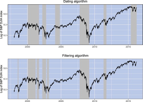
Table 2 reports the descriptive statistics of the bull and bear market states identified by the two algorithms. The descriptive statistics of bull and bear states depend on the choice of the algorithm for detecting the turning points between the market states. Despite the differences, the descriptive statistics share many similarities. The first similarity is that bull markets tend to be longer than bear markets. Regardless of the choice of algorithm, the average bull market duration exceeds the average bear market duration by a factor of 2.7. The second similarity is that all bull markets exhibit a positive mean return, while all bear markets have a negative mean return. Finally, the third similarity is that the market volatility during bear states is almost double the volatility during bull states. In sum, the descriptive statistics suggest a clear-cut conclusion that the bull market refers to the high-return, low-volatility state, whereas the bear market refers to the low-return, high-volatility state of the stock market.

Table 2. Descriptive statistics of bull and bear markets. Duration is measured in the number of months.

	Dating algorithm		Filtering algorithm
Statistics	Bull	Bear	Bull	Bear
Number of phases	6	6	8	7
Minimum duration	5.81	5.14	1.67	3.29
Average duration	25.29	9.52	22.92	8.37
Maximum duration	43.38	16.90	54.95	16.90
Mean return	1.05	−1.39	1.10	−2.32
Standard deviation	3.30	5.42	3.25	5.99

Note: Mean return is the monthly percentage return, and standard deviation is the monthly percentage standard deviation.

3.2. Volatility forecast accuracy across horizons

We remind the reader that our total sample of intraday stock price data covers the period from January 2, 1998, to December 31, 2016. The period from January 2, 1998, to December 31, 1999 (2 years), is used as the initial in-sample period. Consequently, the out-of-sample period in our study is from January 2, 2000, to December 31, 2016 (17 years), which covers several interchanging bull and bear market states.

All forecasts are obtained using an expanding window scheme. Specifically, given a selected forecasting model, we perform out-of-sample volatility forecasting for every stock in our data set. First, the parameters of a model are estimated using in-sample observations $[1,2,\dots ,t]$, t<T, where T denotes the number of observations in the total sample. Then, the volatility is forecasted for 200 days by performing 200 rolling one-day-ahead forecasts. Next, we expand the in-sample period by one day (it becomes $[1,2,\dots ,t+1]$), reestimate the model parameters, and repeat the forecasting procedure.

At the end of the forecasting process, the forecasted daily volatilities are aggregated into weekly volatilities. That is, for each time t, we obtain 40 weekly volatility forecasts ${\hat{\sigma }}_{t,h}$, $h\in [1,2,\dots ,40]$. Similarly, we aggregate daily realized volatilities into weekly realized volatilities, and for each time t, we obtain realized volatilities $R{V}_{t,h}$ for the next 40 consecutive weeks. Then, given ${\hat{\sigma }}_{t,h}$ and $R{V}_{t,h}$, we estimate the unconditional forecast accuracy (that is, the forecast accuracy over all market states) and the forecast accuracy conditional on the bull and bear states. The unconditional forecast accuracy is estimated using equation (22(22) $P\left(h\right)=1-\frac{\sum _{t=1}^M{\left(R{V}_{t,h}-{\hat{\sigma }}_{t,h}\right)}^2}{\sum _{t=1}^M{\left(R{V}_{t,h}-{\overline{RV}}_{t,h}\right)}^2}=1-\frac{SSE\left(h\right)}{TSS\left(h\right)},$(22) ). Over the bull and bear states of the market, conditional forecast accuracy is computed as (30) $\begin{array}{rl}{P}_{\mathrm{B}\mathrm{u}\mathrm{l}\mathrm{l}}\left(h\right)& =1-\frac{\sum _{t=1}^M{\left(R{V}_{t,h}-{\hat{\sigma }}_{t,h}\right)}^2{\text{𝟙}}_{t\in \mathrm{B}\mathrm{u}\mathrm{l}\mathrm{l}}}{\sum _{t=1}^M{\left(R{V}_{t,h}-{\overline{RV}}_{t,h}\right)}^2{\text{𝟙}}_{t\in \mathrm{B}\mathrm{u}\mathrm{l}\mathrm{l}}},\end{array}$(30) (31) $\begin{array}{rl}{P}_{\mathrm{B}\mathrm{e}\mathrm{a}\mathrm{r}}\left(h\right)& =1-\frac{\sum _{t=1}^M{\left(R{V}_{t,h}-{\hat{\sigma }}_{t,h}\right)}^2{\text{𝟙}}_{t\in \mathrm{B}\mathrm{e}\mathrm{a}\mathrm{r}}}{\sum _{t=1}^M{\left(R{V}_{t,h}-{\overline{RV}}_{t,h}\right)}^2{\text{𝟙}}_{t\in \mathrm{B}\mathrm{e}\mathrm{a}\mathrm{r}}},\end{array}$(31) where ${\text{𝟙}}_{t\in \mathrm{B}\mathrm{u}\mathrm{l}\mathrm{l}}$ (${\text{𝟙}}_{t\in \mathrm{B}\mathrm{e}\mathrm{a}\mathrm{r}}$) denotes the indicator function that takes one if the market is in a bull (bear) state on date t and zero otherwise.⁸ Note that in the equations for $P_{\mathrm{B}\mathrm{u}\mathrm{l}\mathrm{l}}\left(h\right)$ and $P_{\mathrm{B}\mathrm{e}\mathrm{a}\mathrm{r}}\left(h\right)$, the value of ${\overline{RV}}_{t,h}$ does not depend on the state of the market. That is, the amount of variation in weekly realized volatility is always computed with respect to its mean value in the total out-of-sample period (which is largely equivalent to using the historical long-run mean value of weekly realized volatility if the out-of-sample period is sufficiently long).

Having computed the volatility forecast accuracies for every stock in our data set and every forecast horizon, we compute the corresponding p-values of the individual predictive ability tests. Finally, for all states of the market and the bull and bear states separately, we compute the average forecast accuracies over all stocks, as well as the p-values of the combined predictive ability test. Figure 2 plots the average volatility forecast accuracies and p-values of the combined predictive ability test versus the forecast horizon for the EWMA and GARCH models. These two models use only daily return data to forecast volatility. Figure 3 plots the average volatility forecast accuracies and p-values of the combined predictive ability test versus the forecast horizon for the HAR-RV and RealGARCH models. The latter two models use high-frequency data to forecast future volatility.

Figure 2. Average volatility forecast accuracies and p-values of the combined predictive ability test versus the forecast horizon for the EWMA and GARCH models. Bull and bear states of the market are detected using the dating algorithm. All curves are constructed using $R{V}_t^{ON}$ as the measure of realized volatility.

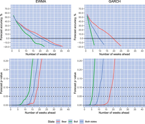
Figure 3. Average volatility forecast accuracies and p-values of the combined predictive ability test versus the forecast horizon for the HAR-RV and RealGARCH models. Bull and bear states of the market are detected using the dating algorithm. All curves are constructed using $R{V}_t^{ON}$ as the measure of realized volatility.

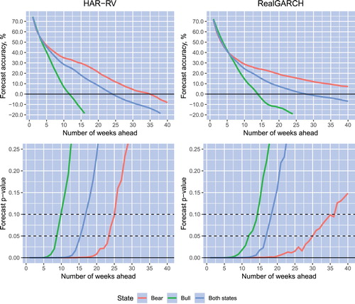
Specifically, the blue lines in Figures 2 and 3, top panels, show the models' average unconditional forecast accuracy, whereas the green (red) lines show the average forecast accuracy conditional on the bull (bear) state of the market. Bull and bear states of the market are detected using the dating algorithm of Pagan and Sossounov (2003). The lines in the bottom panels in the figures depict the p-values of the combined predictive ability test for the unconditional forecast accuracy and the forecast accuracy conditional on the bull and bear states of the market using the blue, green, and red lines, respectively. All curves are constructed using $R{V}_t^{ON}$ as the measure of realized volatility.

On the basis of the results reported in Figures 2 and 3, the following observations can be made. First, consider the unconditional forecast accuracy. Note that, regardless of the choice of volatility model, forecast accuracy is spread highly unevenly across horizons, and the accuracy decreases quickly as the horizon lengthens. Using a significance level of 10%, the horizon of volatility predictability is 10–11 weeks for the GARCH model and 16–18 weeks for the EWMA, HAR-RV, and RealGARCH models. The forecast accuracy gains provided by intraday data are largest for the shortest horizon and diminish quickly when the horizon increases. For instance, compared to the forecast accuracy provided by the EWMA model (for a visual comparison, see also Figure 4, Panel A: Both states), the gains in one-week-ahead volatility forecasting amount to almost 20%, whereas the gains decline to approximately 5% beyond the 10-week horizon.

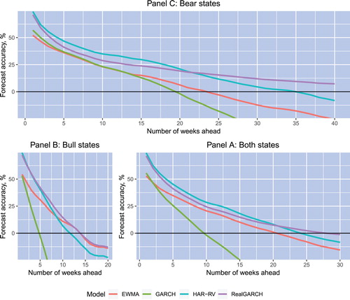
Figure 4. Average volatility forecast accuracies over both states of the market and over bull and bear states separately. Bull and bear states of the market are detected using the dating algorithm. All curves are constructed using $R{V}_t^{ON}$ as the measure of realized volatility.

Second, consider the volatility forecast accuracy conditional on the state of the market. Note that for the majority of volatility models, the horizon of volatility predictability is much longer when the market is in a bear state than when it is in a bull state. Take, as an example, the RealGARCH (HAR-RV) model. Note that at a significance level of 10%, the horizon of volatility predictability extends to 35 (25) weeks when the market is in a bear state. In contrast, the horizon of volatility predictability is limited to only 14 (10) weeks when the market is in a bull state. The EWMA model shows the least difference between the horizons of volatility predictability conditional on the state of the market. For this model, the horizon of volatility predictability amounts to 13 (18) weeks when the market is in a bull (bear) state.

Regardless of the forecast horizon length, the GARCH model forecasts volatility with higher accuracy when the market is in a bear state than when it is in a bull state. The forecast accuracy of the other three models does not depend on the market state when the horizon is rather short. For example, in the EWMA model, over horizons up to 2-3 weeks, forecast accuracy is almost identical in both states of the market. Similarly, over short horizons that are limited to approximately 4-5 weeks, volatility forecast accuracy in the RealGARCH and HAR-RV models effectively does not depend on the state of the market. However, beyond a 5-week horizon, volatility forecast accuracy diminishes very quickly with the lengthening of the horizon when the market is in a bull state. In contrast, when the market is in a bear state, volatility forecast accuracy decreases at a slow rate when the horizon lengthens.

Figure 4 plots the average volatility forecast accuracies over all states of the market and over bull and bear states separately. In particular, for the sake of visual comparison, Panels A, B, and C in this figure plot the average volatility forecast accuracies provided by each volatility model over both states and the bull and bear states of the market, respectively. It is tempting to compare the volatility forecast accuracies of the competing models based on their average forecast accuracies over all stocks in the data set. However, an average forecast accuracy can be misleading because it can be heavily influenced by outliers. More precise evidence on the relative performance of the models comes from a sequence of tests on the combined null hypothesis of inferiority of the forecast accuracy of a given model versus the forecast accuracy of an alternative model. The results of these tests are reported in Table 3. In particular, for every volatility forecasting model, this table reports the p-values associated with the combined null hypothesis of inferiority of this model versus each competing model. The p-values of the combined null of inferiority are estimated over all states of the market and over bull and bear states separately. Bull and bear states of the market are detected using the dating algorithm of Pagan and Sossounov (2003). The estimator $R{V}_t^{ON}$ is used as the measure of realized volatility.

Table 3. P-values associated with the combined null hypothesis of inferiority of a selected model versus each competing model.

	EWMA versus			GARCH versus			RealGARCH versus			HAR-RV versus
Horizon	GARCH	RealGARCH	HAR-RV	EWMA	RealGARCH	HAR-RV	EWMA	GARCH	HAR-RV	EWMA	GARCH	RealGARCH
Panel A: All states
1	0.87	1.00	1.00	0.00	1.00	1.00	0.00	0.00	0.97	0.00	0.00	0.00
2	0.48	1.00	1.00	0.05	1.00	1.00	0.00	0.00	0.86	0.00	0.00	0.06
3	0.20	1.00	1.00	0.23	1.00	1.00	0.00	0.00	0.88	0.00	0.00	0.03
4	0.09	0.97	1.00	0.43	0.99	1.00	0.00	0.00	0.90	0.00	0.00	0.02
5	0.04	0.88	1.00	0.53	0.96	1.00	0.00	0.00	0.81	0.00	0.00	0.02
10	0.02	0.36	0.89	0.63	0.85	0.99	0.13	0.00	0.58	0.08	0.00	0.08
15	0.01	0.46	0.81	0.58	0.90	0.99	0.21	0.00	0.41	0.14	0.00	0.11
20	0.01	0.53	0.68	0.64	0.93	0.98	0.21	0.00	0.29	0.16	0.00	0.18
25	0.01	0.61	0.68	0.69	0.95	0.96	0.23	0.00	0.17	0.24	0.00	0.31
30	0.01	0.69	0.72	0.69	0.96	0.98	0.22	0.00	0.19	0.22	0.00	0.47
Panel B: Bull states
1	0.09	1.00	1.00	0.17	1.00	1.00	0.00	0.00	0.68	0.00	0.00	0.00
2	0.01	1.00	1.00	0.59	1.00	1.00	0.00	0.00	0.16	0.00	0.00	0.02
3	0.00	0.97	1.00	0.71	1.00	1.00	0.00	0.00	0.08	0.00	0.00	0.04
4	0.00	0.78	0.97	0.80	1.00	1.00	0.00	0.00	0.05	0.00	0.00	0.03
5	0.00	0.52	0.82	0.78	1.00	0.99	0.02	0.00	0.03	0.04	0.00	0.05
10	0.00	0.11	0.17	0.84	0.99	0.86	0.34	0.00	0.04	0.51	0.00	0.05
15	0.00	0.11	0.12	0.82	0.98	0.84	0.39	0.00	0.06	0.53	0.00	0.09
20	0.00	0.12	0.24	0.78	0.99	0.88	0.42	0.00	0.09	0.55	0.00	0.14
Panel C: Bear states
1	1.00	1.00	1.00	0.00	1.00	1.00	0.00	0.00	0.91	0.00	0.00	0.00
2	0.91	1.00	1.00	0.00	0.99	1.00	0.00	0.00	0.81	0.00	0.00	0.02
3	0.79	0.97	1.00	0.01	0.91	1.00	0.00	0.00	0.85	0.00	0.00	0.05
4	0.61	0.74	1.00	0.04	0.71	1.00	0.00	0.00	0.87	0.00	0.00	0.03
5	0.48	0.67	0.99	0.06	0.37	0.97	0.00	0.03	0.87	0.00	0.00	0.02
10	0.61	0.58	0.97	0.06	0.17	0.87	0.00	0.02	0.56	0.00	0.01	0.02
15	0.50	0.58	0.97	0.06	0.51	0.94	0.00	0.01	0.51	0.01	0.01	0.05
20	0.36	0.74	0.94	0.08	0.63	0.93	0.01	0.01	0.14	0.01	0.01	0.23
25	0.23	0.82	0.93	0.26	0.77	0.90	0.04	0.01	0.04	0.01	0.01	0.52
30	0.15	0.87	0.92	0.32	0.77	0.91	0.02	0.01	0.10	0.04	0.00	0.59
35	0.10	0.90	0.89	0.50	0.81	0.94	0.06	0.01	0.12	0.03	0.00	0.64
40	0.10	0.92	0.88	0.49	0.84	0.92	0.04	0.00	0.06	0.03	0.00	0.83

Notes: Bold text highlights p-values that are statistically significant at the 10% level. Bull and bear states of the market are detected using the dating algorithm. The estimator $R{V}_t^{ON}$ is used as the measure of realized volatility.

Based on the results reported in Table 3, the following comments can be made regarding the relative performance of the competing models. First, it comes as no surprise that the EWMA and GARCH models are not superior to the RealGARCH and HAR-RV models. In particular, the combined null hypothesis of inferiority of the EWMA and GARCH models versus the RealGARCH and HAR-RV models remains plausible. The EWMA model is superior to the GARCH model in bull states of the market and over all states of the market beyond a 4-week horizon. On the other hand, the GARCH model is superior to the EWMA model over all states of the market at fairly short horizons, that is, those limited to 2 weeks. The GARCH model is also superior to the EWMA model in bear states of the market over horizons up to 20 weeks. It is interesting to note that this conclusion appears despite the fact that the average forecast accuracies of the EWMA and GARCH models in Figure 4, Panel C: Bear states appear to be alike.

The RealGARCH and HAR-RV models are superior to the GARCH model regardless of the forecast horizon length and the market state. These two models are also superior to the EWMA model in bear states of the market over all forecast horizons. However, in bull states of the market, we can reject the combined null hypothesis of inferiority of these models to the EWMA model only over horizons that are shorter than 5–10 weeks. In other words, it is plausible that in bull states of the market over horizons beyond 10 weeks, the EWMA model delivers a forecast accuracy that is similar to that of the RealGARCH and HAR-RV models.

Regarding the comparative accuracy of the RealGARCH and HAR-RV models, the results in Table 3 suggest that over horizons that are shorter than 10–20 weeks, the HAR-RV model is superior to the RealGARCH model in bear states of the market and over all market states. Nonetheless, in bear states of the market over horizons that are longer than 20–25 weeks, the RealGARCH model is superior to the HAR-RV model. In bull states of the market, the results on the relative performance of the RealGARCH and HAR-RV models seem to be paradoxical. Specifically, in bull states of the market, both the combined null hypothesis of the inferiority of the RealGARCH model to the HAR-RV model and the combined null hypothesis of the inferiority of the HAR-RV model to the RealGARCH model are rejected. However, the reader is reminded that the rejection of the combined null hypothesis leads to the conclusion that at least one of the individual alternative null hypotheses is true. Consequently, there is evidence that in bull states of the market, for some stocks in our data set, the RealGARCH model is superior to the HAR-RV model, but for some other stocks, the opposite – namely, that the HAR-RV model is superior to the RealGARCH model – is true. Note, in addition, that in bull states of the market, the average forecast accuracy of the RealGARCH model is close to that of the HAR-RV model (see Figure 4, Panel B: Bull states).

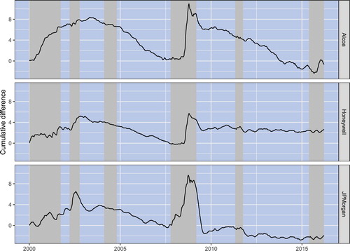
Overall, our results indicate that, generally, volatility forecast accuracy is state dependent and is higher (lower) in bear (bull) states of the market. For the sake of additional illustration, we employ a simple graphical diagnostic tool⁹ that makes it easy to demonstrate how volatility forecast accuracy depends on the state of the market. In particular, to monitor the predictive power of a volatility forecasting model, we use the cumulative difference between the sum of the forecast absolute errors provided by the mean value of realized volatility (which is basically similar to computing forecast errors from the historical mean model) and the forecasted volatility $CUDI{F}_t=\sum _{s=1}^t\left(\left|R{V}_{s,h}-{\overline{RV}}_{s,h}\right|-\left|R{V}_{s,h}-{\hat{\sigma }}_{s,h}\right|\right),t\le M.$ From a visual examination of the graph of $CUDI{F}_t$, it is easy to discern in which periods a volatility model provides a better forecast than the historical mean model. Specifically, in periods when $CUDI{F}_t$ increases, the volatility model provides better predictions; in periods when it decreases, the volatility model has worse predictive performance than the historical mean model.

Figure 5 plots $CUDI{F}_t$ in forecasting the 10th-week volatility of the Alcoa, Honeywell International, and JPMorgan Chase stocks using the EWMA model. Note that for each stock, $CUDI{F}_t$ tends to increase when the market is in a bear state. In contrast, $CUDI{F}_t$ tends to decrease or stay at approximately the same level when the market is in a bull state. That is, the plots in this figure provide a clear-cut illustration of the fact that volatility forecast accuracy is state dependent.

Figure 5. The figure plots $CUDI{F}_t=\sum _{s=1}^t(|R{V}_{s,10}-{\overline{RV}}_{s,10}|-|R{V}_{s,10}-{\hat{\sigma }}_{s,10}|)$ for forecasting 10th-week volatility of the Alcoa, Honeywell International, and JPMorgan Chase stocks using the EWMA model. $|R{V}_{s,10}-{\overline{RV}}_{s,10}|$ is the absolute error in forecasting volatility for the 10th week using the mean value of the realized volatility, while $|R{V}_{s,10}-{\hat{\sigma }}_{s,10}|$ is the absolute error in forecasting volatility for the 10th week using the EWMA model. Shaded areas indicate bear market states. Bull and bear states of the market are detected using the dating algorithm.

3.3. Robustness tests

The results reported in Figures 2–4 and Table 3 are obtained using the whole out-of-sample period from 2000 to 2016 and the following model specifications: the estimator $R{V}_t^{ON}$ is used as the measure of realized volatility; bull and bear states of the market are detected using the dating algorithm; the forecast accuracy is measured using the weekly aggregation of daily volatility; and the forecasting is produced using the expanding window scheme. We subject our results to a series of robustness tests to verify that our core findings are robust to various alternative specifications. Due to space limitations, the results of our numerous robustness tests are reported in a separate online appendix. Below, we only briefly mention these results.

First, virtually the same results as those reported in this paper are obtained by either replacing the measure $R{V}_t^{ON}$ with the measure $R{V}_t^{HL}$ or by using the filtering algorithm to detect the bull and bear states of the market instead of the dating algorithm. Second, we evaluate the forecast accuracy on a daily basis without weekly aggregation. On a daily basis, the results on the volatility forecast accuracy versus forecast horizon length are qualitatively similar to those with weekly aggregation. The quantitative comparison of the results with and without weekly aggregation reveals that, without weekly aggregation, the volatility forecast accuracy is reduced by approximately 5% when the forecast horizon is relatively short. Otherwise, the volatility forecast accuracy is the same with and without weekly aggregation. We conjecture that the reduction in the forecast accuracy over short horizons can be attributed to the presence of the day-of-the-week volatility effect mentioned in Section 2.5.

Third, qualitatively similar results are obtained for volatility forecasting using the rolling window scheme, where the window size equals the length of the initial in-sample period. However, compared to that of forecasting with the expanding window scheme, the forecast accuracy is generally reduced with the rolling window scheme. The reduction is especially notable in bear states of the market. For the HAR-RV model, the deterioration of the forecast accuracy is substantial in all states of the market. The intuition for this result can be explained as follows. Stock market dynamics are different in bull and bear states of the market. Suppose that the market is in a bull state. In this case, using a relatively short rolling window allows a forecasting model to closely capture the market dynamics, but the model becomes unprepared to forecast effectively when a bear market begins. Bear markets have much shorter durations than bull markets, and therefore, when a model is finally fully tuned to forecast effectively in a bear market, a bull market begins. In addition, the HAR-RV model tries to capture the long memory in realized volatility. For this purpose, a longer estimation window is required.

Fourth and finally, the results reported in this paper are robust in the subsamples of data. Specifically, the results are qualitatively similar in the first (2000–2007) and second (2008–2016) halves of the total out-of-sample period.

4. Conclusions

In this paper, we use a large data set of high-frequency data on individual stocks and a few popular time-series volatility models to comprehensively examine how volatility forecastability varies across bull and bear states of the stock market. Our results suggest that volatility predictability depends strongly on the state of the market.

Specifically, we find that the volatility forecast horizon is considerably longer when the market is in a bear state than when it is in a bull state. For instance, when high-frequency data are used, the horizon of volatility predictability extends to 25–35 weeks when the market is in a bear state. In contrast, the horizon of volatility predictability is limited to only 10–14 weeks when the market is in a bull state. The volatility forecast accuracy is highest for the shortest horizons, when it reaches 75%. Over short horizons, that is, those ranging from 2 to 5 weeks, the forecast accuracy is almost identical in both states of the market. However, beyond a 5-week horizon, the volatility forecast accuracy diminishes very quickly with the lengthening of the horizon when the market is in a bull state. In contrast, when the market is in a bear state, the volatility forecast accuracy decreases at a slow rate as the horizon lengthens.

In our study, we employ the EWMA and GARCH models, which use daily data only, and the RealGARCH and HAR-RV models, which use high-frequency data. We assess the forecast accuracy gains from using high-frequency data and compare the predictive accuracies of the competing models. Our results reveal that the gains provided by high-frequency data are substantial and amount to almost 20% for the shortest horizon. The gains diminish quickly as the horizon lengthens when the market is in a bull state. Conversely, in bear states, the gains persist regardless of the horizon length. We find that the EWMA model is superior (inferior) to the GARCH model in bull (bear) states of the market. The forecasting models that use high-frequency data are clearly superior to the models that use daily data. Our results suggest that the HAR-RV model is generally superior to the RealGARCH model in bear states of the market. In bull states of the market, on the other hand, both models forecast with approximately the same accuracy.

In sum, our study concludes, similarly to the previous studies on return predictability, that volatility predictability is strongest during bad economic times, proxied by bear market states. That is, volatility predictability is greatest when it is most needed, during periods of high turbulence and uncertainty.

Supplemental data

Supplemental data for this article can be accessed at http://dx.doi.org/10.1080/14697688.2020.1725101http://dx.doi.org/10.1080/14697688.2020.1725101.

Disclosure statement

No potential conflict of interest was reported by the author(s).

Notes

1 See, among others, Andersen et al. (1999), Blair et al. (2001), Martens (2002), Andersen et al. (2003), Andersen et al. (2005), Koopman et al. (2005), Andersen et al. (2007), Corsi (2009), Han and Park (2013), Hansen et al. (2014), and Hansen and Huang (2016).

2 Another approach to dating bull and bear markets is based on using a regime-switching model; see, for example, Maheu and McCurdy (2000). However, significant drawbacks of this approach are as follows. First, a detected turning point usually does not coincide with a historical peak or trough in stock prices. Second, using only two states in a regime-switching model is usually not enough to describe the number of regimes in a stock market; see Maheu et al. (2012).

3 A cycle denotes two subsequent phases, either an upswing and consequent downswing or a downswing and consequent upswing.

4 Hansen et al. (2012) advocate that the log-linear specification of the RealGARCH model should be preferred to the linear specification.

5 We remind the reader that the HAR-RV model predicts realized volatility. Therefore, regarding the HAR-RV model, in the subsequent exposition, ${\hat{\sigma }}_{t,h}$ must be replaced by ${\widehat{RV}}_{t,h}$.

6 In particular, we estimate the optimal block length for each column of matrices $\mathbf{S}\mathbf{S}\mathbf{E}$ and $\mathbf{T}\mathbf{S}\mathbf{S}$. The stationary block-bootstrap method is implemented using the average block length over $2k$ estimated optimal block lengths.

7 https://finance.yahoo.com/

8 The motivation for our computation of conditional forecast accuracy is as follows. Most often, at time t, the state of the market is known. In contrast, at time t, the state of the market in week h in the future is unknown. Therefore, conditional forecast accuracy is computed under the assumption that the forecaster possesses the knowledge of the market state at time t but is completely ignorant of the state of the market in week h in the future.

9 A similar graphical diagnostic tool is suggested in Goyal and Welch (2003).

References

- Alford, A.W. and Boatsman, J.R., Predicting long-term stock return volatility: Implications for accounting and valuation of equity derivatives. Account. Rev., 1995, 70, 599–618.
- Andersen, T.G. and Bollerslev, T., Answering the skeptics: Yes, standard volatility models do provide accurate forecasts. Int. Econ. Rev. (Philadelphia), 1998, 39, 885–905.
- Andersen, T.G., Bollerslev, T. and Diebold, F.X., Roughing it up: Including jump components in the measurement, modeling, and forecasting of return volatility. Rev. Econ. Stat., 2007, 89, 701–720.
- Andersen, T.G., Bollerslev, T., Diebold, F.X. and Labys, P., Great realizations. Risk, 2000, 13, 105–108.
- Andersen, T.G., Bollerslev, T., Diebold, F.X. and Labys, P., The distribution of realized exchange rate volatility. J. Am. Stat. Assoc., 2001, 96, 42–55.
- Andersen, T.G., Bollerslev, T., Diebold, F.X. and Labys, P., Modeling and forecasting realized volatility. Econometrica, 2003, 71, 579–625.
- Andersen, T.G., Bollerslev, T. and Lange, S., Forecasting financial market volatility: Sample frequency vis-a-vis forecast horizon. J. Empir. Financ., 1999, 6, 457–477.
- Andersen, T.G., Bollerslev, T. and Meddahi, N., Correcting the errors: Volatility forecast evaluation using high-frequency data and realized volatilities. Econometrica, 2005, 73, 279–296.
- Awartani, B., Corradi, V. and Distaso, W., Assessing market microstructure effects via realized volatility measures with an application to the Dow Jones industrial average stocks. J. Busi. Econ. Stat., 2009, 27, 251–265.
- Bandi, F.M. and Russell, J.R., Separating microstructure noise from volatility. J. Financ. Econ., 2006, 79, 655–692.
- Biscarri, J.G. and de Gracia, F.P., Stock market cycles and stock market development in Spain. Span. Econ. Rev., 2004, 6, 127–151.
- Blair, B.J., Poon, S.H. and Taylor, S.J., Forecasting S&P 100 volatility: The incremental information content of implied volatilities and high-frequency index returns. J. Econom., 2001, 105, 5–26.
- Bollerslev, T., Generalized autoregressive conditional heteroskedasticity. J. Econom., 1986, 31, 307–327.
- Bollerslev, T., Hood, B., Huss, J. and Pedersen, L.H., Risk everywhere: Modeling and managing volatility. Rev. Financ. Stud., 2018, 31, 2729–2773.
- Bollerslev, T. and Wright, J.H., High-frequency data, frequency domain inference, and volatility forecasting. Rev. Econ. Stat., 2001, 83, 596–602.
- Brown, M.B., 400: A method for combining non-independent, one-sided tests of significance. Biometrics, 1975, 31, 987–992.
- Bry, G. and Boschan, C., Cyclical Analysis of Time Series: Selected Procedures and Computer Programs, 1971 (NBER: New York).
- Campbell, J.Y. and Thompson, S.B., Predicting excess stock returns out of sample: Can anything beat the historical average? Rev. Financ. Stud., 2007, 21, 1509–1531.
- Cao, C.Q. and Tsay, R.S., Nonlinear time-series analysis of stock volatilities. J. Appl. Econom., 1992, 7, S165–S185.
- Chauvet, M. and Potter, S., Coincident and leading indicators of the stock market. J. Empir. Financ., 2000, 7, 87–111.
- Cheema, M.A., Nartea, G.V. and Man, Y., Cross-sectional and time series momentum returns and market states. Int. Rev. Financ., 2018, 18, 705–715.
- Christoffersen, P.F. and Diebold, F.X., How relevant is volatility forecasting for financial risk management? Rev. Econ. Stat., 2000, 82, 12–22.
- Corsi, F., A simple approximate long-memory model of realized volatility. J. Financ. Econom., 2009, 7, 174–196.
- Dangl, T. and Halling, M., Predictive regressions with time-varying coefficients. J. Financ. Econ., 2012, 106, 157–181.
- Diebold, F.X. and Mariano, R.S., Comparing predictive accuracy. J. Busi. Econ. Stat., 1995, 13, 134–144.
- Engle, R., New frontiers for ARCH models. J. Appl. Econom., 2002, 17, 425–446.
- Engle, R.F. and Gallo, G.M., A multiple indicators model for volatility using intra-daily data. J. Econom., 2006, 131, 3–27.
- Engle, R. and Patton, A., What good is a volatility model? Quant. Finance, 2001, 1, 237–245.
- Fama, E.F., The behavior of stock-market prices. J. Bus., 1965, 38, 34–105.
- Figlewski, S., Forecasting volatility. Financial Mark. Inst. Instrum., 1997, 6, 1–88.
- Fisher, R.A., Statistical Methods for Research Workers, 1925 (Oliver and Boyd: Edinburgh).
- Fleming, J., Ostdiek, B. and Whaley, R.E., Predicting stock market volatility: A new measure. J. Futures Mark., 1995, 15, 265–302.
- French, K.R. and Roll, R., Stock return variances: The arrival of information and the reaction of traders. J. Financ. Econ., 1986, 17, 5–26.
- Fuertes, A.M., Kalotychou, E. and Todorovic, N., Daily volume, intraday and overnight returns for volatility prediction: Profitability or accuracy? Rev. Quant. Financ. Account., 2015, 45, 251–278.
- Galbraith, J.W. and Kisinbay, T., Content horizons for conditional variance forecasts. Int. J. Forecast., 2005, 21, 249–260.
- Garcia, D., Sentiment during recessions. J. Finance, 2013, 68, 1267–1300.
- Gargano, A., Pettenuzzo, D. and Timmermann, A., Bond return predictability: Economic value and links to the macroeconomy. Manage. Sci., 2017, 65, 508–540.
- Gargano, A. and Timmermann, A., Forecasting commodity price indexes using macroeconomic and financial predictors. Int. J. Forecast., 2014, 30, 825–843.
- Golez, B. and Koudijs, P., Four centuries of return predictability. J. Financ. Econ., 2018, 127, 248–263.
- Gonzalez, L., Powell, J.G., Shi, J. and Wilson, A., Two centuries of bull and bear market cycles. Int. Rev. Econ. Financ., 2005, 14, 469–486.
- Goyal, A. and Welch, I., Predicting the equity premium with dividend ratios. Manage. Sci., 2003, 49, 639–654.
- Green, T.C. and Figlewski, S., Market risk and model risk for a financial institution writing options. J. Finance, 1999, 54, 1465–1499.
- Haas, M. and Liu, J., A multivariate regime-switching GARCH model with an application to global stock market and real estate equity returns. Stud. Nonlinear Dyn. Econ., 2018, 22, 1–27.
- Haas, M., Mittnik, S. and Paolella, M.S., A new approach to Markov-switching GARCH models. J. Financ. Econom., 2004, 2, 493–530.
- Hammerschmid, R. and Lohre, H., Regime shifts and stock return predictability. Int. Rev. Econ. Financ., 2018, 56, 138–160.
- Han, H. and Park, M.D., Comparison of realized measure and implied volatility in forecasting volatility. J. Forecast., 2013, 32, 522–533.
- Hansen, P.R. and Huang, Z., Exponential GARCH modeling with realized measures of volatility. J. Busi. Econ. Stat., 2016, 34, 269–287.
- Hansen, P.R., Huang, Z. and Shek, H.H., Realized GARCH: A joint model for returns and realized measures of volatility. J. Appl. Econom., 2012, 27, 877–906.
- Hansen, P.R. and Lunde, A., A forecast comparison of volatility models: Does anything beat a GARCH(1,1)? J. Appl. Econom., 2005a, 20, 873–889.
- Hansen, P.R. and Lunde, A., A realized variance for the whole day based on intermittent high-frequency data. J. Financ. Econom., 2005b, 3, 525–554.
- Hansen, P.R., Lunde, A. and Voev, V., Realized beta GARCH: A multivariate GARCH model with realized measures of volatility. J. Appl. Econom., 2014, 29, 774–799.
- Harvey, D., Leybourne, S. and Newbold, P., Testing the equality of prediction mean squared errors. Int. J. Forecast., 1997, 13, 281–291.
- Henkel, S.J., Martin, J.S. and Nardari, F., Time-varying short-horizon predictability. J. Financ. Econ., 2011, 99, 560–580.
- Kaminsky, G.L. and Schmukler, S.L., Short-run pain, long-run gain: Financial liberalization and stock market cycles. Rev. Financ., 2008, 12, 253–292.
- Klaassen, F., Improving GARCH volatility forecasts with regime-switching GARCH. In Advances in Markov-switching Models: Applications in Business Cycle Research and Finance, edited by J.D. Hamilton and B. Raj, pp. 223–254, 2002 (Physica-Verlag HD: Heidelberg).
- Koopman, S.J., Jungbacker, B. and Hol, E., Forecasting daily variability of the S&P 100 stock index using historical, realised and implied volatility measurements. J. Empir. Financ., 2005, 12, 445–475.
- Littell, R.C. and Folks, J.L., Asymptotic optimality of Fisher's method of combining independent tests. J. Am. Stat. Assoc., 1971, 66, 802–806.
- Longerstaey, J. and Spencer, M., RiskMetricsTM—technical document. Technical Report, Morgan Guaranty Trust Company, New York, 1996.
- Lunde, A. and Timmermann, A., Duration dependence in stock prices: An analysis of bull and bear markets. J. Busi. Econ. Stat., 2004, 22, 253–273.
- Maheu, J.M. and McCurdy, T.H., Identifying bull and bear markets in stock returns. J. Busi. Econ. Stat., 2000, 18, 100–112.
- Maheu, J.M., McCurdy, T.H. and Song, Y., Components of bull and bear markets: Bull corrections and bear rallies. J. Busi. Econ. Stat., 2012, 30, 391–403.
- Marcucci, J., Forecasting stock market volatility with regime-switching GARCH models. Stud. Nonlinear Dyn. Econom., 2005, 9, 1–53.
- Martens, M., Measuring and forecasting S&P 500 index-futures volatility using high-frequency data. J. Futures Mark., 2002, 22, 497–518.
- Martens, M., van Dijk, D. and de Pooter, M., Forecasting S&P 500 volatility: Long memory, level shifts, leverage effects, day-of-the-week seasonality, and macroeconomic announcements. Int. J. Forecast., 2009, 25, 282–303.
- Martens, M. and Zein, J., Predicting financial volatility: High-frequency time-series forecasts vis-a-vis implied volatility. J. Futures Mark., 2004, 24, 1005–1028.
- Merton, R.C., On estimating the expected return on the market: An exploratory investigation. J. Financ. Econ., 1980, 8, 323–361.
- Pagan, A.R. and Sossounov, K.A., A simple framework for analysing bull and bear markets. J. Appl. Econom., 2003, 18, 23–46.
- Pan, Z., Wang, Y., Wu, C. and Yin, L., Oil price volatility and macroeconomic fundamentals: A regime switching GARCH-MIDAS model. J. Empir. Financ., 2017, 43, 130–142.
- Patton, A., Politis, D.N. and White, H., Correction to “Automatic block-length selection for the dependent bootstrap” by D. Politis and H. White. Econom. Rev., 2009, 28, 372–375.
- Politis, D. and Romano, J., The stationary bootstrap. J. Am. Stat. Assoc., 1994, 89, 1303–1313.
- Politis, D.N. and White, H., Automatic block-length selection for the dependent bootstrap. Econom. Rev., 2004, 23, 53–70.
- Pong, S., Shackleton, M.B., Taylor, S.J. and Xu, X., Forecasting currency volatility: A comparison of implied volatilities and AR(FI)MA models. J. Bank. Financ., 2004, 28, 2541–2563.
- Poon, S.H., A Practical Guide to Forecasting Financial Market Volatility, 2005 (John Wiley & Sons: Chichester).
- Poon, S.H. and Granger, C.W.J., Forecasting volatility in financial markets: A review. J. Econ. Lit., 2003, 41, 478–539.
- Rapach, D.E., Strauss, J.K. and Zhou, G., Out-of-sample equity premium prediction: Combination forecasts and links to the real economy. Rev. Financ. Stud., 2009, 23, 821–862.
- Raunig, B., The longer-horizon predictability of German stock market volatility. Int. J. Forecast., 2006, 22, 363–372.
- Scharth, M. and Medeiros, M.C., Asymmetric effects and long memory in the volatility of Dow Jones stocks. Int. J. Forecast., 2009, 25, 304–327.
- Schmeling, M., Investor sentiment and stock returns: Some international evidence. J. Empir. Financ., 2009, 16, 394–408.
- Sperandeo, V., Principles of Professional Speculation, 1994 (John Wiley & Sons: New York).
- Todorova, N. and Soucek, M., Overnight information flow and realized volatility forecasting. Finance Res. Lett., 2014, 11, 420–428.
- Welch, I. and Goyal, A., A comprehensive look at the empirical performance of equity premium prediction. Rev. Financ. Stud., 2008, 21, 1455–1508.