Bayesian mean–variance analysis: optimal portfolio selection under parameter uncertainty

Abstract

The paper solves the problem of optimal portfolio choice when the parameters of the asset returns distribution, for example the mean vector and the covariance matrix, are unknown and have to be estimated by using historical data on asset returns. Our new approach employs the Bayesian posterior predictive distribution which is the distribution of future realizations of asset returns given the observable sample. The parameters of posterior predictive distributions are functions of the observed data values and, consequently, the solution of the optimization problem is expressed in terms of data only and does not depend on unknown quantities. By contrast, the optimization problem of the traditional approach is based on unknown quantities which are estimated in the second step, and lead to a suboptimal solution. We also derive a very useful stochastic representation of the posterior predictive distribution whose application not only gives the solution of the considered optimization problem, but also provides the posterior predictive distribution of the optimal portfolio return which can be used to construct a prediction interval. A Bayesian efficient frontier, the set of optimal portfolios obtained by employing the posterior predictive distribution, is constructed as well. Theoretically and using real data we show that the Bayesian efficient frontier outperforms the sample efficient frontier, a common estimator of the set of optimal portfolios which is known to be overoptimistic.

Keywords:

• Optimal portfolio
• Posterior predictive distribution
• Parameter uncertainty
• Efficient frontier
• Stochastic representation
• Black–Litterman model

JEL Classification:

• C11
• C13
• C44
• C58
• C63

1. Introduction

The fundamental goal of portfolio theory is to allocate optimally investments between different assets. Mean–variance optimization is a quantitative tool which allows one to make this allocation by considering the trade-off between the risk of a portfolio and its return. The basic concepts of modern portfolio theory were developed by Markowitz (1952) who introduced a mean–variance portfolio optimization procedure in which investors incorporate their preferences towards the risk and the expected return to seek the best allocation of wealth. This is attained by selecting portfolios that maximize expected portfolio return subject to achieving a prespecified level of risk or, equivalently, that minimize the variance subject to achieving a prespecified level of expected return. The mean–variance analysis of Markowitz is an important tool for both practitioners and researchers in the financial sector today.

The classical problems and pitfalls of mean–variance analysis are mainly related to extreme weights that often occur when the sample efficient portfolio is constructed. This point was discussed in detail by Merton (1980) who presented an estimator of the instantaneous expected return on the market in a log-normal diffusion price model and showed its slow convergence. Moreover, it was proved that the estimates of the variances and covariances of the asset returns are more accurate than the estimates of the means. Best and Grauer (1991) argued that optimal portfolios are very sensitive to the level of expected returns. Therefore, improving the technique of mean estimation has recently become a key issue of the portfolio optimization problem. The same challenge is also present when the covariance matrix needs to be estimated. To this end, Broadie (1993) showed that the estimated efficient frontier, the set of all mean–variance optimal portfolios, overestimates the expected returns of portfolios for different levels of estimation error. A similar conclusion has also been drawn in more recent studies by Basak et al. (2005), Siegel and Woodgate (2007) and Bodnar and Bodnar (2010).

An alternative approach to deal with the parameter uncertainty in portfolio analysis is to employ the methods of Bayesian statistics (cf. Barry 1974, Brown 1976, Klein and Bawa 1976, Frost and Savarino 1986, Aguilar and West 2000, Rachev et al. 2008, Avramov and Zhou 2010, Sekerke 2015, Bodnar et al. 2017, Bauder et al. 2018, 2019). It is remarkable that the Bayesian approach is potentially more attractive since: (i) it uses prior information about quantities of interest; (ii) it facilitates the use of fast, intuitive, and easily implementable numerical algorithms in order to simulate complex economic quantities; (iii) it accounts for estimation risk and model uncertainty in the portfolio choice problem. First applications of Bayesian statistics to portfolio analysis during the 1970s were completely based on noninformative or data-based priors. Bawa et al. (1979) provided an excellent early survey of such applications. The Bayesian approaches based on the diffusion prior are usually comparable with the classical methods of portfolio selection. However, if some of the risky assets have longer histories than others, then the Bayesian approaches under the diffuse prior lead to different results (see Stambaugh 1997). Jorion (1986) introduced the hyperparameter prior approach in the spirit of the Bayes–Stein shrinkage prior, whereas Black and Litterman (1992) defended an informal Bayesian analysis with economic arguments and equilibrium relations. They derived the Black–Litterman model which leads to more stable and more diversified portfolios than simple mean–variance optimization. Unfortunately, the application of this model requires a broad variety of data, some of which may be hard to find. Recent studies by Pástor (2000) and Pástor and Stambaugh (2000) centred prior beliefs around values implied by asset pricing theories. In particular, Pástor and Stambaugh (2000) investigated the portfolio choices of mean–variance–optimizing investors who use sample evidence to update prior beliefs centred on either the risk-based or characteristic-based pricing models. Tu and Zhou (2010) argued that the investment objective provides a useful prior for portfolio selection and proposed an optimal combination of the naive equally weighted portfolio rule with one of the four sophisticated strategies—the Markowitz (1952) rule, the Jorion (1986) rule, the MacKinlay and Pástor (2000) rule, or the Kan and Zhou (2007) rule—as a way to improve performance. Finally, Kacperczyk and Damien (2011) and Kacperczyk et al. (2013) discussed the application of Bayesian semi-parametric models, while Brandt and Santa-Clara (2006) considered the Bayesian approach in the multi-period optimal portfolio choice problem.

We contribute to the existing literature on optimal portfolio selection by formulating an optimization problem in terms of the posterior predictive distribution and solving it. Using the available information about the development of asset returns which is present in their historical observations, the aim is to construct an optimal portfolio by taking into account investor's preferences. The conventional approach consists of two steps: (i) first, the optimization problem is solved with the solution depending on the unknown parameters of the asset return distribution; (ii) second, the optimal portfolio weights, which are the solutions of the optimization problem, are estimated by applying the historical observations of the asset returns. The second step is always needed in practical applications, since the expression of optimal portfolio weights resulting from the first step usually involve the unknown population parameters of the asset return distribution. Replacing these parameters by their sample estimators leads to additional uncertainty in the decision process which has been ignored for a long time in financial literature. It is important to note that following this two-step approach, the obtained solution is only suboptimal and it can deviate considerably from the optimal (population) portfolio obtained in the first stage.

In this paper, we propose a new approach, where the solution of the investor's optimization problem is obtained by employing the posterior predictive distribution which takes parameter uncertainty into account before the optimal portfolio choice problem is solved. As a result, its solution is presented in terms of historical data and is independent of the unknown parameters of the asset returns distribution. Consequently, it can be directly applied in practice and, in contrast to the conventional approach, it is optimal.

The rest of the paper is organized as follows. Main theoretical results are given in Section 2. Here, we characterize the posterior predictive distribution of the asset returns by developing a very helpful stochastic representation (Theorem 1). This stochastic representation provides not only a way how the future realization of portfolio returns can be simulated, but it is also used to derive the first two moments needed for the considered optimization problem. Section 2.2 deals with constructing optimal portfolios by maximizing the posterior mean–variance utility function, while the expression of the Bayesian efficient frontier is derived in Section 2.3. In Section 2.4 the optimal portfolio choice problem is solved by employing the informative conjugate prior, that can be considered as an extension of the Black–Litterman model, a popular approach in the financial literature. Section 3 presents a numerical comparison of the two Bayesian approaches between each other as well as to methods based on frequentist statistics. The theoretical results are implemented in an empirical study in Section 4, while Section 5 provides a conclusion. The technical derivations are given in an appendix.

2. Mean–variance analysis under parameter uncertainty

2.1. Posterior predictive distribution

Let ${\mathbf{\text{X}}}_t$ denote the k-dimensional vector of returns on asset at time t. Assume that a sample of size n of asset returns ${\mathbf{\text{x}}}_{t-n},\dots ,{\mathbf{\text{x}}}_{t-1}$, realizations of ${\mathbf{\text{X}}}_{t-n},\dots ,{\mathbf{\text{X}}}_{t-1}$, is available which provides the information set ${\mathcal{F}}_{t-1}$ and let ${\mathbf{\text{x}}}_{(t-1)}=({\mathbf{\text{x}}}_{t-n},\dots ,{\mathbf{\text{x}}}_{t-1})$ be the observation matrix at time t−1. Consequently, an investor makes a decision by optimizing preferences using information ${\mathcal{F}}_{t-1}$.

Before the decision problem is formulated in Section 2.2, we first derive the predictive posterior distribution $p\left({\mathbf{\text{X}}}_t|{\mathbf{\text{x}}}_{(t-1)}\right)$ of ${\mathbf{\text{X}}}_t$ given the previous observation of asset returns summarized in ${\mathbf{\text{x}}}_{(t-1)}$. The derivation of $p\left({\mathbf{\text{X}}}_t|{\mathbf{\text{x}}}_{(t-1)}\right)$ is based on the methods of Bayesian statistics which provide well-established techniques for providing inferences of future realizations of asset returns given information ${\mathcal{F}}_{t-1}$.

In the following we assume that the asset returns ${\mathbf{\text{X}}}_1,{\mathbf{\text{X}}}_2,\dots$ are infinitely exchangeable and multivariate centred spherically symmetric (see, Bernardo and Smith 2000, Section 4.4 for the definition and properties). This assumption is very general and it implies that neither the unconditional distribution of the asset returns is normal nor that they are independently distributed. Moreover, the unconditional distribution of the asset returns appears to be heavy-tailed which is usually observed for financial data (see, e.g. Bradley and Taqqu 2003).

Parameterizing the density function of ${\mathbf{\text{X}}}_{(t-1)}=({\mathbf{\text{X}}}_{t-n},\dots ,{\mathbf{\text{X}}}_{t-1})$ by the parameter $\mathit{\theta }$, the posterior distribution of $\mathit{\theta }$ is obtained by applying the Bayes theorem and it is given by (1) $\pi \left(\mathit{\theta }|{\mathbf{\text{x}}}_{(t-1)}\right)\propto f\left({\mathbf{\text{x}}}_{(t-1)}|\mathit{\theta }\right)\pi \left(\mathit{\theta }\right),$(1) where $\pi \left(\mathit{\theta }\right)$ denotes the prior and $f\left({\mathbf{\text{x}}}_{(t-1)}|\mathit{\theta }\right)$ is the likelihood function of ${\mathbf{\text{X}}}_{(t-1)}$. The posterior distribution $\mathit{\theta }$ is then used to derive the posterior predictive distribution of the portfolio return at time t expressed as (2) $X_{p,t}={\mathbf{\text{w}}}^{\mathrm{\top }}{\mathbf{\text{X}}}_t,$(2) where $\mathbf{\text{w}}=(w_1,\dots ,w_p{)}^{\mathrm{\top }}$ is the k-dimensional vector of portfolio weights.

The posterior distribution (1(1) $\pi \left(\mathit{\theta }|{\mathbf{\text{x}}}_{(t-1)}\right)\propto f\left({\mathbf{\text{x}}}_{(t-1)}|\mathit{\theta }\right)\pi \left(\mathit{\theta }\right),$(1) ) is employed in the derivation of the posterior predictive distribution as follows: (3) $f\left(x_{p,t}|{\mathbf{\text{x}}}_{(t-1)}\right)={\int }_{\mathit{\theta }\in \mathbf{\Theta }}f\left(x_{p,t}|\mathit{\theta }\right)\pi \left(\mathit{\theta }|{\mathbf{\text{x}}}_{(t-1)}\right)\mathrm{d}\mathit{\theta }.$(3) Due to the integration present in the definition of the posterior predictive distribution, it is possible to obtain the analytical expression of $f\left(x_{p,t}|{\mathbf{\text{x}}}_{(t-1)}\right)$ only in very rare cases. Moreover, the integration in (3(3) $f\left(x_{p,t}|{\mathbf{\text{x}}}_{(t-1)}\right)={\int }_{\mathit{\theta }\in \mathbf{\Theta }}f\left(x_{p,t}|\mathit{\theta }\right)\pi \left(\mathit{\theta }|{\mathbf{\text{x}}}_{(t-1)}\right)\mathrm{d}\mathit{\theta }.$(3) ) could also be high-dimensional, which makes the application of numerical methods very time consuming and also questions the quality of their numerical approximation. In Theorem 1, we derive a stochastic representation for the posterior predictive distribution $f\left(x_{p,t}|{\mathbf{\text{x}}}_{(t-1)}\right)$ which can be very easily used to draw samples from this distribution as well as to compute its expected value and variance analytically. Finally, it has to be noted that the application of the stochastic representation describing the distribution of random quantities has been used both in the frequentist statistics (see, e.g. Givens and Hoeting 2012, Gupta et al. 2013) and in the Bayesian statistics (cf. Bodnar et al. 2017).

Theorem 1

Let ${\mathbf{X}}_1,{\mathbf{X}}_2,\dots$ be infinitely exchangeable and multivariate centred spherically symmetric. Let $\pi \left(\mathit{\theta }\right)=|\mathbf{F}{|}^{1/2}$ be Jeffreys' prior where $|\mathbf{A}|$ denotes the determinant of a square matrix $\mathbf{A}$ and $\mathbf{F}=-\mathbb{E}\left({\mathrm{\partial }}^2\log \left(f\right({\mathbf{x}}_{(t-1)}|\mathit{\theta }\left)\right)/\mathrm{\partial }\mathit{\theta }\mathrm{\partial }{\mathit{\theta }}^{\mathrm{\top }}\right)$ is the Fisher information matrix. Assume n>k. Then the stochastic representation of the random variable ${\hat{X}}_{p,t}$ whose density is the posterior predictive distribution (3(3) $f\left(x_{p,t}|{\mathbf{\text{x}}}_{(t-1)}\right)={\int }_{\mathit{\theta }\in \mathbf{\Theta }}f\left(x_{p,t}|\mathit{\theta }\right)\pi \left(\mathit{\theta }|{\mathbf{\text{x}}}_{(t-1)}\right)\mathrm{d}\mathit{\theta }.$(3) ) is given by $\begin{array}{rl}{\hat{X}}_{p,t}& \stackrel{d}{=}{\mathbf{w}}^{\mathrm{\top }}{\overline{\mathbf{x}}}_{t-1}+\sqrt{{\mathbf{w}}^{\mathrm{\top }}{\mathbf{S}}_{t-1}\mathbf{w}}\\ & \times \left(\frac{{\tau }_1}{\sqrt{n(n-k)}}+\sqrt{1+\frac{{\tau }_1^2}{n-k}}\frac{{\tau }_2}{\sqrt{n-k+1}}\right),\end{array}$ where (4) $\begin{array}{r}{\overline{\mathbf{x}}}_{t-1}=\frac{1}{n}\sum _{i=t-n}^{t-1}{\mathbf{x}}_i\mathrm{a}\mathrm{n}\mathrm{d}{\mathbf{S}}_{t-1}=\sum _{i=t-n}^{t-1}({\mathbf{x}}_i-{\overline{\mathbf{x}}}_{t-1})({\mathbf{x}}_i-{\overline{\mathbf{x}}}_{t-1}{)}^{\mathrm{\top }},\end{array}$(4) and ${\tau }_1$, ${\tau }_2$ are independent with ${\tau }_1\sim t_{n-k}$ and ${\tau }_2\sim t_{n-k+1}$. The symbol ‘$\stackrel{d}{=}$’ denotes the equality in distribution.

The proof of Theorem 1 is given in the appendix. Its results provide an easy way how a random sample from the posterior distribution of $f\left(x_{p,t}|{\mathbf{\text{x}}}_{(t-1)}\right)$ can be simulated as summarized in Algorithm 1:

The generated sample ${\hat{X}}_{p,t}^{\left(1\right)},\dots ,{\hat{X}}_{p,t}^{\left(B\right)}$ is used to calculate important characteristics of the distribution $f\left(x_{p,t}|{\mathbf{\text{x}}}_{(t-1)}\right)$, like the mean, the variance, the credible interval, etc. To this end, we note that the condition n>k ensures that ${\mathbf{\text{S}}}_t$ is positive definite and, hence, it is invertible.

Another important application of Theorem 1 provides us with the analytical expression of the expected value and the variance of the posterior predictive distribution $f\left(x_{p,t}|{\mathbf{\text{x}}}_{(t-1)}\right)$. These findings are formulated in Corollary 1.

Corollary 1

Under the conditions of Theorem 1, let n−k>2. Then: (5) $\mathbb{E}\left({\mathbf{w}}^{\mathrm{\top }}{\mathbf{X}}_t|{\mathbf{x}}_{(t-1)}\right)={\mathbf{w}}^{\mathrm{\top }}{\overline{\mathbf{x}}}_{t-1}$(5) and (6) $\begin{array}{rl}& \mathbb{V}ar\left({\mathbf{w}}^{\mathrm{\top }}{\mathbf{X}}_t|{\mathbf{x}}_{(t-1)}\right)=c_{k,n}{\mathbf{w}}^{\mathrm{\top }}{\mathbf{S}}_{t-1}\mathbf{w}\mathrm{w}\mathrm{i}\mathrm{t}\mathrm{h}\\ & c_{k,n}=\frac{1}{n-k-1}+\frac{2n-k-1}{n(n-k-1)(n-k-2)}.\end{array}$(6)

The proof of Corollary 1 is given in the appendix. Its results are used in the next section where the expressions of optimal portfolio weights are given.

2.2. Mean–variance optimal portfolios

The mean–variance investor constructs an optimal portfolio at time t−1 for the next period by maximizing the mean–variance utility function given by (7) $\begin{array}{rl}U\left(\mathbf{\text{w}}\right)& =\mathbb{E}\left(X_{p,t}|{\mathbf{\text{x}}}_{(t-1)}\right)-\frac{\gamma }{2}\mathbb{V}ar\left(X_{p,t}|{\mathbf{\text{x}}}_{(t-1)}\right)\\ & ={\mathbf{\text{w}}}^{\mathrm{\top }}{\overline{\mathbf{\text{x}}}}_{t-1}-\frac{c_{k,n}\gamma }{2}{\mathbf{\text{w}}}^{\mathrm{\top }}{\mathbf{\text{S}}}_{t-1}\mathbf{\text{w}}\end{array}$(7) under the constraint that the whole wealth is invested into the selected assets, i.e. ${\mathbf{\text{w}}}^{\mathrm{\top }}\mathbf{\text{1}}=1$ where $\mathbf{\text{1}}$ denotes the k-dimensional vector of ones. The quantity $\gamma >0$ stands for the coefficient of the investor's risk aversion and describes the investor's attitude towards risk.

In contrast to the conventional approach that involves the unknown parameters of the asset return distribution in its formulation, the optimization problem in (7(7) $\begin{array}{rl}U\left(\mathbf{\text{w}}\right)& =\mathbb{E}\left(X_{p,t}|{\mathbf{\text{x}}}_{(t-1)}\right)-\frac{\gamma }{2}\mathbb{V}ar\left(X_{p,t}|{\mathbf{\text{x}}}_{(t-1)}\right)\\ & ={\mathbf{\text{w}}}^{\mathrm{\top }}{\overline{\mathbf{\text{x}}}}_{t-1}-\frac{c_{k,n}\gamma }{2}{\mathbf{\text{w}}}^{\mathrm{\top }}{\mathbf{\text{S}}}_{t-1}\mathbf{\text{w}}\end{array}$(7) ) already incorporates the parameter uncertainty by using the available information summarized in the data matrix ${\mathbf{\text{x}}}_{(t-1)}$. As a result, the output of solving (7(7) $\begin{array}{rl}U\left(\mathbf{\text{w}}\right)& =\mathbb{E}\left(X_{p,t}|{\mathbf{\text{x}}}_{(t-1)}\right)-\frac{\gamma }{2}\mathbb{V}ar\left(X_{p,t}|{\mathbf{\text{x}}}_{(t-1)}\right)\\ & ={\mathbf{\text{w}}}^{\mathrm{\top }}{\overline{\mathbf{\text{x}}}}_{t-1}-\frac{c_{k,n}\gamma }{2}{\mathbf{\text{w}}}^{\mathrm{\top }}{\mathbf{\text{S}}}_{t-1}\mathbf{\text{w}}\end{array}$(7) ) is the formula for optimal portfolio weights that could be directly applied in practice, while the estimation of optimal portfolio weights is required in the conventional methods that leads to the suboptimality of the resulting portfolio.

The optimization problem in (7(7) $\begin{array}{rl}U\left(\mathbf{\text{w}}\right)& =\mathbb{E}\left(X_{p,t}|{\mathbf{\text{x}}}_{(t-1)}\right)-\frac{\gamma }{2}\mathbb{V}ar\left(X_{p,t}|{\mathbf{\text{x}}}_{(t-1)}\right)\\ & ={\mathbf{\text{w}}}^{\mathrm{\top }}{\overline{\mathbf{\text{x}}}}_{t-1}-\frac{c_{k,n}\gamma }{2}{\mathbf{\text{w}}}^{\mathrm{\top }}{\mathbf{\text{S}}}_{t-1}\mathbf{\text{w}}\end{array}$(7) ) is similar to the optimization problem in the conventional approach (see Ingersoll 1987, Okhrin and Schmid 2006) with the exception that the risk aversion coefficient is multiplied by the constant $c_{k,n}$. As a results, the solution of (7(7) $\begin{array}{rl}U\left(\mathbf{\text{w}}\right)& =\mathbb{E}\left(X_{p,t}|{\mathbf{\text{x}}}_{(t-1)}\right)-\frac{\gamma }{2}\mathbb{V}ar\left(X_{p,t}|{\mathbf{\text{x}}}_{(t-1)}\right)\\ & ={\mathbf{\text{w}}}^{\mathrm{\top }}{\overline{\mathbf{\text{x}}}}_{t-1}-\frac{c_{k,n}\gamma }{2}{\mathbf{\text{w}}}^{\mathrm{\top }}{\mathbf{\text{S}}}_{t-1}\mathbf{\text{w}}\end{array}$(7) ) is given by (8) $\begin{array}{rl}{\mathbf{\text{w}}}_{MV,\gamma }& =\frac{{\mathbf{\text{S}}}_{t-1}^{-1}\mathbf{\text{1}}}{{\mathbf{\text{1}}}^{\mathrm{\prime }}{\mathbf{\text{S}}}_{t-1}^{-1}\mathbf{\text{1}}}+{\gamma }^{-1}{c}_{k,n}^{-1}{\mathbf{\text{Q}}}_{t-1}{\overline{\mathbf{\text{x}}}}_{t-1}\mathrm{w}\mathrm{i}\mathrm{t}\mathrm{h}\\ {\mathbf{\text{Q}}}_{t-1}& ={\mathbf{\text{S}}}_{t-1}^{-1}-\frac{{\mathbf{\text{S}}}_{t-1}^{-1}\mathbf{\text{1}}{\mathbf{\text{1}}}^{\mathrm{\prime }}{\mathbf{\text{S}}}_{t-1}^{-1}}{{\mathbf{\text{1}}}^{\mathrm{\prime }}{\mathbf{\text{S}}}_{t-1}^{-1}\mathbf{\text{1}}}\end{array}$(8) together with the expected return and the variance expressed as (9) $R_{MV,\gamma }=\frac{{\mathbf{\text{1}}}^{\mathrm{\top }}{\mathbf{\text{S}}}_{t-1}^{-1}{\overline{\mathbf{\text{x}}}}_{t-1}}{{\mathbf{\text{1}}}^{\mathrm{\prime }}{\mathbf{\text{S}}}_{t-1}^{-1}\mathbf{\text{1}}}+{\gamma }^{-1}{c}_{k,n}^{-1}{\overline{\mathbf{\text{x}}}}_{t-1}^{\mathrm{\top }}{\mathbf{\text{Q}}}_{t-1}{\overline{\mathbf{\text{x}}}}_{t-1}$(9) and (10) $V_{MV,\gamma }=\frac{c_{k,n}}{{\mathbf{\text{1}}}^{\mathrm{\prime }}{\mathbf{\text{S}}}_{t-1}^{-1}\mathbf{\text{1}}}+{\gamma }^{-2}{c}_{k,n}^{-1}{\overline{\mathbf{\text{x}}}}_{t-1}^{\mathrm{\top }}{\mathbf{\text{Q}}}_{t-1}{\overline{\mathbf{\text{x}}}}_{t-1},$(10) respectively, where we use that ${\mathbf{\text{Q}}}_{t-1}\mathbf{\text{1}}=\mathbf{\text{0}}$ and ${\mathbf{\text{Q}}}_{t-1}{\mathbf{\text{S}}}_{t-1}{\mathbf{\text{Q}}}_{t-1}={\mathbf{\text{Q}}}_{t-1}$ in (10(10) $V_{MV,\gamma }=\frac{c_{k,n}}{{\mathbf{\text{1}}}^{\mathrm{\prime }}{\mathbf{\text{S}}}_{t-1}^{-1}\mathbf{\text{1}}}+{\gamma }^{-2}{c}_{k,n}^{-1}{\overline{\mathbf{\text{x}}}}_{t-1}^{\mathrm{\top }}{\mathbf{\text{Q}}}_{t-1}{\overline{\mathbf{\text{x}}}}_{t-1},$(10) ).

Additionally to the formulae of the optimal portfolio weights, the expected return and the variance of the mean–variance optimal portfolios presented in (8(8) $\begin{array}{rl}{\mathbf{\text{w}}}_{MV,\gamma }& =\frac{{\mathbf{\text{S}}}_{t-1}^{-1}\mathbf{\text{1}}}{{\mathbf{\text{1}}}^{\mathrm{\prime }}{\mathbf{\text{S}}}_{t-1}^{-1}\mathbf{\text{1}}}+{\gamma }^{-1}{c}_{k,n}^{-1}{\mathbf{\text{Q}}}_{t-1}{\overline{\mathbf{\text{x}}}}_{t-1}\mathrm{w}\mathrm{i}\mathrm{t}\mathrm{h}\\ {\mathbf{\text{Q}}}_{t-1}& ={\mathbf{\text{S}}}_{t-1}^{-1}-\frac{{\mathbf{\text{S}}}_{t-1}^{-1}\mathbf{\text{1}}{\mathbf{\text{1}}}^{\mathrm{\prime }}{\mathbf{\text{S}}}_{t-1}^{-1}}{{\mathbf{\text{1}}}^{\mathrm{\prime }}{\mathbf{\text{S}}}_{t-1}^{-1}\mathbf{\text{1}}}\end{array}$(8) )–(10(10) $V_{MV,\gamma }=\frac{c_{k,n}}{{\mathbf{\text{1}}}^{\mathrm{\prime }}{\mathbf{\text{S}}}_{t-1}^{-1}\mathbf{\text{1}}}+{\gamma }^{-2}{c}_{k,n}^{-1}{\overline{\mathbf{\text{x}}}}_{t-1}^{\mathrm{\top }}{\mathbf{\text{Q}}}_{t-1}{\overline{\mathbf{\text{x}}}}_{t-1},$(10) ), the Bayesian approach allows to characterize the posterior predictive distribution of the constructed optimal portfolio. This is achieved by applying the results of theorem 1 where the weights of an arbitrary portfolio are replaced by the optimal portfolio weights given in (8(8) $\begin{array}{rl}{\mathbf{\text{w}}}_{MV,\gamma }& =\frac{{\mathbf{\text{S}}}_{t-1}^{-1}\mathbf{\text{1}}}{{\mathbf{\text{1}}}^{\mathrm{\prime }}{\mathbf{\text{S}}}_{t-1}^{-1}\mathbf{\text{1}}}+{\gamma }^{-1}{c}_{k,n}^{-1}{\mathbf{\text{Q}}}_{t-1}{\overline{\mathbf{\text{x}}}}_{t-1}\mathrm{w}\mathrm{i}\mathrm{t}\mathrm{h}\\ {\mathbf{\text{Q}}}_{t-1}& ={\mathbf{\text{S}}}_{t-1}^{-1}-\frac{{\mathbf{\text{S}}}_{t-1}^{-1}\mathbf{\text{1}}{\mathbf{\text{1}}}^{\mathrm{\prime }}{\mathbf{\text{S}}}_{t-1}^{-1}}{{\mathbf{\text{1}}}^{\mathrm{\prime }}{\mathbf{\text{S}}}_{t-1}^{-1}\mathbf{\text{1}}}\end{array}$(8) ). Then, the posterior predictive distribution of the optimal portfolio return is obtained via simulations as described after theorem 1 by replacing $\mathbf{\text{w}}$ with ${\mathbf{\text{w}}}_{MV,\gamma }$ as in (8(8) $\begin{array}{rl}{\mathbf{\text{w}}}_{MV,\gamma }& =\frac{{\mathbf{\text{S}}}_{t-1}^{-1}\mathbf{\text{1}}}{{\mathbf{\text{1}}}^{\mathrm{\prime }}{\mathbf{\text{S}}}_{t-1}^{-1}\mathbf{\text{1}}}+{\gamma }^{-1}{c}_{k,n}^{-1}{\mathbf{\text{Q}}}_{t-1}{\overline{\mathbf{\text{x}}}}_{t-1}\mathrm{w}\mathrm{i}\mathrm{t}\mathrm{h}\\ {\mathbf{\text{Q}}}_{t-1}& ={\mathbf{\text{S}}}_{t-1}^{-1}-\frac{{\mathbf{\text{S}}}_{t-1}^{-1}\mathbf{\text{1}}{\mathbf{\text{1}}}^{\mathrm{\prime }}{\mathbf{\text{S}}}_{t-1}^{-1}}{{\mathbf{\text{1}}}^{\mathrm{\prime }}{\mathbf{\text{S}}}_{t-1}^{-1}\mathbf{\text{1}}}\end{array}$(8) ). This is a very important result which allows the whole characterization of the stochastic behaviour of optimal portfolio return and is a great advantage with respect to the conventional approach where the point estimator is only present.

We conclude this section by noting that the original Markowitz problem (see Markowitz 1952, 1959) is solved in the same way. In the mean variance analysis of Markowitz, the optimization problem is given by: (i) minimizing the portfolio variance for a given level of the expected return $R_0$ or (ii) maximizing the expected return for the given level of the variance $V_0$. In the first case the optimal portfolio weights are given by (8(8) $\begin{array}{rl}{\mathbf{\text{w}}}_{MV,\gamma }& =\frac{{\mathbf{\text{S}}}_{t-1}^{-1}\mathbf{\text{1}}}{{\mathbf{\text{1}}}^{\mathrm{\prime }}{\mathbf{\text{S}}}_{t-1}^{-1}\mathbf{\text{1}}}+{\gamma }^{-1}{c}_{k,n}^{-1}{\mathbf{\text{Q}}}_{t-1}{\overline{\mathbf{\text{x}}}}_{t-1}\mathrm{w}\mathrm{i}\mathrm{t}\mathrm{h}\\ {\mathbf{\text{Q}}}_{t-1}& ={\mathbf{\text{S}}}_{t-1}^{-1}-\frac{{\mathbf{\text{S}}}_{t-1}^{-1}\mathbf{\text{1}}{\mathbf{\text{1}}}^{\mathrm{\prime }}{\mathbf{\text{S}}}_{t-1}^{-1}}{{\mathbf{\text{1}}}^{\mathrm{\prime }}{\mathbf{\text{S}}}_{t-1}^{-1}\mathbf{\text{1}}}\end{array}$(8) ) with (11) ${\gamma }^{-1}=c_{k,n}\frac{\left(R_0-\frac{{\mathbf{\text{1}}}^{\mathrm{\top }}{\mathbf{\text{S}}}_{t-1}^{-1}{\overline{\mathbf{\text{x}}}}_{t-1}}{{\mathbf{\text{1}}}^{\mathrm{\prime }}{\mathbf{\text{S}}}_{t-1}^{-1}\mathbf{\text{1}}}\right)}{{\overline{\mathbf{\text{x}}}}_{t-1}^{\mathrm{\top }}{\mathbf{\text{Q}}}_{t-1}{\overline{\mathbf{\text{x}}}}_{t-1}},$(11) while in the second case the weights are obtained from (8(8) $\begin{array}{rl}{\mathbf{\text{w}}}_{MV,\gamma }& =\frac{{\mathbf{\text{S}}}_{t-1}^{-1}\mathbf{\text{1}}}{{\mathbf{\text{1}}}^{\mathrm{\prime }}{\mathbf{\text{S}}}_{t-1}^{-1}\mathbf{\text{1}}}+{\gamma }^{-1}{c}_{k,n}^{-1}{\mathbf{\text{Q}}}_{t-1}{\overline{\mathbf{\text{x}}}}_{t-1}\mathrm{w}\mathrm{i}\mathrm{t}\mathrm{h}\\ {\mathbf{\text{Q}}}_{t-1}& ={\mathbf{\text{S}}}_{t-1}^{-1}-\frac{{\mathbf{\text{S}}}_{t-1}^{-1}\mathbf{\text{1}}{\mathbf{\text{1}}}^{\mathrm{\prime }}{\mathbf{\text{S}}}_{t-1}^{-1}}{{\mathbf{\text{1}}}^{\mathrm{\prime }}{\mathbf{\text{S}}}_{t-1}^{-1}\mathbf{\text{1}}}\end{array}$(8) ) with (12) ${\gamma }^{-1}=c_{k,n}\frac{\sqrt{c_{k,n}^{-1}{V}_0-\frac{1}{{\mathbf{\text{1}}}^{\mathrm{\prime }}{\mathbf{\text{S}}}_{t-1}^{-1}\mathbf{\text{1}}}}}{\sqrt{{\overline{\mathbf{\text{x}}}}_{t-1}^{\mathrm{\top }}{\mathbf{\text{Q}}}_{t-1}{\overline{\mathbf{\text{x}}}}_{t-1}}}.$(12)

2.3. Bayesian efficient frontier

Equations (9(9) $R_{MV,\gamma }=\frac{{\mathbf{\text{1}}}^{\mathrm{\top }}{\mathbf{\text{S}}}_{t-1}^{-1}{\overline{\mathbf{\text{x}}}}_{t-1}}{{\mathbf{\text{1}}}^{\mathrm{\prime }}{\mathbf{\text{S}}}_{t-1}^{-1}\mathbf{\text{1}}}+{\gamma }^{-1}{c}_{k,n}^{-1}{\overline{\mathbf{\text{x}}}}_{t-1}^{\mathrm{\top }}{\mathbf{\text{Q}}}_{t-1}{\overline{\mathbf{\text{x}}}}_{t-1}$(9) ) and (10(10) $V_{MV,\gamma }=\frac{c_{k,n}}{{\mathbf{\text{1}}}^{\mathrm{\prime }}{\mathbf{\text{S}}}_{t-1}^{-1}\mathbf{\text{1}}}+{\gamma }^{-2}{c}_{k,n}^{-1}{\overline{\mathbf{\text{x}}}}_{t-1}^{\mathrm{\top }}{\mathbf{\text{Q}}}_{t-1}{\overline{\mathbf{\text{x}}}}_{t-1},$(10) ) determine the set of all optimal portfolios obtained as solutions of (7(7) $\begin{array}{rl}U\left(\mathbf{\text{w}}\right)& =\mathbb{E}\left(X_{p,t}|{\mathbf{\text{x}}}_{(t-1)}\right)-\frac{\gamma }{2}\mathbb{V}ar\left(X_{p,t}|{\mathbf{\text{x}}}_{(t-1)}\right)\\ & ={\mathbf{\text{w}}}^{\mathrm{\top }}{\overline{\mathbf{\text{x}}}}_{t-1}-\frac{c_{k,n}\gamma }{2}{\mathbf{\text{w}}}^{\mathrm{\top }}{\mathbf{\text{S}}}_{t-1}\mathbf{\text{w}}\end{array}$(7) ) for $\gamma >0$. Solving these two equation with respect to γ leads to a set in the mean–variance space where all mean–variance optimal portfolios lie. We call this set the (objective) Bayesian efficient frontier since the non-informative Jeffreys prior is employed in its derivation. It is given by (13) ${\left(R-R_{GMV}\right)}^2=\frac{{\overline{\mathbf{\text{x}}}}_{t-1}^{\mathrm{\top }}{\mathbf{\text{Q}}}_{t-1}{\overline{\mathbf{\text{x}}}}_{t-1}}{c_{k,n}}\left(V-V_{GMV}\right),$(13) where (14) $R_{GMV}=\frac{{\mathbf{\text{1}}}^{\mathrm{\top }}{\mathbf{\text{S}}}_{t-1}^{-1}{\overline{\mathbf{\text{x}}}}_{t-1}}{{\mathbf{\text{1}}}^{\mathrm{\prime }}{\mathbf{\text{S}}}_{t-1}^{-1}\mathbf{\text{1}}}\mathrm{a}\mathrm{n}\mathrm{d}{V}_{GMV}=\frac{c_{k,n}}{{\mathbf{\text{1}}}^{\mathrm{\prime }}{\mathbf{\text{S}}}_{t-1}^{-1}\mathbf{\text{1}}}$(14) are the expected return and the variance of the global minimum variance portfolio, i.e. the mean–variance optimal portfolio with the smallest variance, whose weights are expressed as (15) ${\mathbf{\text{w}}}_{GMV}=\frac{{\mathbf{\text{S}}}_{t-1}^{-1}\mathbf{\text{1}}}{{\mathbf{\text{1}}}^{\mathrm{\prime }}{\mathbf{\text{S}}}_{t-1}^{-1}\mathbf{\text{1}}}.$(15)

The quantity $s={\overline{\mathbf{\text{x}}}}_{t-1}^{\mathrm{\top }}{\mathbf{\text{Q}}}_{t-1}{\overline{\mathbf{\text{x}}}}_{t-1}/c_{k,n}$ is the slope parameter of the efficient frontier which is equal to the amount of the excess squared return with respect to the return of the global minimum variance portfolio when the variance is increased by one. Finally, we note that the Bayesian efficient frontier is a parabola in the mean–variance space which is the same finding as obtained by the conventional approach (see Merton 1972).

2.4. Subjective Bayesian approach: extended Black–Litterman model

The results of Sections 2.1–2.3 were obtained by assigning the non-informative Jeffreys prior to the model parameter $\mathit{\mu }$ and $\mathbf{\Sigma }$ corresponding to objective Bayesian inference in statistical literature. In this section we discuss an alternative Bayesian approach which is based on the (extended) Black–Litterman model (cf. Black and Litterman 1992). The latter model corresponds to the application of an informative prior for $\mathit{\mu }$ and $\mathbf{\Sigma }$ and, thus, it is referred as the subjective Bayesian approach.

In order to incorporate expert knowledge in the construction of an optimal portfolio, Black and Litterman (1992) suggested to employ the normal prior for the mean vector $\mathit{\mu }$. This approach is known in financial literature as the Black–Litterman model. Below we consider an extension of this model by also including a prior on $\mathbf{\Sigma }$ in the decision process. To this end, it leads to the application of the informative conjugate prior for $\mathit{\mu }$ and $\mathbf{\Sigma }$ given by (16) $\begin{array}{rl}\mathit{\mu }|\mathbf{\Sigma }& \sim {\mathcal{N}}_k\left({\mathbf{\text{m}}}_0,\frac{1}{r_0}\mathbf{\Sigma }\right),\end{array}$(16) (17) $\begin{array}{rl}\mathbf{\Sigma }& \sim {\mathcal{I}\mathcal{W}}_k(d_0,{\mathbf{\text{S}}}_0),\end{array}$(17) where ${\mathbf{\text{m}}}_0$, $r_0$, $d_0$, ${\mathbf{\text{S}}}_0$ are additional model parameters known as hyperparameters. The symbol ${\mathcal{N}}_k({\mathbf{\text{m}}}_0,\mathbf{\Sigma }/r_0)$ denotes the k-dimensional normal distribution with mean vector ${\mathbf{\text{m}}}_0$ and covariance matrix $\mathbf{\Sigma }/r_0$, while ${\mathcal{I}\mathcal{W}}_k(d_0,{\mathbf{\text{S}}}_0)$ stands for the inverse Wishart distribution with $d_0$ degrees of freedom and parameter matrix ${\mathbf{\text{S}}}_0$. The prior mean ${\mathbf{\text{m}}}_0$ reflects the prior expectation about $\mathit{\mu }$, while ${\mathbf{\text{S}}}_0$ determines the prior beliefs about $\mathbf{\Sigma }$. The other two hyperparameters $r_0$ and $d_0$ are known as precision parameters for ${\mathbf{\text{m}}}_0$ and ${\mathbf{\text{S}}}_0$, respectively.

In Theorem 2 we present a stochastic representation from the posterior predictive distribution of the portfolio return derived under the application of the prior (16(16) $\begin{array}{rl}\mathit{\mu }|\mathbf{\Sigma }& \sim {\mathcal{N}}_k\left({\mathbf{\text{m}}}_0,\frac{1}{r_0}\mathbf{\Sigma }\right),\end{array}$(16) )–(17(17) $\begin{array}{rl}\mathbf{\Sigma }& \sim {\mathcal{I}\mathcal{W}}_k(d_0,{\mathbf{\text{S}}}_0),\end{array}$(17) ). The proof of the theorem is presented in the appendix.

Theorem 2

Let ${\mathbf{X}}_1,{\mathbf{X}}_2,\dots$ be infinitely exchangeable and multivariate centred spherically symmetric. Assume $n+d_0-2k>0$. Then, under the application of the informative prior (16(16) $\begin{array}{rl}\mathit{\mu }|\mathbf{\Sigma }& \sim {\mathcal{N}}_k\left({\mathbf{\text{m}}}_0,\frac{1}{r_0}\mathbf{\Sigma }\right),\end{array}$(16) )–(17(17) $\begin{array}{rl}\mathbf{\Sigma }& \sim {\mathcal{I}\mathcal{W}}_k(d_0,{\mathbf{\text{S}}}_0),\end{array}$(17) ), the stochastic representation of the random variable ${\hat{X}}_{p,t}$ whose density is the posterior predictive distribution (3(3) $f\left(x_{p,t}|{\mathbf{\text{x}}}_{(t-1)}\right)={\int }_{\mathit{\theta }\in \mathbf{\Theta }}f\left(x_{p,t}|\mathit{\theta }\right)\pi \left(\mathit{\theta }|{\mathbf{\text{x}}}_{(t-1)}\right)\mathrm{d}\mathit{\theta }.$(3) ) is given by $\begin{array}{rl}{X}_{p,t}& \stackrel{d}{=}{\mathbf{w}}^{\mathrm{\top }}{\overline{\mathbf{x}}}_{t-1,I}+\sqrt{{\mathbf{w}}^{\mathrm{\top }}{\mathbf{S}}_{t-1,I}\mathbf{w}}\left(\frac{{\eta }_1}{\sqrt{(n+r_0)(n+d_0-2k)}}\right.\\ & \left.+\sqrt{1+\frac{{\eta }_1^2}{n+d_0-2k}}\frac{{\eta }_2}{\sqrt{n+d_0-2k+1}}\right),\end{array}$ where (18) $\begin{array}{rl}{\overline{\mathbf{x}}}_{t-1,I}& =\frac{n{\overline{\mathbf{x}}}_{t-1}+r_0{\mathbf{m}}_0}{n+r_0}\mathrm{a}\mathrm{n}\mathrm{d}{\mathbf{S}}_{t-1,I}\\ & ={\mathbf{S}}_{t-1}+{\mathbf{S}}_0+n{r}_0\frac{({\mathbf{m}}_0-{\overline{\mathbf{x}}}_{t-1,I})({\mathbf{m}}_0-{\overline{\mathbf{x}}}_{t-1,I}{)}^{\mathrm{\top }}}{n+r_0},\end{array}$(18) and ${\eta }_1$ and ${\eta }_2$ are independent with ${\eta }_1\sim t_{n+d_0-2k}$ and ${\eta }_2\sim t_{n+d_0-2k+1}$.

Similarly to Theorem 1, the findings of Theorem 2 allow to simulate samples from the posterior distribution of $f\left(x_{p,t}|{\mathbf{\text{x}}}_{(t-1)}\right)$ in a simple way given by:

Furthermore, the closed-form expressions of the expected value and of the variance of the posterior predictive distribution $f\left(x_{p,t}|{\mathbf{\text{x}}}_{(t-1)}\right)$ is computed as shown in Corollary 2 whose proof is given in the appendix.

Corollary 2

Under the conditions of Theorem 2, let $n+d_0-2k>2$. Then: (19) $\mathbb{E}\left({\mathbf{w}}^{\mathrm{\top }}{\mathbf{X}}_t|{\mathbf{x}}_{(t-1)}\right)={\mathbf{w}}^{\mathrm{\top }}{\overline{\mathbf{x}}}_{t-1,I}$(19) and (20) $\mathbb{V}ar\left({\mathbf{w}}^{\mathrm{\top }}{\mathbf{X}}_t|{\mathbf{x}}_{(t-1)}\right)=q_{k,n}{\mathbf{w}}^{\mathrm{\top }}{\mathbf{S}}_{t-1,I}\mathbf{w}$(20) with $\begin{array}{rl}{q}_{k,n}& =\frac{1}{n+d_0-2k-1}\\ & +\frac{2n+r_0+d_0-2k-1}{(n+r_0)(n+d_0-2k-1)(n+d_0-2k-2)}.\end{array}$

Substituting (19(19) $\mathbb{E}\left({\mathbf{w}}^{\mathrm{\top }}{\mathbf{X}}_t|{\mathbf{x}}_{(t-1)}\right)={\mathbf{w}}^{\mathrm{\top }}{\overline{\mathbf{x}}}_{t-1,I}$(19) ) and (20(20) $\mathbb{V}ar\left({\mathbf{w}}^{\mathrm{\top }}{\mathbf{X}}_t|{\mathbf{x}}_{(t-1)}\right)=q_{k,n}{\mathbf{w}}^{\mathrm{\top }}{\mathbf{S}}_{t-1,I}\mathbf{w}$(20) ) in (7(7) $\begin{array}{rl}U\left(\mathbf{\text{w}}\right)& =\mathbb{E}\left(X_{p,t}|{\mathbf{\text{x}}}_{(t-1)}\right)-\frac{\gamma }{2}\mathbb{V}ar\left(X_{p,t}|{\mathbf{\text{x}}}_{(t-1)}\right)\\ & ={\mathbf{\text{w}}}^{\mathrm{\top }}{\overline{\mathbf{\text{x}}}}_{t-1}-\frac{c_{k,n}\gamma }{2}{\mathbf{\text{w}}}^{\mathrm{\top }}{\mathbf{\text{S}}}_{t-1}\mathbf{\text{w}}\end{array}$(7) ) we find the weights of the optimal portfolios in the case of the extended Black–Litterman model expressed as (21) $\begin{array}{rl}{\mathbf{\text{w}}}_{MV,\gamma }& =\frac{{\mathbf{\text{S}}}_{t-1,I}^{-1}\mathbf{\text{1}}}{{\mathbf{\text{1}}}^{\mathrm{\prime }}{\mathbf{\text{S}}}_{t-1,I}^{-1}\mathbf{\text{1}}}+{\gamma }^{-1}{q}_{k,n}^{-1}{\mathbf{\text{Q}}}_{t-1,I}{\overline{\mathbf{\text{x}}}}_{t-1,I}\mathrm{w}\mathrm{i}\mathrm{t}\mathrm{h}\\ {\mathbf{\text{Q}}}_{t-1,I}& ={\mathbf{\text{S}}}_{t-1,I}^{-1}-\frac{{\mathbf{\text{S}}}_{t-1,I}^{-1}\mathbf{\text{1}}{\mathbf{\text{1}}}^{\mathrm{\prime }}{\mathbf{\text{S}}}_{t-1,I}^{-1}}{{\mathbf{\text{1}}}^{\mathrm{\prime }}{\mathbf{\text{S}}}_{t-1,I}^{-1}\mathbf{\text{1}}}\end{array}$(21) with the expected return and the variance expressed as (22) $R_{MV,\gamma }=\frac{{\mathbf{\text{1}}}^{\mathrm{\top }}{\mathbf{\text{S}}}_{t-1,I}^{-1}{\overline{\mathbf{\text{x}}}}_{t-1,I}}{{\mathbf{\text{1}}}^{\mathrm{\prime }}{\mathbf{\text{S}}}_{t-1,I}^{-1}\mathbf{\text{1}}}+{\gamma }^{-1}{q}_{k,n}^{-1}{\overline{\mathbf{\text{x}}}}_{t-1,I}^{\mathrm{\top }}{\mathbf{\text{Q}}}_{t-1,I}{\overline{\mathbf{\text{x}}}}_{t-1,I}$(22) and (23) $V_{MV,\gamma }=\frac{q_{k,n}}{{\mathbf{\text{1}}}^{\mathrm{\prime }}{\mathbf{\text{S}}}_{t-1,I}^{-1}\mathbf{\text{1}}}+{\gamma }^{-2}{q}_{k,n}^{-1}{\overline{\mathbf{\text{x}}}}_{t-1,I}^{\mathrm{\top }}{\mathbf{\text{Q}}}_{t-1,I}{\overline{\mathbf{\text{x}}}}_{t-1,I}.$(23)

Although the expression of the optimal portfolio weights obtained from the (extended) Black–Litterman model looks similar to the one obtained in the case of the (objective) Bayesian optimal portfolio (8(8) $\begin{array}{rl}{\mathbf{\text{w}}}_{MV,\gamma }& =\frac{{\mathbf{\text{S}}}_{t-1}^{-1}\mathbf{\text{1}}}{{\mathbf{\text{1}}}^{\mathrm{\prime }}{\mathbf{\text{S}}}_{t-1}^{-1}\mathbf{\text{1}}}+{\gamma }^{-1}{c}_{k,n}^{-1}{\mathbf{\text{Q}}}_{t-1}{\overline{\mathbf{\text{x}}}}_{t-1}\mathrm{w}\mathrm{i}\mathrm{t}\mathrm{h}\\ {\mathbf{\text{Q}}}_{t-1}& ={\mathbf{\text{S}}}_{t-1}^{-1}-\frac{{\mathbf{\text{S}}}_{t-1}^{-1}\mathbf{\text{1}}{\mathbf{\text{1}}}^{\mathrm{\prime }}{\mathbf{\text{S}}}_{t-1}^{-1}}{{\mathbf{\text{1}}}^{\mathrm{\prime }}{\mathbf{\text{S}}}_{t-1}^{-1}\mathbf{\text{1}}}\end{array}$(8) ), they are in fact completely different due to the definition of ${\overline{\mathbf{\text{x}}}}_{t-1,I}$ and ${\mathbf{\text{S}}}_{t-1,I}$ in (18(18) $\begin{array}{rl}{\overline{\mathbf{x}}}_{t-1,I}& =\frac{n{\overline{\mathbf{x}}}_{t-1}+r_0{\mathbf{m}}_0}{n+r_0}\mathrm{a}\mathrm{n}\mathrm{d}{\mathbf{S}}_{t-1,I}\\ & ={\mathbf{S}}_{t-1}+{\mathbf{S}}_0+n{r}_0\frac{({\mathbf{m}}_0-{\overline{\mathbf{x}}}_{t-1,I})({\mathbf{m}}_0-{\overline{\mathbf{x}}}_{t-1,I}{)}^{\mathrm{\top }}}{n+r_0},\end{array}$(18) ). In contrast to the latter approach which is based on the observed sample only, the weights resulting from the Black–Litterman model incorporate the expert knowledge about the asset returns. As a result, the Black–Litterman Bayesian optimal portfolios do not obviously belong to the efficient frontier as given in (13(13) ${\left(R-R_{GMV}\right)}^2=\frac{{\overline{\mathbf{\text{x}}}}_{t-1}^{\mathrm{\top }}{\mathbf{\text{Q}}}_{t-1}{\overline{\mathbf{\text{x}}}}_{t-1}}{c_{k,n}}\left(V-V_{GMV}\right),$(13) ), but they create their own set of optimal portfolios (see (24(24) ${\left(R-R_{GMV,I}\right)}^2=\frac{{\overline{\mathbf{\text{x}}}}_{t-1,I}^{\mathrm{\top }}{\mathbf{\text{Q}}}_{t-1,I}{\overline{\mathbf{\text{x}}}}_{t-1,I}}{q_{k,n}}\left(V-V_{GMV,I}\right),$(24) )), which we call the Black–Litterman efficient frontier. This frontier is obtained by solving (22(22) $R_{MV,\gamma }=\frac{{\mathbf{\text{1}}}^{\mathrm{\top }}{\mathbf{\text{S}}}_{t-1,I}^{-1}{\overline{\mathbf{\text{x}}}}_{t-1,I}}{{\mathbf{\text{1}}}^{\mathrm{\prime }}{\mathbf{\text{S}}}_{t-1,I}^{-1}\mathbf{\text{1}}}+{\gamma }^{-1}{q}_{k,n}^{-1}{\overline{\mathbf{\text{x}}}}_{t-1,I}^{\mathrm{\top }}{\mathbf{\text{Q}}}_{t-1,I}{\overline{\mathbf{\text{x}}}}_{t-1,I}$(22) ) and (23(23) $V_{MV,\gamma }=\frac{q_{k,n}}{{\mathbf{\text{1}}}^{\mathrm{\prime }}{\mathbf{\text{S}}}_{t-1,I}^{-1}\mathbf{\text{1}}}+{\gamma }^{-2}{q}_{k,n}^{-1}{\overline{\mathbf{\text{x}}}}_{t-1,I}^{\mathrm{\top }}{\mathbf{\text{Q}}}_{t-1,I}{\overline{\mathbf{\text{x}}}}_{t-1,I}.$(23) ) with respect to γ resulting in a set in the mean–variance space where all mean–variance optimal portfolios lie following the (extended) Black–Litterman model. It is given by (24) ${\left(R-R_{GMV,I}\right)}^2=\frac{{\overline{\mathbf{\text{x}}}}_{t-1,I}^{\mathrm{\top }}{\mathbf{\text{Q}}}_{t-1,I}{\overline{\mathbf{\text{x}}}}_{t-1,I}}{q_{k,n}}\left(V-V_{GMV,I}\right),$(24) where (25) $R_{GMV,I}=\frac{{\mathbf{\text{1}}}^{\mathrm{\top }}{\mathbf{\text{S}}}_{t-1,I}^{-1}{\overline{\mathbf{\text{x}}}}_{t-1,I}}{{\mathbf{\text{1}}}^{\mathrm{\prime }}{\mathbf{\text{S}}}_{t-1,I}^{-1}\mathbf{\text{1}}}\mathrm{a}\mathrm{n}\mathrm{d}{V}_{GMV,I}=\frac{q_{k,n}}{{\mathbf{\text{1}}}^{\mathrm{\prime }}{\mathbf{\text{S}}}_{t-1,I}^{-1}\mathbf{\text{1}}}$(25) are the expected return and the variance of the Black–Litterman global minimum variance portfolio, whose weights are given by (26) ${\mathbf{\text{w}}}_{GMV,I}=\frac{{\mathbf{\text{S}}}_{t-1,I}^{-1}\mathbf{\text{1}}}{{\mathbf{\text{1}}}^{\mathrm{\prime }}{\mathbf{\text{S}}}_{t-1,I}^{-1}\mathbf{\text{1}}}.$(26)

Also, in the case of the (extended) Black–Litterman model, the efficient frontier is the parabola in the mean–variance space. However, its location also depends on the expert knowledge, that is on ${\mathbf{\text{m}}}_0$ and ${\mathbf{\text{S}}}_0$ as well as on the beliefs on this knowledge expressed by $r_0$ and $d_0$. As a result, it might significantly deviate from the Bayesian efficient frontier given by (13(13) ${\left(R-R_{GMV}\right)}^2=\frac{{\overline{\mathbf{\text{x}}}}_{t-1}^{\mathrm{\top }}{\mathbf{\text{Q}}}_{t-1}{\overline{\mathbf{\text{x}}}}_{t-1}}{c_{k,n}}\left(V-V_{GMV}\right),$(13) ). On the other side, the application of the Bernstein–von Mises theorem (cf. Bernardo and Smith 2000) ensures that as the sample size increases the differences between the two efficient frontiers (13(13) ${\left(R-R_{GMV}\right)}^2=\frac{{\overline{\mathbf{\text{x}}}}_{t-1}^{\mathrm{\top }}{\mathbf{\text{Q}}}_{t-1}{\overline{\mathbf{\text{x}}}}_{t-1}}{c_{k,n}}\left(V-V_{GMV}\right),$(13) ) and (24(24) ${\left(R-R_{GMV,I}\right)}^2=\frac{{\overline{\mathbf{\text{x}}}}_{t-1,I}^{\mathrm{\top }}{\mathbf{\text{Q}}}_{t-1,I}{\overline{\mathbf{\text{x}}}}_{t-1,I}}{q_{k,n}}\left(V-V_{GMV,I}\right),$(24) ) as well as between the optimal portfolios (8(8) $\begin{array}{rl}{\mathbf{\text{w}}}_{MV,\gamma }& =\frac{{\mathbf{\text{S}}}_{t-1}^{-1}\mathbf{\text{1}}}{{\mathbf{\text{1}}}^{\mathrm{\prime }}{\mathbf{\text{S}}}_{t-1}^{-1}\mathbf{\text{1}}}+{\gamma }^{-1}{c}_{k,n}^{-1}{\mathbf{\text{Q}}}_{t-1}{\overline{\mathbf{\text{x}}}}_{t-1}\mathrm{w}\mathrm{i}\mathrm{t}\mathrm{h}\\ {\mathbf{\text{Q}}}_{t-1}& ={\mathbf{\text{S}}}_{t-1}^{-1}-\frac{{\mathbf{\text{S}}}_{t-1}^{-1}\mathbf{\text{1}}{\mathbf{\text{1}}}^{\mathrm{\prime }}{\mathbf{\text{S}}}_{t-1}^{-1}}{{\mathbf{\text{1}}}^{\mathrm{\prime }}{\mathbf{\text{S}}}_{t-1}^{-1}\mathbf{\text{1}}}\end{array}$(8) ) and (21(21) $\begin{array}{rl}{\mathbf{\text{w}}}_{MV,\gamma }& =\frac{{\mathbf{\text{S}}}_{t-1,I}^{-1}\mathbf{\text{1}}}{{\mathbf{\text{1}}}^{\mathrm{\prime }}{\mathbf{\text{S}}}_{t-1,I}^{-1}\mathbf{\text{1}}}+{\gamma }^{-1}{q}_{k,n}^{-1}{\mathbf{\text{Q}}}_{t-1,I}{\overline{\mathbf{\text{x}}}}_{t-1,I}\mathrm{w}\mathrm{i}\mathrm{t}\mathrm{h}\\ {\mathbf{\text{Q}}}_{t-1,I}& ={\mathbf{\text{S}}}_{t-1,I}^{-1}-\frac{{\mathbf{\text{S}}}_{t-1,I}^{-1}\mathbf{\text{1}}{\mathbf{\text{1}}}^{\mathrm{\prime }}{\mathbf{\text{S}}}_{t-1,I}^{-1}}{{\mathbf{\text{1}}}^{\mathrm{\prime }}{\mathbf{\text{S}}}_{t-1,I}^{-1}\mathbf{\text{1}}}\end{array}$(21) ) become negligible.

3. Numerical study

The results of Section 2 are obtained from the viewpoint of Bayesian statistics. In this section we compare these two Bayesian approaches of the construction of optimal portfolios between each other as well as to the method based on the frequentist statistics (see, e.g. Jobson and Korkie 1981, Okhrin and Schmid 2006, Bodnar et al. 2018, 2019).

3.1. Conventional approach

Let $\mathit{\mu }$ and $\mathbf{\Sigma }$ be the mean vector and the covariance matrix of the asset returns. Then the traditional approach to construct an optimal portfolio consists of two steps (see, e.g. Ingersoll 1987, Okhrin and Schmid 2006):

1. The optimization problem (27) ${\mathbf{\text{w}}}^{\mathrm{\top }}\mathit{\mu }-\frac{\gamma }{2}{\mathbf{\text{w}}}^{\mathrm{\top }}\mathbf{\Sigma }\mathbf{\text{w}}⟶max\mathrm{s}\mathrm{u}\mathrm{b}\mathrm{j}\mathrm{c}\mathrm{t}\mathrm{t}\mathrm{o}{\mathbf{\text{w}}}^{\mathrm{\top }}\mathbf{\text{1}}=1$(27) is solved resulting in the expression of optimal portfolio weights presented in terms of the population (unknown) parameters $\mathit{\mu }$ and $\mathbf{\Sigma }$: (28) $\begin{array}{rl}{\mathbf{\text{w}}}_{P,\gamma }& =\frac{{\mathbf{\Sigma }}^{-1}\mathbf{\text{1}}}{{\mathbf{\text{1}}}^{\mathrm{\prime }}{\mathbf{\Sigma }}^{-1}\mathbf{\text{1}}}+{\gamma }^{-1}\mathbf{\text{R}}\mathit{\mu }\mathrm{w}\mathrm{i}\mathrm{t}\mathrm{h}\\ \mathbf{\text{R}}& ={\mathbf{\Sigma }}^{-1}-\frac{{\mathbf{\Sigma }}^{-1}\mathbf{\text{1}}{\mathbf{\text{1}}}^{\mathrm{\prime }}{\mathbf{\Sigma }}^{-1}}{{\mathbf{\text{1}}}^{\mathrm{\prime }}{\mathbf{\Sigma }}^{-1}\mathbf{\text{1}}}\end{array}$(28) with the expected return and the variance expressed as (29) $\begin{array}{rl}{R}_{P,\gamma }& =\frac{{\mathbf{\text{1}}}^{\mathrm{\top }}{\mathbf{\Sigma }}^{-1}\mathit{\mu }}{{\mathbf{\text{1}}}^{\mathrm{\prime }}{\mathbf{\Sigma }}^{-1}\mathbf{\text{1}}}+{\gamma }^{-1}{\mathit{\mu }}^{\mathrm{\top }}\mathbf{\text{R}}\mathit{\mu }\mathrm{a}\mathrm{n}\mathrm{d}\\ V_{P,\gamma }& =\frac{1}{{\mathbf{\text{1}}}^{\mathrm{\prime }}{\mathbf{\Sigma }}^{-1}\mathbf{\text{1}}}+{\gamma }^{-2}{\mathit{\mu }}^{\mathrm{\top }}\mathbf{\text{R}}\mathit{\mu }.\end{array}$(29)

2. The unknown population quantities are replaced by their sample counterparts, i.e. by the sample mean vector and the sample covariance matrix given by $\hat{\mathit{\mu }}={\overline{\mathbf{\text{x}}}}_{t-1}\mathrm{a}\mathrm{n}\mathrm{d}\hat{\mathbf{\Sigma }}=d_n{\mathbf{\text{S}}}_{t-1}\mathrm{w}\mathrm{i}\mathrm{t}\mathrm{h}{d}_n=\frac{1}{n-1}.$ Then the sample optimal portfolio weights are obtained by (30) ${\mathbf{\text{w}}}_{S,\gamma }=\frac{{\mathbf{\text{S}}}_{t-1}^{-1}\mathbf{\text{1}}}{{\mathbf{\text{1}}}^{\mathrm{\prime }}{\mathbf{\text{S}}}_{t-1}^{-1}\mathbf{\text{1}}}+{\gamma }^{-1}{d}_n^{-1}{\mathbf{\text{Q}}}_{t-1}{\overline{\mathbf{\text{x}}}}_{t-1}$(30) with the sample estimators for the expected return and for the variance given by (31) $\begin{array}{rl}{R}_{S,\gamma }& =\frac{{\mathbf{\text{1}}}^{\mathrm{\top }}{\mathbf{\text{S}}}_{t-1}^{-1}{\overline{\mathbf{\text{x}}}}_{t-1}}{{\mathbf{\text{1}}}^{\mathrm{\prime }}{\mathbf{\text{S}}}_{t-1}^{-1}\mathbf{\text{1}}}+{\gamma }^{-1}{d}_n^{-1}{\overline{\mathbf{\text{x}}}}_{t-1}^{\mathrm{\top }}{\mathbf{\text{Q}}}_{t-1}{\overline{\mathbf{\text{x}}}}_{t-1}\mathrm{a}\mathrm{n}\mathrm{d}\\ V_{S,\gamma }& =\frac{d_n}{{\mathbf{\text{1}}}^{\mathrm{\prime }}{\mathbf{\text{S}}}_{t-1}^{-1}\mathbf{\text{1}}}+{\gamma }^{-2}{d}_n^{-1}{\overline{\mathbf{\text{x}}}}_{t-1}^{\mathrm{\top }}{\mathbf{\text{Q}}}_{t-1}{\overline{\mathbf{\text{x}}}}_{t-1}.\end{array}$(31)

In the similar way, the sample efficient frontier is constructed by (see Bodnar and Schmid 2008, 2009, Kan and Smith 2008) and it is expressed as (32) ${\left(R-R_{GMV,S}\right)}^2=\frac{{\overline{\mathbf{\text{x}}}}_{t-1}^{\mathrm{\top }}{\mathbf{\text{Q}}}_{t-1}{\overline{\mathbf{\text{x}}}}_{t-1}}{d_n}\left(V-V_{GMV,S}\right),$(32) where (33) $R_{GMV,S}=\frac{{\mathbf{\text{1}}}^{\mathrm{\top }}{\mathbf{\text{S}}}_{t-1}^{-1}{\overline{\mathbf{\text{x}}}}_{t-1}}{{\mathbf{\text{1}}}^{\mathrm{\prime }}{\mathbf{\text{S}}}_{t-1}^{-1}\mathbf{\text{1}}}\mathrm{a}\mathrm{n}\mathrm{d}{V}_{GMV,S}=\frac{d_n}{{\mathbf{\text{1}}}^{\mathrm{\prime }}{\mathbf{\text{S}}}_{t-1}^{-1}\mathbf{\text{1}}}.$(33) Formula (32(32) ${\left(R-R_{GMV,S}\right)}^2=\frac{{\overline{\mathbf{\text{x}}}}_{t-1}^{\mathrm{\top }}{\mathbf{\text{Q}}}_{t-1}{\overline{\mathbf{\text{x}}}}_{t-1}}{d_n}\left(V-V_{GMV,S}\right),$(32) ) presents the sample estimator of the population efficient frontier.

3.2. Comparison of the three estimators of the efficient frontier

It is remarkable that the expression of the sample optimal portfolio weights has the same structure as the weights of the optimal portfolios obtained following the (objective) Bayesian approach. The only difference is that $c_{k,n}$ in (8(8) $\begin{array}{rl}{\mathbf{\text{w}}}_{MV,\gamma }& =\frac{{\mathbf{\text{S}}}_{t-1}^{-1}\mathbf{\text{1}}}{{\mathbf{\text{1}}}^{\mathrm{\prime }}{\mathbf{\text{S}}}_{t-1}^{-1}\mathbf{\text{1}}}+{\gamma }^{-1}{c}_{k,n}^{-1}{\mathbf{\text{Q}}}_{t-1}{\overline{\mathbf{\text{x}}}}_{t-1}\mathrm{w}\mathrm{i}\mathrm{t}\mathrm{h}\\ {\mathbf{\text{Q}}}_{t-1}& ={\mathbf{\text{S}}}_{t-1}^{-1}-\frac{{\mathbf{\text{S}}}_{t-1}^{-1}\mathbf{\text{1}}{\mathbf{\text{1}}}^{\mathrm{\prime }}{\mathbf{\text{S}}}_{t-1}^{-1}}{{\mathbf{\text{1}}}^{\mathrm{\prime }}{\mathbf{\text{S}}}_{t-1}^{-1}\mathbf{\text{1}}}\end{array}$(8) ) is replaced by $d_n$ in (30(30) ${\mathbf{\text{w}}}_{S,\gamma }=\frac{{\mathbf{\text{S}}}_{t-1}^{-1}\mathbf{\text{1}}}{{\mathbf{\text{1}}}^{\mathrm{\prime }}{\mathbf{\text{S}}}_{t-1}^{-1}\mathbf{\text{1}}}+{\gamma }^{-1}{d}_n^{-1}{\mathbf{\text{Q}}}_{t-1}{\overline{\mathbf{\text{x}}}}_{t-1}$(30) ). Similar results are also obtained in the case of the efficient frontier which is fully determined by three parameters: the mean and the variance of the global minimum variance portfolio and the slope parameter. While the formulae in the case of the mean of the global minimum variance portfolio coincide, this is not longer true for the variance of the global minimum variance portfolio and the slope coefficient. The (objective) Bayesian approach leads to a larger value of the variance and to a smaller value of the slope parameter. The difference between the corresponding expressions obtained by the sample estimation or derived from the Bayeian posterior distribution as in Section 2 can be considerable when the portfolio dimension is comparable to the sample size as shown in figure 1, where we plot the ratio $c_{k,n}/d_n$ as a function of k/n for $n\in \{50,100\}$. We observe that when the number of assets k gets closer to the sample size, even for a moderate ratio of $k/n=0.6$, the (objective) Bayesian estimator and the sample estimator deviate. If the number of assets corresponds almost to the sample size, the estimators deviate considerably. Since it is sometimes necessary to restrict an estimation to a smaller sample size, e.g. after a structural break in the data, the difference in the estimators has to be considered. To this end, we note that such a simple comparison of the estimated efficient frontiers cannot be performed in the case of the Black–Litterman efficient frontier due to a more complicated structure of the latter which also depends on the expert knowledge about the parameters of the asset return distribution.

Figure 1. The ratio $c_{k,n}/d_n$ plotted as a function of k/n for $k/n\in [0,0.95)$ and $n\in \{50,100\}$.

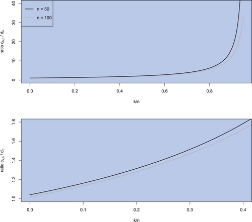
It is a well-known fact that the sample efficient frontier is overoptimistic and overestimates the location of the population efficient frontier in the mean–variance space (cf. Basak et al. 2005, Siegel and Woodgate 2007, Bodnar and Bodnar 2010). In contrast, the Bayesian approach provides an improved procedure which shrinks the sample efficient frontier by increasing the estimated variance of the global minimum portfolio and reducing the slope parameter. We will illustrate this point in Section 4 on real data described in Section 4.1.

3.3. Simulation study

We provide a detailed comparison of the estimators of the optimal portfolio weights, namely the suggested (objective) Bayesian approach, the estimator resulting from the (extended) Black–Litterman model, and the sample estimator, via simulations in this section. In the comparison study we also include two robust estimators of optimal portfolio weights (see, Chapter 20 in Würtz et al. 2015), which are based on the robust estimation of the mean vector and of the covariance matrix known as the minimum volume ellipsoid (MVE) estimator (see, e.g. Rousseeuw 1984) and the minimum covariance determinant (MCD) estimator (see, e.g. Rousseeuw and Driessen 1999). The aim of the Monte Carlo study is to assess the performance of each strategy in the estimation of the expected return and the variance of optimal portfolios. Such results will provide a better understanding about potential improvements which can be obtained by employing the new Bayesian approach.

The results of Proposition 4.6 of Bernardo and Smith (2000) ensure that the conditional multivariate normal distribution satisfies the imposed assumptions of infinitely exchangeability and of multivariate centred spherically symmetry. For that reason, we assume that the asset returns are independently and identically distributed given mean vector $\mathit{\mu }=({\mu }_1,\dots ,{\mu }_k{)}^{\mathrm{\top }}$ and covariance matrix $\mathbf{\Sigma }$ with the conditional distribution given by ${\mathbf{\text{X}}}_t|\mathit{\mu },\mathbf{\Sigma }\sim {\mathcal{N}}_k(\mathit{\mu },\mathbf{\Sigma })$. In order to avoid any restriction to specific values of $\mathit{\mu }$, the elements of this vector were generated from the uniform distribution on $[-0.01,0.01]$ in each simulation run, that is ${\mu }_i\sim Unif(-0.01,0.01)$. For the covariance matrix we consider its decomposition into the correlation matrix $\mathbf{\text{R}}$ and the diagonal matrix with standard deviations $\mathbf{\text{D}}=\mathrm{d}\mathrm{i}\mathrm{a}\mathrm{g}(d_1,\dots ,d_k)$, i.e. $\mathbf{\Sigma }=\mathbf{\text{DRD}}$. Two choices of volatility are considered: (i) low volatility with $d_i\sim Unif(0.002,0.005)$ and (ii) high volatility with $d_i\sim Unif(0.005,0.02)$. The correlation matrix is set to $\mathbf{\text{R}}=(1-\rho ){\mathbf{\text{I}}}_k+\rho {\mathbf{\text{J}}}_k$ with $\rho =0.6$, k-dimensional identity matrix ${\mathbf{\text{I}}}_k$, and the k-dimensional matrix of ones ${\mathbf{\text{J}}}_k$. We put $k\in \{5,10,25,40\}$, $n\in \{50,75,100,130\}$, and $\gamma =50$. In the case of the (extended) Black–Litterman model the precision parameters are $r_0=100$ and $d_0=100$, while ${\mathbf{\text{m}}}_0$ and ${\mathbf{\text{S}}}_0$ are obtained by perturbing $\mathit{\mu }$ and $\mathbf{\Sigma }$ as ${\mathbf{\text{m}}}_0=\mathit{\mu }+0.5\mathit{\epsilon }$ and ${\mathbf{\text{S}}}_0=\mathbf{\Sigma }+0.5\mathbf{\Delta }$ with $\mathit{\epsilon }=({\epsilon }_1,\dots {\epsilon }_k{)}^{\mathrm{\top }}$ and $\mathbf{\Delta }=diag({\delta }_1^2,\dots ,{\delta }_k^2)$ where ${\epsilon }_i\sim Unif(-0.01,0.01)$ and ${\delta }_i\sim Unif(0.001,0.005)$. The results in the tables are based on $B=10000$ independent repetitions.

As a measure of performance, the average absolute deviation from the resulting estimator to the corresponding true population value was computed for the portfolio expected return and the portfolio variance. The values are summarized in table 1 in the case of low volatilities and in table 2 for high volatilities. We observe that the application of the new objective Bayesian estimation strategy leads to the considerable improvements in terms of both performance measures meaning a better point estimation of both the portfolio expected return and the portfolio variance. The impact of the improvement increases as the portfolio dimension becomes larger. Especially, when k = 40 and n = 50 the new Bayesian estimator results in the values of the average deviation which are 12 times smaller than the one computed for the sample portfolio in the case of the portfolio expected return and about 11.7 times smaller in the case of the variance when the volatilities are low, while both these values are above 12.2 for high volatilities. These findings are in line with the results presented in figure 1. Also, a slightly better performance is observed in the case of the (extended) Black–Litterman estimation strategy when the portfolio dimension is large. In this case, it is ranked on the second place by using both criteria when k = 40 and n = 50, while it is on the third place in all other cases showing that the influence of the expert knowledge could have a great impact when the sample size is not large. Similar findings are also present for two robust portfolio selection strategies, which are ranked on the fourth and on the fifth places. Also, in these cases, the sample size is not large enough with respect to the portfolio dimension, which causes a bad performance of these two strategies. Finally, we point out that with the increase of the sample size, the values of the two performance measures becomes smaller and in the case of k = 5 and n = 130 they are almost the same for the new Bayesian approach and the sample method while the Bayesian approach is still more preferable.

Table 1. Average absolute deviation (AD) of the estimated portfolio expected return and of the estimated portfolio variance from their population values.

$\gamma =50$	AD of portfolio expected return				AD of portfolio variance
Bayesian
Black–Litterman
Sample	n = 50	n = 75	n = 100	n = 130	n = 50	n = 75	n = 100	n = 130
Robust, MVE
Robust, MCD
	0.1017	0.0822	0.0713	0.0621	0.0020	0.0016	0.0014	0.0012
	1.0889	0.7257	0.5438	0.4140	0.0218	0.0145	0.0109	0.0083
k = 5	0.1186	0.0912	0.0768	0.0660	0.0024	0.0018	0.0015	0.0013
	0.3824	0.2284	0.1751	0.1319	0.0076	0.0046	0.0035	0.0026
	0.2494	0.1984	0.1661	0.1459	0.0050	0.0040	0.0033	0.0029
	0.2541	0.1944	0.1660	0.1439	0.0051	0.0039	0.0033	0.0029
	2.6794	1.7051	1.2657	0.9547	0.0536	0.0341	0.0253	0.0191
k = 10	0.4127	0.2730	0.2183	0.1765	0.0083	0.0055	0.0044	0.0035
	1.0597	0.5949	0.4299	0.3305	0.0212	0.0119	0.0086	0.0066
	2.4460	0.9509	0.5799	0.3900	0.0489	0.0190	0.0116	0.0078
	0.8878	0.6205	0.5116	0.4236	0.0178	0.0124	0.0102	0.0085
	8.5916	4.8591	3.3871	2.4422	0.1718	0.0972	0.0677	0.0488
k = 25	3.9959	1.9720	1.3382	0.9466	0.0799	0.0394	0.0268	0.0189
	11.349	5.7082	3.3371	2.1340	0.2269	0.1142	0.0667	0.0427
	25.837	9.3763	5.2220	3.2756	0.5167	0.1875	0.1044	0.0655
	2.3320	1.2120	0.9153	0.7521	0.0466	0.0242	0.0183	0.0150
	16.5132	8.1638	5.1806	3.5884	0.3303	0.1633	0.1036	0.0718
k = 40	27.9857	7.4658	4.2657	2.8229	0.5597	0.1493	0.0853	0.0565
	73.6087	20.148	12.158	7.5067	1.4722	0.4030	0.2432	0.1501
	533.452	33.396	16.574	9.7837	10.669	0.6679	0.3315	0.1957

Notes: The smallest values are depicted in bold. Five considered estimators are the (objective) Bayesian estimator (first line in each panel), the estimator resulting from the (extended) Black–Litterman model (second line in each panel), the sample estimator (third line in each panel), the robust MVE estimator (fourth line in each panel), and the robust MCD estimator (fifth line in each panel) for several values of $k\in \{5,10,25,40\}$ and $n\in \{50,75,100,130\}$ with $\gamma =50$. The asset returns are assumed to be conditionally normally distributed with small variances.

Table 2. Average absolute deviation (AD) of the estimated portfolio expected return and of the estimated portfolio variance from their population values.

$\gamma =50$	AD of portfolio expected return				AD of portfolio variance
Bayesian
Black–Litterman
Sample	n = 50	n = 75	n = 100	n = 130	n = 50	n = 75	n = 100	n = 130
Robust, MVE
Robust, MCD
	0.0111	0.0091	0.0079	0.0070	0.0002	0.0002	0.0002	0.0001
	0.0932	0.0629	0.0473	0.0361	0.0018	0.0012	0.0009	0.0007
k = 5	0.0133	0.0102	0.0086	0.0075	0.0003	0.0002	0.0002	0.0001
	0.0292	0.0192	0.0154	0.0123	0.0006	0.0004	0.0003	0.0002
	0.0389	0.0234	0.0177	0.0132	0.0008	0.0005	0.0003	0.0003
	0.0256	0.0200	0.0171	0.0147	0.0005	0.0004	0.0003	0.0003
	0.2397	0.1542	0.1155	0.0874	0.0048	0.0031	0.0023	0.0017
k = 10	0.0431	0.0287	0.0229	0.0184	0.0009	0.0006	0.0005	0.0004
	0.1079	0.0600	0.0435	0.0331	0.0021	0.0012	0.0009	0.0007
	0.2498	0.0956	0.0584	0.0390	0.0050	0.0019	0.0012	0.0008
	0.0878	0.0619	0.0512	0.0428	0.0018	0.0012	0.0010	0.0009
	0.7786	0.4504	0.3171	0.2310	0.0156	0.0090	0.0063	0.0046
k = 25	0.4062	0.2003	0.1355	0.0966	0.0081	0.0040	0.0027	0.0019
	1.1483	0.5773	0.3361	0.2148	0.0230	0.0115	0.0067	0.0043
	2.6215	0.9502	0.5253	0.3290	0.0524	0.0190	0.0105	0.0066
	0.2280	0.1200	0.0915	0.0747	0.0046	0.0024	0.0018	0.0015
	1.4380	0.7473	0.4825	0.3379	0.0288	0.0149	0.0096	0.0068
k = 40	2.8277	0.7556	0.4309	0.2848	0.0565	0.0151	0.0086	0.0057
	7.3905	2.0316	1.2234	0.7575	0.1478	0.0406	0.0245	0.0151
	52.933	3.3593	1.6674	0.9872	1.0587	0.0672	0.0333	0.0197

Notes: The smallest values are depicted in bold. The five estimators are the (objective) Bayesian estimator (first line in each panel), the estimator resulting from the (extended) Black–Litterman model (second line in each panel), the sample estimator (third line in each panel), the robust MVE estimator (fourth line in each panel), and the robust MCD estimator (fifth line in each panel) for several values of $k\in \{5,10,25,40\}$ and $n\in \{50,75,100,130\}$ with $\gamma =50$. The asset returns are assumed to be conditionally normally distributed with large variances.

3.4. Robustness analysis

Next, we investigate how robust are the numerical findings obtained in the previous section to the deviation from the conditional normality. For this purposed, we employ the conditional multivariate t-distribution with 5 degrees of freedom, which has the same mean vector $\mathit{\mu }$ and the same covariance matrices $\mathbf{\Sigma }$ as in the case of the model from Section 3.3. Furthermore, it is noted that in contrast to the conditional multivariate normal distribution, the conditional multivariate t-distribution does not belong to the family of infinitely exchangeability and multivariate centred spherically symmetrical distributions.

The replacement of the conditional multivariate normal distribution by the conditional multivariate t-distribution influences the values of the average absolute deviation computed in both cases of the portfolio expected return and of the portfolio variance. All these values become considerably larger which is explained by the heavy-tailed nature of the multivariate t-distribution (see tables 3 and 4). On the other side, the ranking between the five estimation strategies does not change. The new (objective) Bayesian approach outperforms the other four competitors in all of the considered cases similarly when the observation data were generated from the multivariate normal distribution. Also, in the case of the large-dimensional portfolio consisting of 40 assets and the sample size equal to n = 50, the (extended) Black–Litterman approach is ranked on the second place for both low and high volatilities, while the sample estimator performs better in the rest of the considered cases.

Table 3. Average absolute deviation (AD) of the estimated portfolio expected return and of the estimated portfolio variance from their population values.

$\gamma =50$	AD of portfolio expected return				AD of portfolio variance
Bayesian
Black–Litterman
Sample	n = 50	n = 75	n = 100	n = 130	n = 50	n = 75	n = 100	n = 130
Robust, MVE
Robust, MCD
	0.1490	0.1209	0.1088	0.0956	0.0030	0.0024	0.0022	0.0019
	1.2668	0.8216	0.6116	0.4632	0.0253	0.0164	0.0122	0.0093
k = 5	0.1971	0.1480	0.1268	0.1076	0.0039	0.0030	0.0025	0.0022
	0.7206	0.5815	0.5211	0.4857	0.0144	0.0116	0.0104	0.0097
	0.7974	0.6005	0.5240	0.4836	0.0159	0.0120	0.0105	0.0097
	0.3728	0.3008	0.2633	0.2272	0.0075	0.0060	0.0053	0.0045
	3.3112	2.0669	1.5232	1.1441	0.0662	0.0413	0.0305	0.0229
k = 10	0.7125	0.4794	0.3833	0.3089	0.0143	0.0096	0.0077	0.0062
	2.3178	1.6962	1.4892	1.3501	0.0464	0.0339	0.0298	0.0270
	3.6668	2.1039	1.6832	1.4458	0.0733	0.0421	0.0337	0.0289
	1.4528	1.1011	0.9058	0.7880	0.0291	0.0220	0.0181	0.0158
	11.873	6.8656	4.7531	3.4785	0.2374	0.1373	0.0951	0.0696
k = 25	6.8816	3.5138	2.3958	1.7749	0.1376	0.0703	0.0479	0.0355
	18.522	10.176	7.0974	5.6988	0.3704	0.2035	0.1419	0.1140
	29.560	14.142	10.194	8.1919	0.5912	0.2828	0.2039	0.1638
	3.2387	2.3571	1.9424	1.6140	0.0648	0.0471	0.0388	0.0323
	22.5595	12.4591	8.3420	5.9158	0.4512	0.2492	0.1668	0.1183
k = 40	46.3159	12.7395	7.5904	5.1566	0.9263	0.2548	0.1518	0.1031
	117.427	33.2640	20.775	14.454	2.3485	0.6653	0.4155	0.2891
	541.115	42.8432	25.721	18.805	10.822	0.8569	0.5144	0.3761

Notes: The smallest values are depicted in bold. The five estimators are the (objective) Bayesian estimator (first line in each panel), the estimator resulting from the (extended) Black–Litterman model (second line in each panel), the sample estimator (third line in each panel), the robust MVE estimator (fourth line in each panel), and the robust MCD estimator (fifth line in each panel) for several values of $k\in \{5,10,25,40\}$ and $n\in \{50,75,100,130\}$ with $\gamma =50$. The asset returns are assumed to be conditionally multivariate t-distributed with 5 degrees of freedom and small variances.

Table 4. Average absolute deviation (AD) of the estimated portfolio expected return and of the estimated portfolio variance from their population values.

$\gamma =50$	AD of portfolio expected return				AD of portfolio variance
Bayesian
Black–Litterman
Sample	n = 50	n = 75	n = 100	n = 130	n = 50	n = 75	n = 100	n = 130
Robust, MVE
Robust, MCD
	0.0150	0.0123	0.0110	0.0096	0.0003	0.0002	0.0002	0.0002
	0.1085	0.0710	0.0533	0.0405	0.0021	0.0014	0.0010	0.0008
k = 5	0.0196	0.0149	0.0127	0.0107	0.0004	0.0003	0.0003	0.0002
	0.0671	0.0528	0.0472	0.0436	0.0013	0.0010	0.0009	0.0009
	0.0737	0.0544	0.0475	0.0435	0.0014	0.0011	0.0009	0.0008
	0.0374	0.0300	0.0263	0.0225	0.0007	0.0006	0.0005	0.0004
	0.2958	0.1863	0.1386	0.1043	0.0059	0.0037	0.0028	0.0021
k = 10	0.0706	0.0474	0.0379	0.0303	0.0014	0.0009	0.0008	0.0006
	0.2242	0.1613	0.1412	0.1271	0.0045	0.0032	0.0028	0.0025
	0.3534	0.1998	0.1592	0.1361	0.0070	0.0040	0.0032	0.0027
	0.1476	0.1116	0.0912	0.0792	0.0023	0.0022	0.0018	0.0015
	1.0651	0.6335	0.4441	0.3277	0.0213	0.0127	0.0089	0.0065
k = 25	0.6878	0.3502	0.2383	0.1763	0.0137	0.0070	0.0048	0.0035
	1.8374	1.0074	0.6999	0.5614	0.0367	0.0201	0.0140	0.0112
	2.9172	1.3960	1.0026	0.8062	0.0583	0.0279	0.0200	0.0161
	0.3257	0.2392	0.1970	0.1630	0.0065	0.0048	0.0039	0.0033
	1.9528	1.1312	0.7753	0.5575	0.0391	0.0226	0.0155	0.0111
k = 40	4.6225	1.2720	0.7580	0.5142	0.0924	0.0254	0.0152	0.0103
	11.768	3.3082	2.0689	1.4391	0.2354	0.0662	0.0414	0.0288
	49.947	4.2723	2.5567	1.8670	0.9989	0.0854	0.0511	0.0373

Notes: The smallest values are depicted in bold. The five estimators are the (objective) Bayesian estimator (first line in each panel), the estimator resulting from the (extended) Black–Litterman model (second line in each panel), the sample estimator (third line in each panel), the robust MVE estimator (fourth line in each panel), and the robust MCD estimator (fifth line in each panel) for several values of $k\in \{5,10,25,40\}$ and $n\in \{50,75,100,130\}$ with $\gamma =50$. The asset returns are assumed to be conditionally multivariate t-distributed with 5 degrees of freedom and large variances.

4. Empirical illustration

4.1. Data

For the first empirical illustration, we use weekly returns from a collection of assets of the S&P500, allowing for portfolios ranging from 5 to 40 assets. A similar setup is also used in the second empirical illustration where monthly returns instead of weekly returns are used. The parameters are estimated with sample sizes of $n\in \{52,78,104,130\}$, corresponding to one year up to two and a half years of weekly data or to approximately four and a half up to eleven years of monthly data. All the data end on the 8th of October 2017. The constructed portfolios consist of $k\in \{5,10,25,40\}$ assets. The hyperparameters in the extended Black–Litterman model are obtained by employing the empirical Bayes approach (see, e.g. Gelman et al. 2014, Bauder et al. 2020). This allows us to analyse the behaviour of the proposed model not only in terms of economic risk but also regarding statistical estimation uncertainty.

4.2. Results for weekly data

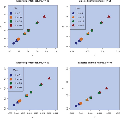
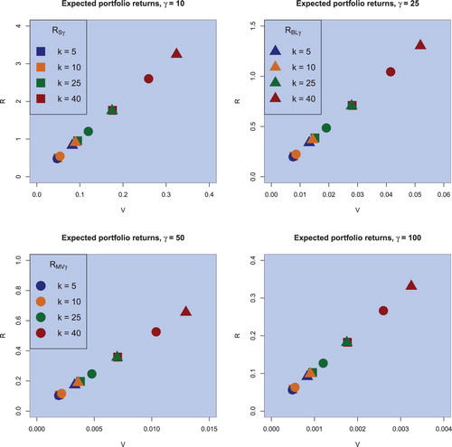
As mentioned in Section 3, there is a distinct difference between the classical sample estimators and the (objective) Bayesian estimators proposed in this paper. With this conclusion and the fact that the sample efficient frontier overestimates the population efficient frontier, we expect the estimators for the expected return and the variance to be larger in the Bayesian case compared to the sample estimators indicating that the (objective) Bayesian approach also takes the estimation risk into account in its construction which in practice automatically leads to smaller values of the risk aversion coefficient in comparison to the conventional case. Figure 2 illustrates this presumption: fixing n = 130 and considering different portfolio sizes $k\in \{5,10,25,40\}$ for different risk attitudes $\gamma \in \{10,25,50,100\}$, we find that for the same value of the risk coefficient γ and for the same portfolio size, the (objective) Bayesian estimator performs as expected compared to the sample estimator, whereas the Black–Litterman optimal portfolios exhibit a more exaggerated behaviour. The latter results are related to the usage of the additional information in the construction of the Black–Litterman optimal portfolios which, in particular, can lead to the increase of uncertainty especially when the hyperparameters differ considerably from the corresponding population values as shown in the simulation study of Section 3. Furthermore, the difference in the estimators increases if the number of assets gets closer to the sample size, as illustrated in figure 1 or when γ decreases, i.e. for less risk averse investors the impact of parameter uncertainty becomes larger.

Figure 2. Sample optimal portfolios (squares), (objective) Bayesian optimal portfolios (circles), and the Black–Litterman optimal portfolios (triangulares) for the risk aversion coefficient of $\gamma \in \{10,25,50,100\}$, for the sample case of n = 130 and for the portfolio dimension of $k\in \{5,10,25,40\}$ in the case of weekly data.

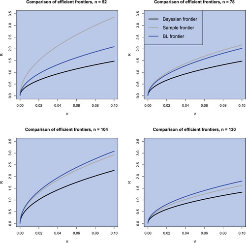
Regarding the efficient frontier, figure 3 shows the estimated efficient frontiers for a fixed sample size of n = 130 and varying portfolio sizes $k\in \{5,10,25,40\}$ in all three cases, namely the sample efficient frontier, the (objective) Bayesian efficient frontier, and the Black–Litterman efficient frontier. The (objective) Bayesian efficient frontier lies always below the sample efficient frontier and therefore exhibits less overestimation of the population efficient frontier. In contrast, the Black–Litterman frontier exhibits even a stronger overestimation compared to the population efficient frontier due to the uncertainty related to hyperparameters which are present in the model. Furthermore, figure 3 also illustrates the finding shown in figure 1. The estimators of the efficient frontier deviate stronger when the portfolio size gets closer to the sample size. This fact is also illustrated in figure 4 for fixed k = 40 and varying $n\in \{52,78,104,130\}$. 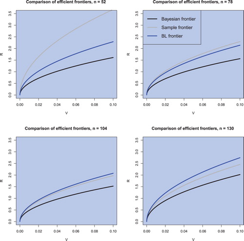The (objective) Bayesian and the sample estimated efficient frontiers coincide more the larger the sample size n is, whereas the Black–Litterman efficient frontier appears to exhibit stronger overestimation with growing sample size. This is in line with the theoretical implications. Finally, we also observe the increase in the slope parameter of the efficient frontier when the portfolio dimension increases indicating the well-documented positive effect of portfolio diversification.

Figure 3. The sample efficient frontier, the (objective) Bayesian efficient frontier, and the Black–Litterman efficient frontier for n = 130 and $k\in \{5,10,25,40\}$ in the case of weekly data.

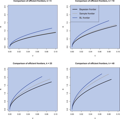
Figure 4. The sample efficient frontier, the (objective) Bayesian efficient frontier, and the Black–Litterman efficient frontier for k = 40 and $n\in \{52,78,104,130\}$ in the case of weekly data.

4.3. Results for monthly data

Figure 5 shows the location of the sample optimal portfolios, of the (objective) Bayesian optimal portfolios, and of the Black–Litterman optimal portfolios computed for the same values of the risk aversion coefficient γ, portfolio dimension k, and sample size n as in figure 2 in the case of monthly data. The distinct difference between the classical sample estimators, the (objective) Bayesian estimators, and the Black–Litterman optimal portfolios is also identified for monthly data. In contrast to figure 2 we observe a considerable reduction in both the expected returns and the variances of all constructed optimal portfolios, while their ordering with respect to the location in the mean–variance space is the same as the one observed in figure 2. For the same value of the investor risk aversion coefficient the sample optimal portfolios exhibit smaller values of the expected return and the variance following by the (objective) Bayesian optimal portfolio which incorporate the parameter uncertainty into account in their construction. Finally, the uncertainty about the hyperparameters move the Black–Litterman optimal portfolios futher in the direction of larger values of the expected return and variance.

Figure 5. Sample optimal portfolios (squares), (objective) Bayesian optimal portfolios (circles), and the Black–Litterman optimal portfolios (triangulares) for the risk aversion coefficient of $\gamma \in \{10,25,50,100\}$, for the sample case of n = 130 and for the portfolio dimension of $k\in \{5,10,25,40\}$ in the case of monthly data.

Similar findings are also present in figures 6 and 7 where the sample efficient frontier, the (objective) Bayesian efficient frontier, and the Black–Litterman efficient frontier are drawn for several values of portfolio dimension k and sample size n. Both the sample efficient frontier and the Black–Litterman efficient frontier lie above the (objective) Bayesian efficient frontier tending to provide a considerable overestimation of the population efficient frontier especially when the portfolio dimension is large in comparison to the sample size. In figure 7 we also observe that sample efficient frontier is located above the other two estimators when the sample size is only slightly larger than portfolio dimension k = 40 indicating its poor performance in such situations independently of the data frequency used in the estimation. On the other side, the Black–Litterman efficient frontier demonstrates its dependence on the chosen hyperparameters used in its construction. The considerable sample sizes in both figures 6 and 7 seem to be not large enough to reduce the effect of the hyperparameters on the resulting estimator of the efficient frontier. Better results are expected for larger sample sizes following the Bernstein–von Mises theorem (cf. Bernardo and Smith 2000).

Figure 6. The sample efficient frontier, the (objective) Bayesian efficient frontier, and the Black–Litterman efficient frontier for n = 130 and $k\in \{5,10,25,40\}$ in the case of monthly data.

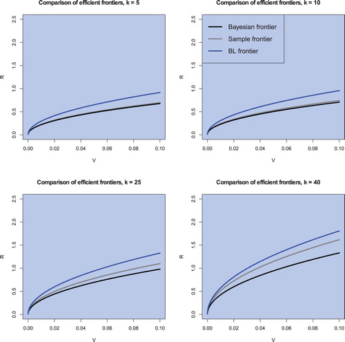
Figure 7. The sample efficient frontier, the (objective) Bayesian efficient frontier, and the Black–Litterman efficient frontier for k = 40 and $n\in \{52,78,104,130\}$ in the case of monthly data.

4.4. Posterior interval prediction

In contrast to the conventional procedure, both the (objective) Bayesian approach and the application of the Black–Litterman model provide also the whole posterior predictive distribution of the optimal portfolio return and not only the point estimator of its weights. Using data described in Section 4.1, we calculate in this section the prediction intervals for the optimal portfolio returns for several values of the risk-aversion coefficient $\gamma \in \{10,20,\dots ,100\}$, for $k\in \{5,25\}$, and for $n\in \{52,78,104,130\}$ in the case of weekly data (see, figures 8 for the (objective) Bayesian approach and 9 for the Black–Litterman model) and in the case of monthly data (see, figures 10 for the (objective) Bayesian approach and figure 11 for the Black–Litterman model).

Figure 8. Credible intervals for the return of optimal portfolios with varying risk attitudes for weekly data obtained by employing the (objective) Bayesian approach. The sample sizes are chosen to be $n\in \{52,78,104,130\}$ and the portfolio dimension is fixed to k = 25. The confidence level is set to $\alpha =0.05$.

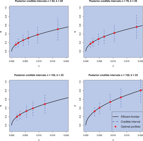
Figure 9. Credible intervals for the return of optimal portfolios for the Black–Litterman model with varying risk attitudes for weekly data. The sample sizes are chosen to be $n\in \{52,78,104,130\}$ and the portfolio dimension is fixed to k = 25. The confidence level is set to $\alpha =0.05$.

Figure 10. Credible intervals for the return of optimal portfolios with varying risk attitudes for monthly data obtained by employing the (objective) Bayesian approach. The sample sizes are chosen to be $n\in \{52,78,104,130\}$ and the portfolio dimension is fixed to k = 25. The confidence level is set to $\alpha =0.05$.

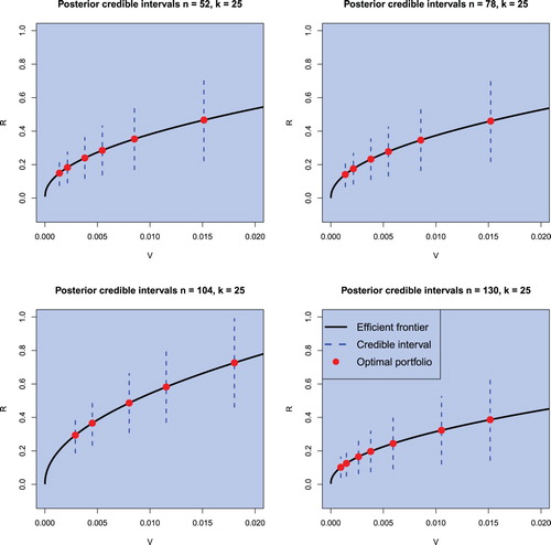
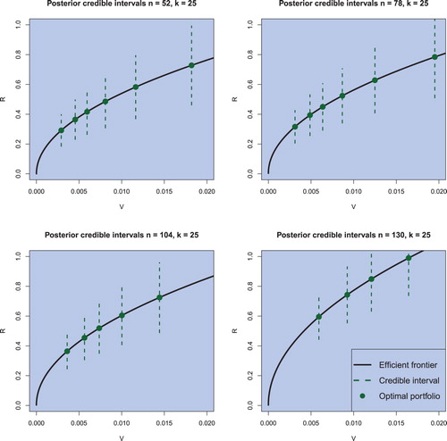
Figure 11. Credible intervals for the return of optimal portfolios for the Black–Litterman model with varying risk attitudes for monthly data. The sample sizes are chosen to be $n\in \{52,78,104,130\}$ and the portfolio dimension is fixed to k = 25. The confidence level is set to $\alpha =0.05$.

The prediction intervals in figures 8 – 11 are obtained by using the following procedure:

1. Fix γ and calculate the expected return and the variance of the corresponding mean–variance optimal portfolio as given (9(9) $R_{MV,\gamma }=\frac{{\mathbf{\text{1}}}^{\mathrm{\top }}{\mathbf{\text{S}}}_{t-1}^{-1}{\overline{\mathbf{\text{x}}}}_{t-1}}{{\mathbf{\text{1}}}^{\mathrm{\prime }}{\mathbf{\text{S}}}_{t-1}^{-1}\mathbf{\text{1}}}+{\gamma }^{-1}{c}_{k,n}^{-1}{\overline{\mathbf{\text{x}}}}_{t-1}^{\mathrm{\top }}{\mathbf{\text{Q}}}_{t-1}{\overline{\mathbf{\text{x}}}}_{t-1}$(9) ) and (10(10) $V_{MV,\gamma }=\frac{c_{k,n}}{{\mathbf{\text{1}}}^{\mathrm{\prime }}{\mathbf{\text{S}}}_{t-1}^{-1}\mathbf{\text{1}}}+{\gamma }^{-2}{c}_{k,n}^{-1}{\overline{\mathbf{\text{x}}}}_{t-1}^{\mathrm{\top }}{\mathbf{\text{Q}}}_{t-1}{\overline{\mathbf{\text{x}}}}_{t-1},$(10) ) for the (objective) Bayesian approach and in (22(22) $R_{MV,\gamma }=\frac{{\mathbf{\text{1}}}^{\mathrm{\top }}{\mathbf{\text{S}}}_{t-1,I}^{-1}{\overline{\mathbf{\text{x}}}}_{t-1,I}}{{\mathbf{\text{1}}}^{\mathrm{\prime }}{\mathbf{\text{S}}}_{t-1,I}^{-1}\mathbf{\text{1}}}+{\gamma }^{-1}{q}_{k,n}^{-1}{\overline{\mathbf{\text{x}}}}_{t-1,I}^{\mathrm{\top }}{\mathbf{\text{Q}}}_{t-1,I}{\overline{\mathbf{\text{x}}}}_{t-1,I}$(22) ) and (23(23) $V_{MV,\gamma }=\frac{q_{k,n}}{{\mathbf{\text{1}}}^{\mathrm{\prime }}{\mathbf{\text{S}}}_{t-1,I}^{-1}\mathbf{\text{1}}}+{\gamma }^{-2}{q}_{k,n}^{-1}{\overline{\mathbf{\text{x}}}}_{t-1,I}^{\mathrm{\top }}{\mathbf{\text{Q}}}_{t-1,I}{\overline{\mathbf{\text{x}}}}_{t-1,I}.$(23) ) for the Black–Litterman model;

2. For chosen γ, compute the weights of the optimal mean–variance portfolio ${\mathbf{\text{w}}}_{MV,\gamma }$ using (8(8) $\begin{array}{rl}{\mathbf{\text{w}}}_{MV,\gamma }& =\frac{{\mathbf{\text{S}}}_{t-1}^{-1}\mathbf{\text{1}}}{{\mathbf{\text{1}}}^{\mathrm{\prime }}{\mathbf{\text{S}}}_{t-1}^{-1}\mathbf{\text{1}}}+{\gamma }^{-1}{c}_{k,n}^{-1}{\mathbf{\text{Q}}}_{t-1}{\overline{\mathbf{\text{x}}}}_{t-1}\mathrm{w}\mathrm{i}\mathrm{t}\mathrm{h}\\ {\mathbf{\text{Q}}}_{t-1}& ={\mathbf{\text{S}}}_{t-1}^{-1}-\frac{{\mathbf{\text{S}}}_{t-1}^{-1}\mathbf{\text{1}}{\mathbf{\text{1}}}^{\mathrm{\prime }}{\mathbf{\text{S}}}_{t-1}^{-1}}{{\mathbf{\text{1}}}^{\mathrm{\prime }}{\mathbf{\text{S}}}_{t-1}^{-1}\mathbf{\text{1}}}\end{array}$(8) ) for the (objective) Bayesian approach and (21(21) $\begin{array}{rl}{\mathbf{\text{w}}}_{MV,\gamma }& =\frac{{\mathbf{\text{S}}}_{t-1,I}^{-1}\mathbf{\text{1}}}{{\mathbf{\text{1}}}^{\mathrm{\prime }}{\mathbf{\text{S}}}_{t-1,I}^{-1}\mathbf{\text{1}}}+{\gamma }^{-1}{q}_{k,n}^{-1}{\mathbf{\text{Q}}}_{t-1,I}{\overline{\mathbf{\text{x}}}}_{t-1,I}\mathrm{w}\mathrm{i}\mathrm{t}\mathrm{h}\\ {\mathbf{\text{Q}}}_{t-1,I}& ={\mathbf{\text{S}}}_{t-1,I}^{-1}-\frac{{\mathbf{\text{S}}}_{t-1,I}^{-1}\mathbf{\text{1}}{\mathbf{\text{1}}}^{\mathrm{\prime }}{\mathbf{\text{S}}}_{t-1,I}^{-1}}{{\mathbf{\text{1}}}^{\mathrm{\prime }}{\mathbf{\text{S}}}_{t-1,I}^{-1}\mathbf{\text{1}}}\end{array}$(21) ) for the Black–Litterman model;

3. In using ${\mathbf{\text{w}}}_{MV,\gamma }$ apply the results of Theorem 1 and Algorithm 1 for the (objective) Bayesian approach and Theorem 2 and Algorithm 2 for the Black–Litterman model to get a sample of optimal portfolio returns denoted by $R_{MV,\gamma }^{\left(b\right)}$ for $b=1,\dots ,B$;

4. Fix the significance level of the prediction interval α and compute the $\alpha /2$- and $(1-\alpha /2)$- quantiles from the empirical distribution of $R_{MV,\gamma }^{\left(b\right)}$, $b=1,\dots ,B$ in both cases of the (objective) Bayesian approach and of the Black–Litterman model;

5. For the computed value of $V_{MV,\gamma }$ in part (a), plot the point prediction $R_{MV,\gamma }$ from (a) together with the prediction interval from (d). This procedure is performed separately for the sample $R_{MV,\gamma }^{\left(b\right)}$ for $b=1,\dots ,B$ obtained by employing the (objective) Bayesian approach and for a similar sample obtained by using the Black–Litterman model.

The order of the efficient portfolios given in figures 8– 11 is directly determined by the risk aversion coefficient. The smaller γ, the riskier is the portfolio and lies therefore more right on the efficient frontier. We observe that the optimal efficient portfolios are shifted to the right for growing sample sizes. But the focus lies here on the credible intervals for a confidence level of $\alpha =0.05$. The first observation is that no credible interval covers negative values, implying positive portfolio returns with probability of $95\mathrm{\%}$. The second observation is that the credible intervals become larger the more risky an efficient portfolio becomes—which is in line with the theory. And the third observation is that these credible intervals for riskier efficient portfolios become larger regardless of the increased sample size. Hence, the decrease in estimation risk resulting from a larger sample is outweighed by the economic risk.

As in the previous section, no differences between the results obtained by using weekly data or monthly data are detected. Most noteworthy is the case of n = 130 for monthly data as shown in figures 10 and 11, covering the financial crisis of 2008, showing a drastic drop in returns compared to different periods but also exhibiting credible intervals which do not cover negative values. To this end, we note that the optimal Black–Litterman portfolios are located further on the efficient frontier in comparison to the (objective) Bayesian optimal portfolio computed for the same value of the risk aversion coefficient and they also have larger prediction intervals indicating larger amount of uncertainty which is present when the optimal Black–Litterman portfolios are constructed.

5. Conclusion

The mean–variance analysis of Markowitz presents a fundamental method of portfolio construction which is very popular in the financial literature today. It provides an investor with the portfolio weights which determine the structure of the optimal portfolio. However, the investor faces a number of difficulties in implementing this procedure in practice. One of the main pitfalls of the mean–variance analysis is that its solution is presented in terms of unobservable quantities, the parameters of the asset returns distribution. As a result, the optimization problem is performed in two steps. After finding the analytical solution, the optimal portfolio is constructed by replacing the unknown parameters with their estimates. Due to the considerable influence of parameter uncertainty on the investment process, this procedure leads only to sub-optimal portfolios.

We deal with the problem from the viewpoint of Bayesian statistics. The optimization problem is formulated in terms of the posterior predictive distribution which does not involve unknown quantities. Consequently, we deal with parameter uncertainty before solving the optimization problem. This approach allows us to find optimal portfolio weights which now depend only on historical observations of the asset returns. The advantages of the approach are shown both theoretically and empirically. In particular, we show that the constructed Bayesian efficient frontier improves on the overoptimism present in the sample efficient frontier. Another important advantage of the suggested procedure is that it allows us not only to construct an optimal portfolio based on the posterior predictive distribution, but also leads to an intelligent technique by performing an interval forecast of future realizations of optimal portfolio returns which are obtained by employing the derived stochastic representation of the posterior predictive distribution.

Acknowledgments

The authors would like to thank Professor Michael Dempster, Professor Jim Gatheral and two anonymous Reviewers for their helpful suggestions. This research was partly supported by the German Science Foundation (DFG) via the projects BO 3521/3-1 and SCHM 859/13-1 ‘Bayesian Estimation of the Multi-Period Optimal Portfolio Weights and Risk Measures’ and by the Swedish Research Council (VR) via the project ‘Bayesian Analysis of Optimal Portfolios and Their Risk Measures’.

Disclosure statement

No potential conflict of interest was reported by the author(s).

ORCID

Nestor Parolya  http://orcid.org/0000-0003-2147-2288

Additional information

Funding

This research was partly supported by the German Science Foundation (DFG) via the projects BO 3521/3-1 and SCHM 859/13-1 ‘Bayesian Estimation of the Multi-Period Optimal Portfolio Weights and Risk Measures’ and by the Swedish Research Council (VR) via the project ‘Bayesian Analysis of Optimal Portfolios and Their Risk Measures’.

Appendix

Proof of Theorem 1.

Proof of Theorem 1

The assumptions of infinitely exchangeability and multivariate centred spherically symmetry implies (see, e.g. Bernardo and Smith 2000, Proposition 4.6) that the asset returns are independently and identically distributed given the mean vector $\mathit{\mu }$ and the covariance matrix $\mathbf{\Sigma }$ with the conditional distribution given by ${\mathbf{\text{X}}}_t|\mathit{\mu },\mathbf{\Sigma }\sim {\mathcal{N}}_k(\mathit{\mu },\mathbf{\Sigma })$ (k-dimensional normal distribution with mean vector $\mathit{\mu }$ and covariance matrix $\mathbf{\Sigma }$). Under this model with $\mathit{\theta }=(\mathit{\mu },\mathbf{\Sigma })$, Jeffreys' prior is given by (A1) $\pi (\mathit{\mu },\mathbf{\Sigma })\propto |\mathbf{\Sigma }{|}^{-(k+1)/2},$(A1) which leads to the posterior expressed as (A2) $\begin{array}{rl}\pi (\mathit{\mu },\mathbf{\Sigma }|{\mathbf{\text{x}}}_{(t-1)})& \propto |\mathbf{\Sigma }{|}^{-(n+k+1)/2}\exp \left\{-\frac{n}{2}({\overline{\mathbf{\text{x}}}}_{t-1}-\mathit{\mu }{)}^{\mathrm{\top }}\right.\\ & \left.\times {\mathbf{\Sigma }}^{-1}({\overline{\mathbf{\text{x}}}}_{t-1}-\mathit{\mu })-\frac{1}{2}\mathrm{t}\mathrm{r}\left[{\mathbf{\text{S}}}_{t-1}{\mathbf{\Sigma }}^{-1}\right]\right\},\end{array}$(A2) where ${\overline{\mathbf{\text{x}}}}_{t-1}$ and ${\mathbf{\text{S}}}_{t-1}$ are given in the statement of the theorem.

From (A2(A2) $\begin{array}{rl}\pi (\mathit{\mu },\mathbf{\Sigma }|{\mathbf{\text{x}}}_{(t-1)})& \propto |\mathbf{\Sigma }{|}^{-(n+k+1)/2}\exp \left\{-\frac{n}{2}({\overline{\mathbf{\text{x}}}}_{t-1}-\mathit{\mu }{)}^{\mathrm{\top }}\right.\\ & \left.\times {\mathbf{\Sigma }}^{-1}({\overline{\mathbf{\text{x}}}}_{t-1}-\mathit{\mu })-\frac{1}{2}\mathrm{t}\mathrm{r}\left[{\mathbf{\text{S}}}_{t-1}{\mathbf{\Sigma }}^{-1}\right]\right\},\end{array}$(A2) ) we obtain that the posterior distribution of $\mathbf{\Sigma }$ is the inverse Wishart distribution (see Gupta and Nagar 2000 for the definition and properties) given by (A3) $\begin{array}{rl}& \mathbf{\Sigma }|\mathit{\mu },{\mathbf{\text{x}}}_{t-1}\sim {\mathcal{I}\mathcal{W}}_k(n+k+1,{\widetilde{\mathbf{\text{S}}}}_{t-1}(\mathit{\mu }\left)\right)\mathrm{w}\mathrm{i}\mathrm{t}\mathrm{h}\\ & {\widetilde{\mathbf{\text{S}}}}_{t-1}\left(\mathit{\mu }\right)={\mathbf{\text{S}}}_{t-1}+n(\mathit{\mu }-{\overline{\mathbf{\text{x}}}}_{t-1})(\mathit{\mu }-{\overline{\mathbf{\text{x}}}}_{t-1}{)}^{\mathrm{\top }}.\end{array}$(A3) Furthermore, integrating out $\mathbf{\Sigma }$ we get the marginal posterior for $\mathit{\mu }$ expressed as $\begin{array}{rl}\pi \left(\mathit{\mu }|{\mathbf{\text{x}}}_{(t-1)}\right)& \propto {\int }_{\mathbf{\Sigma }>0}|\mathbf{\Sigma }{|}^{-(n+k+1)/2}\exp \left\{-\frac{1}{2}\mathrm{t}\mathrm{r}\right.\\ & \left.\times \left[\left(n\right({\overline{\mathbf{\text{x}}}}_{t-1}-\mathit{\mu }\left)\right({\overline{\mathbf{\text{x}}}}_{t-1}-\mathit{\mu }{)}^{\mathrm{\top }}+{\mathbf{\text{S}}}_{t-1}){\mathbf{\Sigma }}^{-1}\right]\right\}\mathrm{d}\mathbf{\Sigma }\\ & \propto |n({\overline{\mathbf{\text{x}}}}_{t-1}-\mathit{\mu })({\overline{\mathbf{\text{x}}}}_{t-1}-\mathit{\mu }{)}^{\mathrm{\top }}+{\mathbf{\text{S}}}_{t-1}{|}^{-n/2},\end{array}$ where the last equality follows by observing that the function under the integral is the density function of the inverse Wishart distribution with n + k + 1 degrees of freedom and parameter matrix $n({\overline{\mathbf{\text{x}}}}_{t-1}-\mathit{\mu })({\overline{\mathbf{\text{x}}}}_{t-1}-\mathit{\mu }{)}^{\mathrm{\top }}+{\mathbf{\text{S}}}_{t-1}$. The application of Silvester's determinant theorem leads to (A4) $\pi \left(\mathit{\mu }|{\mathbf{\text{x}}}_{(t-1)}\right)\propto {\left(1+n({\overline{\mathbf{\text{x}}}}_{t-1}-\mathit{\mu }{)}^{\mathrm{\top }}{\mathbf{\text{S}}}_{t-1}^{-1}({\overline{\mathbf{\text{x}}}}_{t-1}-\mathit{\mu })\right)}^{-n/2},$(A4) which proves that $\mathit{\mu }|{\mathbf{\text{x}}}_{t-1}\sim t_k(n-k,{\overline{\mathbf{\text{x}}}}_{t-1},(1/n(n-k)\left){\mathbf{\text{S}}}_{t-1}\right)$ (k-dimensional multivariate t-distribution with n−k degrees of freedom, location vector ${\overline{\mathbf{\text{x}}}}_{t-1}$, and scale matrix $\left(1/n(n-k)\right){\mathbf{\text{S}}}_{t-1}$).

Because ${\mathbf{\text{X}}}_{t-n},\dots ,{\mathbf{\text{X}}}_t$ are independent given $\mathit{\mu }$ and $\mathbf{\Sigma }$ as well as conditionally normally distributed, we get that the conditional distribution $X_{p,t}|\mathit{\mu },\mathbf{\Sigma }$ coincides with $X_{p,t}|\mathit{\mu },\mathbf{\Sigma },{\mathbf{\text{x}}}_{(t-1)}$ is given by $X_{p,t}|\mathit{\mu },\mathbf{\Sigma },{\mathbf{\text{x}}}_{(t-1)}\sim \mathcal{N}({\mathbf{\text{w}}}^{\mathrm{\top }}\mathit{\mu },{\mathbf{\text{w}}}^{\mathrm{\top }}\mathbf{\Sigma }\mathbf{\text{w}}),$ where the last equality proves that $X_{p,t}$ depends on $\mathit{\mu }$, $\mathbf{\Sigma }$, and ${\mathbf{\text{x}}}_{(t-1)}$ only over ${\mathbf{\text{w}}}^{\mathrm{\top }}\mathit{\mu }$ and ${\mathbf{\text{w}}}^{\mathrm{\top }}\mathbf{\Sigma }\mathbf{\text{w}}$.

The application of Theorem 3.2.13 in Muirhead (1982) leads to (A5) $\frac{{\mathbf{\text{w}}}^{\mathrm{\top }}\mathbf{\Sigma }\mathbf{\text{w}}}{{\mathbf{\text{w}}}^{\mathrm{\top }}{\widetilde{\mathbf{\text{S}}}}_{t-1}\left(\mathit{\mu }\right)\mathbf{\text{w}}}\stackrel{d}{=}\frac{1}{\xi },$(A5) where $\xi \sim {\chi }_{n-k+1}^2$ and is independent of $\mathit{\mu }$ and ${\mathbf{\text{X}}}_{(t-1)}$. Then the stochastic representation of $X_{p,t}$ is given by $X_{p,t}\stackrel{d}{=}{\mathbf{\text{w}}}^{\mathrm{\top }}\mathit{\mu }+\frac{\sqrt{{\mathbf{\text{w}}}^{\mathrm{\top }}{\widetilde{\mathbf{\text{S}}}}_{t-1}\left(\mathit{\mu }\right)\mathbf{\text{w}}}}{\sqrt{n-k+1}}{\tau }_2,$ where ${\tau }_2\sim t_1(n-k+1,0,1)$ is independent of $\mathit{\mu }$ and ${\mathbf{\text{X}}}_{(t-1)}$.

Finally, from the properties of the multivariate t-distribution, we obtain ${\mathbf{\text{w}}}^{\mathrm{\top }}\mathit{\mu }-{\mathbf{\text{w}}}^{\mathrm{\top }}{\overline{\mathbf{\text{x}}}}_{t-1}\sim t_1\left(n-k,0,\frac{{\mathbf{\text{w}}}^{\mathrm{\top }}{\mathbf{\text{S}}}_{t-1}\mathbf{\text{w}}}{n(n-k)}\right),$ and, consequently, $\begin{array}{rl}{X}_{p,t}& \stackrel{d}{=}{\mathbf{\text{w}}}^{\mathrm{\top }}{\overline{\mathbf{\text{x}}}}_{t-1}+\sqrt{{\mathbf{\text{w}}}^{\mathrm{\top }}{\mathbf{\text{S}}}_{t-1}\mathbf{\text{w}}}\\ & \times \left(\frac{{\tau }_1}{\sqrt{n(n-k)}}+\sqrt{1+\frac{{\tau }_1^2}{n-k}}\frac{{\tau }_2}{\sqrt{n-k+1}}\right),\end{array}$ where ${\tau }_1$ and ${\tau }_2$ are independent with ${\tau }_1\sim t_{n-k}$ and ${\tau }_2\sim t_{n-k+1}$.

Proof of Corollary 1.

Proof of Corollary 1.

In using the stochastic representation given in Theorem 1 and the properties of the t-distribution, we get $\begin{array}{rl}\mathbb{E}\left({\mathbf{\text{X}}}_t|{\mathbf{\text{x}}}_{(t-1)}\right)& ={\mathbf{\text{w}}}^{\mathrm{\top }}{\overline{\mathbf{\text{x}}}}_{t-1}+\sqrt{{\mathbf{\text{w}}}^{\mathrm{\top }}{\mathbf{\text{S}}}_{t-1}\mathbf{\text{w}}}\\ & \times \left(\frac{\mathbb{E}\left({\tau }_1\right)}{\sqrt{n(n-k)}}+\mathbb{E}\left(\sqrt{1+\frac{{\tau }_1^2}{n-k}}\right)\frac{\mathbb{E}\left({\tau }_2\right)}{\sqrt{n-k+1}}\right)\\ & ={\mathbf{\text{w}}}^{\mathrm{\top }}{\overline{\mathbf{\text{x}}}}_{t-1}\end{array}$ and $\begin{array}{rl}& \mathbb{V}ar\left({\mathbf{\text{X}}}_t|{\mathbf{\text{x}}}_{(t-1)}\right)\\ & ={\mathbf{\text{w}}}^{\mathrm{\top }}{\mathbf{\text{S}}}_{t-1}\mathbf{\text{w}}\mathbb{V}ar\left(\frac{{\tau }_1}{\sqrt{n(n-k)}}+\sqrt{1+\frac{{\tau }_1^2}{n-k}}\frac{{\tau }_2}{\sqrt{n-k+1}}\right)\\ & ={\mathbf{\text{w}}}^{\mathrm{\top }}{\mathbf{\text{S}}}_{t-1}\mathbf{\text{w}}\left(\mathbb{E}\left(\frac{{\tau }_1^2}{n(n-k)}\right)+\mathbb{E}\left(\left(1+\frac{{\tau }_1^2}{n-k}\right)\frac{{\tau }_2^2}{n-k+1}\right)\right.\\ & \left.+2\mathbb{E}\left(\frac{{\tau }_1}{\sqrt{n(n-k)}}\sqrt{1+\frac{{\tau }_1^2}{n-k}}\frac{{\tau }_2}{\sqrt{n-k+1}}\right)\right)\\ & ={\mathbf{\text{w}}}^{\mathrm{\top }}{\mathbf{\text{S}}}_{t-1}\mathbf{\text{w}}\left(\frac{1}{n(n-k)}\mathbb{V}ar\left({\tau }_1\right)+\left(1+\frac{1}{n-k}\mathbb{V}ar\left({\tau }_1\right)\right)\right.\\ & \left.\times \frac{1}{n-k+1}\mathbb{V}ar\left({\tau }_2\right)\right)\\ & ={\mathbf{\text{w}}}^{\mathrm{\top }}{\mathbf{\text{S}}}_{t-1}\mathbf{\text{w}}\left(\frac{1}{n(n-k)}\frac{n-k}{n-k-2}+\left(1+\frac{1}{n-k}\frac{n-k}{n-k-2}\right)\right.\\ & \left.\times \frac{1}{n-k+1}\frac{n-k+1}{n-k-1}\right)\\ & =\left(\frac{1}{n-k-1}+\frac{2n-k-1}{n(n-k-1)(n-k-2)}\right){\mathbf{\text{w}}}^{\mathrm{\top }}{\mathbf{\text{S}}}_{t-1}\mathbf{\text{w}}.\end{array}$

Proof of Theorem 2.

Proof of Theorem 2.

Following the proof of Theorem 1, the marginal posterior of $\mathit{\mu }$ under the informative prior (16(16) $\begin{array}{rl}\mathit{\mu }|\mathbf{\Sigma }& \sim {\mathcal{N}}_k\left({\mathbf{\text{m}}}_0,\frac{1}{r_0}\mathbf{\Sigma }\right),\end{array}$(16) )–(17(17) $\begin{array}{rl}\mathbf{\Sigma }& \sim {\mathcal{I}\mathcal{W}}_k(d_0,{\mathbf{\text{S}}}_0),\end{array}$(17) ) is given by (see, e.g. Bauder et al. 2020, Proposition 2) $\begin{array}{rl}& \mathit{\mu }|{\mathbf{\text{x}}}_{t-1}\sim t_k\left(n+d_0-2k,{\overline{\mathbf{\text{x}}}}_{t-1,I},\frac{1}{(n+r_0)(n+d_0-2k)}{\mathbf{\text{S}}}_{t-1,I}\right)\\ & \mathrm{w}\mathrm{i}\mathrm{t}\mathrm{h}{\overline{\mathbf{\text{x}}}}_{t-1,I}=\frac{n{\overline{\mathbf{\text{x}}}}_{t-1}+r_0{\mathbf{\text{m}}}_0}{n+r_0}\mathrm{a}\mathrm{n}\mathrm{d}\\ & {\mathbf{\text{S}}}_{t-1,I}={\mathbf{\text{S}}}_{t-1}+{\mathbf{\text{S}}}_0+n{r}_0\frac{({\mathbf{\text{m}}}_0-{\overline{\mathbf{\text{x}}}}_{t-1,I})({\mathbf{\text{m}}}_0-{\overline{\mathbf{\text{x}}}}_{t-1,I}{)}^{\mathrm{\top }}}{n+r_0},\end{array}$ while the conditional posterior of $\mathbf{\Sigma }$ given $\mathit{\mu }$ is expressed as $\begin{array}{rl}\mathbf{\Sigma }|\mathit{\mu },{\mathbf{\text{x}}}_{t-1}& \sim I{W}_k(n+d_0+1,{\mathbf{\text{S}}}_{t-1,I}^{\ast }(\mathit{\mu }\left)\right)\mathrm{w}\mathrm{i}\mathrm{t}\mathrm{h}\\ {\mathbf{\text{S}}}_{t-1,I}^{\ast }\left(\mathit{\mu }\right)& ={\mathbf{\text{S}}}_{t-1,I}+(n+r_0)(\mathit{\mu }-{\overline{\mathbf{\text{x}}}}_{t-1,I})(\mathit{\mu }-{\overline{\mathbf{\text{x}}}}_{t-1,I}{)}^{\mathrm{\top }}.\end{array}$ Because ${\mathbf{\text{X}}}_{t-n},\dots ,{\mathbf{\text{X}}}_t$ are independent given $\mathit{\mu }$ and $\mathbf{\Sigma }$ as well as conditionally normally distributed, we get that the conditional distribution $X_{p,t}|\mathit{\mu },\mathbf{\Sigma }$ coincides with $X_{p,t}|\mathit{\mu },\mathbf{\Sigma },{\mathbf{\text{x}}}_{(t-1)}$ and is given by $X_{p,t}|\mathit{\mu },\mathbf{\Sigma },{\mathbf{\text{x}}}_{(t-1)}\sim \mathcal{N}({\mathbf{\text{w}}}^{\mathrm{\top }}\mathit{\mu },{\mathbf{\text{w}}}^{\mathrm{\top }}\mathbf{\Sigma }\mathbf{\text{w}}),$ where the last equality proves that $X_{p,t}$ depends on $\mathit{\mu }$, $\mathbf{\Sigma }$, and ${\mathbf{\text{x}}}_{(t-1)}$ only over ${\mathbf{\text{w}}}^{\mathrm{\top }}\mathit{\mu }$ and ${\mathbf{\text{w}}}^{\mathrm{\top }}\mathbf{\Sigma }\mathbf{\text{w}}$.

From Muirhead (1982, Theorem 3.2.13) we get (A6) $\frac{{\mathbf{\text{w}}}^{\mathrm{\top }}\mathbf{\Sigma }\mathbf{\text{w}}}{{\mathbf{\text{w}}}^{\mathrm{\top }}{\mathbf{\text{S}}}_{t-1,I}^{\ast }\left(\mathit{\mu }\right)\mathbf{\text{w}}}\stackrel{d}{=}\frac{1}{{\xi }_I},$(A6) where ${\xi }_I\sim {\chi }_{n+d_0-2k+1}^2$ and is independent of $\mathit{\mu }$ and ${\mathbf{\text{X}}}_{(t-1)}$.Hence, $X_{p,t}\stackrel{d}{=}{\mathbf{\text{w}}}^{\mathrm{\top }}\mathit{\mu }+\frac{\sqrt{{\mathbf{\text{w}}}^{\mathrm{\top }}{\mathbf{\text{S}}}_{t-1,I}^{\ast }\left(\mathit{\mu }\right)\mathbf{\text{w}}}}{\sqrt{n+d_0-2k+1}}{\eta }_2,$ where ${\eta }_2\sim t_1(n+d_0-2k+1,0,1)$ is independent of $\mathit{\mu }$ and ${\mathbf{\text{X}}}_{(t-1)}$.

Finally, from the properties of the multivariate t-distribution, we obtain ${\mathbf{\text{w}}}^{\mathrm{\top }}\mathit{\mu }-{\mathbf{\text{w}}}^{\mathrm{\top }}{\overline{\mathbf{\text{x}}}}_{t-1,I}\sim t_1\left(n+d_0-2k,0,\frac{{\mathbf{\text{w}}}^{\mathrm{\top }}{\mathbf{\text{S}}}_{t-1,I}\mathbf{\text{w}}}{(n+r_0)(n+d_0-2k)}\right),$ and, consequently, $\begin{array}{rl}{X}_{p,t}& \stackrel{d}{=}{\mathbf{\text{w}}}^{\mathrm{\top }}{\overline{\mathbf{\text{x}}}}_{t-1,I}+\sqrt{{\mathbf{\text{w}}}^{\mathrm{\top }}{\mathbf{\text{S}}}_{t-1,I}\mathbf{\text{w}}}\left(\frac{{\eta }_1}{\sqrt{(n+r_0)(n+d_0-2k)}}\right.\\ & \left.+\sqrt{1+\frac{{\eta }_1^2}{n+d_0-2k}}\frac{{\eta }_2}{\sqrt{n+d_0-2k+1}}\right),\end{array}$ where ${\eta }_1$ and ${\eta }_2$ are independent with ${\eta }_1\sim t_{n+d_0-2k}$ and ${\eta }_2\sim t_{n+d_0-2k+1}$.

Proof of Corollary 2.

Proof of Corollary 2.

The application of Theorem 2 leads to $\mathbb{E}\left({\mathbf{\text{X}}}_t|{\mathbf{\text{x}}}_{(t-1)}\right)={\mathbf{\text{w}}}^{\mathrm{\top }}{\overline{\mathbf{\text{x}}}}_{t-1,I}$ and $\begin{array}{rl}\mathbb{V}ar\left({\mathbf{\text{X}}}_t|{\mathbf{\text{x}}}_{(t-1)}\right)& ={\mathbf{\text{w}}}^{\mathrm{\top }}{\mathbf{\text{S}}}_{t-1,I}\mathbf{\text{w}}\\ & \times \mathbb{V}ar\left(\frac{{\eta }_1}{\sqrt{(n+r_0)(n+d_0-2k)}}\right.\\ & \left.+\sqrt{1+\frac{{\eta }_1^2}{n+d_0-2k}}\frac{{\eta }_2}{\sqrt{n+d_0-2k+1}}\right)\\ & ={\mathbf{\text{w}}}^{\mathrm{\top }}{\mathbf{\text{S}}}_{t-1,I}\mathbf{\text{w}}\left(\mathbb{E}\left(\frac{{\eta }_1^2}{(n+r_0)(n+d_0-2k)}\right)\right.\\ & +\mathbb{E}\left(\left(1+\frac{{\tau }_1^2}{n+d_0-2k}\right)\frac{{\eta }_2^2}{n+d_0-2k+1}\right)\\ & ={\mathbf{\text{w}}}^{\mathrm{\top }}{\mathbf{\text{S}}}_{t-1,I}\mathbf{\text{w}}\left(\frac{\mathbb{V}ar\left({\eta }_1\right)}{(n+r_0)(n+d_0-2k)}\right.\\ & \left.+\left(1+\frac{\mathbb{V}ar\left({\eta }_1\right)}{n+d_0-2k}\right)\frac{\mathbb{V}ar\left({\eta }_2\right)}{n+d_0-2k+1}\right)\\ & ={\mathbf{\text{w}}}^{\mathrm{\top }}{\mathbf{\text{S}}}_{t-1,I}\mathbf{\text{w}}\left(\frac{1}{(n+r_0)(n+d_0-2k-2)}\right.\\ & \left.+\left(1+\frac{1}{n+d_0-2k-2}\right)\frac{1}{n+d_0-2k-1}\right)\\ & =\left(\frac{1}{n+d_0-2k-1}\right.\\ & \left.+\frac{2n+r_0+d_0-2k-1}{(n+r_0)(n+d_0-2k-1)(n+d_0-2k-2)}\right)\\ & \times {\mathbf{\text{w}}}^{\mathrm{\top }}{\mathbf{\text{S}}}_{t-1,I}\mathbf{\text{w}}.\end{array}$

References

- Aguilar, O. and West, M., Bayesian dynamic factor models and portfolio allocation. J. Bus. Econ. Stat., 2000, 18, 338–357.
- Avramov, D. and Zhou, G., Bayesian portfolio analysis. Annu. Rev. Financ. Econ., 2010, 2, 25–47. doi: 10.1146/annurev-financial-120209-133947
- Barry, C., Portfolio analysis under uncertain means, variances, and covariances. J. Financ., 1974, 29, 515–522. doi: 10.1111/j.1540-6261.1974.tb03064.x
- Basak, G.K., Jagannathan, R. and Ma, R., Estimating the risk in sample efficient portfolios. Technical report, Northwestern University, Evanston, IL, 2005.
- Bauder, D., Bodnar, R., Bodnar, T. and Schmid, W., Bayesian estimation of the efficient frontier. Scand. J. Stat., 2019, 46(3), 802–830. doi: 10.1111/sjos.12372
- Bauder, D., Bodnar, T., Mazur, S., Okhrin, Y., et al., Bayesian inference for the tangent portfolio. Int. J. Theor. Appl. Financ., 2018, 21(8), 1850054. doi: 10.1142/S0219024918500541
- Bauder, D., Bodnar, T., Parolya, N., Schmid, W., Bayesian inference of the multi-period optimal portfolio for an exponential utility. J. Multivar. Anal., 2020, 175, 104544. doi: 10.1016/j.jmva.2019.104544
- Bawa, V.S., Brown, S.J. and Klein, R.W., Estimation Risk and Optimal Portfolio Choice, 1979 (North-Holland Pub. Co: Amsterdam).
- Bernardo, J.M. and Smith, A.F.M., Bayesian Theory, 2000 (Wiley: Chichester).
- Best, M.J. and Grauer, R.R., On the sensitivity of mean–variance–efficient portfolios to changes in asset means: Some analytical and computational results. Rev. Financ. Stud., 1991, 4, 315–342. doi: 10.1093/rfs/4.2.315
- Black, F. and Litterman, R., Global portfolio optimization. Financ. Analysts J., 1992, 48, 28–43. doi: 10.2469/faj.v48.n5.28
- Bodnar, O. and Bodnar, T., On the unbiased estimator of the efficient frontier. Int. J. Theor. Appl. Financ., 2010, 13, 1065–1073. doi: 10.1142/S021902491000611X
- Bodnar, T., Dmytriv, S., Parolya, N. and Schmid, W., Tests for the weights of the global minimum variance portfolio in a high-dimensional setting. IEEE Trans. Signal Process., 2019, 67(17), 4479–4493. doi: 10.1109/TSP.2019.2929964
- Bodnar, T., Mazur, S. and Okhrin, Y., Bayesian estimation of the global minimum variance portfolio. Eur. J. Oper. Res., 2017, 256, 292–307. doi: 10.1016/j.ejor.2016.05.044
- Bodnar, T., Parolya, N. and Schmid, W., Estimation of the global minimum variance portfolio in high dimensions. Eur. J. Oper. Res., 2018, 266(1), 371–390. doi: 10.1016/j.ejor.2017.09.028
- Bodnar, T. and Schmid, W., Estimation of optimal portfolio compositions for gaussian returns. Stat. Decis., 2008, 26, 179–201.
- Bodnar, T. and Schmid, W., Econometrical analysis of the sample efficient frontier. Eur. J. Financ., 2009, 15, 317–335. doi: 10.1080/13518470802423478
- Bradley, B.O. and Taqqu, M.S., Financial risk and heavy tails. In Handbook of Heavy Tailed Distributions in Finance, edited by S.T. Rachev, Volume 1 of Handbooks in Finance, pp. 35–103, 2003 (North-Holland: Amsterdam).
- Brandt, M.W. and Santa-Clara, P., Dynamic portfolio selection by augmenting the asset space. J. Financ., 2006, 61(5), 2187–2217. doi: 10.1111/j.1540-6261.2006.01055.x
- Broadie, M., Computing efficient frontiers using estimated parameters. Ann. Oper. Res., 1993, 45, 21–58. doi: 10.1007/BF02282040
- Brown, S., Optimal portfolio choice under uncertainty: A Bayesian approach. PhD thesis, University of Chicago, 1976,
- Frost, P. and Savarino, J., An empirical Bayes approach to efficient portfolio selection. J. Financ. Quant. Anal., 1986, 21, 293–305. doi: 10.2307/2331043
- Gelman, A., Carlin, J.B., Stern, H.S. and Rubin, D.B., Bayesian Data Analysis, Vol. 2, 2014 (Chapman & Hall/CRC Boca Raton: FL, USA).
- Givens, G.H. and Hoeting, J.A., Computational Statistics, 2012 (John Wiley & Sons: New York).
- Gupta, A. and Nagar, D., Matrix Variate Distributions, 2000 (Chapman and Hall/CRC: Boca Raton).
- Gupta, A., Varga, T. and Bodnar, T., Elliptically Contoured Models in Statistics and Portfolio Theory, 2nd ed., 2013 (Springer: New York).
- Ingersoll, J.E., Theory of Financial Decision Making, 1987 (Rowman & Littlefield Publishers: Lanham, MD).
- Jobson, J. and Korkie, B.M., Performance hypothesis testing with the Sharpe and Treynor measures. J. Financ., 1981, 36, 889–908. doi: 10.1111/j.1540-6261.1981.tb04891.x
- Jorion, P., Bayes–Stein estimation for portfolio analysis. J. Financ. Quant. Anal., 1986, 21(3), 279–292. doi: 10.2307/2331042
- Kacperczyk, M., Damien, P. and Walker, S.G., A new class of bayesian semi-parametric models with applications to option pricing. Quant. Financ., 2013, 13(6), 967–980. doi: 10.1080/14697688.2012.712212
- Kacperczyk, M. and Damien, P., Asset allocation under distribution uncertainty. In McCombs Research Paper Series No. IROM-01-11, 2011 (Citeseer).
- Kan, R. and Smith, D.R., The distribution of the sample minimum-variance frontier. Manage. Sci., 2008, 54, 1364–1380. doi: 10.1287/mnsc.1070.0852
- Kan, R. and Zhou, G., Optimal portfolio choice with parameter uncertainty. J. Financ. Quant. Anal., 2007, 42, 621–656. doi: 10.1017/S0022109000004129
- Klein, R. and Bawa, V., The effect of estimation risk on optimal portfolio choice. J. Financ. Econ., 1976, 3, 215–231. doi: 10.1016/0304-405X(76)90004-0
- MacKinlay, A.C. and Pástor, L., Asset pricing models: Implications for expected returns and portfolio selection. Rev. Financ. Stud., 2000, 13, 883–916. doi: 10.1093/rfs/13.4.883
- Markowitz, H., Portfolio selection. J. Financ., 1952, 7, 77–91.
- Markowitz, H., Portfolio Selection: Efficient Diversification of Investments, 1959 (John Wiley: New York).
- Merton, R.C., An analytic derivation of the efficient portfolio frontier. J. Financ. Quant. Anal., 1972, 7, 1851–1872. doi: 10.2307/2329621
- Merton, R.C., On estimating the expected return on the market: An exploratory investigation. J. Financ. Econ., 1980, 8, 323–361. doi: 10.1016/0304-405X(80)90007-0
- Muirhead, R.J., Aspects of Multivariate Statistical Theory, 1982 (Wiley: New York).
- Okhrin, Y. and Schmid, W., Distributional properties of portfolio weights. J. Econom., 2006, 134, 235–256. doi: 10.1016/j.jeconom.2005.06.022
- Pástor, L., Portfolio selection and asset pricing models. J. Financ., 2000, 55, 179–223. doi: 10.1111/0022-1082.00204
- Pástor, L. and Stambaugh, R.F., Comparing asset pricing models: An investment perspective. J. Financ. Econ., 2000, 56, 335–381. doi: 10.1016/S0304-405X(00)00044-1
- Rachev, S.T., Hsu, J.S.J., Bagasheva, B.S. and Fabozzi, F.J., Bayesian Methods in Finance, 2008 (Wiley: New Jersey).
- Rousseeuw, P.J., Least median of squares regression. J. Amer. Statist. Assoc., 1984, 79(388), 871–880. doi: 10.1080/01621459.1984.10477105
- Rousseeuw, P.J. and Driessen, K.V., A fast algorithm for the minimum covariance determinant estimator. Technometrics, 1999, 41(3), 212–223. doi: 10.1080/00401706.1999.10485670
- Sekerke, M., Bayesian Risk Management: A Guide to Model Risk and Sequential Learning in Financial Markets, 2015 (Wiley: New Jersey).
- Siegel, A.F. and Woodgate, A., Performance of portfolios optimized with estimation error. Manage. Sci., 2007, 53, 1005–1015. doi: 10.1287/mnsc.1060.0664
- Stambaugh, R.F., Analyzing investments whose histories differ in length. J. Financ. Econ., 1997, 45, 285–331. doi: 10.1016/S0304-405X(97)00020-2
- Tu, J. and Zhou, G., Incorporating economic objectives into bayesian priors: Portfolio choice under parameter uncertainty. J. Financ. Quant. Anal., 2010, 45, 959–986. doi: 10.1017/S0022109010000335
- Würtz, D., Chalabi, Y., Chen, W. and Ellis, A., Portfolio Optimization with R/Rmetrics, 2015 (Rmetrics: Zurich).