Call auction, continuous trading and closing price formation

Abstract

The Shanghai Stock Exchange changed its trading mechanism of the preceding three minutes to closing from continuous trading to call auction on August 20, 2018, while Shenzhen had already changed this in 2006. Taking all A-shared stocks’ data from 2017 to 2019 as our sample, we construct difference-in-difference models and find significant trading volume shifts from closing call to preceding continuous trading. We also see a significant increase in volatility in call preceding continuous trading, but a significant decrease in closing price deviation in a closing call. Market efficiency is found to be improved by these changes, perhaps due to less liquidity noise in the closing price. Our conclusions remain robust in various robustness checks. It suggests that the introduction of closing call auction would reduce manipulation and liquidity noise in the closing price, thus improving market efficiency in China.

Keywords:

• Call auction
• Continuous trading
• Financial markets microstructure
• Natural experiment

1. Introduction

The closing price is the most crucial stock price of the day. It is used to price mutual fund shares, report performance by institutional investors to their clients, compute stock indices, price derivatives, compute asset value for exchange-traded funds (ETFs), make margin and settlement calculations, among other applications (Bogousslavsky and Muravyev 2020). It is also vital for academic research to obtain less noisy closing prices (Asparouhova et al. 2013).

However, many studies are debating whether a closing call auction or continuous trading should be used to form the closing price. A call auction differs from continuous trading in the following way. In a continuous market, a trade is made whenever the bid and ask prices cross. In a call auction, the buy and sell orders are cumulated for each stock for simultaneous execution in a multilateral, batched trade, at a single price, during a predetermined time (Pagano and Schwartz 2003). Some studies are based on information symmetry and divide investors into informed traders and uninformed traders (Kyle 1985, Admati and Pfleiderer 1988, Kaniel and Liu 2006). Those studies indicate a shift in volume from the end of the continuous trading phase to the closing call (Kandel et al. 2012) because allowing for more rounds of trade will increase the expected profits of the informed, thereby hurting the uninformed traders (Kalay et al. 2002). Informed traders would prefer participating in continuous trading rather than a call auction, thus lowering the useful information in the closing price (Kandel et al. 2012). However, another group of studies attach great importance to liquidity demand rather than information asymmetry (Foucault et al. 2005, Roşu 2009). It is argued that the liquidity demanders would bear the risk of carrying their unwanted inventories because just one call auction would not ensure making a deal for them (Chang et al. 2020). They also want to avoid risks caused by order book opaqueness during the closing call (Huang and Tsai 2008), which indicates a volume shift from a call auction to the preceding continuous trading for impatient liquidity traders, thus reducing liquidity noise in closing price formation. Another group of studies pay more attention to manipulation (Hillion and Suominen 2004). It is argued that a call auction makes it difficult for manipulators to create order imbalances and manipulate closing price (Barclay et al. 2008). A decrease in manipulation would result in less excessive volume, less volatility and higher market efficiency (Hagströmer and Nordén 2014). Thus, it appears that determining how a call auction influences the closing price formation is an empirical issue (Kalay et al. 2002).

How about the Chinese market? The Shanghai Stock Exchange changed its trading mechanism from continuous trading to a call auction on August 20, 2018, while the Shenzhen Stock Exchange had already changed in 2006. To be precise, from 14:57 to 15:00 a closing call auction determines the closing price every day. Traders can submit orders during these three minutes, and the orders are not revocable. After the closing call auction, a single price is set to maximize the total volume. All buy orders that have a higher price than this single price must make a deal, and all the sell orders that have a lower price than this single price must also make a deal. This single price is set as the closing price today. Before introducing a call auction, closing prices in the Shanghai Stock Exchange were set by the volume-weighted average price of the last one-minute of continuous trading.

The Shanghai Stock Exchange changed its trading mechanism to the last three minutes, but the Shenzhen Stock Exchange had already changed to this a long time previously. This provides us with an almost perfect natural experiment widely used in causality inference in recent years (Butler and Cornaggia 2011, Heimer and Simsek 2019, Hennessy et al. 2020). By constructing a difference-in-difference model using the Shanghai Stock Exchange as the treated group and the Shenzhen Stock Exchange as a control group, we can identify the causality effects of the call auction. This is important because many studies that only use time-series data rather than panel data would involve endogeneity concerns (Amihud and Mendelson 1987). For example, if we observe that volume decreased after introducing the closing call, we are never certain it is the call auction or underlying changes of Chinese macroeconomics that yields this result. Because the Shanghai and Shenzhen Stock Exchanges are both influenced by the Chinese economy and have many characteristics in common, we can better resolve the endogeneity concerns than previous studies that compare markets in two different counties (Kandel et al. 2012).

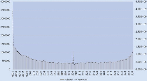
There are also some reasons for choosing the Chinese market. Firstly, there is strong evidence that closing price manipulation is serious in China (Allen et al. 2006, Ouyang and Cao 2020). It is worthwhile to test whether a closing call can alleviate manipulation or not. Secondly, although there already exist studies of this issue in Taiwan (Huang and Tsai 2008) or Hong Kong (Tong and Tse 2002), it would still be interesting to investigate this issue in the emerging markets of mainland China considering its inadequate regulation (Kong et al. 2020). Thirdly, we can see clear U-shaped trading patterns in the Shanghai Stock Exchange in Figure 1, consistent with previous studies (Wood et al. 1985, Heston et al. 2010). Would a call auction change this? This is an issue worth empirical testing.

Figure 1. The distribution of intraday trading before August 20, 2018. Notes: This figure shows the volume and amount traded every minute in Shanghai Stock Exchange before August 20, 2018. We could see clear U-shaped trading patterns in this figure.

Our empirical results show that volume in the last three minutes is significantly reduced. Volume in the minutes of continuous trading preceding the closing call increases dramatically, which indicates a shift of trading volume from the closing call to the preceding continuous trading. This is consistent with previous studies about liquidity demand (Foucault et al. 2005, Roşu 2009), order book opaqueness risks (Huang and Tsai 2008) and manipulation (Hillion and Suominen 2004, Chang et al. 2008). We also find a significant increase of volatility in the minutes of continuous trading preceding the closing call and a significant decrease of price deviation in the last three minutes’ closing call, which further supports that liquidity traders shift their orders to before the closing call (Chang et al. 2020). Because there are less liquidity noise and order imbalances, market efficiency is significantly improved (Kandel et al. 2012).

The remainder of the paper is organized as follows. Section 2 provides a brief review of related literature. Section 3 introduces our sample, data and methodology. Section 4 provides our empirical results and analysis. Section 5 concludes the paper.

2. Literature review

2.1. Volume & amount

There are lots of studies comparing the trading volume or amount under call auction and continuous trading. However, explanations and empirical findings are different. Those studies could be categorized into three groups, as follows:

The first group of studies would be represented by the information asymmetry models (Kyle 1985, Admati and Pfleiderer 1988, Kaniel and Liu 2006). Traders are divided into informed traders and uninformed traders in those studies. The underlying logic is that uninformed traders prefer to assemble to minimize their price impact, which results in the appearance of spikes of trading volume near closing. This is empirically consistent with U-shaped intraday patterns (Heston et al. 2010). Those studies indicate a shift in volume from the end of the continuous trading phase to the call auction (Kandel et al. 2012) because allowing for more rounds of trade would increase the expected profits of the informed, thereby hurting the uninformed traders (Kalay et al. 2002). Since all traders are given access to the same price simultaneously, call auction reduces information asymmetry costs and increases the trading volume (Madhavan 1992). It is supported by various empirical findings in different markets (Comerton-Forde et al. 2007, Kandel et al. 2012, Twu and Wang 2018).

Instead of a volume shift from continuous trading to call auction, there is also a group of findings that support a volume shift from call auction to continuous trading. It is argued that order book is fully opaque for the closing call period. Investors may close their position earlier than the closing period to avoid additional risk (Huang and Tsai 2008). Empirical studies in emerging markets like India find no evidence for volumes attracted by call auctions (Agarwalla et al. 2015). Some empirical studies in developed markets also show that stocks transferred from continuous trading to call auction would experience volume declines (Muscarella and Piwowar 2001). Although call auction can alleviate information asymmetry, it could also bring high information costs because of order book opaqueness (Ibikunle 2015). So investors may have a preference for closing their position under continuous trading (Lauterbach and Ungar 1997). Allowing for more trading rounds enables a better reaction to new information and improved risk-sharing (Brennan and Cao 1996). Lower frequency of trading will result in a smaller trading volume (Amihud et al. 1997, Kalay et al. 2002).

Another critical group of findings would be related to closing price manipulation. Closing price manipulation commonly involves aggressively buying or selling stocks at the end of a trading day to push the closing price to an artificial level. The manipulator seeks only to create a short-term liquidity imbalance, in many instances, just a matter of minutes (Comerton-Forde and Putniņš 2011). Many studies found that manipulation is serious near the closing, related to higher volume (Felixson and Pelli 1999, Comerton-Forde and Rydge 2006, Comerton-Forde et al. 2007, Comerton-Forde and Putniņš 2011). Carhart et al. (2002) find that market price manipulation in US equities markets is localized in the last half hour before the close. They attribute this phenomenon to manipulation by fund managers. Similarly, Hillion and Suominen (2004) find on the Paris Bourse that significant rises in volume occur mainly in the last minute of trading, and they attribute this to manipulation. However, the introduction of a call market at the end of the trading day reduces manipulation (Hillion and Suominen 2004, Chang et al. 2008) and would result in smaller trading volume. Many studies have proposed call auction sessions at the opening or closing of continuous auction sessions to ensure more efficient, manipulation-free prices (Muscarella and Piwowar 2001, Pagano and Schwartz 2003, Kadioglu et al. 2015). Manipulation is vital to our study in that many studies provide strong evidence for manipulation in the Chinese market (Allen et al. 2006, Ouyang and Cao 2020).

To sum up, the introduction of call auction could influence trading volume near the closing in several ways. Firstly, call auction would satisfy the liquidity need of uninformed traders in that it cuts the expected profits of the informed traders. So call auction would attract trading volume from the continuous auction. Secondly, because order book is fully opaque for the call period, investors may close their position earlier than the closing period to avoid additional risk. So we could see a shift of trading volume from call auction to preceding continuous trading. Thirdly, the introduction of call auction would reduce manipulations, which is related to high volume. So we could see a reduction of trading volume after the introduction of call auction.

Thus, it appears that determining which way dominates (if there is a clear dominance) or whether trading would increase or decrease under call auction is an empirical issue (Kalay et al. 2002).

We find a significant reduction in trading volume in the last 3 min in the Chinese market after introducing call auction. This is consistent with the order book opaqueness and manipulation findings. Investors may close their position earlier than the closing call auction to avoid additional price risks due to order book opaqueness. We also find a significant increase in trading volume in continuous trading before the closing call, which further supports the shift of trading volume from call auction to continuous trading. Our findings do not support those findings arguing that call auction would attract uninformed traders and increase trading volume, perhaps because those findings are mostly carried out in a dealer market rather than an order-driven market like China. In an order-driven market, the opaqueness of order book under call auction compared to continuous trading is more pronounced.

2.2. Price fluctuation

A variety of studies compare price fluctuation or price deviation under call auction and continuous trading. Price fluctuation is important because random price fluctuations and short-term volatility lead to illiquidity, inefficiency, and the investors’ discouragement from participating in financial markets (Stoll 2000). However, past studies do not come up with consistent conclusions. Those studies could be categorized into three groups, as follows:

The first group of studies would be represented by Amihud and Mendelson (1987). They find that open-to-open return volatility is higher than close-to-close volatility. They argue that this difference in volatility is due to the call auction at the open and the continuous trading at the close. The one-shot auction price at the open tends to deviate from the equilibrium price. In contrast, the price at the market close tends to be closer to the equilibrium price because the information is incorporated in the market through continuous trading. In that case, the open-to-open return distribution has a higher dispersion than the close-to-close return distribution. Many empirical studies provide evidence for this (Foster and Viswanathan 1990, Bogousslavsky and Muravyev 2020). However, it is argued that the higher open-to-open return volatility could well be due to the large amount of ‘unprocessed’ information that accumulates overnight before the market’s open, rather than to the call auction opening (Holden and Subrahmanyam 1992, Tong and Tse 2002). Studies in emerging markets like Hong Kong (Tong and Tse 2002) do not find such evidence. The conclusion that call auction would increase volatility involves endogeneity concerns and may not be robust.

Another group of studies would be represented by Admati and Pfleiderer (1991) using information asymmetry. They argue that there should be less of a price impact per unit of the trade when investors move their trades to an environment that gathers more liquidity. They also point out that volatility is more massive in a high-volume period than a low-volume period because the market maker faces less information asymmetry. Intuitively, a high volume is more likely to reflect high order imbalances (Daigler and Marilyn 1999, Bogousslavsky and Muravyev 2020). Under information asymmetry models, the call auction would attract trading volume from preceding continuous trading (Kyle 1985, Admati and Pfleiderer 1988, Kaniel and Liu 2006). Then we could see a reduction of volatility in minutes of continuous trading preceding the closing call. A contradictory explanation put forward by Kaniel and Liu (2006) relates this issue with information asymmetry too. But they argue that informed traders prefer continuous trading because their orders can be executed with a high degree of certainty at the market quotes (Lauterbach 2001). Knowing that they would not be allowed to trade continuously in the closing call, they would become more impatient and make more market orders and fewer limit orders in continuous trading preceding the closing call (Kandel et al. 2012). According to Kaniel and Liu (2006), an increase in the proportion of market orders submitted by informed traders implies an increase in volatility. This suggests that we could see an increase in volatility continuous trading minutes preceding the closing call.

Another group of studies would be represented by Foucault et al. (2005); Roşu (2009). They ignore informed traders but attach great importance to liquidity traders eager to close their unwanted inventory at the closing price (Chang et al. 2020). The underlying logic of this liquidity-based model is that those patient traders who play the role of liquidity suppliers tend to submit limit orders. In contrast, impatient traders who play the role of liquidity demanders usually submit market orders. Many investors, mutual funds, for example, have strong incentives to demand liquidity near the closing because both passively and actively managed mutual funds are subject to unexpected inflows and outflows of capital daily (Kandel et al. 2012). Those liquidity demanders would face a risk that their liquidity demand would not be satisfied in the closing call or carry their unwanted inventories overnight. They would like to close out their position in continuous trading and submit more market orders, thus increasing the volatility in continuous trading minutes preceding the closing call (Chang et al. 2020). Accentuated volatility of continuous trading before the closing call mainly indicates traders’ eagerness when trying to complete their trades before overnight (Inci and Ozenbas 2017). Empirical evidence from Taiwan Futures Exchange finds an increase in the volatility in minutes of continuous trading preceding the closing call after introducing call auction, due to diminishing investor patience (Chang et al. 2020). The empirical results in Taiwan Stock Exchange also show that the closing call has effectively reduced closing price deviation at the closing call by reducing liquidity noise in the last few minutes (Huang and Tsai 2008). The empirical results in Singapore also support this (Chang et al. 2008). Barclay et al. (2008) also show that call auctions are more likely to absorb extreme liquidity shocks without volatility. Those studies are consistent with the liquidity-based model in that they suggest a shift of liquidity traders from closing call to minutes of continuous trading preceding the closing call, thus decreasing the closing price deviation of call auction and increasing the price volatility in minutes of continuous trading preceding the call auction.

To sum up, three ways call auction could affect price fluctuation. Firstly, call auction would attract those uninformed traders because informed traders’ expected profits would be lower under call auction (Kalay et al. 2002). So there would be lower volume and lower volatility in minutes of continuous trading preceding the closing call. Secondly, those informed traders would be willing to trade under continuous trading and become impatient to trade in the closing call. They would submit market orders rather than limit orders in minutes of continuous trading preceding the closing call, thus increasing the volatility. Thirdly, those liquidity traders who are eager to close out their unwanted inventories would want to trade under continuous trading to mitigate their risks of failing to make a deal under call auction, thus increasing the volatility of preceding continuous trading.

Our findings are consistent with the second and third ways. We find significantly higher volatility in minutes of continuous trading preceding the closing call and a significantly lower closing call price deviation. This could be explained by the liquidity model (Roşu 2009) and is consistent with previous studies in Taiwan (Huang and Tsai 2008, Hennessy et al. 2020). Because more liquidity traders shift from the last three minutes of closing call to minutes of continuous trading preceding the closing call, the volatility of continuous trading preceding the closing call is higher now. Less liquidity noise is included in the closing call, and there would be less deviation of the closing price.

2.3. Market efficiency

The first group of studies would also be represented by the information asymmetry models proposed by Admati and Pfleiderer (1988). As we have already analyzed before, call auction would be more beneficial to uninformed investors because it reduces the expected profits of informed investors (Kalay et al. 2002). Because less-informed investors would participate in the closing call auction, the closing price’s information contents would be lower. It is also argued that the high volume attracted to the closing call can be noise caused by the uninformed traders. For example, many mutual funds may want to buy or sell at closing prices to create a benchmark. Such a benchmark targeting volume would not provide any additional useful information to closing price (Frei and Mitra 2020). Empirical studies also provide evidence for this (Asparouhova et al. 2013, 2010, Bogousslavsky and Muravyev 2020). Some studies argue that although the adverse selection costs are significantly lower under the call auction. However, there is no significant reduction in average price efficiency (Schnitzlein 1996).

The second group of studies would be represented by the liquidity-based model (Foucault et al. 2005, Roşu 2009). It is argued that those liquidity traders would prefer trading under continuous trading for fear of carrying their unwanted inventories overnight. So they would close out their positions in minutes of continuous trading preceding the closing call. By reducing liquidity noise in the closing auction, the closing price is more efficient now (Kandel et al. 2012). Large quantities of empirical studies have provided evidence for this improvement in different markets such as Taiwan (Huang and Tsai 2008), Singapore (Comerton-Forde et al. 2007), India (Agarwalla et al. 2015), Borsa Istanbul (Kandel et al. 2012), Borsa Italiana (Kandel et al. 2012), NASDAQ (Barclay et al. 2008, Pagano et al. 2013), Euronext Paris (Pagano and Schwartz 2003), Australia (Comerton-Forde and Rydge 2006), London (Ellul et al. 2005, Chelley-Steeley 2009, 2008, Ibikunle 2015). Some empirical evidence also supports this view in other markets such as the futures markets (Cheng and Kang 2007, Hagströmer and Nordén 2014, Chang et al. 2020), precious metal market (Aspris et al. 2020) etc.

Another group of studies would be related to manipulation. It has already been discussed before that the manipulator seeks only to create a short-term liquidity imbalance, in many instances, just a matter of minutes (Comerton-Forde and Putniņš 2011). Barclay et al. (2008) study markets’ ability to absorb order imbalances. Such order imbalances can temporarily affect financial markets prices even if these imbalances reveal little or no information about fundamental values. Because these distortions reduce the efficiency of prices and adversely affect traders in both spot and derivative markets (Hagströmer and Nordén 2014), an essential aspect of financial market efficiency is the ability to absorb liquidity shocks and minimize temporary price changes. However, the introduction of a call market at the end of the trading day reduces manipulation (Hillion and Suominen 2004, Chang et al. 2008) and would result in more efficient closing prices.

To sum up, several aspects could decide the impact of call auction on market efficiency. Firstly, call auction would attract many uninformed traders (e.g. traders eager to create a benchmark at closing price), but those traders do not provide any information about fundamental values. So the introduction of call auction may hamper market efficiency. Secondly, call auction imposes a risk of not making a deal on those liquidity traders, thus shifting those liquidity noises to minutes of continuous trading preceding the closing call, which would result in an improvement of market efficiency. Thirdly, call auction makes it harder for manipulators to manipulate the closing price by imbalances, thus improving market efficiency.

We use three main methods in testing market efficiency that has been assessed in the previous literature (Pagano et al. 2013): (1) by assessing the cross-sectional synchronicity of price formation at market openings and closings (Pagano et al. 2013). (2) by contrasting the magnitude of daily open-to-open return and close-to-close return (Amihud and Mendelson 1987). (3) by examining price behaviors in minutes that precede the close (Kandel et al. 2012). All provide evidence that market efficiency has been improved by introducing the call auction, which supports the second and third ways.

Finally, we sum up our review in Table 1.

Table 1. Conclusions of literature review.

	Information asymmetry	Liquidity demand	Manipulation
Intuitional Explanation	Uninformed traders would prefer trading under call auction because the expected profits of informed traders would be lower, and they could construct a benchmark using the closing price. This would shift uninformed traders from preceding continuous trading to the closing call, thus lowering closing price efficiency.	Liquidity traders would bear the risk of not making a deal under the single closing call auction. So they would shift their volume from the closing call to preceding continuous auction. This reduces liquidity noise in closing price and increases volatility in minutes of continuous trading preceding the closing call.	Call auction makes it harder for manipulators to make use of order imbalances. It reduces those manipulations and stabilizes the market near closing, thus improving market efficiency.
Volume in the Closing Call	↑	↓	↓
Volume in Minutes of Continuous trading Preceding the Closing Call	↓	↑	Not Mentioned
Volatility in Minutes of Continuous trading Preceding the Closing Call	↓	↑	Not Mentioned
Closing Price deviation	↑	↓	↓
Price Synchronicity	↓	↑	↑
Open-to-Open to Close-to-Close Efficiency	↓	↑	↑
Representative Literature	Admati and Pfleiderer (1988)	Foucault et al. (2005), Roşu (2009)	Hillion and Suominen (2004)
Consistent with Our Findings?	No	Yes	Yes

Notes: In this table we sum up our literature review. ↑ represents increase and ↓ represents decrease.

3. Data, variables and methodology

3.1. Sample and data

Our sample is based on all A-share listed companies of the Shanghai Stock Exchange and Shenzhen Stock Exchange from January 1, 2017 to December 31, 2019. We calculate a daily index for each stock using high-frequency data of every minute. For example, when we test the last 3 min trading volume, we sum up the number of shares traded for a given stock in the last three minutes for each day.

Table 2. Definitions of control variables.

Variables	Meaning and calculation method
ma5	A 5-day moving average calculated using the average price over the past five days.
bbi	BBI technical indicators.
macd	MACD technical indicators.
sar	SAR technical indicators of parabolic inversion.
beta	The systemic risk coefficient of the stock calculated using CAPM model.
turnover	Turnover, volume divided by the total number of circulating shares.
dominant_buy_ratio	The proportion of active buying transaction amount to total transaction amount.
roa	Net profit divided by total assets.
eps	Net profit divided by the number of shares outstanding.
pe	Price per share divided by earnings per share.
lev	Total liabilities divided by total assets.
market_value	The number of shares in circulation multiplied by the market price of each share.
gross_profit_margin	Sales revenue minus sales cost, divided by sales revenue.
operating_profit_growth	The operating profit of the current period minus the operating profit of the previous period, and then divided by the operating profit of the previous period.
operating_revenue	Total operating revenue.

Note: In this table we define our control variables.

Here are several reasons why we choose this period. Firstly, all the stocks in the Shanghai Stock Exchange experienced a trading mechanism change in this period, but the stocks in the Shenzhen Stock Exchange had already experienced this in 2006. This gives us a chance to construct an experiment using the difference-in-difference model mentioned later. Secondly, because we use high-frequency data to test the effects of trading mechanism change empirically, three years from 2017 to 2019 would be a sample large enough to derive reliable conclusions. Thirdly, this sample contains the most recent years’ observations, and relevant data are accessible to have a consistent sample period for various tests. Finally, although they are not symmetric, they are three full fiscal years. We will also change the sample period to ensure the robustness of our findings. We will also construct a symmetric sample period around the introduction of the closing auction on August 20, 2018, in our robustness checks to ensure our conclusions’ reliability.

We deleted all the missing observations before the empirical tests. Our data are derived from the Wind database. We finally obtained 2,436,106 stock-day observations as our research sample.

3.2. Explanation of our models

To construct a difference-in-difference model in reference to Hennessy et al. (2020), we divide the full sample into two parts, the treat group and the control group. The first subsample contains stocks traded in the Shanghai Stock Exchange, and the second subsample contains stocks traded in the Shenzhen Stock Exchange. Shanghai is the treat group that has experienced a change of trading mechanism, but Shenzhen is the control group that has not. We define a variable denoted $treated$ to distinguish between stocks in the Shanghai Stock Exchange and stocks in the Shenzhen Stock Exchange. It would be 1 if a stock is in the treat group (Shanghai) and be 0 if the stock is in the control group (Shenzhen).

We also need a variable to distinguish whether the policy has been carried out or not in a standard difference-in-difference model. In reference to a standard difference-in-difference model of Hennessy et al. (2020), we define a variable denoted $period$ to distinguish the period before the change of trading mechanism and after the change of trading mechanism. Specifically, trading days before August 20, 2018, would be 0 and trading days after August 20, 2018, would be 1. The difference-in-difference variable $treated\mathrm{\_}period$ is defined as $treated$ multiply $period$. It can be confusing why we define variables this way. We define those variables in reference to the difference-in-difference model widely used in recent research (Butler and Cornaggia 2011, Heimer and Simsek 2019, Hennessy et al. 2020) to evaluate the effects of policies. Let us explain the logic as follows:

As is shown in Figure 2, we define $period$ because we have to consider individual differences. Specifically, if we compare $Shangha{i}_1$ and $Shenzhe{n}_1$ to find the effects of the introduction of call auction, we ignore that they have some characteristics different. For example, the Shanghai Stock Exchange has less listed companies than the Shenzhen Stock Exchange. However, if we just compare $Shangha{i}_1$ with $Shangha{i}_0$, we ignore the fact that there are some factors other than the trading mechanism influencing the Chinese stock market. For example, macroeconomic uncertainties during this period may affect the trading behaviors of Chinese stocks. Then we could not conclude that it is the introduction of call auction that has changed the trading behaviors. This is why we need the variable $treated$, which can help us find a comparative group, the Shenzhen Stock Exchange, to mitigate unobservable macroeconomic changes. So the difference-in-difference variable $treated\mathrm{\_}period$ would be an unbiased estimation of the effects of the introduction of the call auction, which is widely used in the recent literature of causality inference (Heimer and Simsek 2019, Chan et al. 2020, Hennessy et al. 2020).

Figure 2. An illustration of DID model. Notes: In this figure we illustrate the main idea of difference-in-difference model. 0 means period before August 20, 2018 and 1 means period after it.

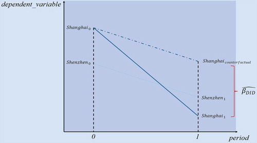
A key assumption for the unbiased estimation of the difference-in-difference model is that the Shanghai Stock Exchange should have a parallel trend during this period, so we carry out parallel trend tests later on.

3.3. Tests for volume & amount

Firstly, we will test whether the introduction of call auction significantly affects the trading volume and trading amount of the last three minutes. For every trading day of each company, we calculate the total number of shares that are traded for this company in the last three minutes before closing (i.e. from 14:57 to 15:00). We define this variable as $total\mathrm{\_}volume$. We define $total\mathrm{\_}amount$ as the total amount of transactions in the last three minutes (i.e. from 14:57 to 15:00). It is calculated by the total number of shares traded in the last three minutes multiply the unique price set by call auction. Under continuous trading, it is calculated by the sum of each minute’s trading amount.

In reference to Heimer and Simsek (2019), we construct the difference-in-difference model as follows: (1) $\begin{array}{rl}total\mathrm{\_}volum{e}_{i,t}& ={\text{β}}_0+{\text{β}}_{1}treated\mathrm{\_}perio{d}_{i,t}+{\text{β}}_{2}perio{d}_{i,t}\\ & +{\text{β}}_{3}treate{d}_{i,t}+{\text{β}}_{4}Control{s}_{i,t}+{\epsilon }_{i,t}\end{array}$(1) (2) $\begin{array}{rl}total\mathrm{\_}amoun{t}_{i,t}& ={\text{β}}_0+{\text{β}}_{1}treated\mathrm{\_}perio{d}_{i,t}+{\text{β}}_{2}perio{d}_{i,t}\\ & +{\text{β}}_{3}treate{d}_{i,t}+{\text{β}}_{4}Control{s}_{i,t}+{\epsilon }_{i,t}\end{array}$(2)

In those formulas, $i$ represents company and $t$ represents trading day. $Controls$ represents the controlled variable (Table 2).

In this paper, various technical indicators and financial indicators that may affect the transaction behaviors are controlled. We take into account technical indicators because many previous studies suggest a strong relationship between them and trading volume (Lee and Swaminathan 2000, Brown et al. 2009). We take into account financial indicators because companies in different financial positions can be traded very differently (Weigand 1996, Brown et al. 2009). For example, those large companies are more like to be frequently traded by institutional investors in contrast to those small companies. The trading behaviors could be influenced significantly by indicators in quarterly financial reports. We have to control those variables to identify the trading mechanism’s effects. We use these indicators that could be found in quarterly reports and then transform them to a daily basis. For example, March 22th and March 23th would have an identical value for the financial leverage variable, derived from the first quarter’s financial reports. This transformation method is widely used in quantitative trading strategy research or practical quantitative portfolio management because most quantitative transactions are conducted daily. Managers would use financial factors accompanied by technical indicators to discern good companies. It is just similar to controlling for firm-specific effects in corporate financial studies. The specific definitions for control variables are as follows:

Some unobservable factors of specific firms or specific trading days may still exist, resulting in endogeneity problems. We further use the two-way fixed effects model to control the fixed effect at the firm level and trading day level with reference to Heimer and Simsek (2019) to alleviate the problem of potential missing variables. The specific model is as follows: (3) $\begin{array}{rl}total\mathrm{\_}volum{e}_{i,t}& ={\text{β}}_0+{\text{β}}_{1}treated\mathrm{\_}perio{d}_{i,t}+{\text{β}}_{2}Control{s}_{i,t}\\ & +u_i+{\lambda }_t+{\epsilon }_{i,t}\end{array}$(3) (4) $\begin{array}{rl}total\mathrm{\_}amoun{t}_{i,t}& ={\text{β}}_0+{\text{β}}_{1}treated\mathrm{\_}perio{d}_{i,t}+{\text{β}}_{2}Control{s}_{i,t}\\ & +u_i+{\lambda }_t+{\epsilon }_{i,t}\end{array}$(4)

Among them, $u_i$ is the fixed effect of the company, and ${\lambda }_t$ is the fixed effect of the trading day. Note that we have removed the variables $perio{d}_{i,t}$ and $treate{d}_{i,t}$ now, because we have controlled every specific company and every trading day. If they are added to equations, there would be complete collinearity. We deal with it with reference to Heimer and Simsek (2019).

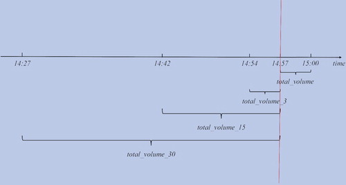
Finally, we should also test whether call auction has a significant impact on volume and amount before the closing call to justify a shift of trading volume from call auction to preceding continuous trading as investors want to avoid additional risks related to the opaqueness of the order book (Huang and Tsai 2008). We calculate the total volume and amount in 3, 15 and 30 min before call auction and define them as $total\mathrm{\_}volume\mathrm{\_}n$ and $total\mathrm{\_}amount\mathrm{\_}n$ ($n=1,15,30$). It is illustrated in Figure 3, specifically. Then we construct the difference-in-difference models the same as before to test the call auction’s effects on trading behaviors in continuous trading preceding the closing call auction. All the independent variables have identical definitions as before. (5) $\begin{array}{rl}total\mathrm{\_}volume\mathrm{\_}{n}_{i,t}& ={\text{β}}_0+{\text{β}}_{1}treated\mathrm{\_}perio{d}_{i,t}\\ & +{\text{β}}_{2}perio{d}_{i,t}+{\text{β}}_{3}treate{d}_{i,t}\\ & +{\text{β}}_{4}Control{s}_{i,t}+{\epsilon }_{i,t}\end{array}$(5) (6) $\begin{array}{rl}total\mathrm{\_}amount\mathrm{\_}{n}_{i,t}& ={\text{β}}_0+{\text{β}}_{1}treated\mathrm{\_}perio{d}_{i,t}\\ & +{\text{β}}_{2}perio{d}_{i,t}+{\text{β}}_{3}treate{d}_{i,t}\\ & +{\text{β}}_{4}Control{s}_{i,t}+{\epsilon }_{i,t}\end{array}$(6)

Figure 3. The method of calculating volume & amount shift. Notes: In this figure we explain how we calculate volume in continuous trading preceding the closing call.

We also construct symmetric samples of different window period to ensure the robustness of conclusions.

3.4. Tests for price fluctuation

From Figure 1, we could find that there is a clear upward trend of trading near the closing. It is found by past research that high volume is significantly related to price fluctuation (Daigler and Marilyn 1999). Would the call auction reduce the price fluctuation near the closing, thus stabilizing the closing price? We will test it now.

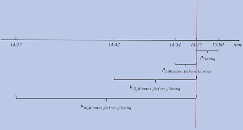
Because under call auction, a single unique price is set in the last three minutes. It would be meaningless to calculate volatility under call auction and compare it to continuous trading. It is also meaningless to calculate the difference between high and low to describe price fluctuation because a unique price is set under call auction, and such variables would be zero.

Instead, we could calculate the difference between the closing price determined in the last three minutes and the volume-weighted average price before the closing three minutes. This is intuitional in that it can measure the extent to which closing price deviates from the average price before closing. Specifically, we calculate both absolute price difference $abs$ and normalized absolute price difference $nabs$ in reference to Inci and Ozenbas (2017).

As is shown in Figure 4, we will use the volume-weighted price under continuous trading and the unique price set under call auction in the last three minutes to derive a price called $P_{closing}$. Then we will calculate the volume-weighted price before the closing three minutes. We use several time intervals (i.e. 3, 15 and 30 min). We choose 3 min because it exactly equals the closing time interval so that they are comparable. We choose 15 min and 30 min because they can reflect a much more stable price before closing and can be used to measure the extent to which closing price deviates from this relatively stable price. Then we get $P_{n\mathrm{\_}Minutes\mathrm{\_}Before\mathrm{\_}Closing}$ ($n=3,15,30$), and we can define the $ab{s}_n$ and $nab{s}_n$ as follows: (7) $\begin{array}{rl}ab{s}_n& =|P_{closing}-P_{n\mathrm{\_}Minutes\mathrm{\_}Before\mathrm{\_}Closing}|\end{array}$(7) (8) $\begin{array}{rl}nab{s}_n& =\left|\frac{P_{closing}-P_{n\mathrm{\_}Minutes\mathrm{\_}Before\mathrm{\_}Closing}}{P_{n\mathrm{\_}Minutes\mathrm{\_}Before\mathrm{\_}Closing}}\right|\end{array}$(8)

Figure 4. The method of calculating price fluctuation. Notes: In this figure we explain how we calculate price deviation of last three minutes to preceding minutes.

Similar to above, we constructed difference-in-difference models and two-way fixed effects models to conduct our empirical tests. The definitions of $treated\mathrm{\_}period$, $period$ and $treated$ are entirely identical to above, so do the definitions of control variables. The regression equations are listed as follows: (9) $\begin{array}{rl}ab{s}_{i,t}& ={\text{β}}_0+{\text{β}}_{1}treated\mathrm{\_}perio{d}_{i,t}+{\text{β}}_{2}perio{d}_{i,t}\\ & +{\text{β}}_{3}treate{d}_{i,t}+{\text{β}}_{4}Control{s}_{i,t}+{\epsilon }_{i,t}\end{array}$(9) (10) $\begin{array}{rl}ab{s}_{i,t}& ={\text{β}}_0+{\text{β}}_{1}treated\mathrm{\_}perio{d}_{i,t}+{\text{β}}_{2}Control{s}_{i,t}\\ & +u_i+{\lambda }_t+{\epsilon }_{i,t}\end{array}$(10) (11) $\begin{array}{rl}nab{s}_{i,t}& ={\text{β}}_0+{\text{β}}_{1}treated\mathrm{\_}perio{d}_{i,t}+{\text{β}}_{2}perio{d}_{i,t}\\ & +{\text{β}}_{3}treate{d}_{i,t}+{\text{β}}_{4}Control{s}_{i,t}+{\epsilon }_{i,t}\end{array}$(11) (12) $\begin{array}{rl}nab{s}_{i,t}& ={\text{β}}_0+{\text{β}}_{1}treated\mathrm{\_}perio{d}_{i,t}+{\text{β}}_{2}Control{s}_{i,t}\\ & +u_i+{\lambda }_t+{\epsilon }_{i,t}\end{array}$(12)

We also carried out parallel trend tests and placebo tests to ensure the robustness of our conclusion.

As is mentioned before, we also need to compare the volatility in minutes of continuous trading preceding the closing call to justify that our conclusions are consistent with models of Foucault et al. (2005), Roşu (2009) and Kaniel and Liu (2006). We calculate the volume-weighted volatility under continuous trading preceding the closing call in reference to Chang et al. (2020). Specifically, we calculate the volatility of 14:54 to 14:57, 14:42 to 14:57 and 14:27 to 14:57 (3, 15 and 30 min respectively, consistent with above), and denote them as $volatility\mathrm{\_}n$ ($n=3,15,30$). Similar to above, we constructed difference-in-difference models, two-way fixed effects models to conduct our empirical tests. The definitions of $treated\mathrm{\_}period$, $period$ and $treated$ are completely identical to above, so do the definitions of control variable. The regression equations are listed as follows: (13) $\begin{array}{rl}volatility\mathrm{\_}{n}_{i,t}& ={\text{β}}_0+{\text{β}}_{1}treated\mathrm{\_}perio{d}_{i,t}+{\text{β}}_{2}perio{d}_{i,t}\\ & +{\text{β}}_{3}treate{d}_{i,t}+{\text{β}}_{4}Control{s}_{i,t}+{\epsilon }_{i,t}\end{array}$(13) (14) $\begin{array}{rl}volatility\mathrm{\_}{n}_{i,t}& ={\text{β}}_0+{\text{β}}_{1}treated\mathrm{\_}perio{d}_{i,t}+{\text{β}}_{2}Control{s}_{i,t}\\ & +u_i+{\lambda }_t+{\epsilon }_{i,t}\end{array}$(14)

We also construct subsamples of different symmetric windows to ensure the robustness of our conclusions.

3.5. Tests for market efficiency

We construct a three-stages regression model in reference to (Pagano and Schwartz 2003, Chelley-Steeley 2009) to test the call auction’s impact on market efficiency.

Firstly, we choose the sample period from January 1, 2017 to December 31, 2019, to be consistent with the tests above. We will also construct a symmetric sample of 250 days and 120 days in reference to Pagano and Schwartz (2003) as robustness checks. We will not include 60 days, 20 days and 10 days sample in that they are too short to conduct a three-stages regression. We also define $treated$,$period$, and $treated\mathrm{\_}period$ the same as before to carry out the difference-in-difference model. We calculate their daily logarithmic returns together with market returns to construct the first-stage regression: (15) $R_{j,L,period,t}={\alpha }_{j,L}+{\text{β}}_{j,L,period}{R}_{m,L,period,t}+{\xi }_{j,L,period,t}$(15)

In the above equation, $L$ represents the time interval to calculate logarithmic returns. For example, one day return, two days’ return, etc. We choose 1 trading day to 20 trading days in reference to Pagano and Schwartz (2003). $R_{j,L,period,t}$ represents the return of the company $j$ at the time $t$. $R_{m,L,period,t}$ represents the market return at time $t$. We estimate the $\widehat{{\text{β}}_{j,L,period}}$ for each stock under different $L$ and $period$.

Then we collect all the $\widehat{{\text{β}}_{j,L,period}}$ derived from first-stage regression as dependent variables in second-stage regression: (16) $\widehat{{\text{β}}_{j,L,period}}=a_{j,period}+b_{j,period}\ln (1+L^{-1})+{\gamma }_{j,L,period}$(16)

We can estimate $\widehat{a_{j,period}}$ and $\widehat{b_{j,period}}$ for each company $j$ during each $period$. If $\widehat{b_{j,period}}$ is significantly positive, it indicates that $\widehat{{\text{β}}_{j,L,period}}$ is negatively associated with $L$, thus an overreaction to information. If $\widehat{b_{j,period}}$ is significantly negative, it indicates $\widehat{{\text{β}}_{j,L,period}}$ is positively associated with $L$, thus an underreaction to information. The closer $\widehat{b_{j,period}}$ is to zero, the more efficient the market is. Finally, we construct a difference-in-difference model consistent with the above to test whether the introduction of call auction influences the market efficiency. (17) $\begin{array}{rl}|\widehat{b_{j,period}}|& ={\text{β}}_0+{\text{β}}_{1}treated\mathrm{\_}perio{d}_{j,period}+{\text{β}}_{2}perio{d}_{j,period}\\ & +{\text{β}}_{3}treate{d}_{j,period}+{\epsilon }_{j,period}\end{array}$(17) (18) $\begin{array}{rl}\widehat{b_{j,period}}& ={\text{β}}_0+{\text{β}}_{1}treated\mathrm{\_}perio{d}_{j,period}+{\text{β}}_{2}perio{d}_{j,period}\\ & +{\text{β}}_{3}treate{d}_{j,period}+{\epsilon }_{j,period},\\ & for\widehat{b_{j,period}}>0\end{array}$(18) (19) $\begin{array}{rl}\widehat{b_{j,period}}& ={\text{β}}_0+{\text{β}}_{1}treated\mathrm{\_}perio{d}_{j,period}+{\text{β}}_{2}perio{d}_{j,period}\\ & +{\text{β}}_{3}treate{d}_{j,period}+{\epsilon }_{j,period},\\ & for\widehat{b_{j,period}}<0\end{array}$(19)

If the introduction of call auction improve the market efficiency, it should have positive effects on those $\widehat{b_{j,period}}<0$, and negative effects on those $\widehat{b_{j,period}}>0$ to bring them more close to zero, thus lowering the absolute value $|\widehat{b_{j,period}}|$.

To ensure our tests’ robustness, we construct an alternative dependent variable proposed by Stoll (2000) as a robustness check. Specifically, Stoll (2000), among others (Chang et al. 2008), suggests that the ratio of open-to-open returns to close-to-close returns is another way to see if a change at the closing of a market has affected the quality of trading within a market. Ideally, this ratio should be close to 1.0 and thus any detrimental market structure change would be expected to result in this ratio deviating further away from 1.0. We calculate the daily close-to-close returns and open-to-open returns of A-share listed companies in the Shanghai Stock Exchange and the Shenzhen Stock Exchange from January 1, 2017, to December 31, 2019, which is consistent with the above tests. We also construct several symmetric subsamples of 250 days, 60 days and 20 days consistent with the above tests to ensure our conclusions’ robustness. The dependent variable is defined as follows: (20) $abs\mathrm{\_}VR\mathrm{\_}{1}_{i,t}=\left|\frac{open-to-openretur{n}_{i,t}}{close-to-closeretur{n}_{i,t}}-1\right|$(20)

It can measure the deviation of open-to-open return to close-to-close return ratio to 1.0. The smaller this indicator is, the more efficient the market is. We construct the difference-in-difference model and two-way fixed effects model the same as before, where independent variables are defined identically to previous tests. (21) $\begin{array}{rl}abs\mathrm{\_}VR\mathrm{\_}{1}_{i,t}& ={\text{β}}_0+{\text{β}}_{1}treated\mathrm{\_}perio{d}_{i,t}+{\text{β}}_{2}perio{d}_{i,t}\\ & +{\text{β}}_{3}treate{d}_{i,t}+{\text{β}}_{4}Control{s}_{i,t}+{\epsilon }_{i,t}\end{array}$(21) (22) $\begin{array}{rl}abs\mathrm{\_}VR\mathrm{\_}{1}_{i,t}& ={\text{β}}_0+{\text{β}}_{1}treated\mathrm{\_}perio{d}_{i,t}+{\text{β}}_{2}Control{s}_{i,t}\\ & +u_i+{\lambda }_t+{\epsilon }_{i,t}\end{array}$(22)

4. Empirical results and analysis

4.1. Descriptive statistics

We sum up the descriptive statistics of this paper in Table 3. As is shown in the table, the values of all variables are within a reasonable range. The average of $total\mathrm{\_}amount$ is about 2,212,000 yuan, indicating that the transaction amount in the last three minutes near closing is huge in the Chinese market. The average of $total\mathrm{\_}volume$ is 198,200 shares (one round lot equals 100 shares in China, and we call it ‘a hand’ in Chinese), which further supports for the view that the trading volume near the closing is huge in the Chinese market. The average of $ab{s}_n$ is increasing with the time interval $n$, which indicates that a longer time interval would result in larger price fluctuation, which is consistent with intuition. For other technical indicators and corporate financial indicators, their values are within reasonable ranges, so the following regression analysis is carried out.

Table 3. Descriptive statistics.

	(1)	(2)	(3)	(4)	(5)
Variables	N	Mean	SD	Min	Max
total_volume	2.436e+06	1,982	5,668	0	884,114
total_amount	2.436e+06	2.212e+06	6.225e+06	0	1.342e+09
total_amount_3	2.436e+06	2.891e+06	6.609e+06	0	9.815e+08
total_amount_15	2.436e+06	1.105e+07	2.505e+07	0	3.734e+09
total_amount_30	2.436e+06	1.877e+07	4.233e+07	0	5.362e+09
total_volume_3	2.436e+06	2,647	6,646	0	1.297e+06
total_volume_15	2.436e+06	10,066	24,588	0	4.508e+06
total_volume_30	2.436e+06	17,066	41,980	0	8.320e+06
abs_3	2.436e+06	0.0168	0.0387	0	4.160
abs_15	2.436e+06	0.0360	0.0788	0	7.176
abs_30	2.436e+06	0.0500	0.109	0	8.923
nabs_3	2.436e+06	0.00109	0.00147	0	0.109
nabs_15	2.436e+06	0.00223	0.00277	0	0.179
nabs_30	2.436e+06	0.00303	0.00370	0	0.188
volatility_3	2.436e+06	0.0160	0.0318	0	4.596
volatility_15	2.436e+06	0.0312	0.0549	0	4.354
volatility_30	2.436e+06	0.0416	0.0738	0	5.774
VR	2.353e+06	−0.0328	8.453	−1,903	1,373
VR_1	2.353e+06	−1.033	8.453	−1,904	1,372
abs_VR_1	2.353e+06	3.010	7.966	0	1,904
treated_period	2.436e+06	0.198	0.399	0	1
treated	2.436e+06	0.405	0.491	0	1
period	2.436e+06	0.488	0.500	0	1
ma5	2.436e+06	13.97	10.12	0	51.23
bbi	2.436e+06	14.04	10.14	0	50.67
macd	2.436e+06	0.00803	0.234	−1.452	1.135
sar	2.436e+06	14.10	10.22	0	51.81
beta	2.436e+06	0.968	0.725	−4.722	8.022
turnover	2.436e+06	1.803	1.706	0	14.55
dominant_buy_ratio	2.436e+06	0.459	0.0973	0	0.962
pe	2.436e+06	52.78	49.42	0	308.5
market_value	2.436e+06	589,485	499,439	9,554	2.185e+06
roa	2.436e+06	4.330	5.211	−11.75	18.26
eps	2.436e+06	0.215	0.275	−0.768	1.220
lev	2.436e+06	42.00	21.64	0	136.1
gross_profit_margin	2.436e+06	9.233	11.87	−25.82	38.78
operating_profit_growth	2.436e+06	23.82	90.34	−189.5	215.6
operating_revenue	2.436e+06	3.163e+09	2.927e+09	−2.649e+09	9.195e+09

Notes: “N” represents number of observations in our regression sample, “mean” represents the mean value of this variable in our sample, “sd” represents the standard deviation of this variable in our sample, “min” and “max” represent minimum and maximum value of this variable in our sample.

4.2. Empirical test results of volume & amount

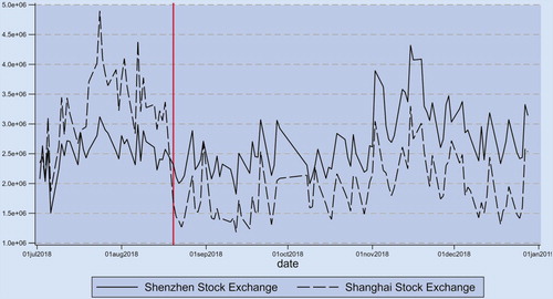
Firstly, we illustrate the daily volume in the last three minutes near closing in Figure 5. The left part of the red line represents volume under continuous trading, and the right part of the red line represents volume under call auction. It can be seen from the figure that the volume and amount of the Shanghai Stock Exchange are significantly higher than that of the Shenzhen Stock Exchange under continuous trading. However, the volume and amount of the Shanghai Stock Exchange are significantly lower than that of the Shenzhen Stock Exchange under call auction. This reflects that call auction can reduce the trading volume and trading amount near the closing. Call auction may alleviate the excessive trading near the closing, which is described before in the Chinese market.

Figure 5. Time series of total volume in last three minutes of different exchanges. Notes: In this figure we compare the total volume of last three minutes in Shanghai Stock Exchange and Shenzhen Stock Exchange respectively. We could see a clear decrease of volume in Shanghai Stock Exchange after the introduction of call auction.

According to the difference-in-difference model described above, the Shanghai Stock Exchange is taken as the treat group, and the Shenzhen Stock Exchange is taken as the control group to explore the impact of call auction on volume and amount in last three minutes. The empirical test results are shown in Table 4.

Table 4. DID tests for volume and amount.

	(1)	(2)	(3)	(4)	(5)	(6)
Variables	total_volume	total_amount	total_volume	total_amount	total_volume	total_amount
treated_period	−1,895***	−1.883e+06***	−1,373***	−1.521e+06***	−1,364***	−1.515e+06***
	(14.67)	(16,097)	(13.51)	(14,816)	(13.49)	(14,795)
treated	2,013***	2.016e+06***	1,488***	1.630e+06***	1,414***	1.535e+06***
	(10.25)	(11,250)	(9.523)	(10,446)	(9.548)	(10,475)
period	341.7***	−211,227***	−34.47***	302,872***	−17.74*	296,517***
	(9.341)	(10,248)	(9.082)	(9,962)	(9.166)	(10,056)
ma5			−76.10***	71,320***	−79.83***	64,312***
			(3.851)	(4,224)	(3.843)	(4,216)
bbi			−2.485	38,111***	21.49***	56,685***
			(4.079)	(4,474)	(4.084)	(4,480)
macd			−227.1***	70,682***	−186.1***	114,845***
			(16.66)	(18,271)	(16.62)	(18,228)
sar			−44.20***	−87,179***	−46.36***	−84,584***
			(3.413)	(3,743)	(3.407)	(3,738)
beta			2.192	135,900***	4.473	139,231***
			(4.612)	(5,059)	(4.598)	(5,044)
turnover			990.7***	1.008e+06***	986.4***	1.006e+06***
			(2.182)	(2,393)	(2.181)	(2,392)
dominant_buy_ratio			1,440***	1.751e+06***	1,423***	1.738e+06***
			(34.49)	(37,829)	(34.39)	(37,724)
pe			2.466***	4,337***	2.200***	4,540***
			(0.0704)	(77.23)	(0.0766)	(84.05)
market_value			0.00375***	4.297***	0.00349***	3.965***
			(7.10e−06)	(0.00778)	(9.39e−06)	(0.0103)
roa					−99.87***	−98,235***
					(1.233)	(1,353)
eps					38.01**	429,713***
					(16.60)	(18,210)
lev					9.785***	11,914***
					(0.202)	(221.8)
gross_profit_margin					33.81***	30,930***
					(0.454)	(498.0)
operating_profit_growth					0.287***	567.6***
					(0.0429)	(47.08)
operating_revenue					2.89e−08***	3.17e−05***
					(1.82e−09)	(2.00e−06)
Constant	1,376***	1.871e+06***	−1,401***	−4.113e+06***	−1,851***	−4.647e+06***
	(6.517)	(7,149)	(18.72)	(20,530)	(20.50)	(22,488)
Observations	2,436,106	2,436,106	2,436,106	2,436,106	2,436,106	2,436,106
R-squared	0.017	0.019	0.172	0.174	0.177	0.179

Notes: Standard errors in parentheses ***p < 0.01, **p < 0.05, *p < 0.1, Observations represent number of observations in our regression sample.

From Table 4, we can see that the coefficients of the difference-in-difference variable $treated\mathrm{\_}period$ are all negative and significant at the 1% level. The introduction of call auction would result in trading volume in the last three minutes to decrease about 130,000 shares as our regressions indicate. It also reduces the trading amount near the closing for about 1,500,000 yuan in our regressions. This indicates that the introduction of call auction would significantly reduce the excessive trading near the closing from both perspectives of volume and amount.

As for control variables, the coefficients are consistent with prior research. For example, we find that trading volume is positively associated with large firms, which is significant at the 1% level. This is consistent with the previous findings (Brown et al. 2009, Weigand 1996). Another example would be the positive relationship between PE ratio and trading volume, which is also consistent with the previous study (Brown et al. 2009). We also find that the technical indicator of momentum (i.e. moving average) is negatively associated with the trading volume, which is consistent with previous studies (Brown et al. 2009, Lee and Swaminathan 2000) too.

It is mentioned before that several control variables could only be obtained from quarterly reports of companies, which could be a concern to influence the accuracy of our regression. So we also carry out regressions without those control variables in Table 4. It seems that those variables would not have a material impact on the coefficients of our regressions. We also have to consider about sample period concern, which would be discussed later as robustness checks.

In order to mitigate the unobservable factors of companies and trading days that could cause the endogeneity problem, we control company fixed effects and trading day fixed effects in reference to Heimer and Simsek (2019). The results are shown in Appendix 1. The regression results are almost the same as Table 4. We can see that the coefficients of $treated\mathrm{\_}period$ are still negative and significant at the 1% level. This further demonstrates that the introduction of call auction would significantly reduce the trading volume and amount even after controlling fixed effects of companies and trading days.

It has been illustrated that we choose the sample period of 2017–2019 according to the fiscal year, which is not symmetric around the introduction of the closing auction on August 20, 2018. We have to change the window length as well as construct a symmetric sample around August 20, 2018, to ensure the robustness of our findings. Specifically, we choose symmetric windows of 10 days, 20 days, 60 days and 250 days (which means two weeks, a month, a quarter and a year) to test the robustness of our findings. The regression results are shown in Appendix 2. It can be seen that the coefficients of the difference-in-difference variable $treated\mathrm{\_}period$ remain negative and significant at the 1% level. The number of observations is growing with the extension of the window period, which is consistent with intuition. This suggests that our conclusions remain robust in symmetric subsamples of different window length.

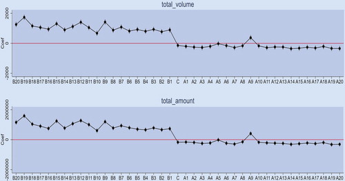
We mentioned before that a critical assumption of the difference-in-difference model is that the Shanghai Stock Exchange and the Shenzhen Stock Exchange should have parallel trends. We have to conduct a parallel trend test and event study to ensure the reliability of our regressions. Results are plotted in Figure 6. It can be seen that the positive difference between treat group and control group is very stable before the introduction of call auction. It fluctuates around a certain positive value. After the introduction of call auction, the difference between them quickly turns to negative and fluctuates around a negative value. We can conclude that there is a strong parallel trend between our treat group and control group. Results derived from difference-in-difference models are relatively reliable.

Figure 6. Parallel trend tests for volume and amount. Notes: The “B” represents before, “C” represents current and “A” represents after. We assume current is August 20, 2018.

We also want to strengthen our causality inference by conducting placebo tests with reference to Li and Tang (2016). Specifically, the samples are sorted by random order each time, and the main variable $treated\mathrm{\_}period$ is randomly assigned. Then it is used as a placebo to test whether there are placebo effects. We carry out 500 times of random simulations. The t statistic of random $treated\mathrm{\_}period$ is calculated each time. As is shown in Table 5, the mean value of t-statistics obtained from 500 random simulations are almost zero, and the standard deviation is significantly greater than the mean value, indicating that there are no placebo effects. This suggests that the difference-in-difference models are robust.

Table 5. Placebo tests for volume and amount.

	total_amount	total_volume
Mean value of t statistic	−0.0546413	−0.058837
Standard deviation of t statistic	0.992429	0.991163
Times of random simulations	500	500
Does placebo have a significant effect	No significant effect on the previous conclusions	No significant effect on the previous conclusions

Notes: This table shows the placebo tests of volume and amount. There seems to be no placebo effects.

As is described before, if the introduction of call auction causes a shift of trading volume from closing call to preceding continuous trading, we could not only observe a reduction of trading volume in last three minutes but also observe an increase of trading volume before the closing call minutes. From Table 6 and Appendix 3, we could see that the coefficients of the difference-in-difference variable $treated\mathrm{\_}period$ is positive and significant at 1% level. This indicates that the introduction of call auction would increase the trading volume in minutes of continuous trading before the closing call. Together with tests conducted previously, we could conclude that the introduction of call auction would result in a shift of trading volume from closing call to preceding continuous auction, which is consistent with Huang and Tsai (2008). This can be caused by investors’ desire to close out their position earlier in order to avoid risks related to order book opaqueness. We also include regressions without variables that could be only found quarterly in order to ensure the robustness of our conclusions. It seems that those financial indicators don not have a material impact on our conclusions.

Table 6. DID tests for volume shift.

	(1)	(2)	(3)	(4)	(5)	(6)
Variables	total_volume_3	total_volume_15	total_volume_30	total_volume_3	total_volume_15	total_volume_30
treated_period	261.9***	483.3***	702.3***	264.9***	462.2***	629.8***
	(15.59)	(57.01)	(97.17)	(15.57)	(56.91)	(96.98)
treated	−115.3***	201.0***	632.3***	−202.8***	−157.2***	−6.900
	(10.99)	(40.20)	(68.50)	(11.02)	(40.29)	(68.66)
period	−74.51***	−170.6***	−351.4***	−61.34***	−157.1***	−372.8***
	(10.48)	(38.34)	(65.33)	(10.58)	(38.68)	(65.91)
ma5	−119.1***	−451.0***	−790.4***	−120.5***	−459.1***	−806.2***
	(4.445)	(16.26)	(27.70)	(4.436)	(16.22)	(27.63)
bbi	11.26**	45.30***	105.0***	43.20***	158.9***	289.8***
	(4.708)	(17.22)	(29.34)	(4.714)	(17.23)	(29.37)
macd	−334.6***	−1,325***	−2,341***	−281.8***	−1,136***	−2,029***
	(19.23)	(70.31)	(119.8)	(19.18)	(70.12)	(119.5)
sar	−57.85***	−214.3***	−363.2***	−62.79***	−229.6***	−385.6***
	(3.939)	(14.40)	(24.55)	(3.933)	(14.38)	(24.50)
beta	28.71***	201.1***	423.0***	30.26***	206.1***	430.3***
	(5.323)	(19.47)	(33.18)	(5.308)	(19.40)	(33.06)
turnover	1,402***	5,251***	8,877***	1,398***	5,243***	8,871***
	(2.518)	(9.210)	(15.70)	(2.517)	(9.202)	(15.68)
dominant_buy_ratio	1,219***	3,563***	6,858***	1,183***	3,423***	6,614***
	(39.81)	(145.6)	(248.1)	(39.70)	(145.1)	(247.3)
pe	2.644***	7.289***	9.558***	2.344***	7.079***	10.28***
	(0.0813)	(0.297)	(0.507)	(0.0884)	(0.323)	(0.551)
market_value	0.00474***	0.0189***	0.0329***	0.00434***	0.0172***	0.0297***
	(8.19e−06)	(3.00e−05)	(5.11e−05)	(1.08e−05)	(3.96e−05)	(6.76e−05)
roa				−106.8***	−428.7***	−746.2***
				(1.423)	(5.203)	(8.867)
eps				−290.8***	−559.1***	−440.7***
				(19.16)	(70.05)	(119.4)
lev				8.533***	33.20***	56.91***
				(0.233)	(0.853)	(1.454)
gross_profit_margin				33.88***	144.4***	259.3***
				(0.524)	(1.915)	(3.264)
operating_profit_growth				0.295***	1.578***	3.100***
				(0.0495)	(0.181)	(0.309)
operating_revenue				8.31e−08***	3.51e−07***	6.48e−07***
				(2.11e−09)	(7.70e−09)	(1.31e−08)
Constant	−1,046***	−4,168***	−7,926***	−1,521***	−6,074***	−11,280***
	(21.60)	(79.00)	(134.6)	(23.66)	(86.50)	(147.4)
Observations	2,436,106	2,436,106	2,436,106	2,436,106	2,436,106	2,436,106
R-squared	0.197	0.216	0.219	0.202	0.221	0.224

Notes: Standard errors in parentheses ***p < 0.01, **p < 0.05, *p < 0.1. Observations represent number of observations in our regression sample.

We choose the asymmetric sample period based on fiscal years from 2017 to 2019. To ensure that our conclusions would not be affected by the sample period, we also construct a symmetric sample of 250 days. The results in Appendix 4 are almost the same as before, so sample change would not influence our conclusions.

4.3. Empirical test results of price fluctuation

Firstly, we plot the time series of $abs$ defined before to observe their variations near the introduction of call auction. The higher those variables are, the greater the extent to which closing price deviates from the average price before closing. It can be seen from Figure 7 that under continuous trading, the price fluctuation of the Shanghai Stock Exchange is almost the same as that of the Shenzhen Stock Exchange. While after the introduction of call auction, the price fluctuation of Shanghai Stock Exchange is significantly lower than that of Shenzhen Stock Exchange, indicating that call auction mechanism helps to reduce the abrupt change of the price near the closing. It could help to achieve the goal of stabilizing the closing price. We could also see a strong parallel trend between the Shanghai Stock Exchange and the Shenzhen Stock Exchange, which enhances the feasibility of our difference-in-difference models.

Figure 7. Time series of absolute price difference of different exchanges. Notes: This figure shows the absolute price difference of last three minutes’ price compared with preceding minutes’ volume weighted price. We could see a clear decrease of Shanghai Stock Exchange after the introduction of closing call.

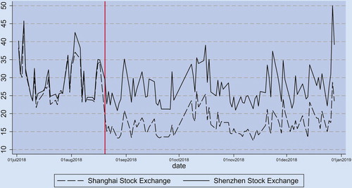
Figure 8. Parallel trend tests for price fluctuation. Notes: The “B” represents before, “C” represents current and “A” represents after. We assume current is August 20, 2018.

Then we will conduct empirical tests mentioned before to test their relationship. We get the regression results in Table 7 using the difference-in-difference models constructed previously. From Table 7, we can see that the coefficients of difference-in-difference variables are all negative and significant at the 1% level. It would, on average, reduce the closing price deviation by approximately 0.05%. The introduction of call auction reduces the price fluctuation near the closing with statistical significance and economic significance.

Table 7. DID tests for price fluctuation.

	(1)	(2)	(3)	(4)	(5)	(6)
Variables	abs_3	nabs_3	abs_15	nabs_15	abs_30	nabs_30
treated_period	−0.00909***	−0.000502***	−0.00161***	−9.28e−05***	−0.00116***	−3.00e−05***
	(9.32e−05)	(3.79e−06)	(0.000186)	(7.10e−06)	(0.000254)	(9.43e−06)
treated	0.00885***	0.000469***	0.00177***	7.52e−05***	0.000607***	5.37e−05***
	(6.60e−05)	(2.68e−06)	(0.000131)	(5.03e−06)	(0.000180)	(6.67e−06)
period	0.00357***	0.000102***	0.00365***	1.48e−05***	0.00311***	7.36e−05***
	(6.33e−05)	(2.58e−06)	(0.000126)	(4.83e−06)	(0.000173)	(6.41e−06)
ma5	0.00119***	2.92e−05***	0.00245***	4.91e−05***	0.00340***	6.30e−05***
	(2.66e−05)	(1.08e−06)	(5.29e−05)	(2.02e−06)	(7.25e−05)	(2.69e−06)
bbi	0.000180***	−3.74e−05***	0.000426***	−6.97e−05***	0.000369***	−0.000103***
	(2.82e−05)	(1.15e−06)	(5.62e−05)	(2.15e−06)	(7.70e−05)	(2.85e−06)
macd	−0.000980***	−0.000127***	−0.000931***	−0.000209***	−0.00249***	−0.000333***
	(0.000115)	(4.67e−06)	(0.000229)	(8.75e−06)	(0.000313)	(1.16e−05)
sar	4.02e−05*	6.36e−06***	0.000181***	2.02e−05***	0.000495***	4.04e−05***
	(2.35e−05)	(9.58e−07)	(4.69e−05)	(1.79e−06)	(6.42e−05)	(2.38e−06)
beta	−0.000435***	−2.90e−05***	−0.000303***	−2.42e−05***	0.000142	1.60e−06
	(3.18e−05)	(1.29e−06)	(6.33e−05)	(2.42e−06)	(8.67e−05)	(3.21e−06)
turnover	0.00106***	6.70e−05***	0.00483***	0.000296***	0.00820***	0.000491***
	(1.51e−05)	(6.13e−07)	(3.00e−05)	(1.15e−06)	(4.11e−05)	(1.52e−06)
dominant_buy_ratio	0.00387***	2.48e−05**	0.00722***	0.000111***	0.00749***	3.13e−06
	(0.000238)	(9.66e−06)	(0.000473)	(1.81e−05)	(0.000648)	(2.40e−05)
pe	1.77e−05***	3.63e−08*	3.99e−05***	2.32e−07***	5.22e−05***	3.38e−07***
	(5.29e−07)	(2.15e−08)	(1.05e−06)	(4.04e−08)	(1.44e−06)	(5.36e−08)
market_value	−1.85e−09***	−9.71e−11***	−5.38e−10***	−0	−3.47e−10*	6.21e−11***
	(6.49e−11)	(0)	(1.29e−10)	(0)	(1.77e−10)	(0)
roa	0.000205***	−7.40e−07**	0.000466***	1.32e−06**	0.000641***	1.96e−06**
	(8.52e−06)	(3.47e−07)	(1.70e−05)	(6.50e−07)	(2.33e−05)	(8.62e−07)
eps	−0.00162***	−0.000193***	−0.00288***	−0.000310***	−0.00416***	−0.000372***
	(0.000115)	(4.67e−06)	(0.000228)	(8.74e−06)	(0.000313)	(1.16e−05)
lev	2.21e−05***	8.18e−07***	5.69e−05***	1.02e−06***	7.99e−05***	9.32e−07***
	(1.40e−06)	(5.68e−08)	(2.78e−06)	(1.06e−07)	(3.81e−06)	(1.41e−07)
gross_profit_margin	−4.25e−05***	−2.89e−06***	−6.37e−05***	−6.17e−06***	−6.00e−05***	−7.61e−06***
	(3.14e−06)	(1.28e−07)	(6.25e−06)	(2.39e−07)	(8.56e−06)	(3.17e−07)
operating_profit_growth	1.18e−06***	2.22e−07***	4.45e−06***	5.56e−07***	6.12e−06***	7.42e−07***
	(2.97e−07)	(1.21e−08)	(5.90e−07)	(2.26e−08)	(8.09e−07)	(3.00e−08)
operating_revenue	−0***	−0***	−0***	−0***	0	−0***
	(0)	(0)	(0)	(0)	(0)	(0)
Constant	−0.0104***	0.00101***	−0.0254***	0.00182***	−0.0369***	0.00237***
	(0.000142)	(5.76e−06)	(0.000282)	(1.08e−05)	(0.000387)	(1.43e−05)
Observations	2,436,106	2,436,106	2,436,106	2,436,106	2,436,106	2,436,106
R-squared	0.158	0.027	0.194	0.040	0.209	0.057

Notes: Standard errors in parentheses ***p < 0.01, **p < 0.05, *p < 0.1. Observations represent number of observations in our regression sample.

As for control variables, the coefficients are consistent with prior research. For example, we find that PE ratio is positively associated with price fluctuation because those with a high PE would be growth stocks. They are fluctuant and risky (Fama and French 2015). The positive relationship between operating profit growth and price fluctuation also tell the same story.

In order to mitigate the unobservable factors of companies and trading days that could cause the endogeneity problem, we control company fixed effects and trading day fixed effects the same as before. The results are shown in Appendix 5. The regression results are almost the same as Table 7. We can see that the coefficients of $treated\mathrm{\_}period$ are still negative and significant at the 1% level. This further demonstrates that the introduction of call auction would significantly reduce the price fluctuation near the closing and stabilize the market.

We choose the sample period of 2017–2019 according to the fiscal year previously, which is not symmetric around the introduction of the closing auction on August 20, 2018. We have to change the window length as well as construct a symmetric sample around August 20, 2018, to ensure the robustness of our findings. Specifically, we choose symmetric windows of 10 days, 20 days, 60 days and 250 days (consistent with previous robustness checks) to test the robustness of our findings. The regression results are shown in Appendix 6. It can be seen that the coefficients of the difference-in-difference variable $treated\mathrm{\_}period$ remain negative and significant at the 1% level. The number of observations is growing with the extension of the window period, which is consistent with intuition. This suggests that our conclusions remain robust in symmetric subsamples of different window length.

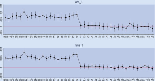
Similar to above, we use event study and parallel trend test to test if the price fluctuation of the Shenzhen Stock Exchange and the Shanghai Stock Exchange have a parallel trend to ensure the robustness of our difference-in-difference models (Figure 8). We can see that the difference between them fluctuates around 0.005 before the introduction of call auction, which suggests a robust parallel trend between them. Their difference quickly decreases to zero after the Shanghai Stock Exchange changing to call auction and remains stable later on. This indicates that the introduction of call auction reduces the price fluctuation of the Shanghai Stock Exchange.

Similar to the above, we use the placebo tests to strengthen our causality inference. By randomly sorting samples and carrying out simulations of 500 times, we get the results in Table 8. The mean value is very close to zero, and the standard deviation is significantly greater than the mean. It indicates that no placebo effects exist. The regression results of the difference-in-difference model are robust.

Table 8. Placebo tests for price fluctuation.

	abs_3	nabs_3
Mean value of t statistic	0.0348547	−0.0137942
Standard deviation of t statistic	1.002226	1.011901
Times of random simulations	500	500
Does placebo have a significant effect	No significant effect on the previous conclusions	No significant effect on the previous conclusions

Notes: This table shows the placebo tests of volume and amount. There seems to be no placebo effects.

We are also curious about the impact of call auction on volatility in minutes of continuous trading preceding the closing call to test whether the introduction of call auction shift liquidity traders to preceding continuous trading. As is mentioned before, we conduct regressions in order to test that the introduction of call auction shift liquidity traders to continuous trading preceding the closing call, thus increasing the volatility before the closing call. The results are shown in Table 9. We can see that the coefficients of the difference-in-difference variable $treated\mathrm{\_}period$ are all positive and significant at the 1% level, which indicates that the introduction of call auction would shift those liquidity traders to preceding continuous trading and increases volatility. This is consistent with the previous findings (Roşu 2009, Chang et al. 2020). We also include regressions without those financial indicators that could only be acquired quarterly. It seems that those variables do not have a material impact on our results. We also control those unobservable company and trading day effects to ensure the robustness of our finds as described before. The results are shown in Appendix 7. It seems that our conclusions remain robust after controlling fixed effects.

Table 9. DID tests for volatility of continuous trading preceding the closing call.

	(1)	(2)	(3)	(4)	(5)	(6)
Variables	volatility_3	volatility_15	volatility_30	volatility_3	volatility_15	volatility_30
treated_period	0.00203***	0.00214***	0.00256***	0.00204***	0.00203***	0.00233***
	(7.54e−05)	(0.000121)	(0.000160)	(7.55e−05)	(0.000121)	(0.000160)
treated	−0.00192***	−0.00160***	−0.00155***	−0.00194***	−0.00170***	−0.00171***
	(5.32e−05)	(8.52e−05)	(0.000113)	(5.34e−05)	(8.57e−05)	(0.000114)
period	0.00199***	0.00303***	0.00390***	0.00206***	0.00312***	0.00393***
	(5.07e−05)	(8.13e−05)	(0.000108)	(5.13e−05)	(8.23e−05)	(0.000109)
ma5	0.00108***	0.00207***	0.00271***	0.00109***	0.00212***	0.00278***
	(2.15e−05)	(3.45e−05)	(4.57e−05)	(2.15e−05)	(3.45e−05)	(4.57e−05)
bbi	4.01e−05*	0.000349***	0.000530***	−6.13e−06	0.000230***	0.000343***
	(2.28e−05)	(3.65e−05)	(4.84e−05)	(2.29e−05)	(3.67e−05)	(4.86e−05)
macd	−0.000526***	−0.000478***	−0.00177***	−0.000514***	−0.000471***	−0.00179***
	(9.30e−05)	(0.000149)	(0.000198)	(9.30e−05)	(0.000149)	(0.000198)
sar	0.000161***	0.000227***	0.000339***	0.000179***	0.000261***	0.000394***
	(1.90e−05)	(3.05e−05)	(4.05e−05)	(1.91e−05)	(3.06e−05)	(4.05e−05)
beta	−0.000488***	−0.000263***	7.80e−05	−0.000483***	−0.000263***	7.56e−05
	(2.57e−05)	(4.13e−05)	(5.47e−05)	(2.57e−05)	(4.13e−05)	(5.47e−05)
turnover	0.000804***	0.00424***	0.00678***	0.000797***	0.00424***	0.00680***
	(1.22e−05)	(1.95e−05)	(2.59e−05)	(1.22e−05)	(1.96e−05)	(2.59e−05)
dominant_buy_ratio	0.00253***	0.00554***	0.00779***	0.00259***	0.00560***	0.00787***
	(0.000192)	(0.000309)	(0.000409)	(0.000192)	(0.000309)	(0.000409)
pe	1.64e−05***	2.95e−05***	3.62e−05***	1.64e−05***	3.18e−05***	4.16e−05***
	(3.93e−07)	(6.30e−07)	(8.36e−07)	(4.29e−07)	(6.87e−07)	(9.11e−07)
market_value	−1.43e−09***	4.56e−10***	2.20e−09***	−1.16e−09***	6.97e−11	1.27e−09***
	(0)	(6.35e−11)	(8.42e−11)	(5.26e−11)	(8.43e−11)	(1.12e−10)
roa				0.000193***	0.000479***	0.000676***
				(6.90e−06)	(1.11e−05)	(1.47e−05)
eps				−0.000666***	−0.00261***	−0.00281***
				(9.29e−05)	(0.000149)	(0.000197)
lev				2.46e−05***	5.15e−05***	6.86e−05***
				(1.13e−06)	(1.81e−06)	(2.41e−06)
gross_profit_margin				−3.77e−05***	−5.67e−05***	−6.93e−05***
				(2.54e−06)	(4.07e−06)	(5.40e−06)
operating_profit_growth				9.92e−07***	2.57e−06***	3.41e−06***
				(2.40e−07)	(3.85e−07)	(5.11e−07)
operating_revenue				−0***	−0	0**
				(0)	(0)	(0)
Constant	−0.00464***	−0.0188***	−0.0294***	−0.00557***	−0.0213***	−0.0329***
	(0.000104)	(0.000168)	(0.000222)	(0.000115)	(0.000184)	(0.000244)
Observations	2,436,104	2,436,104	2,436,105	2,436,104	2,436,104	2,436,105
R-squared	0.178	0.293	0.311	0.179	0.294	0.312

Notes: Standard errors in parentheses ***p < 0.01, **p < 0.05, *p < 0.1. Observations represent number of observations in our regression sample.

There are also concerns that we choose an asymmetric sample according to the fiscal year. So we change our sample period to 250 days, 60 days, 20 days and 10 days consistent with previous tests to ensure the robustness of our conclusions. From the results in Appendix 8, we can see that our conclusions remain robust in different subsamples.

4.4. Empirical test results of market efficiency

We conduct three-stages regressions described previously, and the results are shown in Table 10. We could see that $\widehat{b_{j,period}}$ is negatively associated with the difference-in-difference variable $treated\mathrm{\_}period$ when it is positive. However, it is positively associated with the difference-in-difference variable $treated\mathrm{\_}period$ when it is negative. Both are significant at the 1% level. This indicates that the introduction of call auction would alleviate the overreaction and underreaction, thus improving market efficiency. This could also be observed by the negative relationship between $|\widehat{b_{j,period}}|$ and $treated\mathrm{\_}period$, which indicates that the introduction of call auction would bring $\widehat{b_{j,period}}$ closer to zero. Our conclusions remain robust in different subsamples.

Table 10. Three-stages regressions for market efficiency.

Sample	Variables	$\widehat{b_{j,period}}>0$	$\widehat{b_{j,period}}<0$	$\left|\widehat{b_{j,period}}\right|$
Full Sample (Asymmetric)	treated_period	−0.000903***	0.00125***	−0.00145***
		−0.00031	−0.00043	−0.00037
	treated	0.00138***	−0.00174***	0.00203***
		−0.00023	−0.0003	−0.00026
	period	−0.000808***	0.00185***	−0.00116***
		−0.0002	−0.00028	−0.00023
	Constant	0.00351***	−0.00448***	0.00417***
		−0.00014	−0.00019	−0.00017
	Observations	3,697	3,480	7,177
	R-squared	0.026	0.045	0.022
250 Days (Symmetric)	treated_period	−0.00132***	0.00257*	−0.00108***
		−0.00024	−0.00136	−0.00022
	treated	0.00288***	−0.00376***	0.00290***
		−0.00024	−0.00112	−0.00019
	period	−0.00055	0.00263	−0.000629**
		−0.00036	−0.00181	−0.0003
	Constant	0.00607***	−0.00759***	0.00625***
		−0.00015	−0.00089	−0.00014
	Observations	3,697	3,480	7,177
	R-squared	0.079	0.011	0.064
120 Days (Symmetric)	treated_period	−0.00135***	0.000565*	−0.000956**
		−0.00031	−0.00032	−0.00043
	treated	0.000162	−8.93E−05	0.000159
		−0.00023	−0.00021	−0.00031
	period	−0.00112***	0.00142***	−0.00247***
		−0.00022	−0.00018	−0.00028
	Constant	0.00655***	−0.00775***	0.00956***
		−0.00015	−0.00013	−0.0002
	Observations	3,697	3,480	7,177
	R-squared	0.02	0.03	0.016

Notes: Standard errors in parentheses ***p < 0.01, **p < 0.05, *p < 0.1. Observations represent number of observations in our regression sample.

We also calculate the ratio of open-to-open returns to close-to-close returns in reference to Stoll (2000) to test market efficiency as robustness checks. The results are shown in Appendix 9. We include both the difference-in-difference model and the fixed effects model to ensure the robustness of our tests. We also conduct regressions without those variables that could only be found in quarterly reports the same as previous tests. It seems that the coefficients of $treated\mathrm{\_}period$ are negative and significant at 1% level, which indicates that the call auction results in ratios of open-to-open returns to close-to-close returns closer to 1.0, thus improving the market efficiency.

We also change our sample period to ensure that our regressions would not be influenced by choice of the sample as described previously. The results are shown in Appendix 10. It seems that the length of our sample period or whether it is asymmetric or not would not have a material impact on our conclusions. The coefficients of $treated\mathrm{\_}period$ remain negative and significant.

We also carry out placebo tests the same as before to ensure the robustness of our difference-in-difference models. The mean value of t statistic is −0.0505189, and the standard deviation of t statistic is 0.9714771, which indicates no placebo effects on previous conclusions and our difference-in-difference models are reliable.

5. Conclusions and suggestions

In this paper we study the trading mechanism change in the Shanghai Stock Exchange on August 20, 2018. Using the Shenzhen Stock Exchange as a comparison, we construct difference-in-difference models to identify the causality effects of call auction introduction on trading volume, price volatility and market efficiency. We also conduct robustness checks by testing different subsamples, testing parallel trends and testing placebo effects.

We find that trading volume is significantly lower in the last three minutes after the introduction of a call auction. However, trading volume in the minutes of continuous trading preceding the closing call increases substantially. This indicates a shift of trading volume from the call auction to the preceding continuous trading, which could be explained by liquidity investors’ impatience (Foucault et al. 2005, Roşu 2009), order book opaqueness risks (Huang and Tsai 2008) and lower manipulation (Hillion and Suominen 2004). We also find a decrease of closing price deviation at the closing call, but higher price volatility in the preceding continuous trading. This results in less liquidity noise in closing price formation and improves market efficiency. Our conclusions are robust after changing the sample period, controlling unobservable fixed effects and conducting parallel trend tests and placebo tests.

Our conclusions have important policy implications. We find that the introduction of a call auction would stabilize the closing price formation and improve market efficiency. It would be helpful for developing countries to introduce the closing call to construct a more transparent capital market. We also find that manipulation plays a vital role in disturbing the market, which suggests that regulators should enhance supervision for the manipulators.

Some further studies could be done on this issue. As Twu and Wang (2018) indicate, the time interval or frequency of call auction can also impact market efficiency. Three minutes of call auction in the Chinese market now is quite subjective. Further theoretical studies are needed to determine the optimal time interval for a call auction to achieve the goal of building an efficient capital market.

Acknowledgments

We thank the anonymous reviewers of this journal for their helpful comments.

Disclosure statement

No potential conflict of interest was reported by the authors.

Additional information

Funding

This work was supported by National Natural Science Foundation of China: [grant numbers 71573050, 71573170].

Appendix 1

Fixed effects test for volume and amount

Table

	(1)	(2)	(3)	(4)	(5)	(6)
Variables	total_volume	total_amount	total_volume	total_amount	total_volume	total_amount
treated_period	−1,890***	−1.911e+06***	−1,437***	−1.578e+06***	−1,391***	−1.529e+06***
	(12.32)	(13,659)	(11.92)	(13,084)	(11.96)	(13,129)
ma5			−43.24***	75,456***	−47.01***	73,214***
			(3.393)	(3,724)	(3.394)	(3,725)
bbi			29.41***	88,266***	39.95***	88,395***
			(3.681)	(4,040)	(3.702)	(4,063)
macd			93.41***	516,740***	116.6***	548,107***
			(16.92)	(18,574)	(16.93)	(18,586)
sar			−56.18***	−101,890***	−55.51***	−95,911***
			(3.053)	(3,350)	(3.059)	(3,358)
beta			69.68***	86,304***	70.56***	86,962***
			(4.561)	(5,006)	(4.560)	(5,006)
turnover			1,008***	1.094e+06***	1,001***	1.088e+06***
			(2.504)	(2,749)	(2.508)	(2,753)
dominant_buy_ratio			1,427***	1.498e+06***	1,417***	1.507e+06***
			(33.31)	(36,560)	(33.30)	(36,556)
pe			1.850***	4,865***	2.065***	5,075***
			(0.0841)	(92.30)	(0.0860)	(94.45)
market_value			0.00332***	4.311***	0.00337***	4.308***
			(1.83e−05)	(0.0201)	(1.85e−05)	(0.0203)
roa					−21.31***	4,150*
					(1.989)	(2,183)
eps					−54.82***	162,449***
					(19.57)	(21,482)
lev					5.808***	14,371***
					(0.473)	(519.3)
gross_profit_margin					−5.805***	−10,675***
					(0.806)	(884.2)
operating_profit_growth					0.337***	473.6***
					(0.0455)	(49.95)
operating_revenue					−1.44e−07***	−0.000149***
					(5.07e−09)	(5.56e−06)
Constant	2,357***	2.591e+06***	−1,342***	−3.877e+06***	−1,125***	−4.043e+06***
	(3.858)	(4,276)	(21.17)	(23,239)	(33.08)	(36,308)
Company Fixed Effects	Controlled	Controlled	Controlled	Controlled	Controlled	Controlled
Day Fixed Effects	Controlled	Controlled	Controlled	Controlled	Controlled	Controlled
Observations	2,436,106	2,436,106	2,436,106	2,436,106	2,436,106	2,436,106
R-squared	0.326	0.313	0.379	0.379	0.379	0.380

Notes: Standard errors in parentheses ***p < 0.01, **p < 0.05, *p < 0.1. Observations represent number of observations in our regression sample.

Appendix 2. Robustness checks of different window for volume and amount

Table

Window length	10	10	20	20	60	60	250	250
Variables	total_volume	total_amount	total_volume	total_amount	total_volume	total_amount	total_volume	total_amount
treated_period	−1,098***	−935,921***	−1,074***	−926,705***	−882.0***	−759,565***	−913.3***	−953,820***
	(56.43)	(58,109)	(45.18)	(45,965)	(26.25)	(25,802)	(15.78)	(15,910)
treated	1,012***	874,308***	1,024***	899,891***	758.5***	697,252***	881.5***	927,651***
	(40.69)	(41,900)	(32.52)	(33,093)	(18.79)	(18,474)	(11.44)	(11,538)
period	15.47	37,561	15.83	45,031	233.7***	251,199***	137.8***	240,459***
	(36.55)	(37,637)	(29.54)	(30,058)	(17.16)	(16,872)	(10.51)	(10,599)
ma5	285.7***	765,433***	136.1***	419,499***	33.85***	239,131***	−89.45***	42,110***
	(44.91)	(46,248)	(24.77)	(25,207)	(12.71)	(12,491)	(6.859)	(6,915)
bbi	−314.3***	−427,971***	−145.8***	−140,922***	−83.42***	−83,955***	−5.964	53,203***
	(47.85)	(49,273)	(24.39)	(24,815)	(12.61)	(12,398)	(7.029)	(7,087)
macd	−179.5	−1.083e+06***	333.2***	−237,798***	−515.3***	−781,514***	−344.2***	−293,766***
	(120.7)	(124,291)	(84.83)	(86,312)	(39.96)	(39,282)	(20.93)	(21,100)
sar	−62.64***	−287,366***	−87.05***	−224,329***	−43.31***	−108,933***	−0.796	−53,909***
	(22.68)	(23,357)	(17.04)	(17,339)	(9.155)	(9,000)	(4.698)	(4,736)
beta	−238.6***	31,834	−314.1***	1,144	−281.9***	−73,757***	−180.3***	48,792***
	(35.48)	(36,529)	(27.80)	(28,291)	(15.43)	(15,168)	(7.589)	(7,651)
turnover	1,286***	1.142e+06***	1,292***	1.113e+06***	1,113***	977,938***	969.7***	879,690***
	(16.71)	(17,209)	(12.57)	(12,788)	(6.722)	(6,608)	(3.231)	(3,257)
dominant_buy_ratio	394.9***	694,594***	527.5***	622,451***	619.2***	619,459***	700.7***	846,963***
	(148.3)	(152,695)	(111.8)	(113,730)	(65.34)	(64,238)	(40.61)	(40,939)
pe	0.218	2,497***	0.273	2,986***	−0.0131	2,614***	1.904***	3,955***
	(0.501)	(516.0)	(0.402)	(408.8)	(0.230)	(226.6)	(0.128)	(129.3)
market_value	0.00261***	2.559***	0.00282***	2.737***	0.00257***	2.560***	0.00290***	3.097***
	(5.25e−05)	(0.0540)	(4.17e−05)	(0.0425)	(2.40e−05)	(0.0236)	(1.33e−05)	(0.0134)
roa	−36.27***	−33,590***	−51.07***	−45,518***	−44.58***	−38,706***	−62.27***	−58,286***
	(5.399)	(5,559)	(4.307)	(4,382)	(2.490)	(2,448)	(1.485)	(1,497)
eps	−172.0*	−274,630***	−88.06	−193,994**	−42.99	−161,090***	−49.41**	−1,733
	(94.60)	(97,410)	(76.93)	(78,272)	(45.28)	(44,510)	(19.77)	(19,929)
lev	5.383***	6,007***	7.045***	6,985***	7.885***	7,385***	8.856***	8,925***
	(0.878)	(904.0)	(0.701)	(713.5)	(0.406)	(399.3)	(0.243)	(244.8)
gross_profit_margin	8.626***	8,934***	15.03***	14,369***	14.79***	13,425***	23.45***	19,749***
	(1.969)	(2,027)	(1.573)	(1,600)	(0.911)	(895.3)	(0.539)	(543.7)
operating_profit_growth	0.833***	1,363***	0.823***	1,227***	0.409***	870.2***	0.0409	517.8***
	(0.174)	(179.4)	(0.139)	(141.8)	(0.0811)	(79.68)	(0.0493)	(49.70)
operating_revenue	1.60e−08*	4.57e−05***	2.76e−08***	6.60e−05***	1.66e−08***	5.09e−05***	2.16e−08***	3.54e−05***
	(8.23e−09)	(8.48e−06)	(6.55e−09)	(6.66e−06)	(3.77e−09)	(3.70e−06)	(2.20e−09)	(2.22e−06)
Constant	−632.2***	−2.635e+06***	−781.4***	−2.848e+06***	−782.3***	−2.645e+06***	−1,091***	−3.226e+06***
	(86.26)	(88,820)	(69.16)	(70,374)	(41.01)	(40,316)	(25.26)	(25,462)
Observations	34,171	34,171	68,366	68,366	201,405	201,405	823,457	823,457
R-squared	0.254	0.264	0.240	0.242	0.206	0.221	0.186	0.204

Notes: Standard errors in parentheses ***p < 0.01, **p < 0.05, *p < 0.1. Observations represent number of observations in our regression sample.

Appendix 3. DID tests for amount shift

Table

	(1)	(2)	(3)	(4)	(5)	(6)
Variables	total_amount_3	total_amount_15	total_amount_30	total_amount_3	total_amount_15	total_amount_30
treated_period	384,731***	774,885***	1.087e+06***	381,856***	737,136***	993,300***
	(15,145)	(56,866)	(95,542)	(15,122)	(56,752)	(95,318)
treated	−268,550***	−288,894***	−184,689***	−369,915***	−718,287***	−954,623***
	(10,678)	(40,091)	(67,359)	(10,706)	(40,181)	(67,487)
period	156,061***	1.023e+06***	1.898e+06***	158,149***	954,249***	1.713e+06***
	(10,183)	(38,236)	(64,241)	(10,278)	(38,574)	(64,787)
ma5	61,564***	233,742***	354,989***	57,310***	210,524***	310,004***
	(4,318)	(16,214)	(27,241)	(4,309)	(16,171)	(27,161)
Bbi	61,245***	237,095***	434,525***	83,588***	310,972***	550,345***
	(4,574)	(17,173)	(28,852)	(4,579)	(17,185)	(28,864)
macd	93,968***	398,145***	597,105***	143,980***	582,531***	904,879***
	(18,677)	(70,126)	(117,821)	(18,631)	(69,921)	(117,437)
sar	−103,671***	−370,936***	−602,350***	−103,115***	−360,809***	−578,458***
	(3,826)	(14,366)	(24,138)	(3,820)	(14,337)	(24,080)
beta	187,158***	861,180***	1.590e+06***	189,890***	871,703***	1.608e+06***
	(5,171)	(19,416)	(32,621)	(5,156)	(19,349)	(32,498)
turnover	1.402e+06***	5.189e+06***	8.685e+06***	1.400e+06***	5.191e+06***	8.695e+06***
	(2,446)	(9,186)	(15,433)	(2,445)	(9,177)	(15,413)
dominant_buy_ratio	1.599e+06***	5.235e+06***	9.653e+06***	1.573e+06***	5.141e+06***	9.493e+06***
	(38,669)	(145,191)	(243,939)	(38,556)	(144,703)	(243,038)
pe	5,152***	15,678***	22,772***	5,204***	17,457***	27,215***
	(78.95)	(296.4)	(498.0)	(85.90)	(322.4)	(541.5)
market_value	5.472***	22.00***	38.30***	5.050***	20.13***	34.83***
	(0.00796)	(0.0299)	(0.0502)	(0.0105)	(0.0395)	(0.0664)
roa				−98,796***	−392,603***	−682,159***
				(1,383)	(5,189)	(8,715)
eps				136,703***	1.471e+06***	3.293e+06***
				(18,612)	(69,853)	(117,322)
lev				11,743***	45,833***	78,496***
				(226.7)	(850.7)	(1,429)
gross_profit_margin				32,446***	129,876***	227,312***
				(508.9)	(1,910)	(3,208)
operating_profit_growth				906.0***	3,313***	5,673***
				(48.12)	(180.6)	(303.3)
operating_revenue				6.37e−05***	0.000283***	0.000530***
				(2.04e−06)	(7.67e−06)	(1.29e−05)
Constant	−4.352e+06***	−1.724e+07***	−3.028e+07***	−4.933e+06***	−1.955e+07***	−3.431e+07***
	(20,986)	(78,797)	(132,389)	(22,984)	(86,261)	(144,880)
Observations	2,436,106	2,436,106	2,436,106	2,436,106	2,436,106	2,436,106
R-squared	0.234	0.248	0.257	0.239	0.254	0.263

Notes: Standard errors in parentheses ***p < 0.01, **p < 0.05, *p < 0.1. Observations represent number of observations in our regression sample.

Appendix 4. Robustness checks of different window for volume and amount shift

Table

	(1)	(2)	(3)	(4)	(5)	(6)
Variables	total_volume_3	total_amount_3	total_volume_15	total_amount_15	total_volume_30	total_amount_30
treated_period	167.4***	227,234***	256.4***	371,906***	276.5**	399,983***
	(19.28)	(18,479)	(70.52)	(68,758)	(123.1)	(118,762)
treated	−183.7***	−242,138***	−271.3***	−483,906***	−218.5**	−599,590***
	(13.98)	(13,401)	(51.14)	(49,863)	(89.26)	(86,125)
period	143.1***	141,153***	435.9***	593,266***	709.6***	1.118e+06***
	(12.85)	(12,310)	(46.98)	(45,803)	(82.00)	(79,113)
ma5	−125.9***	60,137***	−477.6***	222,202***	−830.1***	366,879***
	(8.381)	(8,031)	(30.65)	(29,883)	(53.50)	(51,615)
bbi	−4.301	75,433***	−11.58	279,021***	6.004	503,680***
	(8.590)	(8,231)	(31.41)	(30,627)	(54.83)	(52,901)
macd	−418.7***	−324,582***	−1,643***	−1.233e+06***	−2,874***	−2.307e+06***
	(25.57)	(24,508)	(93.52)	(91,189)	(163.2)	(157,505)
sar	−4.145	−81,961***	−12.92	−275,865***	−25.80	−466,834***
	(5.740)	(5,501)	(20.99)	(20,468)	(36.64)	(35,353)
beta	−196.4***	83,434***	−501.8***	641,619***	−609.9***	1.381e+06***
	(9.273)	(8,886)	(33.91)	(33,063)	(59.19)	(57,108)
turnover	1,400***	1.255e+06***	5,152***	4.566e+06***	8,689***	7.645e+06***
	(3.948)	(3,783)	(14.44)	(14,077)	(25.20)	(24,315)
dominant_buy_ratio	655.4***	867,515***	1,713***	2.832e+06***	3,159***	4.974e+06***
	(49.62)	(47,550)	(181.5)	(176,925)	(316.7)	(305,591)
pe	1.693***	4,870***	4.687***	16,745***	5.325***	25,629***
	(0.157)	(150.2)	(0.573)	(559.0)	(1.001)	(965.5)
market_value	0.00405***	4.322***	0.0159***	17.37***	0.0275***	30.44***
	(1.62e−05)	(0.0156)	(5.94e−05)	(0.0579)	(0.000104)	(0.100)
roa	−66.22***	−61,637***	−267.2***	−234,558***	−482.8***	−414,740***
	(1.814)	(1,738)	(6.634)	(6,469)	(11.58)	(11,173)
eps	−326.3***	−248,203***	−893.1***	−461,476***	−1,272***	−495,322***
	(24.16)	(23,148)	(88.33)	(86,128)	(154.2)	(148,763)
lev	10.58***	10,591***	38.85***	39,634***	66.23***	68,172***
	(0.297)	(284.3)	(1.085)	(1,058)	(1.894)	(1,827)
gross_profit_margin	24.44***	22,552***	106.1***	86,846***	202.7***	157,611***
	(0.659)	(631.5)	(2.410)	(2,350)	(4.206)	(4,059)
operating_profit_growth	0.0947	780.5***	0.669***	2,775***	1.248***	4,622***
	(0.0602)	(57.73)	(0.220)	(214.8)	(0.385)	(371.0)
operating_revenue	4.22e−08***	5.11e−05***	2.04e−07***	0.000227***	4.10e−07***	0.000426***
	(2.69e−09)	(2.57e−06)	(9.82e−09)	(9.58e−06)	(1.71e−08)	(1.65e−05)
Constant	−1,046***	−3.843e+06***	−4,201***	−1.533e+07***	−7,991***	−2.713e+07***
	(30.86)	(29,574)	(112.9)	(110,039)	(197.0)	(190,064)
Observations	823,457	823,457	823,457	823,457	823,457	823,457
R-squared	0.221	0.252	0.237	0.272	0.233	0.275

Notes: Standard errors in parentheses ***p < 0.01, **p < 0.05, *p < 0.1. Observations represent number of observations in our regression sample.

Appendix 5. Fixed effects tests for price fluctuation

Table

	(1)	(2)	(3)	(4)	(5)	(6)
Variables	abs_3	nabs_3	abs_15	nabs_15	abs_30	nabs_30
treated_period	−0.00867***	−0.000496***	−3.69e−05	−6.89e−05***	−0.00322***	−5.53e−05***
	(9.04e−05)	(3.77e−06)	(0.000177)	(6.96e−06)	(0.000240)	(9.11e−06)
ma5	0.00121***	2.62e−05***	0.00261***	4.33e−05***	0.00370***	5.57e−05***
	(2.57e−05)	(1.07e−06)	(5.02e−05)	(1.98e−06)	(6.82e−05)	(2.58e−06)
bbi	0.000507***	−8.79e−06***	0.000988***	−8.18e−06***	0.00128***	−9.55e−06***
	(2.80e−05)	(1.17e−06)	(5.47e−05)	(2.15e−06)	(7.44e−05)	(2.82e−06)
macd	0.00328***	0.000146***	0.00879***	0.000366***	0.0116***	0.000490***
	(0.000128)	(5.33e−06)	(0.000250)	(9.86e−06)	(0.000340)	(1.29e−05)
sar	−0.000149***	−8.59e−06***	−0.000264***	−2.09e−05***	−0.000250***	−2.82e−05***
	(2.31e−05)	(9.63e−07)	(4.52e−05)	(1.78e−06)	(6.15e−05)	(2.33e−06)
beta	−0.000327***	−2.22e−05***	−0.000102	−1.53e−05***	0.000368***	8.99e−06***
	(3.45e−05)	(1.44e−06)	(6.74e−05)	(2.65e−06)	(9.17e−05)	(3.47e−06)
turnover	0.00168***	0.000101***	0.00575***	0.000347***	0.00911***	0.000539***
	(1.90e−05)	(7.90e−07)	(3.71e−05)	(1.46e−06)	(5.04e−05)	(1.91e−06)
dominant_buy_ratio	0.00992***	0.000434***	0.0250***	0.00127***	0.0372***	0.00192***
	(0.000252)	(1.05e−05)	(0.000492)	(1.94e−05)	(0.000670)	(2.54e−05)
pe	2.87e−05***	6.60e−07***	5.76e−05***	1.28e−06***	7.11e−05***	1.53e−06***
	(6.50e−07)	(2.71e−08)	(1.27e−06)	(5.01e−08)	(1.73e−06)	(6.55e−08)
market_value	2.48e−09***	1.54e−10***	7.25e−09***	6.06e−10***	7.36e−09***	8.28e−10***
	(1.40e−10)	(0)	(2.74e−10)	(0)	(3.72e−10)	(0)
roa	−3.00e−05**	−1.07e−05***	0.000104***	−1.67e−05***	0.000399***	−1.43e−05***
	(1.50e−05)	(6.26e−07)	(2.94e−05)	(1.16e−06)	(4.00e−05)	(1.51e−06)
eps	−0.000881***	−0.000110***	0.000370	−0.000197***	0.000253	−0.000283***
	(0.000148)	(6.16e−06)	(0.000289)	(1.14e−05)	(0.000393)	(1.49e−05)
lev	5.85e−06	1.05e−06***	5.98e−05***	9.05e−07***	0.000132***	1.25e−06***
	(3.58e−06)	(1.49e−07)	(6.99e−06)	(2.75e−07)	(9.51e−06)	(3.60e−07)
gross_profit_margin	−5.62e−05***	6.62e−07***	−0.000158***	7.98e−07*	−0.000270***	−2.06e−07
	(6.09e−06)	(2.54e−07)	(1.19e−05)	(4.69e−07)	(1.62e−05)	(6.13e−07)
operating_profit_growth	−7.60e−07**	−2.87e−08**	−1.27e−06*	−7.62e−08***	−2.49e−06***	−1.41e−07***
	(3.44e−07)	(1.43e−08)	(6.73e−07)	(2.65e−08)	(9.15e−07)	(3.47e−08)
operating_revenue	0***	−0***	0*	−0***	0	−0***
	(0)	(0)	(0)	(0)	(0)	(0)
Constant	−0.0137***	0.000664***	−0.0417***	0.000613***	−0.0638***	0.000556***
	(0.000250)	(1.04e−05)	(0.000489)	(1.93e−05)	(0.000665)	(2.52e−05)
Company Fixed Effects	Controlled	Controlled	Controlled	Controlled	Controlled	Controlled
Day Fixed Effects	Controlled	Controlled	Controlled	Controlled	Controlled	Controlled
Observations	2,436,106	2,436,106	2,436,106	2,436,106	2,436,106	2,436,106
R-squared	0.240	0.079	0.298	0.116	0.322	0.157

Notes: Standard errors in parentheses ***p < 0.01, **p < 0.05, *p < 0.1. Observations represent number of observations in our regression sample.

Appendix 6. Robustness checks of different window for price fluctuation

Table

Window Length	10	10	20	20	60	60	250	250
Variables	abs_3	nabs_3	abs_3	nabs_3	abs_3	nabs_3	abs_3	nabs_3
treated_period	−0.00692***	−0.000541***	−0.00722***	−0.000535***	−0.00748***	−0.000530***	−0.00811***	−0.000496***
	(0.000601)	(3.33e−05)	(0.000433)	(2.40e−05)	(0.000246)	(1.31e−05)	(0.000144)	(6.84e−06)
treated	0.00678***	0.000493***	0.00631***	0.000459***	0.00651***	0.000443***	0.00767***	0.000451***
	(0.000433)	(2.40e−05)	(0.000312)	(1.73e−05)	(0.000176)	(9.36e−06)	(0.000105)	(4.96e−06)
period	−0.00170***	−0.000130***	−0.00131***	−0.000127***	−0.000267*	−3.46e−05***	0.00154***	4.62e−05***
	(0.000389)	(2.15e−05)	(0.000283)	(1.57e−05)	(0.000161)	(8.55e−06)	(9.61e−05)	(4.55e−06)
ma5	0.00498***	0.000151***	0.00305***	0.000110***	0.00249***	6.83e−05***	0.00185***	5.63e−05***
	(0.000478)	(2.65e−05)	(0.000238)	(1.32e−05)	(0.000119)	(6.33e−06)	(6.27e−05)	(2.97e−06)
bbi	−0.00281***	−0.000119***	−0.00140***	−9.16e−05***	−0.00103***	−8.88e−05***	−0.000344***	−6.50e−05***
	(0.000509)	(2.82e−05)	(0.000234)	(1.29e−05)	(0.000118)	(6.28e−06)	(6.43e−05)	(3.04e−06)
macd	−0.00260**	1.80e−05	−0.00128	0.000104**	−0.00327***	−4.96e−05**	−0.00294***	−0.000223***
	(0.00128)	(7.12e−05)	(0.000814)	(4.50e−05)	(0.000375)	(1.99e−05)	(0.000191)	(9.06e−06)
sar	−0.000704***	−3.53e−05***	−0.000191	−2.12e−05**	−3.20e−05	1.51e−05***	3.52e−05	6.50e−06***
	(0.000241)	(1.34e−05)	(0.000163)	(9.05e−06)	(8.58e−05)	(4.56e−06)	(4.30e−05)	(2.03e−06)
beta	−0.00219***	−0.000190***	−0.00221***	−0.000176***	−0.00219***	−0.000150***	−0.00106***	−6.08e−05***
	(0.000378)	(2.09e−05)	(0.000267)	(1.48e−05)	(0.000145)	(7.68e−06)	(6.94e−05)	(3.29e−06)
turnover	0.000919***	9.26e−05***	0.000498***	7.32e−05***	0.000777***	7.07e−05***	0.000723***	6.04e−05***
	(0.000178)	(9.85e−06)	(0.000121)	(6.67e−06)	(6.30e−05)	(3.35e−06)	(2.95e−05)	(1.40e−06)
dominant_buy_ratio	0.00106	−9.60e−05	−0.00436***	−0.000390***	−0.00271***	−0.000302***	0.000806**	−0.000151***
	(0.00158)	(8.74e−05)	(0.00107)	(5.93e−05)	(0.000613)	(3.25e−05)	(0.000371)	(1.76e−05)
pe	2.19e−05***	3.26e−07	2.78e−05***	5.90e−07***	2.64e−05***	4.20e−07***	2.71e−05***	3.01e−07***
	(5.33e−06)	(2.95e−07)	(3.85e−06)	(2.13e−07)	(2.16e−06)	(1.15e−07)	(1.17e−06)	(5.56e−08)
market_value	−5.95e−10	−0	−1.43e−10	−5.20e−11**	−6.76e−10***	−8.07e−11***	−2.13e−09***	−1.27e−10***
	(5.58e−10)	(0)	(4.00e−10)	(0)	(2.25e−10)	(0)	(1.22e−10)	(0)
roa	0.000432***	6.81e−06**	0.000469***	7.00e−06***	0.000447***	7.59e−06***	0.000341***	5.13e−06***
	(5.75e−05)	(3.18e−06)	(4.13e−05)	(2.29e−06)	(2.33e−05)	(1.24e−06)	(1.36e−05)	(6.43e−07)
eps	−0.00109	−4.09e−05	−0.000416	−2.43e−05	−0.00200***	−5.83e−05***	−0.00271***	−0.000218***
	(0.00101)	(5.58e−05)	(0.000738)	(4.08e−05)	(0.000424)	(2.25e−05)	(0.000181)	(8.56e−06)
lev	4.61e−05***	1.99e−06***	4.52e−05***	2.05e−06***	4.63e−05***	2.03e−06***	3.81e−05***	1.58e−06***
	(9.35e−06)	(5.18e−07)	(6.73e−06)	(3.72e−07)	(3.81e−06)	(2.02e−07)	(2.22e−06)	(1.05e−07)
gross_profit_margin	−0.000102***	−6.99e−06***	−0.000117***	−6.91e−06***	−9.47e−05***	−6.36e−06***	−6.45e−05***	−4.23e−06***
	(2.10e−05)	(1.16e−06)	(1.51e−05)	(8.35e−07)	(8.54e−06)	(4.54e−07)	(4.93e−06)	(2.34e−07)
operating_profit_growth	−1.67e−06	1.31e−07	−2.28e−06*	1.09e−07	−1.09e−06	1.12e−07***	−4.62e−07	9.15e−08***
	(1.85e−06)	(1.03e−07)	(1.34e−06)	(7.40e−08)	(7.60e−07)	(4.04e−08)	(4.51e−07)	(2.14e−08)
operating_revenue	−0***	−0***	−0***	−0***	−0***	−0***	−0***	−0***
	(0)	(0)	(0)	(0)	(0)	(0)	(0)	(0)
Constant	−0.00389***	0.00141***	−0.00193***	0.00151***	−0.00338***	0.00140***	−0.00728***	0.00127***
	(0.000918)	(5.08e−05)	(0.000663)	(3.67e−05)	(0.000384)	(2.04e−05)	(0.000231)	(1.09e−05)
Observations	34,171	34,171	68,366	68,366	201,405	201,405	823,457	823,457
R-squared	0.174	0.039	0.168	0.034	0.177	0.032	0.174	0.026

Notes: Standard errors in parentheses ***p < 0.01, **p < 0.05, *p < 0.1. Observations represent number of observations in our regression sample.

Appendix 7. Fixed effects tests for volatility of continuous trading preceding the closing call

Table

	(1)	(2)	(3)	(4)	(5)	(6)
Variables	volatility_3	volatility_15	volatility_30	volatility_3	volatility_15	volatility_30
treated_period	0.00276***	0.00340***	0.00406***	0.00286***	0.00362***	0.00435***
	(7.24e−05)	(0.000108)	(0.000141)	(7.26e−05)	(0.000109)	(0.000142)
ma5	0.00113***	0.00227***	0.00300***	0.00113***	0.00227***	0.00300***
	(2.06e−05)	(3.08e−05)	(4.02e−05)	(2.06e−05)	(3.08e−05)	(4.02e−05)
bbi	0.000104***	0.000567***	0.000845***	0.000124***	0.000550***	0.000773***
	(2.23e−05)	(3.34e−05)	(4.36e−05)	(2.25e−05)	(3.36e−05)	(4.38e−05)
macd	0.00267***	0.00703***	0.00870***	0.00272***	0.00720***	0.00896***
	(0.000103)	(0.000154)	(0.000200)	(0.000103)	(0.000154)	(0.000201)
sar	7.28e−06	−0.000120***	−0.000150***	1.18e−05	−8.36e−05***	−7.80e−05**
	(1.85e−05)	(2.77e−05)	(3.61e−05)	(1.86e−05)	(2.78e−05)	(3.62e−05)
beta	−0.000312***	−7.33e−05*	0.000226***	−0.000310***	−6.48e−05	0.000237***
	(2.77e−05)	(4.14e−05)	(5.40e−05)	(2.77e−05)	(4.14e−05)	(5.40e−05)
turnover	0.00133***	0.00500***	0.00766***	0.00132***	0.00497***	0.00762***
	(1.52e−05)	(2.27e−05)	(2.97e−05)	(1.52e−05)	(2.28e−05)	(2.97e−05)
dominant_buy_ratio	0.00821***	0.0204***	0.0296***	0.00817***	0.0204***	0.0298***
	(0.000202)	(0.000303)	(0.000394)	(0.000202)	(0.000303)	(0.000394)
pe	2.43e−05***	4.19e−05***	5.18e−05***	2.64e−05***	4.56e−05***	5.68e−05***
	(5.10e−07)	(7.64e−07)	(9.96e−07)	(5.22e−07)	(7.82e−07)	(1.02e−06)
market_value	4.64e−09***	5.99e−09***	6.63e−09***	4.98e−09***	6.39e−09***	6.92e−09***
	(1.11e−10)	(1.66e−10)	(2.17e−10)	(1.12e−10)	(1.68e−10)	(2.19e−10)
roa				−3.32e−05***	0.000177***	0.000418***
				(1.21e−05)	(1.81e−05)	(2.36e−05)
eps				−3.51e−05	−0.000194	0.000397*
				(0.000119)	(0.000178)	(0.000232)
lev				1.41e−05***	6.79e−05***	0.000118***
				(2.87e−06)	(4.30e−06)	(5.60e−06)
gross_profit_margin				−5.44e−05***	−0.000150***	−0.000244***
				(4.89e−06)	(7.32e−06)	(9.54e−06)
operating_profit_growth				−5.50e−07**	−1.43e−06***	−1.97e−06***
				(2.76e−07)	(4.13e−07)	(5.39e−07)
operating_revenue				0***	0***	0**
				(0)	(0)	(0)
Constant	−0.0119***	−0.0316***	−0.0452***	−0.0128***	−0.0348***	−0.0507***
	(0.000129)	(0.000192)	(0.000251)	(0.000201)	(0.000301)	(0.000392)
Company Fixed Effects	Controlled	Controlled	Controlled	Controlled	Controlled	Controlled
Day Fixed Effects	Controlled	Controlled	Controlled	Controlled	Controlled	Controlled
Observations	2,436,104	2,436,104	2,436,105	2,436,104	2,436,104	2,436,105
R-squared	0.271	0.454	0.486	0.271	0.454	0.486

Notes: Standard errors in parentheses ***p < 0.01, **p < 0.05, *p < 0.1. Observations represent number of observations in our regression sample.

Appendix 8. Robustness checks of different window for volatility of continuous trading preceding the closing call

Table

Window Length	10	10	10	20	20	20	60	60	60	250	250	250
Variables	volatility_3	volatility_15	volatility_30	volatility_3	volatility_15	volatility_30	volatility_3	volatility_15	volatility_30	volatility_3	volatility_15	volatility_30
treated_period	0.00210***	0.00172**	0.00147	0.000986***	0.000934*	0.00122*	0.00134***	0.000919***	0.000880**	0.00208***	0.00215***	0.00228***
	(0.000454)	(0.000676)	(0.000956)	(0.000343)	(0.000502)	(0.000716)	(0.000202)	(0.000315)	(0.000423)	(0.000116)	(0.000183)	(0.000243)
treated	−0.00194***	−0.00162***	−0.00130*	−0.00155***	−0.00144***	−0.00157***	−0.00193***	−0.00137***	−0.00117***	−0.00217***	−0.00207***	−0.00215***
	(0.000327)	(0.000488)	(0.000689)	(0.000247)	(0.000361)	(0.000516)	(0.000145)	(0.000225)	(0.000303)	(8.44e−05)	(0.000133)	(0.000176)
period	−0.00233***	−0.00413***	−0.00221***	−0.00185***	−0.00475***	−0.00384***	−0.00136***	−0.00314***	−0.00281***	0.000179**	−0.000277**	5.47e−05
	(0.000294)	(0.000438)	(0.000619)	(0.000224)	(0.000328)	(0.000468)	(0.000132)	(0.000206)	(0.000277)	(7.76e−05)	(0.000122)	(0.000162)
ma5	0.00407***	0.0102***	0.0143***	0.00255***	0.00513***	0.00740***	0.00209***	0.00441***	0.00568***	0.00155***	0.00289***	0.00390***
	(0.000361)	(0.000538)	(0.000761)	(0.000188)	(0.000275)	(0.000393)	(9.78e−05)	(0.000152)	(0.000205)	(5.06e−05)	(7.98e−05)	(0.000106)
bbi	−0.00261***	−0.00685***	−0.00993***	−0.00142***	−0.00266***	−0.00438***	−0.000795***	−0.00136***	−0.00177***	−0.000317***	−0.000178**	−0.000530***
	(0.000385)	(0.000573)	(0.000810)	(0.000185)	(0.000271)	(0.000387)	(9.71e−05)	(0.000151)	(0.000203)	(5.19e−05)	(8.18e−05)	(0.000108)
macd	−0.000690	−0.00388***	−0.00878***	0.00107*	−0.00626***	−0.0104***	−0.00213***	−0.00980***	−0.0173***	−0.00170***	−0.00458***	−0.00578***
	(0.000971)	(0.00145)	(0.00204)	(0.000644)	(0.000942)	(0.00134)	(0.000308)	(0.000479)	(0.000645)	(0.000154)	(0.000243)	(0.000322)
sar	−0.000108	−0.000592**	−0.000667*	0.000226*	0.000267	0.000705***	4.15e−05	−0.000354***	−0.000266*	0.000158***	0.000142***	0.000500***
	(0.000183)	(0.000272)	(0.000384)	(0.000129)	(0.000189)	(0.000270)	(7.05e−05)	(0.000110)	(0.000148)	(3.47e−05)	(5.46e−05)	(7.23e−05)
beta	−0.00129***	6.44e−05	0.00143**	−0.00147***	−0.000411	0.000665	−0.00141***	−0.00146***	−0.000738***	−0.00105***	−0.000599***	−5.96e−05
	(0.000285)	(0.000425)	(0.000601)	(0.000211)	(0.000309)	(0.000441)	(0.000119)	(0.000185)	(0.000249)	(5.60e−05)	(8.82e−05)	(0.000117)
turnover	0.000127	0.00420***	0.00686***	−8.06e−05	0.00345***	0.00600***	0.000145***	0.00369***	0.00634***	0.000253***	0.00355***	0.00606***
	(0.000134)	(0.000200)	(0.000283)	(9.54e−05)	(0.000140)	(0.000199)	(5.17e−05)	(8.06e−05)	(0.000108)	(2.38e−05)	(3.75e−05)	(4.97e−05)
dominant_buy_ratio	0.00216*	0.000789	0.00390	−0.00235***	−0.00625***	−0.00958***	−0.00183***	−0.00319***	−0.00430***	−0.000289	0.000420	−0.00110*
	(0.00119)	(0.00178)	(0.00251)	(0.000848)	(0.00124)	(0.00177)	(0.000503)	(0.000783)	(0.00105)	(0.000300)	(0.000472)	(0.000625)
pe	2.54e−05***	6.85e−05***	0.000105***	2.52e−05***	6.33e−05***	9.59e−05***	2.56e−05***	6.58e−05***	9.60e−05***	2.73e−05***	6.18e−05***	8.67e−05***
	(4.03e−06)	(6.01e−06)	(8.49e−06)	(3.05e−06)	(4.46e−06)	(6.37e−06)	(1.77e−06)	(2.76e−06)	(3.72e−06)	(9.47e−07)	(1.49e−06)	(1.97e−06)
market_value	−7.78e−10*	−3.87e−10	1.57e−10	−6.24e−10**	5.28e−10	2.47e−09***	−1.23e−09***	1.41e−09***	3.81e−09***	−2.08e−09***	−8.06e−10***	1.06e−09***
	(4.22e−10)	(6.29e−10)	(8.88e−10)	(3.17e−10)	(4.63e−10)	(6.61e−10)	(1.85e−10)	(2.88e−10)	(3.87e−10)	(9.80e−11)	(1.54e−10)	(2.04e−10)
roa	0.000434***	0.000712***	0.000950***	0.000397***	0.000703***	0.00101***	0.000357***	0.000756***	0.00108***	0.000274***	0.000636***	0.000897***
	(4.34e−05)	(6.47e−05)	(9.14e−05)	(3.27e−05)	(4.78e−05)	(6.83e−05)	(1.92e−05)	(2.98e−05)	(4.02e−05)	(1.10e−05)	(1.72e−05)	(2.28e−05)
eps	−0.00167**	−0.000838	−0.00182	−0.00104*	−0.00293***	−0.00385***	−0.000802**	−0.00451***	−0.00655***	−0.000821***	−0.00471***	−0.00707***
	(0.000761)	(0.00113)	(0.00160)	(0.000584)	(0.000854)	(0.00122)	(0.000348)	(0.000543)	(0.000730)	(0.000146)	(0.000230)	(0.000304)
lev	4.20e−05***	7.97e−05***	9.86e−05***	4.13e−05***	6.96e−05***	9.11e−05***	4.05e−05***	7.25e−05***	9.72e−05***	3.49e−05***	7.03e−05***	9.22e−05***
	(7.06e−06)	(1.05e−05)	(1.49e−05)	(5.32e−06)	(7.79e−06)	(1.11e−05)	(3.13e−06)	(4.87e−06)	(6.55e−06)	(1.79e−06)	(2.82e−06)	(3.74e−06)
gross_profit_margin	−9.43e−05***	−9.27e−05***	−6.25e−05*	−8.32e−05***	−9.93e−05***	−0.000110***	−6.71e−05***	−0.000105***	−0.000126***	−4.65e−05***	−6.33e−05***	−7.43e−05***
	(1.58e−05)	(2.36e−05)	(3.33e−05)	(1.19e−05)	(1.75e−05)	(2.49e−05)	(7.01e−06)	(1.09e−05)	(1.47e−05)	(3.98e−06)	(6.27e−06)	(8.30e−06)
operating_profit_growth	−2.14e−06	−5.68e−06***	−1.22e−05***	−1.82e−06*	−3.68e−06**	−7.74e−06***	−1.29e−06**	−3.62e−06***	−6.21e−06***	−1.20e−06***	−2.68e−06***	−3.74e−06***
	(1.40e−06)	(2.09e−06)	(2.95e−06)	(1.06e−06)	(1.55e−06)	(2.21e−06)	(6.24e−07)	(9.72e−07)	(1.31e−06)	(3.64e−07)	(5.73e−07)	(7.59e−07)
operating_revenue	−0***	−0***	−0	−0***	−0***	−0	−0***	−0***	−0***	−0***	0	0***
	(0)	(0)	(0)	(0)	(0)	(0)	(0)	(0)	(0)	(0)	(0)	(0)
Constant	−0.00181***	−0.0136***	−0.0262***	−7.51e−05	−0.00947***	−0.0192***	−0.000482	−0.0115***	−0.0215***	−0.00233***	−0.0167***	−0.0272***
	(0.000694)	(0.00103)	(0.00146)	(0.000525)	(0.000768)	(0.00110)	(0.000316)	(0.000492)	(0.000662)	(0.000186)	(0.000293)	(0.000389)
Observations	34,171	34,171	34,171	68,366	68,366	68,366	201,405	201,405	201,405	823,455	823,455	823,456
R-squared	0.225	0.390	0.378	0.205	0.363	0.353	0.207	0.335	0.348	0.198	0.325	0.345

Notes: Standard errors in parentheses ***p < 0.01, **p < 0.05, *p < 0.1. Observations represent number of observations in our regression sample.

Appendix 9. DID and fixed effects tests for market efficiency

Table

Model	DID	DID	Fixed Effects	Fixed Effects
Variables	abs_VR_1	abs_VR_1	abs_VR_1	abs_VR_1
treated_period	−0.0952***	−0.0906***	−0.0714***	−0.0714***
	(0.0212)	(0.0212)	(0.0213)	(0.0214)
Treated	−0.0269*	−0.0156	(Omitted Same as Before)	(Omitted Same as Before)
	(0.0149)	(0.0150)
Period	0.0857***	0.101***	(Omitted Same as Before)	(Omitted Same as Before)
	(0.0142)	(0.0144)
ma5	0.0564***	0.0569***	0.0737***	0.0735***
	(0.00621)	(0.00622)	(0.00624)	(0.00624)
bbi	−0.0433***	−0.0447***	−0.0680***	−0.0665***
	(0.00697)	(0.00699)	(0.00716)	(0.00719)
macd	−0.0118	−0.0139	0.281***	0.279***
	(0.0258)	(0.0258)	(0.0300)	(0.0300)
sar	0.0548***	0.0547***	0.0545***	0.0536***
	(0.00542)	(0.00543)	(0.00554)	(0.00555)
beta	0.0733***	0.0736***	0.0512***	0.0509***
	(0.00718)	(0.00718)	(0.00810)	(0.00810)
turnover	−0.0889***	−0.0900***	−0.0828***	−0.0830***
	(0.00339)	(0.00340)	(0.00444)	(0.00445)
dominant_buy_ratio	1.054***	1.057***	−0.486***	−0.491***
	(0.0537)	(0.0537)	(0.0594)	(0.0594)
pe	0.00120***	0.000885***	0.00110***	0.00107***
	(0.000110)	(0.000121)	(0.000151)	(0.000154)
market_value	−1.08e−07***	−2.80e−08*	3.12e−07***	3.22e−07***
	(1.11e−08)	(1.48e−08)	(3.27e−08)	(3.31e−08)
roa		0.00963***		−0.00717**
		(0.00193)		(0.00355)
eps		−0.0567**		−0.0329
		(0.0259)		(0.0348)
lev		1.19e−05		−0.00129
		(0.000318)		(0.000846)
gross_profit_margin		−0.00393***		−0.000920
		(0.000714)		(0.00144)
operating_profit_growth		0.000354***		0.000275***
		(6.75e−05)		(8.15e−05)
operating_revenue		−0***		0**
		(0)		(0)
Constant	1.640***	1.673***	2.250***	2.273***
	(0.0292)	(0.0321)	(0.0378)	(0.0590)
Company Fixed Effects	No	No	Controlled	Controlled
Day Fixed Effects	No	No	Controlled	Controlled
Observations	2,352,750	2,352,750	2,352,750	2,352,750
R-squared	0.007	0.007	0.031	0.031

Notes: Standard errors in parentheses ***p < 0.01, **p < 0.05, *p < 0.1. Observations represent number of observations in our regression sample.

Appendix 10. Robustness checks of different window for market efficiency

Table

Window Length	20	20	60	60	250	250
Variables	abs_VR_1	abs_VR_1	abs_VR_1	abs_VR_1	abs_VR_1	abs_VR_1
treated_period	−0.261**	−0.254**	−0.166**	−0.158**	−0.101***	−0.0948***
	(0.116)	(0.116)	(0.0656)	(0.0658)	(0.0345)	(0.0346)
treated	0.0526	0.0646	0.00393	0.0141	−0.0193	−0.0103
	(0.0823)	(0.0829)	(0.0465)	(0.0469)	(0.0249)	(0.0250)
period	0.0402	0.0473	0.0598	0.0704	0.102***	0.111***
	(0.0754)	(0.0756)	(0.0426)	(0.0429)	(0.0227)	(0.0230)
ma5	0.137**	0.132**	0.132***	0.129***	0.0572***	0.0597***
	(0.0668)	(0.0668)	(0.0333)	(0.0334)	(0.0158)	(0.0158)
bbi	0.116*	0.120*	0.0219	0.0260	0.0103	0.00787
	(0.0687)	(0.0689)	(0.0347)	(0.0348)	(0.0168)	(0.0168)
macd	0.154	0.175	−0.277***	−0.273***	−0.0211	−0.0221
	(0.214)	(0.215)	(0.0987)	(0.0989)	(0.0453)	(0.0453)
sar	−0.168***	−0.164***	−0.0727***	−0.0720***	0.00544	0.00450
	(0.0437)	(0.0437)	(0.0230)	(0.0230)	(0.0103)	(0.0103)
beta	0.0869	0.0986	0.146***	0.151***	0.185***	0.184***
	(0.0707)	(0.0709)	(0.0384)	(0.0385)	(0.0165)	(0.0166)
turnover	−0.0259	−0.0312	−0.102***	−0.104***	−0.111***	−0.111***
	(0.0319)	(0.0320)	(0.0166)	(0.0167)	(0.00701)	(0.00703)
dominant_buy_ratio	2.087***	2.086***	1.623***	1.630***	1.102***	1.104***
	(0.284)	(0.284)	(0.162)	(0.162)	(0.0883)	(0.0883)
pe	0.00124	1.99e−05	0.000794	−0.000163	0.00139***	0.00101***
	(0.000911)	(0.00103)	(0.000509)	(0.000579)	(0.000249)	(0.000281)
market_value	4.57e−08	2.28e−07**	−1.73e−07***	−4.39e−08	−1.71e−07***	−9.42e−08***
	(7.66e−08)	(1.07e−07)	(4.32e−08)	(6.01e−08)	(2.13e−08)	(2.91e−08)
roa		0.00732		0.00506		0.0116***
		(0.0110)		(0.00623)		(0.00325)
eps		−0.219		−0.167		−0.110**
		(0.196)		(0.113)		(0.0431)
lev		0.00218		0.000897		−2.85e−05
		(0.00180)		(0.00102)		(0.000533)
gross_profit_margin		−0.00645		−0.00489**		−0.00310***
		(0.00404)		(0.00229)		(0.00118)
operating_profit_growth		0.000403		0.000395*		0.000158
		(0.000358)		(0.000204)		(0.000108)
operating_revenue		−0**		−0***		−0***
		(0)		(0)		(0)
Constant	0.982***	0.983***	1.229***	1.251***	1.512***	1.537***
	(0.158)	(0.176)	(0.0925)	(0.102)	(0.0501)	(0.0551)
Observations	65,897	65,897	194,007	194,007	795,715	795,715
R-squared	0.010	0.010	0.009	0.009	0.007	0.007

Notes: Standard errors in parentheses ***p < 0.01, **p < 0.05, *p < 0.1. Observations represent number of observations in our regression sample.

References

- Admati, A. R. and Pfleiderer, P., A theory of intraday patterns: Volume and price variability. Rev. Financ. Stud, 1988, 1, 3–40. doi: 10.1093/rfs/1.1.3
- Admati, A. R. and Pfleiderer, P., Sunshine trading and financial market equilibrium. Rev. Financ. Stud., 1991, 4, 443–481. doi: 10.1093/rfs/4.3.443
- Agarwalla, S. K., Jacob, J. and Pandey, A., Impact of the introduction of call auction on price discovery: Evidence from the Indian Stock market using high-frequency data. Int. Rev. Financ. Anal, 2015, 39, 167–178. doi: 10.1016/j.irfa.2015.01.012
- Allen, F., Litov, L. and Mei, J., Large investors, price manipulation, and limits to arbitrage: An anatomy of market corners. Rev. Financ, 2006, 10, 645–693. doi: 10.1007/s10679-006-9008-5
- Amihud, Y. and Mendelson, H., Trading mechanisms and stock returns: An empirical investigation. J. Finance, 1987, 42, 533–553. doi: 10.1111/j.1540-6261.1987.tb04567.x
- Amihud, Y., Mendelson, H. and Lauterbach, B., Market microstructure and securities values evidence from the Tel-Aviv Stock Exchange. J. Financ. Econ, 1997, 45, 365–390. doi: 10.1016/S0304-405X(97)00021-4
- Asparouhova, E., Bessembinder, H. and Kalcheva, I., Liquidity biases in asset pricing tests. J. Financ. Econ, 2010, 96, 215–237. doi: 10.1016/j.jfineco.2009.12.011
- Asparouhova, E., Bessembinder, H. and Kalcheva, I., Noisy prices and inference regarding returns. J. Finance, 2013, 68, 665–714. doi: 10.1111/jofi.12010
- Aspris, A., Foley, S. and O’Neill, P., Benchmarks in the spotlight: The impact on exchange traded markets. J. Futur. Mark., 2020, 40, 1–39. doi: 10.1002/fut.22120
- Barclay, M. J., Hendershott, T. and Jones, C. M., Order consolidation, price efficiency, and extreme liquidity shocks. J. Financ. Quant. Anal., 2008, 43, 93–121. doi: 10.1017/S0022109000002763
- Bogousslavsky, V. and Muravyev, D., Should we use closing prices? Institutional price pressure at the close. SSRN Electron., 2020, 10, 1–61.
- Brennan, M. J. and Cao, H. H., Information, trade, and derivative securities. Rev. Financ. Stud., 1996, 9, 163–208. doi: 10.1093/rfs/9.1.163
- Brown, J. H., Crocker, D. K. and Foerster, S. R., Trading volume and stock investments. Financ. Anal. J., 2009, 65, 67–84. doi: 10.2469/faj.v65.n2.4
- Butler, A. W. and Cornaggia, J., Does access to external finance improve productivity? Evidence from a natural experiment. J. Financ. Econ, 2011, 99, 184–203. doi: 10.1016/j.jfineco.2010.08.009
- Carhart, M. M., Kaniel, R. O. N. and Musto, D. K., Leaning for the tape: Evidence of gaming behavior in equity mutual funds. J. Finance, 2002, 57, 661–693. doi: 10.1111/1540-6261.00438
- Chan, S. H., Huang, Y. C. and Lin, S. M., Market transparency and closing price behavior on month-end days: Evidence from Taiwan. North Am. J. Econ. Financ., 2020, 51, 1–13. doi: 10.1016/j.najef.2018.09.010
- Chang, R. P., Rhee, S. G., Stone and, G. R. and Tang, N., How does the call market method affect price efficiency? Evidence from the Singapore Stock market. J. Bank. Financ, 2008, 32, 2205–2219. doi: 10.1016/j.jbankfin.2007.12.036
- Chang, Y. K., Chou, R. K. and Yang, J. J., A rare move: The effects of switching from a closing call auction to a continuous trading. J. Futur. Mark, 2020, 40, 308–328. doi: 10.1002/fut.22081
- Chelley-Steeley, P., Market quality changes in the London Stock market. J. Bank. Financ, 2008, 32, 2248–2253. doi: 10.1016/j.jbankfin.2007.12.049
- Chelley-Steeley, P., Price synchronicity: The closing call auction and the London Stock market. J. Int. Financ. Mark. Institutions Money, 2009, 19, 777–791. doi: 10.1016/j.intfin.2009.02.001
- Cheng, M. H. and Kang, H. H., Price-formation process of an emerging futures market: Call auction versus continuous auction. Emerg. Mark. Financ. Trade, 2007, 43, 74–97. doi: 10.2753/REE1540-496X430104
- Comerton-Forde, C. and Putniņš, T. J., Measuring closing price manipulation. J. Financ. Intermediation, 2011, 20, 135–158. doi: 10.1016/j.jfi.2010.03.003
- Comerton-Forde, C. and Rydge, J., The influence of call auction algorithm rules on market efficiency. J. Financ. Mark, 2006, 9, 199–222. doi: 10.1016/j.finmar.2006.02.001
- Comerton-Forde, C., Ting Lau, S. and McInish, T., Opening and closing behavior following the introduction of call auctions in Singapore. Pacific Basin Financ. J., 2007, 15, 18–35. doi: 10.1016/j.pacfin.2006.04.002
- Daigler, R. T. and Marilyn, K., The impact of trader type on the futures volatility-volume. J. Finance, 1999, 54, 2297–2316. doi: 10.1111/0022-1082.00189
- Ellul, A., Shin, H. S. and Tonks, I., Opening and closing the market: Evidence from the London Stock Exchange. J. Financ. Quant. Anal, 2005, 40, 779–801. doi: 10.1017/S0022109000001976
- Fama, E. F. and French, K. R., A five-factor asset pricing model. J. Financ. Econ, 2015, 116, 1–22. doi: 10.1016/j.jfineco.2014.10.010
- Felixson, K. and Pelli, A., Day end returns – Stock price manipulation. J. Multi. Financ. Manage., 1999, 9, 95–127. doi: 10.1016/S1042-444X(98)00052-8
- Foster, F. D. and Viswanathan, S., A theory of the interday variations in volume, variance, and trading costs in securities markets. Rev. Financ. Stud, 1990, 3, 593–624. doi: 10.1093/rfs/3.4.593
- Foucault, T., Kadan, O. and Kandel, E., Limit order book as a market for liquidity. Rev. Financ. Stud, 2005, 18, 1171–1217. doi: 10.1093/rfs/hhi029
- Frei, C. and Mitra, J., Optimal closing benchmarks. SSRN Electron., 2020, 10, 1–14.
- Hagströmer, B. and Nordén, L., Closing call auctions at the index futures market. J. Futur. Mark, 2014, 34, 299–319. doi: 10.1002/fut.21603
- Heimer, R. and Simsek, A., Should retail investors’ leverage be limited? J. Financ. Econ, 2019, 132, 1–21. doi: 10.1016/j.jfineco.2018.10.017
- Hennessy, C. A., Kasahara, A. and Strebulaev, I. A., Empirical analysis of corporate tax reforms: What is the null and where did it come from? J. Financ. Econ, 2020, 135, 555–576. doi: 10.1016/j.jfineco.2019.08.006
- Heston, S. L., Korajczyk, R. A., Sadka, R., Heston, S. L., Korajczyk, R. A. and Sadka, R., Intraday patterns in the cross-section of stock returns. J. Finance, 2010, 65, 1369–1407. doi: 10.1111/j.1540-6261.2010.01573.x
- Hillion, P. and Suominen, M., The manipulation of closing prices. J. Financ. Mark, 2004, 7, 351–375. doi: 10.1016/j.finmar.2004.04.002
- Holden, C. W. and Subrahmanyam, A., Long-lived private information and imperfect competition. J. Finance, 1992, 47, 247–270. doi: 10.1111/j.1540-6261.1992.tb03985.x
- Huang, Y. C. and Tsai, P. L., Effectiveness of closing call auctions: Evidence from the Taiwan Stock Exchange. Emerg. Mark. Financ. Trade, 2008, 44, 5–20. doi: 10.2753/REE1540-496X440301
- Ibikunle, G., Opening and closing price efficiency: Do financial markets need the call auction? J. Int. Financ. Mark. Institutions Money, 2015, 34, 208–227. doi: 10.1016/j.intfin.2014.11.014
- Inci, A. C. and Ozenbas, D., Intraday volatility and the implementation of a closing call auction at Borsa Istanbul. Emerg. Mark. Rev, 2017, 33, 79–89. doi: 10.1016/j.ememar.2017.09.002
- Kadioglu, E., Küçükkocaolu, G. and Kiliç, S., Closing price manipulation in Borsa Istanbul and the impact of call auction sessions. Borsa Istanbul Rev, 2015, 15, 213–221. doi: 10.1016/j.bir.2015.04.002
- Kalay, A., Wei and, L. and Wohl, A., Continuous trading or call auctions: Revealed preferences of investors at the Tel-Aviv Stock Exchange. J. Finance, 2002, 57, 523–542. doi: 10.1111/1540-6261.00431
- Kandel, E., Rindi, B. and Bosetti, L., The effect of a closing call auction on market quality and trading strategies. J. Financ. Intermediation, 2012, 21, 23–49. doi: 10.1016/j.jfi.2011.03.002
- Kaniel, R. and Liu, H., So what orders do informed traders use? J. Bus, 2006, 79, 1867–1913. doi: 10.1086/503651
- Kong, D., Shi, L. and Zhang, F., Explain or conceal? Causal language intensity in annual report and stock price crash risk. Econ. Model, 2020, 7, 54–77.
- Kyle, A., Continuous auctions and insider trading. Econometrica, 1985, 53, 1315–1335. doi: 10.2307/1913210
- Lauterbach, B., A note on trading mechanism and securities’ value: The analysis of rejects from continuous trade. J. Bank. Financ, 2001, 25, 419–430. doi: 10.1016/S0378-4266(99)00132-6
- Lauterbach, B. and Ungar, M., Switching to continuous trading and its impact on return behavior and volume of trade. J. Financ. Serv. Res, 1997, 12, 39–50. doi: 10.1023/A:1007965627691
- Lee, C. and Swaminathan, B., Price momentum and trading volume. J. Finance, 2000, 55, 2017–2069. doi: 10.1111/0022-1082.00280
- Li, J. Y. and Tang, D. Y., The leverage externalities of credit default swaps. J. Financ. Econ, 2016, 120, 491–513. doi: 10.1016/j.jfineco.2016.02.005
- Madhavan, A., Trading mechanisms in securities markets. J. Finance, 1992, 47, 607–641. doi: 10.1111/j.1540-6261.1992.tb04403.x
- Muscarella, C. J. and Piwowar, M. S., Market microstructure and securities values: Evidence from the Paris Bourse. J. Financ. Mark, 2001, 4, 209–229. doi: 10.1016/S1386-4181(00)00022-7
- Ouyang, L. and Cao, B., Selective pump-and-dump: The manipulation of their top holdings by Chinese mutual funds around quarter-ends. Emerg. Mark. Rev., 2020, 7, 1–20.
- Pagano, M. S. and Schwartz, R. A., A closing call’s impact on market quality at Euronext Paris. J. Financ. Econ, 2003, 68, 439–484. doi: 10.1016/S0304-405X(03)00073-4
- Pagano, M. S., Peng, L. and Schwartz, R. A., A call auction’s impact on price formation and order routing: Evidence from the NASDAQ stock market. J. Financ. Mark, 2013, 16, 331–361. doi: 10.1016/j.finmar.2012.11.001
- Roşu, I., A dynamic model of the limit order book. Rev. Financ. Stud, 2009, 22, 4601–4641. doi: 10.1093/rfs/hhp011
- Schnitzlein, C. R., Call and continuous trading mechanisms under asymmetric information: An experimental investigation. J. Finance, 1996, 51, 613–636. doi: 10.1111/j.1540-6261.1996.tb02696.x
- Stoll, H. R., Friction. J. Finance, 2000, 55, 1479–1514. doi: 10.1111/0022-1082.00259
- Tong, W. H. and Tse, K. S., Market structure and return volatility: Evidence from the Hong Kong Stock market. Financ. Rev, 2002, 37, 589–612. doi: 10.1111/1540-6288.00030
- Twu, M. and Wang, J., Call auction frequency and market quality: Evidence from the Taiwan Stock Exchange. J. Asian Econ, 2018, 57, 53–62. doi: 10.1016/j.asieco.2018.06.004
- Weigand, R. A., Trading volume and firm size: A test of the information spillover hypothesis. Rev. Financ. Econ., 1996, 5, 47–58. doi: 10.1016/S1058-3300(96)90005-1
- Wood, R. A., McInish, T. H. and Ord, J. K., An investigation of transactions data for NYSE stocks. J. Finance, 1985, 40, 723–739. doi: 10.1111/j.1540-6261.1985.tb04996.x