Antinoise in U.S. equity markets

Abstract

There are many well documented behavioral biases in financial markets. Yet, analyzing U.S. equities reveals that less than 1% of returns are predictable in recent years. Given the high number of biases, why are returns not more predictable? We provide new evidence in support of one possible explanation. In the long-run, low correlations across signals that trigger biases may create sufficient antinoise which mutes more sizable patterns in returns. However, in the short-run, correlation spikes coincide with market volatility indicating that behavioral biases may become more visible during crises.

Keywords:

• Noise traders
• Behavioral economics
• Machine learning
• Asset pricing

JEL Classification:

• G41
• G11
• G14

1. Introduction

Numerous empirical observations in financial markets may reflect behavioral biases e.g. Bondt and Thaler (1985), Lakonishok et al. (1994), García (2013) and Bordalo et al. (2019) (among many others). In this paper we examine two main questions. First, given the high number of well-documented biases, how pronounced are systematic patterns in financial markets in recent years? Second, given the weak evidence we find for systematic patterns, why do these biases not show up more clearly in the markets?

Our analysis focuses on U.S. equities. To address the first question, we employ a variety of regression techniques and samples. More specifically, we use a total of 50 popular predictors (signals) and attempt to forecast the cross-section of stock returns in the Russell 1000 with a horizon of 1 month or less. As the functional form of this relation is unclear, we employ Boosted Trees to determine the structure of the data. Conducting a large variety of robustness tests, we find that, out-of-sample, less than 1% of stock returns are predictable—confirming recent findings by Gu et al.(2020).¹

Following on from this result, we address the second question. We focus on a possible explanation that we mainly derive from Friedman (1953), Fama (1965) and De Long et al. (1990): the presence of many uncorrelated signals that trigger biases may cancel out at the aggregate level. To describe this effect, we use an analogy borrowing the term antinoise from the audio signal processing literature.

Studying the empirical correlation structure of our signals, we find that, over the long-run, the correlations are mainly distributed around zero with a much higher kurtosis than a normal distribution. By employing Monte-Carlo methods, we confirm that finding return predictability of more than 1% is an unlikely outcome given such a correlation structure. By contrast, we show that under a bimodal distribution (a counterfactual scenario) with many correlations close to −1 and +1, finding high return predictability is a more likely outcome.

Applying our antinoise analogy to financial markets is straightforward: a trader responding to a two-weeks Momentum signal—one of the predictors in our data—may want to buy a stock matching with another trader responding to a sell signal, thus muting the overall impact of the first signal. With many uncorrelated signals in place, there is a high probability that each signal will face an opposing signal at any given moment in time. As a result of the presence of antinoise, we do not expect to find high return predictability.

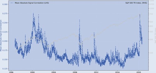
Yet, when we focus on the dynamic behavior of the correlations, figure 1 illustratively shows that correlations become more pronounced (the mean of the absolute correlations increases) during episodes of stock market volatility. For instance, as during the SARS-CoV-2 crisis, the 2008 financial crisis and the Dot-com bubble. In light of our Monte-Carlo simulations, this second piece of evidence indicates that, in the short-run, behavioral biases may become more visible during crises.²

Figure 1. The S&P 500 index and the mean absolute signal correlations.

Notes: sample period: 1996.06–2020.08; The figure shows the relation between the S&P 500 Index and the mean absolute signal correlations between a collection of market-based and fundamental indicators. ${\rho }_{XX}$ is a correlation matrix that contains the cross-correlations between the signals. The mean of the absolute cross-correlations of the signals (the absolute of the elements of ${\rho }_{XX}$) indicates the strength of the correlations. See Section 3.2 for more detail about the signals (predictors).

What are the limitations of our findings? Our interpretations rest on a number of additional assumptions. First, the set of predictors—although containing many of the standard predictors that the literature employs—does not contain all possible predictors. Could the absence of predictors overturn our conclusions? We think this is unlikely for two reasons: (i) since we already use many of the more correlated predictors, the missing predictors are presumably less correlated with subsequent returns and (ii) finding a high joint correlation across signals is more difficult with a larger basket of weakly correlated predictors.

Second, each of our predictors represents a signal that triggers buying and selling by different types of biased, signal-following traders.³ By assuming that predictors act as signals which proxy biases, we also make implicit assumptions about the proportions of trades which are triggered by these signals. For example, claiming that a large basket of uncorrelated signals cancels out in the aggregate, rests on the assumption that trades that follow individual signals face a significant number of opposing trades. While we cannot directly provide evidence for this assumption, we think it is reasonable to assume, given the large number of uncorrelated signals and market participants, that no individual signal generates enough trading volume to counter the trading volume generated by other signals.

Our paper primarily relates to the literature on mispricing due to behavioral biases in financial markets. Numerous papers document various individual behavioral biases see, among many others, e.g. Bondt and Thaler (1985), Lakonishok et al. (1994), Coval and Shumway (2005), DellaVigna and Pollet (2009), Mclean and Pontiff (2016), and Chen and Sabherwal (2019) for potential factors in explaining certain price anomalies. Yet, such papers pay little attention to how individual biases interact and create patterns at the aggregate level. Papers that study the interactions of heterogenous traders remain largely theoretical; see, among many others, e.g. Black (1986), Shleifer and Summers (1990), Brock and Hommes (1997), Shleifer and Vishny (1997), Lux and Marchesi (1999), Sandroni (2000), Boswijk et al. (2007), Yan (2010), Xiong and Yan (2010), Eyster et al. (2019), Peress and Schmidt (2020), and Westphal and Sornette(2020).

We contribute to this literature predominantly by empirically studying the effects of signal interactions on overall return predictability. We highlight the two aforementioned findings. Our methodology benefits from recent computational advances in machine learning, which allow us to study the interactions between predictors see, e.g. Moritz and Zimmermann (2016), Gu et al. (2020), and Kozak et al. (2020) among others. These studies are in contrast to older linear studies such as Fama and French (1992, 2016) that assume no interactions within the set of predictors, and which may consequently hinder predictability. In contrast to the machine learning papers, which focus on demonstrating that interactions and non-linearities may play an important role in explaining the data, we focus on how the interactions across predictors can help us understand why biased traders may not produce more pronounced patterns in the data.⁴

Our findings are further related to studies on herding behavior by investors. As in the literature on ‘style-investing’ (Barberis and Shleifer 2003, Teo and Woo 2004, Boyer 2011), the chosen predictors can be viewed as representative of various styles used by the industry. Thus, our trading signals can proxy for heterogeneous traders that trade on different subsets of such signals. Our empirical findings complement earlier theoretical work on herding by, among many others, Froot et al. (1992), Banerjee (1992), Avery and Zemsky (1998), Dennis and Strickland (2002), Alfarano et al. (2005), Veldkamp (2006), Choi and Sias (2009), Park and Sabourian (2011), Kukacka and Barunik (2013), and Aghamolla and Hashimoto (2020). Like many of these theoretical papers on herding, most empirical studies in this area focus on increasing numbers of traders following the same signals (see, among many others, Grinblatt et al. (1995), Nofsinger and Sias (2002), Peter Chung and Thomas Kim (2017), and Campajola et al. (2020)). By contrast, in our study, herding-like effects do not arise as a result of copy-trading. Rather, we conjecture that, if the correlations between different signals become stronger, herding-like effects may arise and eventually increase market volatility.

Our paper proceeds as follows. Section 2 briefly explains the empirical approach. Section 3 describes the data and the main empirical findings. Section 4 provides a discussion and a theoretical rationale of the empirical evidence. Section 5 concludes. Appendices 1–5 present a variety of robustness tests.

2. Methodology and implementation

At time t, let us define the expected t + 1 response of stock i, $E_t\left(y_{i,t+1}\right)$, as a function g, of a matrix of predictors ${\mathbf{X}}_{i,t}=(x_{i,t,1},x_{i,t,2},\dots ,x_{i,t,N})$. Formally, (1) $E_t\left(y_{i,t+1}\right)=g(x_{i,t,1},x_{i,t,2},\dots ,x_{i,t,N})=g\left({\mathbf{X}}_{i,t}\right).$(1) As financial returns are noisy, we transform the prediction problem into a classification problem. The procedure is called discretization and lowers the impact of extreme returns, thereby reducing the noise (see e.g. Fayyad and Irani (1993) and Garcia et al. (2013)). We categorize the future realized return of asset i, $r_{i,t+1}$, into either one or zero—depending on whether it is positive or negative. More formally, the response variable, $y_{i,t+1}$, is coded as (2) $y_{i,t+1}=\left\{\begin{array}{ll}1,& \mathrm{i}\mathrm{f}{r}_{i,t+1}>0.\\ 0,& \mathrm{o}\mathrm{t}\mathrm{h}\mathrm{e}\mathrm{r}\mathrm{w}\mathrm{i}\mathrm{s}\mathrm{e}.\end{array}\right.$(2) We use two main approaches to approximate g—Logit and Boosted Trees. Our strategy is to predict class probabilities and then evaluate how well these probabilities predict subsequently realized returns. Our main goal is to approximate an upper bound of predictability. Appendices present a large variety of further exercises that support the main findings from Section 3.

3. Empirical analysis

3.1. Data

We focus on stocks in the Russell 1000 universe using end-of-day daily data during 1995.12–2020.08. All data are drawn from Bloomberg.⁵

To address issues arising from survivorship bias, we make two choices. First, we only include observations from those stocks that are members of the Russell 1000 at a given point in time. For example, on 2020.01.30, our sample includes only those stocks that are members of the Russell 1000 on the day of the last rebalancing. Since stocks enter and exit the index over time, our total sample includes about 3000 stocks. Second, we construct an equally weighted long-only benchmark from the exact same pool of stocks as our machine learning strategies. This benchmark is also rebalanced at the same frequency as our machine learning strategies.

For the forecasting and rebalancing horizon, we choose periods no greater than one month, as longer horizons are notoriously difficult to predict. Trading costs are negligible and affect all strategies and benchmarks symmetrically in our analysis.

Stock prices and volumes are adjusted for spin-offs, stock splits, consolidations, rights offerings, entitlements, stock dividends and bonuses. Historical pricing reflects normal cash dividends including regular cash, interim, income, estimated, partnership distribution, final, prorated, interest on capital, and distribution type dividends. It also reflects abnormal cash dividends including special cash, liquidating, capital gains (both long- and short-term), memorial, return of capital, rights redemption, proceeds/rights, proceeds/shares, proceeds/warrants, and miscellaneous return premia.

We focus on a set of 50 predictors that are available for all stocks. Despite extensive data availability, there are NaN gaps in the data. It is important to mention that the Logit approach cannot deal with NaNs and thus obtains the parameters from a reduced in-sample period. In contrast, Boosting can account for NaNs and estimates from a larger in-sample period. Appendix 4 reports the boosting results from an in-sample period containing only non-NaN observations.

Our sample is split into an in-sample (1995.12–2013.12) and an out-of-sample period (2013.12–2020.08). Since we focus on biases, we choose a rather late cut-off, as patterns and biases are usually arbitraged away when the market learns of them, e.g. Kolev and Karapandza (2017). In Appendix 2, we present results for a different cut-off.

Data scaling is a recommended pre-processing step when working with noisy data. To normalize the predictors, we employ a simple ranking and then scale it between zero and unity. This procedure is equivalent to imposing the empirical cumulative distribution function on the data and converting the actual values to their corresponding probabilities. The advantage of this method is that it linearizes the predictors and thus mitigates the impact of outliers. Formally, (3) $x_{i,t,n}^{\prime }=\frac{1}{M}\sum _{t=1:T}\sum _{i=1:I}{\mathbb{1}}_{x_{i,t,n}<z},$(3) where ${\mathbb{1}}_{x_{i,t,n}<z}$ is an indicator variable denoting the elements smaller than z and $M=I\ast T$ the total number of elements. Appendix 5 provides a robustness test where we use the empirical cumulative distribution instead.

More importantly, we use commonly accepted predictors that have been documented in previous studies. Our interpretation is that these signals have predictive power as they represent either biases or risks. The true source of the predictability is not important since our goal is to measure an upper bound on return predictability. Our main claim is that trader biases cannot account for more than this upper bound. Thus, even if some of the predictors reflect a risk, our central claim is still valid.

3.2. Signals

While smaller than (Gu et al. 2020), our set of predictors is sufficient to achieve a similar out-of-sample explanatory power as we will see further below. The predictors we use are motivated by previous studies—although each is specifically calculated, they should be correlated with broad categories of factors that have been shown to explain return variability. These classes include size, value, momentum, crash-risk, and liquidity; see, e.g. Sharpe (1964), Fama and French (1992), Longstaff (1995), Asness et al. (2013), Novy-Marx and Velikov (2015), Farhi and Gabaix (2016), Harvey et al. (2016), Struck and Cheng (2019), Freyberger et al. (2020), among others.

Momentum. We use four different measures of Time Series Momentum with different lags of 10, 20, 60, 180 business days. This is calculated as: $x_{i,t,1-4}=\frac{P_{i,t}}{P_{i,t-q}}-1\mathrm{\forall }q\in \{10,20,60,180\}$ where q denotes the number of workdays and determines the length of the look-back window; $P_{i,t}$ is the level of the excess return series of commodity i at time t.

Volatility. Our second set of predictors measure past daily volatility and is thus similar to the risk measure hypothesized by Sharpe (1964). Formally, $\begin{array}{rl}& x_{i,t,5-8}=\sqrt{\frac{1}{Q-1}\sum _{q=0:Q}(P_{i,t-q}-{\mu }_Q{)}^2}\\ & \mathrm{\forall }Q\in \{10,20,60,180\}\end{array}$ where the look-back window Q, is given by the number of weekdays, and ${\mu }_Q$ denotes the average price over that window. By using the levels instead of the changes, we give this measure a little twist drawing on an insight in a recent paper by Shue and Townsend (2020) that emphasizes that price levels may contain valuable information to predict returns. We also consider at-the-money implied volatility of the first listed expiry at least 20 business days from today: $x_{i,t,9}={\text{iVol}}_{100,i,t}^{30\mathrm{d}\mathrm{a}\mathrm{y}\mathrm{s}}$ Implied out-of-the-money volatility can also be used to construct a measure of risk reversal. We use the difference between the implied 30-day volatility of the out-of-the-money 95% put and 105% call options. Intuitively, this difference in option implied volatility indicates expectations of market participants in whether the 1-month return risk is skewed above or below the at-the-money strike. Our measure is calculated as: $x_{i,t,10}={\text{iVol}}_{95,i,t}^{30\mathrm{d}\mathrm{a}\mathrm{y}\mathrm{s}}-{\text{iVol}}_{105,i,t}^{30\mathrm{d}\mathrm{a}\mathrm{y}\mathrm{s}}$ Finally, we also consider the short term momentum, or change, in implied volatility: $x_{i,t,11-12}=\frac{{\text{iVol}}_{100,i,t}}{{\text{iVol}}_{100,i,t-q}}-1\mathrm{\forall }q\in \{10,20\}$ Correlation. Our third set of predictors measures the past daily correlation of each stock with the market. The market correlation is approximated here by the median stock correlation in the sample. We denote that as: $x_{i,t,13-14}=\mathbf{C}\mathbf{o}\mathbf{r}\mathbf{r}(P_{i,t:t-Q},P_{\mathrm{\neg }i,t:t-Q})\mathrm{\forall }Q\in \{20,60\}$ and the look-back window Q, is given by the number of weekdays. Again, relying on the same argument as before, we use the level instead of the change.

Skewness and Kurtosis. We also use the empirical skewness and the kurtosis of the daily returns over the past year. Skewness give us actual realized directional market risks, as compared to the option implied risk-reversal, which measures expected directional risks. Skewness and kurtosis are respectively defined as: $\begin{array}{rl}& x_{i,t,15}=\frac{\frac{1}{Q}{\displaystyle \sum _{q=0:Q}{\left(P_{i,t-q}-{\mu }_Q\right)}^3}}{{\left(\sqrt{\frac{1}{Q}{\displaystyle \sum _{q=0:Q}{\left(P_{i,t-q}-{\mu }_Q\right)}^2}}\right)}^3}\\ & x_{i,t,16}=\frac{\frac{1}{Q}{\displaystyle \sum _{q=0:Q}{\left(P_{i,t-q}-{\mu }_Q\right)}^4}}{{\left(\sqrt{\frac{1}{Q}{\displaystyle \sum _{q=0:Q}{\left(P_{i,t-q}-{\mu }_Q\right)}^2}}\right)}^4}\end{array}$ where Q is set to be 260 weekdays. Again, relying on recent findings by Shue and Townsend (2020), we use the level instead of the change.

Size. We compute a measure of size by measuring a moving average of the daily turnover times the share price: $x_{i,t,17}=\frac{\frac{1}{Q}{\displaystyle \sum _{q=0:Q}{\mathrm{t}\mathrm{u}\mathrm{r}\mathrm{n}}_{i,t-q}}}{\frac{1}{Q}\frac{1}{j}{\displaystyle \sum _{q=0:Q}\sum _j{\mathrm{t}\mathrm{u}\mathrm{r}\mathrm{n}}_{j,t-q}}}$ where ${\mathrm{t}\mathrm{u}\mathrm{r}\mathrm{n}}_{i,t}$ is the trading turnover (in USD) of stock i at time t relative to all other stocks j in the Russell 1000. We set Q to be 60 business days.

Value. We use several ratios from the cash-flow statement. Our measures of firm value include the Price Earnings ratio of the firm and the firm's Price Earnings ratio relative to that of the Russell 1000 index: $\begin{array}{rl}& x_{i,t,18}=P_{i,t}/E_{i,t}\\ & x_{i,t,19}=\left(P_{i,t}/E_{i,t}\right)\left(P_{\text{Russell 1000},t}/E_{\text{Russell 1000},t}\right)\end{array}$ where $E_{i,t}$ is the trailing 12M earnings per share before extraordinary items. We also include the Price to Sales ratio and the Price to Cash-flow per share ratio: $\begin{array}{rl}& x_{i,t,20}=\left(P_{i,t:t-5\ast 260}/S_{i,t:t-5\ast 260}\right)-\left(P_{i,t}/S_{i,t}\right)\\ & x_{i,t,21}=\left({\text{P}}_{i,t}\right)/{\text{CF}}_{i,t}\end{array}$ where $S_{i,t}$ denotes Sales per share and is calculated on a trailing 12 month basis by adding the most recent four quarters. ${\text{CF}}_{i,t}$ denotes the cash-flow per share.

From the balance sheet, we use the Price to Book ratio and the Enterprise Value to Book value ratio. The first ratio captures the public market implied growth prospects of the firm, while the second is a measure of how much an acquirer would value the firm: $\begin{array}{rl}{x}_{i,t,22}& =P_{i,t}/B{V}_{i,t}\\ x_{i,t,23}& =\left({\text{EV}}_{i,t}\right)/{\text{BV}}_{i,t}.\end{array}$ Liquidity. We include several measures of leverage and liquidity. The Current ratio indicates a company's ability to fulfill its short-term liabilities using short-term assets, and the Cash ratio measures immediate liquidity needs. They are respectively defined as: $\begin{array}{rl}& x_{i,t,24}=A_{i,t}/L_{i,t}\\ & x_{i,t,25}=({\text{Cash}}_{i,t}+{\text{Near Cash Items}}_{i,t}\\ & +{\text{Marketable Securities}}_{i,t})/{\text{Current Liabilities}}_{i,t}\end{array}$ where $A_{i,t}$ and $L_{i,t}$ denotes the short term assets and liabilities. Closely related to these ratios is the Interest Coverage ratio, which is used to measure the burden of debt interest payments out of annual operating income (also known as earnings before interest and taxes, or EBIT): $\begin{array}{rl}& x_{i,t,26}=\left({\text{Earnings before Interest and Taxes}}_{i,t}\right)\\ & /{\text{Total Interest Incurred}}_{i,t}\end{array}$ Leverage. If firms cannot meet their liabilities, equity serves as a buffer before liquidation. We consider two measures of leverage: the Tangible Common Equity to Asset ratio, and a liquidation ratio. Using tangible values may be more realistic during a distressed liquidation. In this calculation, both the total assets and the common equity are adjusted downward by the amount of intangible assets (including goodwill, licenses, trademarks, copyrights, etc.). $x_{i,t,27}=100\ast {\text{Tangible Common Equity}}_{i,t}/{\text{Tangible Assets}}_{i,t}$ We also include a liquidation ratio which measures a company's ability to cover debt obligations with its assets, after all short-term liabilities have been satisfied: $\begin{array}{rl}{x}_{i,t,28}& =\left[\right({\text{Book Value of Total Assets}}_{i,t}\\ & -{\text{Total Intangible Assets}}_{i,t})-({\text{Current Liabilities}}_{i,t}\\ & -{\text{Short Term Borrowings}}_{i,t}\left)\right])\\ & /{\text{Total Debt Outstanding}}_{i,t}.\end{array}$ Investment and ROIC. To capture predictors of future firm growth and its investment efficiency, we examine two ratios. First, the Operating Cash to Capex ratio, which indicates how much of operating cash is used to service Capex. The intuition here is that growing firms tend to invest more. This measure is also industry specific. For example, for industrials and banks, it is given as $x_{i,t,29}=\left(\text{Cash from Operations}{)}_{i,t}/\right(\text{Capital Expenditures}{)}_{i,t}$ In addition to the dollar value of investment, we are interested in its efficiency. The Return on Invested Capital (ROIC) divided by Weighted Average Cost of Capital (WACC) ratio indicates how efficiently firms are using their investment funds: $x_{i,t,30}=\left({\text{ROC}}_{i,t}\right)/{\text{WACC}}_{i,t}$ Industry Specific Effects. We employ a set of industry dummies to control for differences across industries. More specifically, we use the Industry Classification Benchmark (ICB) super-sector classification which divides companies into 19 super sectors: Automobiles & Parts (3300), Banks (8300), Basic Resources (1700), Chemicals (1300), Construction & Materials (2300), Financial Services (8700), Food & Beverage (3500), Health Care (4500), Industrial Goods & Services (2700), Insurance (8500), Media (5500), Oil & Gas (0500), Personal & Household Goods (3700), Real Estate (8600), Retail (5300), Technology (9500), Telecommunications (6500), Travel & Leisure (5700), Utilities (7500).

3.3. Main findings

Our main results are summarized in table 1. The table shows the mean, median, max, min, and standard deviation of the correlations between the model predicted probabilities and the realized returns for different samples. It includes (i) an all stocks sample and (ii) samples at the extremes (sorted by predicted probabilities). There are three main takeaways. First, Boosted Trees slightly outperforms the Logistic approach in terms of out-of-sample predictability at the extremes as measured by a higher mean correlation between predicted and realized returns. As the Appendices show, this result passes a number of robustness tests. For instance, in the all top/bottom 10 stocks sample, the mean Pearson correlation is 0.08 for Boosted Trees and 0.06 for the Logistic approach. Second, out-of-sample predictability for both the Logistic approach and Boosted Trees increases at the extremes. For example, under Boosted Trees, the Pearson out-of-sample correlation in the group of the top and bottom 10 stocks is 0.08 while it is only 0.02 in the all stocks sample. Third, the highest out-of-sample $R^2$ (the squared correlation) is less than 1% (Boosted Trees, Top/Bottom 10, Pearson: 0.08). This finding is quantitatively in line with the findings of Gu et al. (2020) using a different sample of U.S. stocks and also a different sample period. In contrast to their results, the linear approach does not lag far behind the tree-based approach in our analysis. This may potentially be due to the fact that our predictor normalization procedure effectively linearizes the data. Appendix 5 shows that the Logistic Classification predictability decreases under an alternative normalization procedure that does not linearize the data.

Table 1. Predicted vs. realized returns (main result, out-of-sample).

Method	Measure	Entire sample	Top/Bottom 50	Top/Bottom 20	Top/Bottom 10
Logistic classification	Mean	0.03	0.05	0.06	0.06
	Median	0.03	0.05	0.06	0.08
	Max	0.28	0.58	0.77	0.81
	Min	−0.27	−0.55	−0.68	−0.75
	Std	0.09	0.17	0.23	0.29
Boosted trees	Mean	0.02	0.06	0.07	0.08
	Median	0.02	0.06	0.07	0.08
	Max	0.45	0.67	0.78	0.91
	Min	−0.44	−0.66	−0.76	−0.84
	Std	0.1	0.2	0.26	0.31

Notes: bi-weekly forecast horizon and rebalancing; in-sample period: 1995.12–2013.12; out-of-sample period: 2013.12–2020.08; Stock Sample: Russell 1000. This table shows the pooled correlations (across stocks and points in time) between predicted and subsequently realized returns.

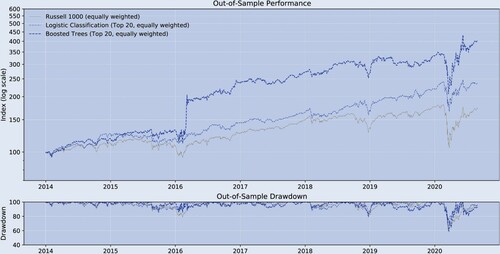
To confirm that the previously shown relatively low out-of-sample predictability contains some information (and is not just noise), table 2 and figure 2 translate the return predictability into long-only trading strategies. All trading strategies are rebalanced bi-weekly at end-of-day prices. The benchmark is the equally weighted long-only Russell 1000. A marketcap-weighted index would have performed similarly. From the Logistic approach and Boosted Trees we form a trading strategy where we sort the universe biweekly by probability, and then take the top 20 of these rankings to form an equally weighted portfolio. The figure shows that the two strategies outperform out-of-sample in terms of absolute returns while exhibiting a drawdown profile similar to the benchmark.

Figure 2. Historical performance (main result, out-of-sample).

Notes: bi-weekly forecast horizon and rebalancing; in-sample period: 1995.12–2013.12; out-of-sample period: 2013.12–2020.08; Stock Sample: Russell 1000. This figure compares the performance of the different trading strategies.

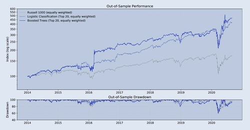
Table 2. Performance indicators (main result, out-of-sample).

	Indicator	2014	2015	2016	2017	2018	2019	2020	Overall
Russell 1000 (eq w)	Return(%)	11.42	−3.15	16.32	18.66	−8.96	29.92	−2.0	8.54
	Volatility (%)	12.41	15.48	16.53	8.14	16.09	13.56	47.27	19.97
	max Drawdown	−9.53	−13.62	−12.64	−3.67	−21.54	−7.49	−41.67	−41.67
	Sharpe Ratio	0.92	−0.2	0.99	2.29	−0.56	2.21	−0.04	0.43
	Return to $|$max Drawdown$|$	1.2	−0.23	1.29	5.09	−0.42	4.0	−0.05	0.2
	Market Correlation	1.0	1.0	1.0	1.0	1.0	1.0	1.0	1.0
Logistic (Top 20, eq w)	Return(%)	16.99	16.65	28.55	23.5	14.97	35.65	22.62	23.78
	Volatility(%)	11.43	15.12	19.12	8.91	15.05	12.36	48.88	20.37
	max Drawdown	−7.41	−10.25	−10.34	−4.36	−12.4	−7.12	−39.17	−39.17
	Sharpe Ratio	1.49	1.1	1.49	2.64	0.99	2.88	0.46	1.17
	Return to $|$max Drawdown$|$	2.29	1.62	2.76	5.39	1.21	5.01	0.58	0.61
	Market Correlation	0.86	0.89	0.81	0.78	0.88	0.81	0.89	0.85
Boosted T (Top 20, eq w)	Return(%)	17.2	11.51	75.88	16.88	−2.24	29.37	38.83	26.22
	Volatility (%)	11.4	14.53	36.33	10.93	16.12	17.2	57.7	26.13
	max Drawdown	−7.98	−12.32	−13.57	−7.49	−20.34	−13.34	−40.42	−40.42
	Sharpe Ratio	1.51	0.79	2.09	1.55	−0.14	1.71	0.67	1.0
	Return to $|$max Drawdown$|$	2.15	0.93	5.59	2.26	−0.11	2.2	0.96	0.65
	Market Correlation	0.88	0.87	0.86	0.72	0.86	0.88	0.87	0.85

Notes: bi-weekly forecast horizon and rebalancing; in-sample period: 1995.12–2013.12; out-of-sample period: 2013.12–2020.08; Stock Sample: Russell 1000. This table shows a variety of performance measures for different trading strategies.

Table 2 confirms this impression. It presents a variety of performance measures. Over the out-of-sample period 2013.12–2020.8, both the Logistic approach and Boosted Trees outperform the long-only Russell 1000. During this period, both strategies feature better drawdown behavior, with the maximum drawdowns being $-41.67\mathrm{\%}$ for the Russell 1000, $-39.17\mathrm{\%}$ for the Logistic approach and $-40.42\mathrm{\%}$ for Boosted Trees. The smaller drawdowns and higher returns are reflected in better overall annual risk-adjusted measures, including the return-to-absolute max drawdown ratio and the Sharpe ratio. Our results indicate that the low predictability of $1\mathrm{\%}$ contains valuable information leading to outperformance. This is consistent with (Moritz and Zimmermann 2016) whom, using a different stock sample and sample period, find significant improvement in terms of risk-adjusted returns, by employing big-data and non-linear methods over a passive investment approach.

4. Interpretation

Even when we employ advanced regression techniques such as Boosted Trees, we are only able to predict a small fraction of return variation out-of-sample. We now turn to addressing our second main question—given the weak evidence we find for systematic patterns, why do these biases not show up more clearly in the markets? We focus on a possible explanation that we derive from De Long et al. (1990), and Fama (1965): the presence of many uncorrelated signals may lead to biases canceling out at the aggregate level.

The predictability, $R^2$, can be determined from the cross-correlations. We consider a multiple linear regression problem with N explanatory variables and split their linear correlations into two groups: (i) the predictor-return correlations, ${\rho }_{n,t}=\mathbf{C}\mathbf{o}\mathbf{r}\mathbf{r}(r_{t+1},x_{n,t})$ and ii) the predictor correlations, ${\rho }_{n,m,t}=\mathbf{C}\mathbf{o}\mathbf{r}\mathbf{r}(x_{n,t},x_{m,t})$ where $n,m\in \{1,2,\dots ,N\}$. Define in vector/matrix form these two respectively by: $\begin{array}{rl}{\rho }_{r_{t+1},{\mathbf{X}}_{\mathbf{t}}}& =\left|\begin{array}{c}{\rho }_{1,t}\\ {\rho }_{2,t}\\ ⋮\\ {\rho }_{N,t}\end{array}\right|,\\ {\rho }_{{\mathbf{X}}_{\mathbf{t}}{\mathbf{X}}_{\mathbf{t}}}& =\left|\begin{array}{cccc}{\rho }_{1,1,t}& {\rho }_{1,2,t}& \dots & {\rho }_{1,N,t}\\ {\rho }_{2,1,t}& {\rho }_{2,2,t}& \dots & {\rho }_{2,N,t}\\ ⋮& ⋮& \ddots & ⋮\\ {\rho }_{N,1,t}& {\rho }_{N,2,t}& \dots & {\rho }_{N,N,t}\end{array}\right|.\end{array}$ The vector contains the correlations between the returns and each of the predictor variables. The matrix contains the correlations between each pair of predictor variables. The $R_t^2$ of the multiple linear regression problem is given by: $R^2={\rho }_{r,X}^T{\rho }_{X,X}^{-1}{\rho }_{r,X}$. (We omit the time subscripts to improve readability).

In our context, we split the analysis into two parts. First, we examine the empirical predictor correlation matrix, ${\rho }_{\mathbf{X}\mathbf{X}}$. Second, we focus on the predictor-return correlations vector, ${\rho }_{r,\mathbf{X}}$. Besides investigating the empirical correlation matrix, we conduct Monte-Carlo simulations to generate random correlation matrices under certain distributional assumptions. These simulations serve as a counterfactual from which we can draw conclusions.

For the simulations, we begin by generating strictly positive random eigenvalues from a uniform distribution. To ensure that the sum of the eigenvalues is equal to the number of predictors, we pre-multiply all eigenvalues with a common factor. We then use a numerically fast procedure by Davies and Higham (2000), based on the popular algorithm of Bendel and Mickey (1978), which takes a matrix having the specified eigenvalues and uses a sequence of Givens rotations to introduce ones on the diagonal.

Figure 3 plots the results. Panel A shows the distributions of the elements of ${\rho }_{XX}$ estimated from the out-of-sample period 2013.12–2020.08. The correlations are mainly distributed around zero with a much high kurtosis than a normal distribution. Are those weak correlations responsible for the low $R^2$? Panel B shows the $R^2$'s calculated from 1000 simulated matrices. In the simulations, the correlation distribution is assumed to be normal with mean zero, which leads to a higher $R^2$ by assumption. Yet, despite the normality assumption, the panel clearly shows that most of the generated $R^2$s are close to zero. Panels C and D then plot the distributions of the correlations in the case of the (i) lowest generated $R^2$ and (ii) highest generated $R^2$.

Figure 3. Monte-Carlo correlations: varying ${\rho }_{XX}$, normal distribution.

Notes: bi-weekly forecast horizon and rebalancing; in-sample period: 1995.12–2013.12; out-of-sample period: 2013.12–2020.08; Stock Sample: Russell 1000. Panel A shows the distribution of the empirical predictor correlations ${\rho }_{XX}$. Panel B shows the distribution of the simulated $R^2$'s. Panel C shows the distribution of the simulated predictor correlations ${\rho }_{XX}$ that yielded the lowest $R^2$. Panel D shows the distribution of the simulated predictor correlations ${\rho }_{XX}$ that yielded the highest $R^2$.

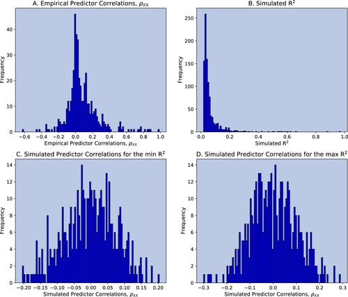
Figure 4 then illustrates that a higher $R^2$ can be generated easily with a distribution of correlations that is very different from the one that is empirically observed.⁶ When the predictor correlations are closer to $+1$ and $-1$, we are much more likely to find high predictability. This second figure serves as our counterfactual. Combining the information from the two figures, we argue that the empirically weak correlations within the set of predictors support our hypothesis that uncorrelated signals result in a low general predictability of stock returns in the long-run. Intuitively, a noise trader who may respond to a 2-weeks Momentum signal—one of the predictors in our data—may buy a stock matching with another noise trader who may respond to a selling signal thus muting the overall impact of the first signal.

Figure 4. Monte-Carlo correlations: varying ${\rho }_{XX}$, bimodal distribution.

Notes: bi-weekly forecast horizon and rebalancing; in-sample period: 1995.12–2013.12; out-of-sample period: 2013.12–2020.08; Stock Sample: Russell 1000. Panel A shows the distribution of the empirical predictor correlations ${\rho }_{XX}$. Panel B shows the distribution of the simulated $R^2$'s. Panel C shows the distribution of the simulated predictor correlations ${\rho }_{XX}$ that yielded the lowest $R^2$. Panel D shows the distribution of the simulated predictor correlations ${\rho }_{XX}$ that yielded the highest $R^2$.

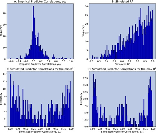
Table 3 (as well as figure 1 in the introduction) then focuses on the time series dynamics of the empirical signal correlation matrix, ${\rho }_{XX}$. The matrix is constructed on a daily basis. To capture both short-term time-series and cross-sectional variation, we use three alternative matrixes. The first contains only the cross section, i.e. trading day t as indicated in the table as Pred Corr (t). The second contains trading day t and the trading day 20 days before as indicated in the table as Pred Corr (t, t-20). The third contains trading day t and the trading day 60 days before as indicated in the table as Pred Corr (t, t-60). It shows that there is a strong positive relation between the market implied volatility and the strength of the correlations between signals (in ${\rho }_{XX}$).

Table 3. Implied market volatility and signal correlations (${\rho }_{XX}$).

Predictor Correlation	Subsample	abs(${\rho }_{XX}$)	CBOE VIX	Median iVol	Mean iVol
Pred Corr (t)	1996.06–2020.08	Median	0.35	0.41	0.43
		Mean	0.39	0.46	0.49
	2013.12–2020.08	Median	0.23	0.28	0.25
		Mean	0.32	0.37	0.34
Pred Corr (t,t-20)	1996.06–2020.08	Median	0.37	0.43	0.45
		Mean	0.45	0.52	0.54
	2013.12–2020.08	Median	0.26	0.35	0.32
		Mean	0.39	0.46	0.43
Pred Corr (t,t-60)	1996.06–2020.08	Median	0.39	0.43	0.45
		Mean	0.5	0.55	0.57
	2013.12–2020.08	Median	0.31	0.29	0.26
		Mean	0.39	0.39	0.36

Notes: Sample period: 1996.06–2020.08; The figure shows the relation between implied market volatility as measured by (i) the CBOE Volatility Index (VIX), (ii) the median and (iii) the mean implied 30-days at the money volatility of stocks in the Russell 1000; the strength of the correlations across signals as measured by (a) the median and (b) the mean absolute correlation in the Signal Correlations Matrix, ${\rho }_{XX}$. There are three samples for the predictor correlations: (i) day t, (ii) day t and day t-20, and (iii) day t and day t-60.

Figure 1 in the introduction confirms this impression. It shows that signal correlations becoming more pronounced (the sum of the absolute correlations increases) coincides with episodes of stock market volatility during the SARS-CoV-2 crisis, the 2008 financial crisis, and the Dot-com bubble. In the light of our Monte-Carlo simulations, this second piece of evidence supports the hypothesis that, in the short-run, when noise traders become more correlated, their aggregate behavior may eventually increase volatility (see, e.g. Dennis and Strickland (2002), and Choi and Sias (2009)).

Based on the evidence we obtained from our Monte-Carlo Simulations, we do not expect signal correlations to explain a major part of market volatility. First, there are still many other drivers of volatility such as news. Second, even when the correlations among signals become stronger, this only raises the probability of having noise traders act together in the aggregate. Their actions may still cancel out (thus not raising volatility), even as their signals are more strongly correlated. Third, figure 1 shows that signal correlations never become very strong, with the sum of absolute predictor correlation not increasing by more than 100% during peak times. By contrast, figure 4 emphasizes that signal correlations must be close to $+1$ and $-1$ for a sufficiently high probability of signals to not cancel out.

Our interpretation rests on two additional assumptions. First, the set of predictors—although containing many of the main standard predictors that the literature describes—does not contain all possible predictors. However, we do not think that the presence of other predictors would overturn our conclusions. Given the many predictors that have been studied, and the determination that very few of them are significant, any other predictors would be even more weakly correlated with returns than the ones we use. A larger set of predictors would also result in less correlated actions by signal-following noise traders. As the number of weakly correlated signals grows, it becomes more likely that they cancel out.

Second, each of our predictors represents a signal that triggers buying and selling by different types of biased, signal-following traders. By assuming that predictors reflect signals and biases, we also make implicit assumptions about the proportions of trades which are triggered by these signals. For example, claiming that a large basket of uncorrelated signals cancels out at the aggregate, rests on the assumption that trades triggered by individual signals face a significant number of opposing trades. However, given the large number of uncorrelated signals and market participants, we think it is reasonable to assume that no individual signal generates enough trading volume to overcome trading volume generated by other signals.

5. Conclusions

Behavioral economics makes numerous empirical observations in financial markets that may result from biased, signal-following traders. To what degree do these biases create systematic patterns in the markets? Analyzing U.S. equities, we find that the evidence for systematic patterns is rather small.

More specifically, using over 50 popular predictors (signals) to forecast the cross-section of stock returns in the Russell 1000 over a horizon of 1 month or less, we find that return predictability is less than 1%. This latter piece of evidence warrants explanation given the large number of well-documented behavioral biases.

Our explanation makes an analogy by borrowing the term antinoise from the audio signal processing literature. Studying the empirical correlation structure of our signals, we find that, over the long-run, the correlations are mainly distributed around zero with a much higher kurtosis than a normal distribution. Employing Monte-Carlo methods, we verify that to find predictability of more than $1\mathrm{\%}$ is an unlikely outcome given such a correlation structure. By contrast, we show that under a bimodal distribution with many correlations close to −1 and +1, finding high predictability is a more likely outcome.

Applying our antinoise analogy to financial markets is straightforward: a trader responding to a two-weeks Momentum signal—one of the predictors in our data—may want to buy a stock matching with another trader responding to a sell signal thus muting the overall impact of the first signal. With many uncorrelated signals in place, there is a high probability that each signal will face an opposing signal at each point in time. As a result of the presence of antinoise, we do not expect to find high return predictability.

However, focusing on the dynamic behavior of the correlations, we find that correlations become more pronounced during episodes of stock market volatility. For instance, during the SARS-CoV-2 crisis, the 2008 financial crisis, and the Dot-com bubble. In light of our Monte-Carlo simulations, this second piece of evidence indicates that in the short-run behavioral biases may become more visible during crises.

Acknowledgments

We thank Frank Fabozzi, David-Michael Lincke, Stefan Nagel, Andrei Shleifer, Friedrich Wetterling, Karl Whelan as well as the editor, Jim Gatheral, and two anonymous referees for meaningful feedback that helped us improve our work. Annika Sophia Benecke and Ancil Crayton provided outstanding research assistance.

Disclosure statement

No potential conflict of interest was reported by the author(s).

Notes

1 In the Appendices, we show how this finding is robust to (A) varying the number of long-positions in the portfolio (B) using an alternative in-sample/out-of-sample split (C) rebalancing and forecasting at a weekly or monthly frequency (D) using different sets of boosting parameters (E) employing an alternative predictor normalization procedure.

2 The reason is that the chance of actions canceling out amid strong correlations between signals is lower. Intuitively, with strong correlations between signals, we would need the negative and positive signals to trigger quantitatively identical opposing bets in order for trades to cancel out in the aggregate—a highly unlikely scenario, which we verify in our Monte-Carlo simulations.

3 There is a large literature that argues that return predictability is caused by predictors representing risk premia. This interpretation would only strengthen our argument, as it would imply that the predictability we discover is the result of biases. The current scientific limitations in this field do not allow us to distinguish between these two sources of predictability. This is why we abstain further from investigating the deeper roots of predictability.

4 Our emphasis is on robustness in this context, as non-parametric methods such as Boosted Trees suffer from high variability when applied to noisy data, as with the relation between predictors and returns in financial markets. We also studied neural networks, but had difficulties obtaining robust results that could be replicated. The results from these networks vastly changed when using different random number seeds. Even averaging the results from hundreds of randomly drawn seeds did not ensure stability of the results.

5 As tree estimations are highly sensitive in noisy environments, we average the estimated models several hundred times. The computations are therefore quite demanding. Hence, we rely on a computationally efficient Boosting procedure from Microsoft called LightGBM in combination with an Amazon Web Services (AWS) cluster with 10 instances of 96 virtual CPUs with 768GB RAM each. The code is a mixture of C, C++, and Python. This combination allows us to complete the computations within a single day. For Boosting we use a set of standard parameters. The results under alternative boosting parameters are reported in Appendix 4.

6 To generate a correlation matrix with a bimodal distribution, we follow a simple three step procedure: (i) generate a symmetric random matrix $\mathbf{A}$, where each column is drawn from a normal distribution and add a fixed constant premultiplied by a random value from a normal distribution which later governs the shape of the distribution, (ii) $\mathbf{B}=\mathbf{A}{\mathbf{A}}^T$, (iii) $\mathbf{C}={\mathbf{D}}^{-0.5}\mathbf{B}{\mathbf{D}}^{-0.5}$, where $\mathbf{D}=\text{diag}\mathbf{B}$.

Appendices

Appendix 1. Robustness: varying the number of long positions

As the first robustness test, we alter the number of long positions of the strategies. In contrast to the main text, where we choose 20 stocks, here we also test for portfolios consisting of 10, and 50 stocks. Figure A1 shows the performance for the Logistic approach and Boosted Trees, respectively. Both figures reveal that the absolute return is highest when the portfolio with only 10 stocks is chosen, followed by 50 stocks. Table A1 shows the performance in more detail. Surprisingly, it reveals that the risk-adjusted returns of the strategies with only 10 stocks is higher than those with 50 stocks. In this context it is important to emphasize that our out-of-sample period is relatively short and does not contain any periods with more than one tail event. Nonetheless, this outperformance may be attributed to our finding that the regression approaches are better able to predict at the extremes of the stock ranking.

Figure A1. Historical performance (Robustness test A, out-of-sample).

Notes: bi-weekly forecast horizon and rebalancing; in-sample period: 1995.12–2013.12; out-of-sample period: 2013.12–2020.08; Stock Sample: Russell 1000. This figure compares the performance of the different trading strategies.

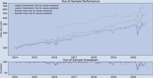
Table B1. Performance indicators (Robustness test A, out-of-sample).

	Indicator	2014	2015	2016	2017	2018	2019	2020	Overall
Logistic (Top 10, eq w)	Return(%)	19.74	17.96	22.33	24.24	23.37	39.64	35.22	27.32
	Volatility(%)	11.4	13.67	20.81	9.37	14.61	11.38	45.74	19.63
	max Drawdown	−6.49	−12.67	−10.63	−4.05	−12.06	−5.08	−34.08	−34.08
	Sharpe Ratio	1.73	1.31	1.07	2.59	1.6	3.48	0.77	1.39
	Return to $|$max Drawdown$|$	3.04	1.42	2.1	5.99	1.94	7.8	1.03	0.8
	Market Correlation	0.8	0.86	0.76	0.7	0.79	0.73	0.83	0.78
Logistic (Top 50, eq w)	Return(%)	18.01	7.74	29.85	18.56	4.34	42.38	5.02	18.24
	Volatility(%)	11.55	15.45	18.04	8.62	15.4	12.57	47.96	20.09
	max Drawdown	−7.62	−10.58	−10.01	−3.95	−16.19	−5.6	−41.6	−41.6
	Sharpe Ratio	1.56	0.5	1.66	2.15	0.28	3.37	0.1	0.91
	Return to $|$max Drawdown$|$	2.36	0.73	2.98	4.69	0.27	7.57	0.12	0.44
	Market Correlation	0.91	0.94	0.88	0.86	0.95	0.9	0.96	0.92
Boosted T (Top 10, eq w)	Return(%)	28.21	18.81	99.26	21.9	7.7	23.39	43.67	34.1
	Volatility(%)	12.32	16.68	45.61	12.2	16.57	19.87	56.94	28.69
	max Drawdown	−5.93	−13.11	−16.95	−7.21	−17.82	−15.15	−35.49	−35.49
	Sharpe Ratio	2.29	1.13	2.18	1.8	0.46	1.18	0.77	1.19
	Return to $|$max Drawdown$|$	4.76	1.43	5.86	3.04	0.43	1.54	1.23	0.96
	Market Correlation	0.8	0.79	0.8	0.61	0.8	0.82	0.85	0.79
Boosted T (Top 50, eq w)	Return(%)	16.66	7.55	57.71	13.81	−8.42	37.07	16.53	19.59
	Volatility(%)	11.0	14.37	28.13	10.04	16.07	15.5	55.2	23.69
	max Drawdown	−7.54	−11.9	−11.56	−6.42	−20.2	−8.58	−40.29	−40.29
	Sharpe Ratio	1.51	0.53	2.05	1.38	−0.52	2.39	0.3	0.83
	Return to $|$max Drawdown$|$	2.21	0.63	4.99	2.15	−0.42	4.32	0.41	0.49
	Market Correlation	0.91	0.93	0.91	0.85	0.93	0.92	0.94	0.91

Notes: bi-weekly forecast horizon and rebalancing; in-sample period: 1995.12–2013.12; out-of-sample period: 2013.12–2020.08; Stock Sample: Russell 1000. This table shows a variety of performance measures for different trading strategies.

Appendix 2. Robustness: alternative in-sample period

As the second robustness test, we choose a different cut-off between the in-sample and the out-of-sample period. For the in-sample period, we choose 1995.12–2016.12 whereas, in the main text, we use 1995.12–2013.12. With bi-weekly rebalancing, we are still left with 88 out-of-sample observations. Table A2 is broadly in line with the corresponding table from the main text. In comparison to the original table, this table shows that (i) Boosted Trees underperforms the Logistic approach in terms of out-of-sample mean correlations, (ii) the mean out-of-sample correlations for both the Logistic approach and Boosted Trees increases at the extremes, and (iii) the highest out-of-sample $R^2$ (the squared correlation) is less than 1% (Logistic Classification, Top/Bottom 10, Pearson: 0.10). Figure A2 and table A3 are also broadly in line with their counterparts in the main text. Namely, the Logistic approach and Boosted Trees outperform the long-only benchmark both in terms of absolute returns over the entire out-of-sample period. In contrast to the main text, Boosted Trees performance lags behind the Logistic approach.

Figure A2. Historical performance (robustness test B, out-of-sample).

Notes: bi-weekly forecast horizon and rebalancing; in-sample period: 1995.12–2016.12; out-of-sample period: 2016.12–2020.08; Stock Sample: Russell 1000. This figure compares the performance of the different trading strategies.

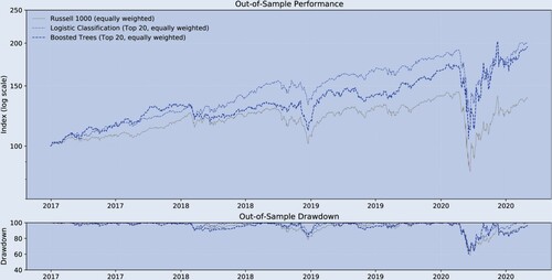
Table C1. Predicted vs. realized returns (robustness test B, out-of-sample).

Method	Measure	Entire sample	Top/Bottom 50	Top/Bottom 20	Top/Bottom 10
Logistic classification	Mean	0.04	0.07	0.08	0.1
	Median	0.04	0.08	0.09	0.1
	Max	0.34	0.58	0.71	0.81
	Min	−0.31	−0.57	−0.66	−0.8
	Std	0.11	0.18	0.22	0.27
Boosted trees	Mean	0.02	0.05	0.05	0.06
	Median	0.0	0.03	0.07	0.07
	Max	0.44	0.66	0.8	0.88
	Min	−0.24	−0.49	−0.64	−0.74
	Std	0.1	0.2	0.25	0.31

Notes: bi-weekly forecast horizon and rebalancing; in-sample period: 1995.12–2016.12; out-of-sample period: 2016.12–2020.08; Stock Sample: Russell 1000. This table shows the pooled correlations (across stocks and points in time) between predicted and subsequently realized returns.

Table C2. Performance indicators (robustness test B, out-of-sample).

	Indicator	2017	2018	2019	2020	Overall
Russell 1000 (eq w)	Return(%)	18.66	−8.96	29.92	−2.0	9.1
	Volatility(%)	8.14	16.09	13.56	47.27	23.32
	max Drawdown	−3.67	−21.54	−7.49	−41.67	−41.67
	Sharpe Ratio	2.29	−0.56	2.21	−0.04	0.39
	Return to $|$max Drawdown$|$	5.09	−0.42	4.0	−0.05	0.22
	Market Correlation	1.0	1.0	1.0	1.0	1.0
Logistic (Top 20, eq w)	Return(%)	25.57	9.61	32.78	9.38	20.82
	Volatility(%)	8.21	16.13	11.7	38.32	19.81
	max Drawdown	−2.52	−15.16	−5.23	−36.68	−36.68
	Sharpe Ratio	3.11	0.6	2.8	0.24	1.05
	Return to $|$max Drawdown$|$	10.14	0.63	6.27	0.26	0.57
	Market Correlation	0.8	0.91	0.82	0.92	0.86
Boosted T (Top 20, eq w)	Return(%)	31.84	−10.03	40.68	17.03	20.05
	Volatility(%)	10.17	16.18	14.7	54.72	26.49
	max Drawdown	−4.55	−18.06	−8.91	−39.66	−39.66
	Sharpe Ratio	3.13	−0.62	2.77	0.31	0.76
	Return to $|$max Drawdown$|$	7.0	−0.56	4.57	0.43	0.51
	Market Correlation	0.68	0.79	0.88	0.88	0.81

Notes: bi-weekly forecast horizon and rebalancing; in-sample period: 1995.12–2016.12; out-of-sample period: 2016.12–2020.08; Stock Sample: Russell 1000. This table shows a variety of performance measures for different trading strategies.

Appendix 3. Robustness: rebalancing and forecasting at alternative frequencies

As the third robustness test, we employ two alternative forecasting and rebalancing horizons: (i) monthly and (ii) weekly. Tables A4 and A5 are broadly in line with the corresponding table from the main text. As in the original table, these tables confirm that (i) Boosted Trees slightly outperform the Logistic approach in terms of mean out-of-sample correlation, (ii) the mean out-of-sample correlation for both the Logistic approach and Boosted Trees increases at the extremes, and (iii) the highest out-of-sample $R^2$ (the squared correlation) is less than 1% (Boosted Trees, Top/Bottom 10, Pearson: 0.07). Figures A3, A4 and tables A6, A7 show that the results from monthly rebalancing are broadly in line with their bi-weekly counterparts in the main text. Namely, the Logistic approach and Boosted Trees outperform the long-only benchmark both in terms of absolute and risk-adjusted returns.

Figure A3. Historical performance (robustness test C, out-of-sample, monthly).

Notes: monthly forecast horizon and rebalancing; in-sample period: 1995.12–2013.12; out-of-sample period: 2013.12–2020.08; Stock Sample: Russell 1000. This figure compares the performance of the different trading strategies.

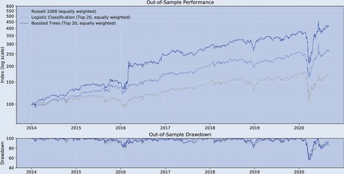
Figure A4. Performance indicators (robustness test C, out-of-sample, weekly).

Notes: weekly forecast horizon and rebalancing; in-sample period: 1995.12–2013.12; out-of-sample period: 2013.12–2020.08; Stock Sample: Russell 1000. This table shows a variety of performance measures for different trading strategies.

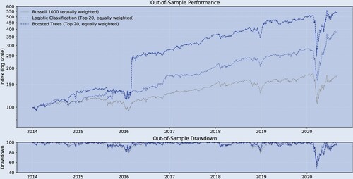
Table D1. Predicted vs. realized returns (robustness test C, out-of-sample, monthly.

Method	Measure	Entire sample	Top/Bottom 50	Top/Bottom 20	Top/Bottom 10
Logistic classification	Mean	0.03	0.04	0.04	0.04
	Median	0.03	0.04	0.05	0.04
	Max	0.29	0.52	0.72	0.81
	Min	−0.28	−0.48	−0.69	−0.79
	Std	0.09	0.18	0.24	0.3
Boosted trees	Mean	0.02	0.05	0.06	0.07
	Median	0.02	0.06	0.06	0.07
	Max	0.38	0.67	0.81	0.93
	Min	−0.38	−0.6	−0.71	−0.88
	Std	0.09	0.2	0.25	0.31

Notes: monthly forecast horizon and rebalancing; in-sample period: 1995.12–2013.12; out-of-sample period: 2013.12–2020.08; Stock Sample: Russell 1000. This table shows the pooled correlations (across stocks and points in time) between predicted and subsequently realized returns.

Table D2. Predicted vs. realized returns (robustness test C, out-of-sample, weekly).

Method	Measure	Entire sample	Top/Bottom 50	Top/Bottom 20	Top/Bottom 10
Logistic classification	Mean	0.02	0.04	0.05	0.05
	Median	0.02	0.04	0.05	0.06
	Max	0.31	0.56	0.7	0.89
	Min	−0.27	−0.49	−0.62	−0.77
	Std	0.09	0.17	0.23	0.29
Boosted trees	Mean	0.03	0.06	0.06	0.06
	Median	0.02	0.05	0.06	0.07
	Max	0.44	0.68	0.82	0.89
	Min	−0.36	−0.63	−0.72	−0.76
	Std	0.09	0.2	0.26	0.31

Notes: weekly forecast horizon and rebalancing; in-sample period: 1995.12–2013.12; out-of-sample period: 2013.12–2020.08; Stock Sample: Russell 1000. This table shows the pooled correlations (across stocks and points in time) between predicted and subsequently realized returns.

Table D3. Historical performance (robustness test C, out-of-sample, monthly).

	Indicator	2014	2015	2016	2017	2018	2019	2020	Overall
Russell 1000 (eq w)	Return(%)	11.2	−3.18	15.93	18.64	−9.01	29.78	−2.09	8.41
	Volatility(%)	12.35	15.44	16.44	8.13	16.04	13.53	46.75	19.81
	max Drawdown	−9.51	−13.48	−12.67	−3.68	−21.48	−7.44	−41.41	−41.41
	Sharpe Ratio	0.91	−0.21	0.97	2.29	−0.56	2.2	−0.04	0.42
	Return to $|$max Drawdown$|$	1.18	−0.24	1.26	5.07	−0.42	4.0	−0.05	0.2
	Market Correlation	1.0	1.0	1.0	1.0	1.0	1.0	1.0	1.0
Logistic (Top 20, eq w)	Return(%)	15.81	17.32	24.94	18.92	0.23	27.8	2.1	15.69
	Volatility(%)	11.69	14.51	16.87	9.71	14.88	9.8	42.79	18.39
	max Drawdown	−7.74	−7.51	−10.75	−5.24	−14.77	−4.45	−36.87	−37.14
	Sharpe Ratio	1.35	1.19	1.48	1.95	0.02	2.84	0.05	0.85
	Return to $|$max Drawdown$|$	2.04	2.31	2.32	3.61	0.02	6.25	0.06	0.42
	Market Correlation	0.86	0.89	0.86	0.81	0.87	0.81	0.87	0.85
Boosted T (Top 20, eq w)	Return(%)	31.82	12.35	63.99	17.54	−1.27	33.08	10.68	23.82
	Volatility(%)	11.54	15.25	33.12	12.08	16.64	15.65	50.19	23.88
	max Drawdown	−5.33	−9.64	−11.8	−10.05	−19.69	−8.84	−44.99	−44.99
	Sharpe Ratio	2.76	0.81	1.93	1.45	−0.08	2.11	0.21	1.0
	Return to $|$max Drawdown$|$	5.97	1.28	5.42	1.75	−0.06	3.74	0.24	0.53
	Market Correlation	0.87	0.89	0.85	0.73	0.89	0.89	0.85	0.85

Notes: monthly forecast horizon and rebalancing; in-sample period: 1995.12–2013.12; out-of-sample period: 2013.12–2020.08; Stock Sample: Russell 1000. This figure compares the performance of the different trading strategies.

Table D4. Performance indicators (robustness test C, out-of-sample, weekly).

	Indicator	2014	2015	2016	2017	2018	2019	2020	Overall
Russell 1000 (eq w)	Return(%)	11.46	−3.18	16.69	18.85	−8.77	29.73	−1.44	8.72
	Volatility(%)	12.42	15.52	16.47	8.14	16.12	13.59	47.63	20.06
	max Drawdown	−9.59	−13.63	−12.7	−3.68	−21.52	−7.55	−41.88	−41.88
	Sharpe Ratio	0.92	−0.2	1.01	2.31	−0.54	2.19	−0.03	0.43
	Return to $|$max Drawdown$|$	1.19	−0.23	1.31	5.13	−0.41	3.94	−0.03	0.21
	Market Correlation	1.0	1.0	1.0	1.0	1.0	1.0	1.0	1.0
Logistic (Top 20, eq w)	Return(%)	10.9	15.03	36.14	17.41	6.14	30.61	35.15	22.28
	Volatility(%)	11.96	15.89	18.18	10.04	15.96	13.41	49.58	20.83
	max Drawdown	−10.53	−12.25	−9.66	−5.56	−15.38	−6.52	−43.95	−43.95
	Sharpe Ratio	0.91	0.95	1.99	1.73	0.38	2.28	0.71	1.07
	Return to $|$max Drawdown$|$	1.03	1.23	3.74	3.13	0.4	4.69	0.8	0.51
	Market Correlation	0.86	0.86	0.81	0.77	0.89	0.78	0.9	0.84
Boosted T (Top 20, eq w)	Return(%)	31.67	0.31	109.82	30.52	2.2	36.55	6.83	28.78
	Volatility(%)	14.75	14.26	40.49	9.88	18.27	16.77	63.42	28.59
	max Drawdown	−9.38	−10.71	−12.84	−5.3	−17.43	−9.26	−52.02	−52.02
	Sharpe Ratio	2.15	0.02	2.71	3.09	0.12	2.18	0.11	1.01
	Return to $|$max Drawdown$|$	3.38	0.03	8.55	5.76	0.13	3.95	0.13	0.55
	Market Correlation	0.84	0.85	0.79	0.73	0.87	0.81	0.85	0.82

Notes: weekly forecast horizon and rebalancing; in-sample period: 1995.12–2013.12; out-of-sample period: 2013.12–2020.08; Stock Sample: Russell 1000. This table shows a variety of performance measures for different trading strategies.

Appendix 4. Robustness: alternative boosting parameters

As the fourth robustness test, we focus on the Boosting parameters. The Logistic approach's parameters are straightforward, but Boosting warrants a variety of additional tests. As there is no theoretical guidance on how to choose these parameters, we present the results for several ad-hoc choices. First, Parameters 1 reduces the subsample of predictors to 50% when constructing each tree. In the main text, each tree is constructed from the entire sample of predictors. Second, Parameters 2 reduces the subsample of predictors to 50% but increases the number of maximum leaves to 400 and sets the maximum tree depth to 20 (in the main text the tree depth is 10 and the maximum number of leaves is 100). Third, Parameters 3 reduces the subsample of predictors to 50% and increases the learning rate to 1 (in the main text the learning rate is 0.1), and uses standard random forests parameters otherwise.

Finally, Parameters Non-NaN runs Boosted Tress from an in-sample period that does not contain any NaNs.

Table A8 is broadly consistent with the corresponding table from the main text. Across Parameters 1, Parameters 2 and Parameters 3, (i) the mean out-of-sample correlation for Boosted Trees increases at the extremes and (ii) the highest out-of-sample $R^2$ (the squared correlation) is less than 1% (Boosted Trees, Top/Bottom 10, Param 1, Spearman: 0.10). Figure A5 and table A6 are also broadly in line with their counterparts in the main text. Under Parameters 1,2 and 3, Boosted Trees outperform the long-only benchmark both in terms of absolute and risk-adjusted returns. Under Parameters Non-NaN out-of-sample performance is also better than long-only and similar to those under Parameters 1,2 and 3.

Figure A5. Historical performance (robustness test D, out-of-sample).

Notes: bi-weekly forecast horizon and rebalancing; in-sample period: 1995.12–2013.12; out-of-sample period: 2013.12–2020.08; Stock Sample: Russell 1000. This figure compares the performance of the different trading strategies.

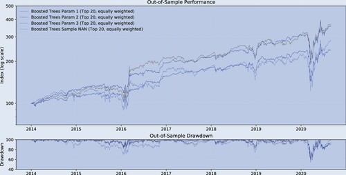
Figure A6. Performance indicators (robustness test D, out-of-sample).

Notes: bi-weekly forecast horizon and rebalancing; in-sample period: 1995.12–2013.12; out-of-sample period: 2013.12–2020.08; Stock Sample: Russell 1000. This table shows a variety of performance measures for different trading strategies.

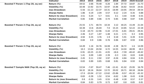
Table E1. Predicted vs. realized returns (robustness test D, out-of-sample).

Method	Measure	Entire sample	Top/Bottom 50	Top/Bottom 20	Top/Bottom 10
Boosted trees Param 1	Mean	0.03	0.06	0.08	0.09
	Median	0.02	0.06	0.08	0.1
	Max	0.46	0.64	0.81	0.93
	Min	−0.44	−0.62	−0.79	−0.82
	Std	0.1	0.2	0.26	0.32
Boosted trees Param 2	Mean	0.03	0.06	0.07	0.07
	Median	0.03	0.07	0.08	0.08
	Max	0.43	0.7	0.84	0.88
	Min	−0.49	−0.65	−0.76	−0.87
	Std	0.12	0.24	0.3	0.36
Boosted trees Param 3	Mean	0.02	0.04	0.04	0.04
	Median	0.02	0.04	0.04	0.03
	Max	0.41	0.67	0.82	0.83
	Min	−0.45	−0.62	−0.8	−0.83
	Std	0.12	0.25	0.3	0.37
Boosted trees Sample NAN	Mean	0.02	0.03	0.04	0.04
	Median	0.02	0.03	0.04	0.03
	Max	0.42	0.59	0.71	0.88
	Min	−0.27	−0.54	−0.58	−0.78
	Std	0.1	0.19	0.25	0.31

Notes: bi-weekly forecast horizon and rebalancing; in-sample period: 1995.12–2013.12; out-of-sample period: 2013.12–2020.08; Stock Sample: Russell 1000. This table shows the pooled correlations (across stocks and points in time) between predicted and subsequently realized returns.

Appendix 5. Robustness: alternative predictor normalization procedure

As the last robustness test, we employ an alternative normalization procedure for the predictor variables. In the main text, we impose a uniform distribution on the predictors enforcing equidistant steps between observations. A key advantage of this procedure is that it reduces the impact of outliers by effectively linearizing the predictors. In this appendix we will use the following formula to normalize the data: (A1) $x_i^{\prime }=\frac{x_i-x_i^{min}}{x_i^{max}-x_i^{min}},$(A1) where $x_i$ denotes predictor i. Table A9 is broadly in line with the corresponding table from the main text. As in the original table, this table confirms that (i) Boosted Trees outperforms the Logistic approach in terms of mean out-of-sample correlations, (ii) the out-of-sample correlation for both the Logistic approach and Boosted Trees increases at the extremes, and (iii) the highest out-of-sample $R^2$ (the squared correlation) is less than 1% (Boosted Trees, Top/Bottom 10, Spearman: 0.08). Figure A7 and table A10 are also broadly in line with their counterparts in the main text. Namely, the Logistic approach and Boosted Trees outperform the long-only benchmark both in terms of absolute and risk-adjusted returns most of the time. The Logistic approach is generally weaker than in the main text. This may be attributed to the fact that the normalization formula used here maintains the non-linearities which are difficult to capture with a linear approach.

Figure A7. Historical performance (robustness test E, out-of-sample).

Notes: bi-weekly forecast horizon and rebalancing; in-sample period: 1995.12–2013.12; out-of-sample period: 2013.12–2020.08; Stock Sample: Russell 1000. This figure compares the performance of the different trading strategies.

Table F1. Predicted vs. realized returns (robustness test E, out-of-sample).

Method	Measure	Entire sample	Top/Bottom 50	Top/Bottom 20	Top/Bottom 10
Logistic classification	Mean	0.01	0.02	0.03	0.03
	Median	0.01	0.02	0.03	0.04
	Max	0.37	0.72	0.81	0.87
	Min	−0.37	−0.67	−0.69	−0.84
	Std	0.12	0.23	0.27	0.31
Boosted trees	Mean	0.02	0.06	0.07	0.07
	Median	0.02	0.06	0.07	0.08
	Max	0.45	0.66	0.78	0.9
	Min	−0.44	−0.67	−0.78	−0.88
	Std	0.1	0.2	0.26	0.32

Notes: bi-weekly forecast horizon and rebalancing; in-sample period: 1995.12–2013.12; out-of-sample period: 2013.12–2020.08; Stock Sample: Russell 1000. This table shows the pooled correlations (across stocks and points in time) between predicted and subsequently realized returns.

Table F2. Performance indicators (robustness test E, out-of-sample).

	Indicator	2014	2015	2016	2017	2018	2019	2020	Overall
Russell 1000 (eq w)	Return(%)	11.42	−3.15	16.32	18.66	−8.96	29.92	−2.0	8.54
	Volatility(%)	12.41	15.48	16.53	8.14	16.09	13.56	47.27	19.97
	max Drawdown	−9.53	−13.62	−12.64	−3.67	−21.54	−7.49	−41.67	−41.67
	Sharpe Ratio	0.92	−0.2	0.99	2.29	−0.56	2.21	−0.04	0.43
	Return to $|$max Drawdown$|$	1.2	−0.23	1.29	5.09	−0.42	4.0	−0.05	0.2
	Market Correlation	1.0	1.0	1.0	1.0	1.0	1.0	1.0	1.0
Logistic (Top 20, eq w)	Return(%)	24.0	−4.91	22.15	13.65	3.17	30.96	7.4	13.87
	Volatility(%)	12.31	15.6	15.02	7.88	17.27	14.27	40.98	18.56
	max Drawdown	−6.45	−15.1	−7.0	−5.98	−17.01	−10.18	−31.29	−31.29
	Sharpe Ratio	1.95	−0.31	1.48	1.73	0.18	2.17	0.18	0.75
	Return to $|$max Drawdown$|$	3.72	−0.33	3.16	2.28	0.19	3.04	0.24	0.44
	Market Correlation	0.75	0.82	0.79	0.54	0.83	0.75	0.81	0.76
Boosted T (Top 20, eq w)	Return(%)	17.65	11.24	81.64	13.71	−0.76	24.63	20.77	23.3
	Volatility(%)	11.37	14.39	36.33	11.49	15.96	16.81	54.75	25.45
	max Drawdown	−7.22	−11.32	−13.92	−8.34	−19.62	−12.81	−40.65	−40.65
	Sharpe Ratio	1.55	0.78	2.25	1.19	−0.05	1.47	0.38	0.92
	Return to $|$max Drawdown$|$	2.44	0.99	5.87	1.64	−0.04	1.92	0.51	0.57
	Market Correlation	0.87	0.85	0.86	0.7	0.88	0.87	0.86	0.84

Notes: bi-weekly forecast horizon and rebalancing; in-sample period: 1995.12–2013.12; out-of-sample period: 2013.12–2020.08; Stock Sample: Russell 1000. This table shows a variety of performance measures for different trading strategies.

References

- Aghamolla, C. and Hashimoto, T., Information arrival, delay, and clustering in financial markets with dynamic freeriding. J. Financ. Econ., 2020, 138(1), 27–52. doi: https://doi.org/10.1016/j.jfineco.2020.04.011
- Alfarano, S., Lux, T. and Wagner, F., Estimation of agent-based models: the case of an asymmetric herding model. Comput. Econ., 2005, 26, 19–49. doi: https://doi.org/10.1007/s10614-005-6415-1
- Asness, C.S., Moskowitz, T.J. and Pedersen, L.H., Value and momentum everywhere. J. Finance, 2013, 68(3), 929–985. doi: https://doi.org/10.1111/jofi.12021
- Avery, C. and Zemsky, P., Multidimensional uncertainty and herd behavior in financial markets. Am. Econ. Rev., 1998, 88(4), 724–748.
- Banerjee, A.V., A simple model of herd behavior. Q. J. Econ., 1992, 107(3), 797–817. doi: https://doi.org/10.2307/2118364
- Barberis, N. and Shleifer, A., Style investing. J. Financ. Econ., 2003, 68(2), 161–199. doi: https://doi.org/10.1016/S0304-405X(03)00064-3
- Bendel, R.B. and Mickey, M.R., Population correlation matrices for sampling experiments. Commun. Statist. Simul. Comput., 1978, 7(2), 163–182. doi: https://doi.org/10.1080/03610917808812068
- Black, F., Noise. J. Finance, 1986, 41(3), 528–543. doi: https://doi.org/10.1111/j.1540-6261.1986.tb04513.x
- Bondt, W.F.M. De and Thaler, R., Does the stock market overreact? J. Finance, 1985, 40(3), 793–805. doi: https://doi.org/10.1111/j.1540-6261.1985.tb05004.x
- Bordalo, P., Gennaioli, N., La Porta, R. and Shleifer, A., Diagnostic expectations and stock returns. J. Finance, 2019, 74(6), 2839–2874. doi: https://doi.org/10.1111/jofi.12833
- Boswijk, H.P., Hommes, C.H. and Manzan, S., Behavioral heterogeneity in stock prices. J. Econ. Dyn. Control, 2007, 31(6), 1938–1970. 10th Workshop on Economic Heterogeneous Interacting Agents. doi: https://doi.org/10.1016/j.jedc.2007.01.001
- Boyer, B.H., Style-related comovement: Fundamentals or labels? J. Finance, 2011, 66(1), 307–332. doi: https://doi.org/10.1111/j.1540-6261.2010.01633.x
- Brock, W.A. and Hommes, C.H., A rational route to randomness. Econometrica, 1997, 65(5), 1059–1095. doi: https://doi.org/10.2307/2171879
- Campajola, C., Lillo, F. and Tantari, D., Unveiling the relation between herding and liquidity with trader lead-lag networks. Quant. Finance, 2020, 20(11), 1765–1778. doi: https://doi.org/10.1080/14697688.2020.1763442
- Chen, H.-S. and Sabherwal, S., Overconfidence among option traders. Rev. Financ. Econ., 2019, 37(1), 61–91. doi: https://doi.org/10.1002/rfe.1048
- Choi, N. and Sias, R.W., Institutional industry herding. J. Financ. Econ., 2009, 94(3), 469–491. doi: https://doi.org/10.1016/j.jfineco.2008.12.009
- Coval, J.D. and Shumway, T., Do behavioral biases affect prices? J. Finance., 2005, 60(1), 1–34. doi: https://doi.org/10.1111/j.1540-6261.2005.00723.x
- Davies, P.I. and Higham, N.J., Numerically stable generation of correlation matrices and their factors. BIT Numer. Math., 2000, 40(4), 640–651. doi: https://doi.org/10.1023/A:1022384216930
- De Long, J.B., Shleifer, A., Summers, L.H. and Waldmann, R.J., Noise trader risk in financial markets. J. Political Econ., 1990, 98(4), 703–738. doi: https://doi.org/10.1086/261703
- DellaVigna, S. and Pollet, J.M., Investor inattention and friday earnings announcements. J. Finance, 2009, 64(2), 709–749. doi: https://doi.org/10.1111/j.1540-6261.2009.01447.x
- Dennis, P.J. and Strickland, D., Who blinks in volatile markets, individuals or institutions? J. Finance, 2002, 57(5), 1923–1949. doi: https://doi.org/10.1111/0022-1082.00484
- Eyster, E., Rabin, M. and Vayanos, D., Financial markets where traders neglect the informational content of prices. J. Finance, 2019, 74(1), 371–399. doi: https://doi.org/10.1111/jofi.12729
- Fama, E.F., The behavior of stock-market prices. J. Bus., 1965, 38(1), 34–105. doi: https://doi.org/10.1086/294743
- Fama, E.F. and French, K.R., The cross-section of expected stock returns. J. Finance, 1992, 47(2), 427–465. doi: https://doi.org/10.1111/j.1540-6261.1992.tb04398.x
- Fama, E.F. and French, K.R., Dissecting anomalies with a five-factor model. Rev. Financ. Stud., 2016, 29(1), 69–103. doi: https://doi.org/10.1093/rfs/hhv043
- Farhi, E. and Gabaix, X., Rare disasters and exchange rates. Q. J. Econ., 2016, 131(1), 1–52. Lead Article. doi: https://doi.org/10.1093/qje/qjv040
- Fayyad, U.M. and Irani, K.B., Multi-interval discretization of continuous-valued attributes for classification learning. In Proceedings of the 13th International Joint Conference on Artificial Intelligence, 28 August–3 September, pp. 1022–1029, 1993 (IJCAI Organization: Chambéry).
- Freyberger, J., Neuhierl, A. and Weber, M., Dissecting characteristics nonparametrically. Rev. Financ. Stud., 2020, 33(5), 2326–2377. doi: https://doi.org/10.1093/rfs/hhz123
- Friedman, M., Essays in Positive Economics, 1953 (University of Chicago Press: Chicago).
- Froot, K.A, Scharftstein, D.S and Stein, J.C., Herd on the street: Informational inefficiencies in a market with short-term speculation. J. Finance, 1992, 47(4), 1461–1484. doi: https://doi.org/10.1111/j.1540-6261.1992.tb04665.x
- García, D., Sentiment during recessions. J. Finance, 2013, 68(3), 1267–1300. doi: https://doi.org/10.1111/jofi.12027
- Garcia, S., Luengo, J., Saez, J.A., Lopez, V. and Herrera, F., A survey of discretization techniques: Taxonomy and empirical analysis in supervised learning. IEEE Trans. Knowl. Data Eng., 2013, 25(4), 734–750. doi: https://doi.org/10.1109/TKDE.2012.35
- Grinblatt, M., Titman, S. and Wermers, R., Momentum investment strategies, portfolio performance, and herding: A study of mutual fund behavior. Am. Econ. Rev., 1995, 85(5), 1088–1105.
- Gu, S., Kelly, B. and Xiu, D., Empirical asset pricing via machine learning. Rev. Financ. Stud., 2020, 33(5), 2223–2273. doi: https://doi.org/10.1093/rfs/hhaa009
- Harvey, C.R., Liu, Y. and Zhu, H., … and the cross-section of expected returns. Rev. Financ. Stud., 2016, 29(1), 5–68. doi: https://doi.org/10.1093/rfs/hhv059
- Kolev, G.I. and Karapandza, R., Out-of-sample equity premium predictability and sample split–invariant inference. J. Banking Finance, 2017, 84, 188–201. doi: https://doi.org/10.1016/j.jbankfin.2016.07.017
- Kozak, S., Nagel, S. and Santosh, S., Shrinking the cross-section. J. Financ. Econ., 2020, 135(2), 271–292. doi: https://doi.org/10.1016/j.jfineco.2019.06.008
- Kukacka, J. and Barunik, J., Behavioural breaks in the heterogeneous agent model: The impact of herding, overconfidence, and market sentiment. Phys. A Stat. Mech. Appl., 2013, 392(23), 5920–5938. doi: https://doi.org/10.1016/j.physa.2013.07.050
- Lakonishok, J., Shleifer, A. and Vishny, R.W., Contrarian investment, extrapolation, and risk. J. Finance., 1994, 49(5), 1541–1578. doi: https://doi.org/10.1111/j.1540-6261.1994.tb04772.x
- Longstaff, F.A., How much can marketability affect security values? J. Finance, 1995, 50(5), 1767–1774. doi: https://doi.org/10.1111/j.1540-6261.1995.tb05197.x
- Lux, T. and Marchesi, M., Scaling and criticality in a stochastic multi-agent model of a financial market. Nature, 1999, 397, 498–500. doi: https://doi.org/10.1038/17290
- Mclean, R.D. and Pontiff, J., Does academic research destroy stock return predictability? J. Finance, 2016, 71(1), 5–32. doi: https://doi.org/10.1111/jofi.12365
- Moritz, B. and Zimmermann, T., Tree-based conditional portfolio sorts: The relation between past and future stock returns. SSRN Working Paper, 03, 2016.
- Nofsinger, J.R. and Sias, R.W., Herding and feedback trading by institutional and individual investors. J. Finance, 2002, 54(6), 2263–2295. doi: https://doi.org/10.1111/0022-1082.00188
- Novy-Marx, R. and Velikov, M., A taxonomy of anomalies and their trading costs. Rev. Financ. Stud., 2015, 29(1), 104–147. doi: https://doi.org/10.1093/rfs/hhv063
- Park, A. and Sabourian, H., Herding and contrarian behavior in financial markets. Econometrica, 2011, 79(4), 973–1026. doi: https://doi.org/10.3982/ECTA8602
- Peress, J. and Schmidt, D., Glued to the TV: Distracted noise traders and stock market liquidity. J. Finance, 2020, 75(2), 1083–1133. doi: https://doi.org/10.1111/jofi.12863
- Peter Chung, Y. and Thomas Kim, S., Extreme returns and herding of trade imbalances. Rev. Finance, 2017, 21(6), 2379–2399. doi: https://doi.org/10.1093/rof/rfx004
- Sandroni, A., Do markets favor agents able to make accurate predictions? Econometrica, 2000, 68(6), 1303–1341. doi: https://doi.org/10.1111/1468-0262.00163
- Sharpe, W.F., Capital asset prices: A theory of market equilibrium under conditions of risk. J. Finance, 1964, 19(3), 425–442.
- Shleifer, A. and Summers, L.H., The noise trader approach to finance. J. Econ. Perspect., 1990, 4(2), 19–33. doi: https://doi.org/10.1257/jep.4.2.19
- Shleifer, A. and Vishny, R.W., The limits of arbitrage. J. Finance, 1997, 52(1), 35–55. doi: https://doi.org/10.1111/j.1540-6261.1997.tb03807.x
- Shue, K. and Townsend, R., Can the market multiply and divide? Non-proportional thinking in financial markets. Working Paper 25751, April 2019. https://www.nber.org/papers/w25751
- Struck, C. and Cheng, E., Time-series momentum: A Monte Carlo approach. J. Financ. Data Sci., 2019, 1(4), 103–123. doi: https://doi.org/10.3905/jfds.2019.1.012
- Teo, M. and Woo, S.-J., Style effects in the cross-section of stock returns. J. Financ. Econ., 2004, 74(2), 367–398. doi: https://doi.org/10.1016/j.jfineco.2003.10.003
- Veldkamp, L.L., Media frenzies in markets for financial information. Am. Econ. Rev., 2006, 96(3), 577–601. doi: https://doi.org/10.1257/aer.96.3.577
- Westphal, R. and Sornette, D., Market impact and performance of arbitrageurs of financial bubbles in an agent-based model. J. Econ. Behav. Organ., 2020, 171, 1–23. doi: https://doi.org/10.1016/j.jebo.2020.01.004
- Xiong, W. and Yan, H., Heterogeneous expectations and bond markets. Rev. Financ. Stud., 2010, 23(4), 1433–1466. doi: https://doi.org/10.1093/rfs/hhp091
- Yan, H., Is noise trading cancelled out by aggregation? Manage. Sci., 2010, 56(7), 1047–1059. doi: https://doi.org/10.1287/mnsc.1100.1167