Optimal portfolio allocation and asset centrality revisited

Abstract

This paper revisits the relationship between eigenvector asset centrality and optimal asset allocation in a minimum variance portfolio. We show that the standard definition of eigenvector centrality is misleading when the adjacency matrix in a network can take negative values. This is, for example, the case when the network topology is induced by the correlation matrix between assets in a portfolio. To correct for this, we introduce the concept of positive and negative eigenvector centrality. Our results show that the loss function associated to the minimum variance portfolio is positively/negatively related to the positive and negative eigenvector centrality under short-selling constraints but cannot be generalized beyond that. Furthermore, in contrast to what is claimed in the related literature, this relationship does not imply any monotonic relationship between the centrality of an asset and its optimal portfolio allocation. These theoretical insights are illustrated empirically in a portfolio allocation exercise with assets from U.S. and U.K. financial markets.

Keywords:

• Eigenvector centrality
• Markowitz portfolio allocation
• Spectral decomposition
• Constant conditional correlation
• Dynamic conditional correlation

1. Introduction

Portfolio selection is a fundamental topic in financial economics and one of the leading applications of decision theory under uncertainty. Modern portfolio theory pioneered by Markowitz (1952, 1959) stresses the idea that portfolio diversification leads to a risk reduction. Agents minimize a loss function that is the sum of idiosyncratic risks given by the individual assets' variances and the correlation between the assets in the portfolio. In this problem the optimal asset allocation is determined by the inverse of the covariance matrix such that assets with large variances receive a lower allocation in the investment portfolio. The relationship between the assets in the portfolio characterized by the returns' correlations is an additional contributor to portfolio risk.

In this study, we embed the optimal portfolio allocation problem in a financial network. The nodes of the network are the financial assets comprising the portfolio and the links are the connections between the assets. We consider a weighted undirected network in which the relationship between the assets is driven by the cross-correlations between the log returns. Considering the relationship between assets in a portfolio as a financial network is not new. Measures of financial connectedness have been proposed in different areas of financial economics by Vandewalle et al. (2001), Tse et al. (2010), Billio et al. (2012), Diebold and Yilmaz (2009, 2012, 2014), Hautsch et al. (2015), Peralta and Zareei (2016) and Barigozzi and Brownlees (2018), among many others.

The notion of centrality aims to quantify the importance of certain nodes in a given network. In the same spirit of Peralta and Zareei (2016), we focus on the concept of eigenvector centrality and explore the relationship between asset centrality and portfolio risk. These authors attempt to formalize the results derived in Pozzi et al. (2013) and establish that optimal portfolio strategies should overweigh low-central securities and underweigh high central ones. These authors find that investors benefit from diversification by avoiding the allocation of wealth in assets that are central—using the correlation as the measure of association in the network. Our aim in this study is to shed further light on the relationship between the centrality of an asset in a portfolio and the overall risk of the portfolio. As a byproduct, we also explore the relationship between asset centrality and the optimal asset allocation in a global minimum variance portfolio. We focus on this optimization problem because it is a clean optimization problem that can be mathematically interpreted as a quadratic programming exercise. In financial terms, minimizing the portfolio variance is similar to optimizing the mean-variance portfolio strategy but avoids the estimation of the vector of expected returns.

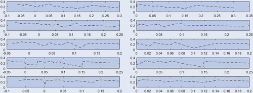
To understand in more detail the relationship between eigenvector centrality and the optimal allocation of an asset to an investment portfolio we construct an optimal portfolio with all the assets comprising the FTSE 100 Index using daily data over the period January 2011 to December 2018. The optimal allocation to each asset of the FTSE 100 Index is obtained from a minimum variance optimization function. Panel (a) of figure 1 reports the eigenvector centrality measure introduced by Bonacich (1972) as a function of the optimal portfolio weights for each of the 100 assets comprising the FTSE 100 Index. These results show a very weak decreasing relationship between eigenvector centrality and optimal portfolio weights. The range of the asset centrality statistic for the cross-section of assets in the Index is around 0.1 and the relationship fails to be monotonic. In Panel (b) we repeat the exercise but imposing short-selling constraints to the optimal portfolio allocation. In this case the relationship clearly fails to reflect the negative relationship between asset centrality and the corresponding allocation of the asset in the portfolio. To gain further insight into this relationship we repeat the exercise for random subsamples of stocks in the FTSE 100 Index. We divide the 100 assets comprising the financial index into five random subsamples of stock returns with 20 assets each and without replacement such that all assets in the FTSE 100 Index are represented in one and only one of the portfolios. The minimum variance optimal portfolio weights on the assets are ranked from minimum to maximum for each of these portfolios and the associated centrality measures are plotted in figure 2. The left panel of this figure reports the centrality of assets as a function of the weights under no short-selling constraints and the right panel reports the centrality measure as a function of the weights under short-selling constraints. Both sets of results fail to report a negative relationship between asset centrality and the portfolio allocation. These empirical insights suggest that such relationship obtained in related studies may not exist and be an artifact of the sample period or the presence of outlying observations in the datasets under study.

Figure 1. FTSE 100 Index. Centrality measures and portfolio weights. Panel (a) reports the relationship between asset centrality and the portfolio weights. To do this, the weights allocated to the assets comprising the FTSE 100 Index under the global minimum variance portfolio, see (2(2) ${\mathbf{w}}^{\ast }=\frac{{\mathbf{\Sigma }}^{-1}\mathbf{1}}{{\mathbf{1}}^{\mathrm{\prime }}{\mathbf{\Sigma }}^{-1}\mathbf{1}}.$(2) ), are ranked from smallest to largest and the associated centrality measure (9(9) $v_i={\overline{\omega }}^{-1}\sum _{j=1}^n{\mathrm{\Omega }}_{ij}{v}_j,$(9) ) is plotted. Panel (b) reports the relationship between asset centrality and the portfolio weights under short-selling constraints $\mathbf{w}\ge 0$.

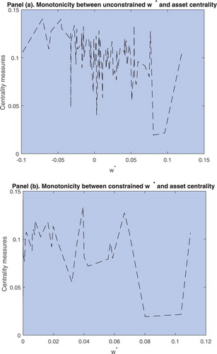
Figure 2. Random subsample of FTSE 100 Index. Centrality measures and portfolio weights. Each row contains a random subsample of 20 stock returns from the FTSE 100 Index such that the five rows span all the assets in the FTSE 100 Index. The left panel reports the relationship between asset centrality and the portfolio weights under the absence of short-selling constraints and the right panel reports such relationship imposing short-selling constraints ($\mathbf{w}\ge 0$).

In addition, standard eigenvector centrality measures, see Bonacich (1972), may not be suitable for measuring the centrality of an asset in a portfolio. In Markowitz's portfolio optimization context, the adjacency matrix is characterized by the correlation matrix. In contrast to standard formulations of the adjacency matrix in social and financial networks, this matrix contains positive and negative values that yield eigenvector centrality measures that can be negative. Moreover, the eigenvector centrality measures can produce misleading results if the positive and negative correlations across assets cancel out. In this case, the corresponding centrality measure can give values close to zero even for assets that are highly connected to the other assets in the portfolio. To correct for this, we extend the concept of eigenvector centrality to consider positive and negative eigenvector centrality measures separately. We achieve this by decomposing the correlation matrix in a diagonal matrix of ones and two complementary adjacency matrices. Each of these matrices contains the positive and negative correlations between the assets separately. Both matrices are symmetric accommodating a spectral decomposition. The positive and negative centrality measures are defined using the eigenvectors and eigenvalues of these spectral decompositions.

We use these definitions to explore theoretically and empirically the relationship between positive and negative eigenvector centrality and portfolio risk. Under short-selling constraints, we find a positive/negative monotonic relationship between the loss function characterizing the optimal minimum variance portfolio allocation and positive/negative centrality. This relationship vanishes as the short-selling condition is relaxed. Furthermore, in contrast to previous studies such as Pozzi et al. (2013) and Peralta and Zareei (2016), we find that, in general, there does not exist a monotonic decreasing relationship between asset centrality and the corresponding allocation of the assets to the portfolio. This result is shown theoretically and empirically independently of whether short-selling restrictions are imposed or not. Our theoretical results provide a correction of Proposition 1 and Corollary 1 of Peralta and Zareei (2016) and avoid imposing unrealistic assumptions on the maximum eigenvalue of the correlation matrix.

These theoretical insights are illustrated empirically with data from U.S. stock markets. We consider daily log returns on eight assets obtained from the Federal Reserve Bank of St Louis Database over the period 1 January 2011 to 29 May 2020. These assets are the CBOE Gold ETF Volatility Index, the U.S./Euro Foreign Exchange Rate, the Dow Jones Industrial Average, the Nasdaq 100 Index, the CBOE Russell 2000 Volatility Index, the S$\mathrm{\&}$P 500 Index, the CBOE Volatility Index (VIX), and the Willshire 5000 Price Index. Financial indexes are positively cross-correlated and negatively correlated to the volatility indexes. In this setting, we show that positive and negative centrality capture different dimensions of asset centrality. The standard eigenvector centrality measure proposed in Bonacich (1972) is different from these two centrality measures although it is positively correlated to the positive eigenvector centrality. Financial indexes are highly central with regards to the positive centrality measure whereas volatility indexes are in the periphery of the network. This result is due to the presence of positive correlations between the four financial indexes: Dow Jones Industrial Average, Nasdaq 100 Index, S$\mathrm{\&}$P 500 Index and the Willshire 5000 Price Index, and their negative correlation to the volatility indexes. The volatility indexes are central using the negative centrality measure. This is due to the negative correlations between these assets and the conventional financial indexes. The latter assets also exhibit a high value of the negative centrality statistic meaning that conventional financial indexes exhibit high correlation (positive and negative) with all the remaining assets in the portfolio.

The analysis of the relationship between asset centrality and portfolio allocation provides empirical support to our theoretical result showing that no monotonic relationship exists between both variables. We also confirm empirically that both centrality measures move together under small variations in the optimal portfolio weights. We extend the static case to the dynamic case by considering constant conditional correlation (CCC) models introduced in Bollerslev (1990), and dynamic conditional correlation (DCC) models developed by Engle (2002). Our empirical findings confirm the theoretical features of the models, namely, both positive and negative centrality measures are constant over the evaluation period for the CCC model. Interestingly, there is no much variation in asset centrality for the DCC model despite the flexibility offered by the latter specification. The centrality of the U.S./Euro Foreign Exchange Rate exhibits more variation than the centrality of the remaining assets. Overall, we find that modelling the dynamics of the multivariate volatility process using a DCC model does not alter significantly the centrality measures between the assets providing empirical support to the CCC specification with respect to the DCC model.

The rest of the paper is organized as follows. Section 2 reviews the theoretical background and introduces the main results of the paper. Section 3 presents an empirical application to a set of U.S. assets and assesses empirically the relationship between asset centrality and the optimal portfolio weights. Section 4 concludes. Proofs of the main results of the study are found in a mathematical appendix.

2. Optimal asset allocation

In this section, we review the minimum variance optimal portfolio allocation problem developed by Markowitz (1952) and introduce the main results of the study.

2.1. Minimum variance portfolio optimization

The traditional portfolio optimization theory in the simplest case considers the minimization of portfolio variance without any further restriction on portfolio's expected return. More formally, let $\mathbf{r}=[r_1,\dots ,r_n{]}^{\mathrm{\prime }}$ be the vector of asset returns with expected values denoted as $\left[\mathbb{E}\right(r_1),\dots ,\mathbb{E}(r_n){]}^{\mathrm{\prime }}$, and covariance matrix denoted as $\mathbf{\Sigma }\equiv \mathrm{C}\mathrm{o}\mathrm{v}\left(\mathbf{r}\right)=\mathbb{E}\left(\mathbf{r}{\mathbf{r}}^{\mathrm{\prime }}\right)-\mathbb{E}\left(\mathbf{r}\right)\mathbb{E}(\mathbf{r}{)}^{\mathrm{\prime }}$. The diagonal elements of this matrix contain the idiosyncratic variance terms ${\sigma }_i^2$ and the off-diagonal terms contain the covariance terms ${\sigma }_{ij}$ between the assets.

Let $r^p={\mathbf{w}}^{\mathrm{\prime }}\mathbf{r}$ denote the return on a portfolio of n assets, with $\mathbf{w}=[w_1,\dots ,w_n{]}^{\mathrm{\prime }}$ the vector of portfolio weights representing the allocation of assets to the portfolio. The global minimum variance optimization problem developed by Markowitz (1952) is (1) $\underset{\mathbf{w}\in {\mathbb{R}}^n}{\mathrm{a}\mathrm{r}\mathrm{g}\mathrm{m}\mathrm{i}\mathrm{n}}Q(\mathbf{\Sigma },\mathbf{w})\text{subject to }{\mathbf{w}}^{\mathrm{\prime }}\mathbf{1}=1,$(1) with $Q(\mathbf{\Sigma },\mathbf{w})={\mathbf{w}}^{\mathrm{\prime }}\mathbf{\Sigma }\mathbf{w}$ the portfolio variance. The first-order conditions to the minimization problem yield the optimal portfolio allocation given by the following vector of weights (2) ${\mathbf{w}}^{\ast }=\frac{{\mathbf{\Sigma }}^{-1}\mathbf{1}}{{\mathbf{1}}^{\mathrm{\prime }}{\mathbf{\Sigma }}^{-1}\mathbf{1}}.$(2) Markowitz (1952) also considers the extension of this portfolio allocation problem to the mean-variance case. The results for this case follow similarly after suitable modifications of the algebra and are omitted for space constraints.

The aim of this paper is to study the role of asset centrality in the portfolio allocation problem. To do so we revisit the standard minimum variance portfolio optimization problem from a financial network perspective. The matrix $\mathbf{\Sigma }$ can be decomposed as $\mathbf{\Sigma }=\mathbf{\Delta }\mathbf{\Omega }\mathbf{\Delta }$, with $\mathbf{\Omega }$ the correlation matrix of returns and $\mathbf{\Delta }$ a diagonal matrix whose ith-main diagonal element is ${\sigma }_i$. Furthermore, by construction, the correlation matrix $\mathbf{\Omega }$ is symmetric and positive definite. The diagonal of the matrix is a vector of ones and the off-diagonal terms are the correlation parameters ${\rho }_{ij}$. The symmetry of $\mathbf{\Omega }$ entails the spectral decomposition $\mathbf{\Omega }=\mathbf{U}{\mathbf{D}}_{\omega }{\mathbf{U}}^{\mathrm{\prime }}$, with $\mathbf{U}$ an $n\times n$ orthonormal matrix such that ${\mathbf{U}}^{\mathrm{\prime }}={\mathbf{U}}^{-1}$ that contains the linearly independent eigenvectors of $\mathbf{\Omega }$ and ${\mathbf{D}}_{\omega }$ an $n\times n$ diagonal matrix with the corresponding eigenvalues ${\omega }_k$, with $k=1,\dots ,n$. The eigenvalues of the risk matrix $\mathbf{\Omega }$ can be expressed as a function of the elements of the correlation matrix as (3) ${\omega }_k=\sum _{i=1}^n{u}_{ik}^2+\sum _{i=1}^n\sum _{\begin{array}{c}j\ne i\\ j=1\end{array}}^n{u}_{ik}{u}_{jk}{\rho }_{ij},$(3) with $u_{ij}$ the $i^{th}$ component of the $j^{th}$ eigenvector of the matrix $\mathbf{\Omega }\in {\mathbb{R}}^{n\times n}$. By definition of the matrix $\mathbf{U}$, it holds that $\sum _{i=1}^n{u}_{ik}^2=1$ such that ${\omega }_k=1+\sum _{i=1}^n\sum _{\begin{array}{c}j\ne i\\ j=1\end{array}}^n{u}_{ik}{u}_{jk}{\rho }_{ij}$. From this expression, it follows that the eigenvalues of the risk matrix $\mathbf{\Sigma }$, denoted as ${\gamma }_k$, can be expressed in terms of the variances and covariances as (4) ${\gamma }_k=\sum _{i=1}^n{u}_{ik}^2{\sigma }_i^2+\sum _{i=1}^n\sum _{\begin{array}{c}j\ne i\\ j=1\end{array}}^n{u}_{ik}{u}_{jk}{\sigma }_{ij}.$(4) The eigenvectors of both matrices $\mathbf{\Sigma }$ and $\mathbf{\Omega }$ are obtained from the matrix $\mathbf{U}$. By construction, both matrices are positive definite implying that ${\omega }_k$ and ${\gamma }_k$ are strictly greater than zero for $k=1,\dots ,n$.

2.2. Optimal portfolio weights and network centrality

The notion of centrality aims to quantify the importance of certain nodes in a given network. The literature on social interactions and networks has proposed several measures to capture the interdependence between individuals in a network. Intuitive measures of network centrality are given by Kratz's centrality measure, see Katz (1953), and PageRank used by Google in their famous search engine. One of the main measures for capturing the centrality of an individual in a network is the eigenvector centrality, firstly introduced in Bonacich (1972).

In this paper, the connections between the assets in a network are determined by the correlation matrix. This matrix is interpreted as an adjacency matrix in which the magnitude of the correlation parameters between the assets determines the strength of the relationship. We focus on the minimum variance portfolio optimization problem outlined in the previous subsection.

Let $\mathbf{\Omega }={\mathbf{I}}_n+\mathbf{\Lambda }$, with ${\mathbf{I}}_n$ the identity matrix and $\mathbf{\Lambda }$ an adjacency matrix that is symmetric and defined by a vector of zeros in the diagonal terms and the off-diagonal terms are the same of the risk matrix $\mathbf{\Omega }$, i.e. ${\mathrm{\Lambda }}_{ij}={\rho }_{ij}$ for $i\ne j$. The network is weighted because the connections between the assets are determined by the correlation matrix and undirected because the matrix is symmetric. The symmetry of the adjacency matrix entails the spectral decomposition $\mathbf{\Lambda }=\mathbf{U}{\mathbf{D}}_{\lambda }{\mathbf{U}}^{\mathrm{\prime }}$, where $\mathbf{U}$ is the same matrix as in the spectral decomposition of $\mathbf{\Omega }$. Both matrices $\mathbf{\Lambda }$ and $\mathbf{\Omega }$ have the same eigenvectors. Similarly, the eigenvalues of these matrices satisfy that ${\omega }_k=1+{\lambda }_k$ for $k=1,\dots ,n$. This property can be shown from expression (3(3) ${\omega }_k=\sum _{i=1}^n{u}_{ik}^2+\sum _{i=1}^n\sum _{\begin{array}{c}j\ne i\\ j=1\end{array}}^n{u}_{ik}{u}_{jk}{\rho }_{ij},$(3) ) and the decomposition of the eigenvalues of the adjacency matrix $\mathbf{\Lambda }$ as a function of the correlation parameters. More formally, (5) ${\lambda }_k=\sum _{i=1}^n\sum _{\begin{array}{c}j\ne i\\ j=1\end{array}}^n{u}_{ik}{u}_{jk}{\rho }_{ij}.$(5) The correlation matrix is positive definite implying that ${\lambda }_k>-1$ for $k=1,\dots ,n$. Under these conditions, the quadratic form given by the portfolio variance can be expressed as (6) $Q(\mathbf{\Sigma },\mathbf{w})={\mathbf{w}}^{\mathrm{\prime }}\mathbf{\Sigma }\mathbf{w}={\tilde{\mathbf{w}}}^{\mathrm{\prime }}\mathbf{\Omega }\tilde{\mathbf{w}}={\tilde{\mathbf{w}}}^{\mathrm{\prime }}\mathbf{\Lambda }\tilde{\mathbf{w}}+{\tilde{\mathbf{w}}}^{\mathrm{\prime }}\tilde{\mathbf{w}},$(6) with $\tilde{\mathbf{w}}=\mathbf{\Delta }\mathbf{w}$. This decomposition shows that the portfolio loss function can be divided into a component that is driven by the adjacency matrix $\mathbf{\Lambda }$ and the idiosyncratic risks ${\sigma }_i^2$ weighted by the portfolio weights $w_i$.

In what follows, we investigate the contribution of the centrality of an asset to the loss function $Q(\mathbf{\Sigma },\mathbf{w})$. To do so, we decompose the adjacency matrix as $\mathbf{\Lambda }={\mathbf{\Lambda }}_1-{\mathbf{\Lambda }}_2$, with ${\mathbf{\Lambda }}_1=\mathbf{\Lambda }\otimes \mathbf{1}(\mathbf{\Lambda }>0)$ containing the positive correlation parameters and ${\mathbf{\Lambda }}_2=-\mathbf{\Lambda }\otimes \mathbf{1}(\mathbf{\Lambda }<0)$ the matrix containing the negative correlation parameters; $\mathbf{1}(\mathbf{\Lambda }<0)$ is an indicator function that is applied elementwise to all the members of the matrix. This function takes a value of one if the argument is true and zero otherwise; ⊗ denotes the Hadamard product that denotes element by element multiplication. The spectral decomposition of $\mathbf{\Lambda }$ implies that ${\mathbf{D}}_{\lambda }={\mathbf{U}}^{\mathrm{\prime }}\mathbf{\Lambda }\mathbf{U}={\mathbf{\Lambda }}_1^{\ast }-{\mathbf{\Lambda }}_2^{\ast }$, with ${\mathbf{\Lambda }}_1^{\ast }={\mathbf{U}}^{\mathrm{\prime }}{\mathbf{\Lambda }}_1\mathbf{U}$ and ${\mathbf{\Lambda }}_2^{\ast }={\mathbf{U}}^{\mathrm{\prime }}{\mathbf{\Lambda }}_2\mathbf{U}$. Furthermore, the symmetry of ${\mathbf{\Lambda }}_1$ and ${\mathbf{\Lambda }}_2$ implies that ${\mathbf{\Lambda }}_1^{\ast }={\tilde{\mathbf{U}}}_1{\mathbf{D}}_{{\lambda }_1}{\tilde{\mathbf{U}}}_1^{\mathrm{\prime }}$ and ${\mathbf{\Lambda }}_2^{\ast }={\tilde{\mathbf{U}}}_2{\mathbf{D}}_{{\lambda }_2}{\tilde{\mathbf{U}}}_2^{\mathrm{\prime }}$, with ${\tilde{\mathbf{U}}}_1={\mathbf{U}}^{\mathrm{\prime }}{\mathbf{U}}_1$ and ${\tilde{\mathbf{U}}}_2={\mathbf{U}}^{\mathrm{\prime }}{\mathbf{U}}_2$; ${\mathbf{D}}_{{\lambda }_1}$ and ${\mathbf{D}}_{{\lambda }_2}$ are two diagonal matrices with main diagonal given by the eigenvalues of ${\mathbf{\Lambda }}_1$ and ${\mathbf{\Lambda }}_2$, respectively. The relationship between the eigenvalues of the adjacency matrix $\mathbf{\Lambda }$ and the eigenvalues of ${\mathbf{\Lambda }}_1$ and ${\mathbf{\Lambda }}_2$ is given by the following expression: (7) ${\mathbf{D}}_{\lambda }={\tilde{\mathbf{U}}}_1{\mathbf{D}}_{{\lambda }_1}{\tilde{\mathbf{U}}}_1^{\mathrm{\prime }}-{\tilde{\mathbf{U}}}_2{\mathbf{D}}_{{\lambda }_2}{\tilde{\mathbf{U}}}_2^{\mathrm{\prime }}.$(7) Then, (8) ${\lambda }_k=\sum _{i=1}^n{\lambda }_{1i}{\left(\sum _{j=1}^n{u}_{jk}{u}_{1,ji}\right)}^2-\sum _{i=1}^n{\lambda }_{2i}{\left(\sum _{j=1}^n{u}_{ji}{u}_{2,ji}\right)}^2,$(8) with $u_{1,ij}$ and $u_{2,ij}$ the elements of the matrices ${\mathbf{U}}_1$ and ${\mathbf{U}}_2$, respectively.

The notion of centrality quantifies the influence of certain nodes in a given network. There are several measurements in the literature each corresponding to a specific definition of centrality. We focus on eigenvector centrality; see Bonacich (1972) and Katz (1953). Peralta and Zareei (2016), in a related study, adapt the definition of eigenvector centrality introduced by these authors to a portfolio allocation context. More specifically, eigenvector centrality is defined as (9) $v_i={\overline{\omega }}^{-1}\sum _{j=1}^n{\mathrm{\Omega }}_{ij}{v}_j,$(9) with ${\mathrm{\Omega }}_{ij}$ the elements of the correlation matrix $\mathbf{\Omega }$ and $\overline{\omega }=max\{{\omega }_1,\dots ,{\omega }_n\}$. This definition of asset centrality in a portfolio provides an association measure between assets in the portfolio. The connectivity in the network is induced by the correlation matrix but, in contrast to considering pairwise correlations to assess the linear dependence between the assets, see Billio et al. (2012), the centrality measure (9(9) $v_i={\overline{\omega }}^{-1}\sum _{j=1}^n{\mathrm{\Omega }}_{ij}{v}_j,$(9) ) is driven by the largest eigenvalue of the spectral decomposition of the adjacency matrix. This eigenvalue, $\overline{\omega }$, and associated eigenvector, $\mathbf{v}$, contain most of the relevant information on the correlation matrix as known from principal components analysis. Asset centrality $v_i$ is proportional to the weighted sum of the centralities of neighbors of the asset with the corresponding elements of the correlation matrix as the weighting factors.

In contrast to the literature on social networks, the elements of the adjacency matrices $\mathbf{\Omega }$ and $\mathbf{\Lambda }$ can take positive and negative values implying that the corresponding centrality measure (9(9) $v_i={\overline{\omega }}^{-1}\sum _{j=1}^n{\mathrm{\Omega }}_{ij}{v}_j,$(9) ) may take negative values. In these cases the centrality measure is not well defined. More importantly, there can be cases where the positive and negative correlations between the assets cancel out implying a null centrality statistic (9(9) $v_i={\overline{\omega }}^{-1}\sum _{j=1}^n{\mathrm{\Omega }}_{ij}{v}_j,$(9) ) even if the asset is related to all the other assets in the portfolio. To overcome this issue, we define two centrality measures (positive and negative centrality) for a symmetric adjacency matrix $\mathbf{\Lambda }$. The rationale for splitting $\mathbf{\Lambda }$ in two as discussed above is the possibility of defining two centrality measures that are defined over the positive real line. More formally,

Definition 1

Let $\mathbf{\Lambda }={\mathbf{\Lambda }}_1-{\mathbf{\Lambda }}_2$ be an adjacency matrix as defined above. Then, positive centrality is defined by a vector ${\mathbf{v}}^p=[v_1^p,\dots ,v_n^p]$ such that (10) $v_i^p={\overline{\lambda }}_1^{-1}\sum _{j=1}^n{\mathrm{\Lambda }}_{1,ij}{v}_j^p,$(10) where ${\overline{\lambda }}_1=max({\lambda }_{11},\dots ,{\lambda }_{1n})$ is the largest eigenvalue of ${\mathbf{\Lambda }}_1$ and ${\mathrm{\Lambda }}_{1,ij}$ are the elements of such matrix. Similarly, negative centrality is defined by a vector ${\mathbf{v}}^n=[v_1^n,\dots ,v_n^n]$ such that (11) $v_i^n={\overline{\lambda }}_2^{-1}\sum _{j=1}^n{\mathrm{\Lambda }}_{2,ij}{v}_j^n,$(11) where ${\overline{\lambda }}_2=max({\lambda }_{21},\dots ,{\lambda }_{2n})$ is the largest eigenvalue of ${\mathbf{\Lambda }}_2$ and ${\mathrm{\Lambda }}_{2,ij}$ are the elements of such matrix.

Both centrality measures are defined over the positive real line for all assets in the portfolio if the maximum eigenvalue of each matrix is positive. Thus, for each asset, we obtain a pair of centrality measures $(v_i^p,v_i^n)$ that allow us to rank assets in the portfolio as a function of their position in the financial network. Furthermore, the centrality measures proposed above are the eigenvectors of the matrices ${\mathbf{\Lambda }}_1$ and ${\mathbf{\Lambda }}_2$ corresponding to the respective largest eigenvalues. This is so because ${\overline{\lambda }}_1{\mathbf{v}}^p={\mathbf{\Lambda }}_1{\mathbf{v}}^p$ and ${\overline{\lambda }}_2{\mathbf{v}}^n={\mathbf{\Lambda }}_2{\mathbf{v}}^n$. Throughout the text, we will assume that the first eigenvector of matrix ${\mathbf{U}}_1$ is associated to ${\overline{\lambda }}_1$ and, therefore, it defines the positive centrality statistic. Similarly, the first eigenvector of matrix ${\mathbf{U}}_2$ is associated to ${\overline{\lambda }}_2$ and, therefore, it defines the negative centrality statistic.

The following result shows that the eigenvector centrality measures are common across location-scale transformations of the adjacency matrix $\mathbf{\Lambda }$. More formally,

Proposition 1

Let $\mathbf{\Theta }=c_1{\mathbf{I}}_n+c_2\mathbf{\Lambda }$ be a location-scale transformation of the adjacency matrix $\mathbf{\Lambda }$ characterized by the constants $c_1\in \mathbb{R}$ and $c_2>0$. Then, the centrality measures $(v_i^p,v_i^n)$ of $\mathbf{\Lambda }$ are also the centrality measures of $\mathbf{\Theta }$.

In particular, for $c_1=c_2=1$, this result implies that the centrality measures $(v_i^p,v_i^n)$ of the correlation matrix $\mathbf{\Omega }$ are the same centrality measures of the adjacency matrix $\mathbf{\Lambda }$. The above proposition also implies the following result.

Lemma 1

The centrality of an asset as defined in (9(9) $v_i={\overline{\omega }}^{-1}\sum _{j=1}^n{\mathrm{\Omega }}_{ij}{v}_j,$(9) ) and positive centrality as defined in (10(10) $v_i^p={\overline{\lambda }}_1^{-1}\sum _{j=1}^n{\mathrm{\Lambda }}_{1,ij}{v}_j^p,$(10) ) are equal measures $(v_i\equiv v_i^p)$ for each asset $i=1,\dots ,n$ in the portfolio if ${\mathbf{\Lambda }}_{\mathbf{2}}$ is an empty matrix, that is, if the off-diagonal elements of the correlation matrix $\mathbf{\Omega }$ are all positive.

The latter result presents the conditions under which the standard centrality measure used in the literature is equal to the positive centrality measure defined herein. Otherwise, for correlation matrices with negative entries, these measures diverge.

The following result derives the relationship between asset centrality $(v_i^p,v_i^n)$ and portfolio risk. Expression (6(6) $Q(\mathbf{\Sigma },\mathbf{w})={\mathbf{w}}^{\mathrm{\prime }}\mathbf{\Sigma }\mathbf{w}={\tilde{\mathbf{w}}}^{\mathrm{\prime }}\mathbf{\Omega }\tilde{\mathbf{w}}={\tilde{\mathbf{w}}}^{\mathrm{\prime }}\mathbf{\Lambda }\tilde{\mathbf{w}}+{\tilde{\mathbf{w}}}^{\mathrm{\prime }}\tilde{\mathbf{w}},$(6) ) shows that portfolio risk $Q(\mathbf{\Sigma },\mathbf{w})$ can be decomposed into two components: ${\tilde{\mathbf{w}}}^{\mathrm{\prime }}\mathbf{\Lambda }\tilde{\mathbf{w}}$ and ${\tilde{\mathbf{w}}}^{\mathrm{\prime }}\tilde{\mathbf{w}}$. We proceed to study the relationship between the centrality measures $(v_i^p,v_i^n)$ and ${\tilde{\mathbf{w}}}^{\mathrm{\prime }}\mathbf{\Lambda }\tilde{\mathbf{w}}$. The second component given by ${\tilde{\mathbf{w}}}^{\mathrm{\prime }}\tilde{\mathbf{w}}$ only depends on the diagonal elements of the risk matrix $\mathbf{\Sigma }$ that contain the idiosyncratic risks. Let $\mathbf{0}$ be a $n\times 1$ vector of zeros.

Proposition 2

Under short-selling constraints, there is a positive monotonic relationship between the loss function ${\tilde{\mathbf{w}}}^{\mathrm{\prime }}\mathbf{\Lambda }\tilde{\mathbf{w}}$ and the positive centrality $v_i^p$ of each asset $i=1,\dots ,n$ in the portfolio.

Similar results can be obtained for the analysis of negative centrality of an asset. In particular,

Proposition 3

Under short-selling constraints, there is a negative monotonic relationship between the loss function ${\tilde{\mathbf{w}}}^{\mathrm{\prime }}\mathbf{\Lambda }\tilde{\mathbf{w}}$ and the negative centrality $v_i^n$ of each asset $i=1,\dots ,n$ in the portfolio.

More generally, under the absence of short-selling constraints, the relationship between the loss function ${\tilde{\mathbf{w}}}^{\mathrm{\prime }}\mathbf{\Lambda }\tilde{\mathbf{w}}$ and asset centrality is not monotonic. We are now ready to introduce the main result of this section, namely, the absence of a monotonic decreasing relationship between the centrality measures and the optimal allocation of the assets to the portfolio. This insight contrasts with recent results in the related literature such as Pozzi et al. (2013) and Peralta and Zareei (2016). These authors show that optimal strategies should underweigh the allocation to high central assets and overweigh the allocation to low central assets. In what follows, we challenge these conclusions. In particular, using similar methods to Peralta and Zareei (2016), we show that the relationship between the optimal portfolio allocation of a minimum variance portfolio and asset centrality is not monotonic. To formally show this, we need the following results. The eigenvalues ${\omega }_k$ of the correlation matrix $\mathbf{\Omega }$ satisfy that (12) $\begin{array}{rl}{\omega }_k& =1+{\overline{\lambda }}_1{\left(\sum _{j=1}^n{u}_{jk}{v}_j^p\right)}^2-{\overline{\lambda }}_2{\left(\sum _{j=1}^n{u}_{jk}{v}_j^n\right)}^2\\ & +\sum _{i=2}^n\left[{\lambda }_{1i}{\left(\sum _{j=1}^n{u}_{jk}{u}_{1,ji}\right)}^2-{\lambda }_{2i}{\left(\sum _{j=1}^n{u}_{jk}{u}_{2,ji}\right)}^2\right].\end{array}$(12) This result is immediate from expression (8(8) ${\lambda }_k=\sum _{i=1}^n{\lambda }_{1i}{\left(\sum _{j=1}^n{u}_{jk}{u}_{1,ji}\right)}^2-\sum _{i=1}^n{\lambda }_{2i}{\left(\sum _{j=1}^n{u}_{ji}{u}_{2,ji}\right)}^2,$(8) ) and noting that the first eigenvector of the matrices ${\mathbf{U}}_1$ and ${\mathbf{U}}_2$ are the centrality measures,i.e. $u_{1,j1}=v_j^p$ and $u_{2,j1}=v_j^n$ for $j=1,\dots ,n$. The following results allow us to explore the relationship between an asset's centrality position in a portfolio and its optimal portfolio allocation. To do this, note from expression (12(12) $\begin{array}{rl}{\omega }_k& =1+{\overline{\lambda }}_1{\left(\sum _{j=1}^n{u}_{jk}{v}_j^p\right)}^2-{\overline{\lambda }}_2{\left(\sum _{j=1}^n{u}_{jk}{v}_j^n\right)}^2\\ & +\sum _{i=2}^n\left[{\lambda }_{1i}{\left(\sum _{j=1}^n{u}_{jk}{u}_{1,ji}\right)}^2-{\lambda }_{2i}{\left(\sum _{j=1}^n{u}_{jk}{u}_{2,ji}\right)}^2\right].\end{array}$(12) ) that ${\omega }_k$ is a function of $({\mathbf{v}}^p,{\mathbf{v}}^n)$. More formally,

Proposition 4

The optimal portfolio allocation ${\mathrm{w}}_i^{\ast }$ in (2(2) ${\mathbf{w}}^{\ast }=\frac{{\mathbf{\Sigma }}^{-1}\mathbf{1}}{{\mathbf{1}}^{\mathrm{\prime }}{\mathbf{\Sigma }}^{-1}\mathbf{1}}.$(2) ) can be expressed as a function of ${\omega }_k$, for $k=1,\dots ,n$, as (13) ${\mathrm{w}}_i^{\ast }=\frac{\sum _{k=1}^n{\tilde{\omega }}_k\frac{u_{ik}}{{\sigma }_i}\left(\sum _{j=1}^n\frac{1}{{\sigma }_j}{u}_{jk}\right)}{\sum _{k=1}^n{\tilde{\omega }}_k{\left(\sum _{j=1}^n\frac{1}{{\sigma }_j}{u}_{jk}\right)}^2},$(13) with ${\tilde{\omega }}_k=\frac{1}{{\omega }_k}$.

Then, we can derive the following two results.

Theorem 1

There does not exist a monotonic relationship between the optimal allocation ${\mathrm{w}}_i^{\ast }$ of asset i in the portfolio and the corresponding eigenvector centrality measures $v_i^p$ and $v_i^n$, for $i=1,\dots ,n$.

This result suggests that despite the monotonicity between the loss function associated to the adjacency matrix and asset centrality obtained in propositions 2 and 3 the optimal asset allocation does not decrease with positive asset centrality or increase with negative asset centrality. This result contradicts Corollary 1 in Peralta and Zareei (2016) in a similar portfolio allocation setting. As a byproduct, we also show that both measures of asset centrality move together in equilibrium. To do this, we explore the marginal rate of substitution between $v_i^p$ and $v_i^n$. Let ${\mathrm{w}}_i^{\ast }={\mathrm{w}}_i^{\ast }(v_i^p,v_i^n)$. Then,

Lemma 2

For any asset i in the portfolio, the marginal rate of substitution between the two centrality measures $v_i^p$ and $v_i^n$ is given by the following expression: $\frac{\mathrm{\partial }{v}_i^p}{\mathrm{\partial }{v}_i^n}=-\frac{\begin{array}{c}\sum _{k=1}^n\frac{\mathrm{\partial }{\tilde{\omega }}_k}{\mathrm{\partial }{v}_i^p}\frac{u_{ik}}{{\sigma }_i}{a}_k\left(\sum _{s=1}^n{\tilde{\omega }}_s{a}_s^2\right)\\ -\sum _{k=1}^n{\tilde{\omega }}_k\frac{u_{ik}}{{\sigma }_i}{a}_k\left(\sum _{s=1}^n\frac{\mathrm{\partial }{\tilde{\omega }}_s}{\mathrm{\partial }{v}_i^p}{a}_s^2\right)\end{array}}{\begin{array}{c}\sum _{k=1}^n\frac{\mathrm{\partial }{\tilde{\omega }}_k}{\mathrm{\partial }{v}_i^n}\frac{u_{ik}}{{\sigma }_i}{a}_k\left(\sum _{s=1}^n{\tilde{\omega }}_s{a}_s^2\right)\\ -\sum _{k=1}^n{\tilde{\omega }}_k\frac{u_{ik}}{{\sigma }_i}{a}_k\left(\sum _{s=1}^n\frac{\mathrm{\partial }{\tilde{\omega }}_s}{\mathrm{\partial }{v}_i^n}{a}_s^2\right)\end{array}},$ with $a_s=\sum _{j=1}^n\frac{1}{{\sigma }_j}{u}_{js}$. Furthermore, if the partial derivatives of the eigenvalues of $\mathbf{\Omega }$ with respect to the centrality measures $v_i^p$ and $v_i^n$ satisfy the condition $\frac{\mathrm{\partial }{\omega }_k}{\mathrm{\partial }{v}_i^p}=C\frac{\mathrm{\partial }{\omega }_k}{\mathrm{\partial }{v}_i^n}$, with C some positive constant, then it follows that the marginal rate of substitution between the centrality measures is constant and given by $\frac{\mathrm{\partial }{v}_i^p}{\mathrm{\partial }{v}_i^n}=-C$.

The results in this lemma suggest that under some conditions the positive and negative centrality measures associated to the optimal portfolio allocation (13(13) ${\mathrm{w}}_i^{\ast }=\frac{\sum _{k=1}^n{\tilde{\omega }}_k\frac{u_{ik}}{{\sigma }_i}\left(\sum _{j=1}^n\frac{1}{{\sigma }_j}{u}_{jk}\right)}{\sum _{k=1}^n{\tilde{\omega }}_k{\left(\sum _{j=1}^n\frac{1}{{\sigma }_j}{u}_{jk}\right)}^2},$(13) ) move together in equilibrium.

3. Empirical application

In this section, we illustrate the above theoretical results with data from U.S. stock markets. In particular, we consider daily log returns on eight assets obtained from the Federal Reserve of St Louis Database over the period 1 January 2011 to 29 May 2020. These assets are the CBOE Gold ETF Volatility Index, the U.S./Euro Foreign Exchange Rate, the Dow Jones Industrial Average, the Nasdaq 100 Index, the CBOE Russell 2000 Volatility Index, the S$\mathrm{\&}$P 500 Index, the CBOE Volatility Index (VIX), and the Willshire 5000 Price Index. These assets include a combination of volatility indexes measuring investor sentiment towards different markets: commodity markets (Gold ETF), small cap stocks (Russell 2000) and the overall financial market (VIX). The portfolio also contains four major U.S. financial indexes (Dow Jones, S$\mathrm{\&}$P 500, Nasdaq 100 and Willshire 5000), and the U.S./Euro Foreign Exchange Rate to obtain some exposure to the foreign exchange market. These assets are freely available from the Federal Reserve of St Louis website.

Our empirical application is divided into several exercises. First, we consider a static portfolio allocation and assess the relationship between the portfolio weights and the centrality measures. Second, we extend this analysis to the dynamic case by considering multivariate GARCH-type processes for modelling the relationship between the returns in the portfolio. In this setting, we consider the CCC model introduced by Bollerslev (1990) and the DCC model introduced by Engle (2002), see also Tse and Tsui (2002). The choice of these specifications within the family of multivariate GARCH-type models is for tractability issues in the estimation procedure and also for the reduced number of parameters compared to other multivariate GARCH-type specifications such as the VECH model of Bollerslev (1988) and the BEKK model of Engle and Kroner (1995) previously considered as benchmark models in this literature.

3.1. Static optimal portfolio allocation

Table 1 reports the summary statistics for the percentage log returns on the eight assets comprising the portfolio. The Nasdaq Index has the highest mean. It also has the largest variance within the group of financial indexes. There is a clear distinction between the mean and variance of the financial indexes and the corresponding statistical moments of the volatility indexes. The latter indexes, that capture uncertainty and fear in financial markets, exhibit a standard deviation that is between five and seven times the standard deviation of the financial indexes. These differences will be clearly reflected in the optimal portfolio allocation.

Table 1. Summary statistics. January 2011 to May 2020.

Variable	Obs	Mean	Std. Dev.	Min	Max
Gold ETF Vol	2,362	−0.002	5.544	−30.692	48.07
U.S./Euro	2,362	−0.007	0.761	−18.609	18.77
DJIA	2,362	0.033	1.098	−13.841	10.76
Nasdaq	2,362	0.061	1.234	−13.001	9.596
Russell 2000 Vol	2,362	0.019	6.254	−36.428	54.04
S$\mathrm{\&}$P 500	2,362	0.037	1.098	−12.765	8.968
VIX	2,362	0.018	7.977	−31.414	76.82
Willshire 5000	2,362	0.035	1.115	−13.110	8.984

Panel (a) of figure 3 reports the centrality measures developed in this paper (${\mathbf{v}}^p$ in black dashed line and ${\mathbf{v}}^n$ in red solid line) and compare these measures with the standard eigenvector centrality measure $\mathbf{v}$ in (9(9) $v_i={\overline{\omega }}^{-1}\sum _{j=1}^n{\mathrm{\Omega }}_{ij}{v}_j,$(9) )—green dotted line—that does not differentiate between positive and negative centrality. The results show that ${\mathbf{v}}^p$ and ${\mathbf{v}}^n$ take positive values but $\mathbf{v}$ takes also negative values. In this example, the centrality measure (9(9) $v_i={\overline{\omega }}^{-1}\sum _{j=1}^n{\mathrm{\Omega }}_{ij}{v}_j,$(9) ) is similar to the positive centrality measure defined in (10(10) $v_i^p={\overline{\lambda }}_1^{-1}\sum _{j=1}^n{\mathrm{\Lambda }}_{1,ij}{v}_j^p,$(10) ) but is decoupled from the negative centrality measure (11(11) $v_i^n={\overline{\lambda }}_2^{-1}\sum _{j=1}^n{\mathrm{\Lambda }}_{2,ij}{v}_j^n,$(11) ). Intuition for this result is obtained from lemma 1.

Figure 3. Static analysis of centrality measures and portfolio weights. Panels (a)–(f): the black solid line denotes the positive centrality measure (10(10) $v_i^p={\overline{\lambda }}_1^{-1}\sum _{j=1}^n{\mathrm{\Lambda }}_{1,ij}{v}_j^p,$(10) ) and the red dashed line the negative measure (11(11) $v_i^n={\overline{\lambda }}_2^{-1}\sum _{j=1}^n{\mathrm{\Lambda }}_{2,ij}{v}_j^n,$(11) ). Panel (a): the green line denotes the centrality measure (9(9) $v_i={\overline{\omega }}^{-1}\sum _{j=1}^n{\mathrm{\Omega }}_{ij}{v}_j,$(9) ). Panel (b): the red line for the constrained portfolio and blue dashed line for the unconstrained portfolio. Panels (c)–(d): the blue dashed line denotes the optimal portfolio allocation for each asset. Panels (e)–(f): the blue dashed line denotes the centrality measure (9(9) $v_i={\overline{\omega }}^{-1}\sum _{j=1}^n{\mathrm{\Omega }}_{ij}{v}_j,$(9) ).

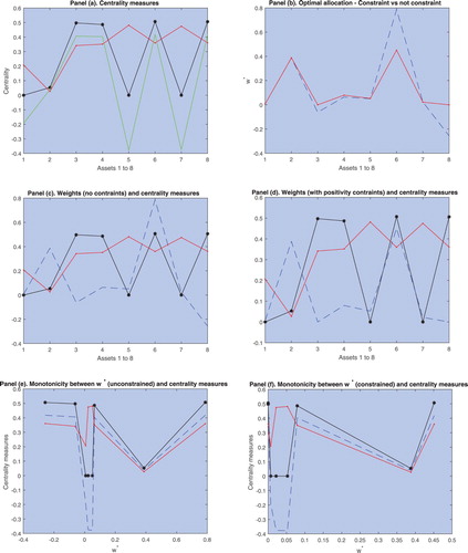
At the asset level, we find that the financial indexes (Dow Jones Industrial Average, Nasdaq 100 Index, S$\mathrm{\&}$P 500 Index and Willshire 5000 Price Index) exhibit large positive centrality measures, however, the CBOE volatility indexes and the exchange rate have values close to zero. This finding is mainly due to the large positive correlations (around 0.9) between the financial indexes. However, the volatility indexes and the exchange rate do not exhibit such correlations. More specifically, Table 2 shows that the sample correlation between the volatility indexes and the rest of assets in the portfolio is negative and around $-0.7$. These values explain the large negative centrality measures for the volatility indexes reported in figures 4 and 5.¹ The presence of a negative correlation between the volatility indexes, in particular the VIX index, and the conventional financial indexes is because the volatility assets are proxies for financial distress and uncertainty in financial markets. Thus, large values of these indexes are corresponded by negative returns of conventional financial indexes. In contrast, the different volatility indexes are positively cross-correlated with a correlation of 0.424 between the Russell 2000 Volatility index and the Gold ETF Volatility index, a correlation of 0.415 between the VIX and the Gold ETF Volatility index, and a correlation of 0.903 between the VIX and the Russell 2000 Volatility index. However, these correlations are not sufficient to make these assets positively central. Finally, the U.S./Euro exchange rate is uncorrelated to the rest of assets in the portfolio and the associated centrality measures are both close to zero, see figures 4 and 5.

Figure 4. CCC model with constrained weights. The black solid line denotes the positive centrality measure (10(10) $v_i^p={\overline{\lambda }}_1^{-1}\sum _{j=1}^n{\mathrm{\Lambda }}_{1,ij}{v}_j^p,$(10) ) and the red dashed line the negative centrality measure (11(11) $v_i^n={\overline{\lambda }}_2^{-1}\sum _{j=1}^n{\mathrm{\Lambda }}_{2,ij}{v}_j^n,$(11) ). The blue line denotes the dynamic optimal portfolio allocation over the evaluation period January 2011 to May 2020.

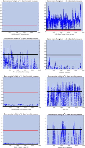
Figure 5. DCC model with constrained weights. The black solid line denotes the positive centrality measure (10(10) $v_i^p={\overline{\lambda }}_1^{-1}\sum _{j=1}^n{\mathrm{\Lambda }}_{1,ij}{v}_j^p,$(10) ) and the red dashed line the negative centrality measure (11(11) $v_i^n={\overline{\lambda }}_2^{-1}\sum _{j=1}^n{\mathrm{\Lambda }}_{2,ij}{v}_j^n,$(11) ). The blue line denotes the dynamic optimal portfolio allocation over the evaluation period January 2011 to May 2020.

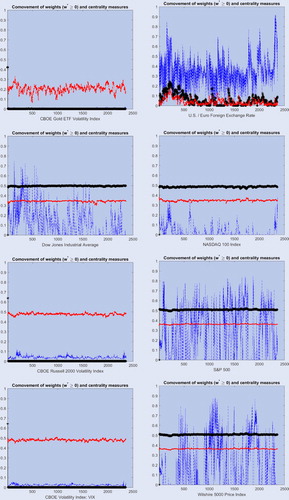
Table 2. Covariance and correlation matrix. January 2011 to May 2020.

Sample covariance matrix
Variable	Gold ETF Vol	U.S./Euro	DJIA	Nasdaq	Russell 2000 Vol	S$\mathrm{\&}$P 500	VIX	Willshire 5000
Gold ETF Vol	30.737
U.S./Euro	−0.207	0.579
DJIA	−1.924	0.064	1.207
Nasdaq	−2.081	0.056	1.202	1.524
Russell 2000 Vol	14.694	−0.255	−4.953	−5.754	39.122
S$\mathrm{\&}$P 500	−2.016	0.069	1.179	1.271	−5.214	1.206
VIX	18.357	−0.284	−6.242	−7.265	45.052	−6.573	63.637
Willshire 5000	−2.055	0.071	1.191	1.286	−5.334	1.222	−6.658	1.243
Sample correlation matrix
Variable	Gold ETF Vol	U.S./Euro	DJIA	Nasdaq	Russell 2000 Vol	S$\mathrm{\&}$P 500	VIX	Willshire 5000
Gold ETF Vol	1
U.S./Euro	−0.049	1
DJIA	−0.316	0.077	1
Nasdaq	−0.304	0.059	0.886	1
Russell 2000 Vol	0.424	−0.053	−0.721	−0.745	1
S$\mathrm{\&}$P 500	−0.331	0.083	0.977	0.937	−0.759	1
VIX	0.415	−0.046	−0.712	−0.737	0.903	−0.750	1
Willshire 5000	−0.332	0.084	0.972	0.934	−0.765	0.998	−0.748	1

The blue dashed line in figure 3(b) reports the weights obtained from expression (2(2) ${\mathbf{w}}^{\ast }=\frac{{\mathbf{\Sigma }}^{-1}\mathbf{1}}{{\mathbf{1}}^{\mathrm{\prime }}{\mathbf{\Sigma }}^{-1}\mathbf{1}}.$(2) ) and the red solid line reports the weights under short-selling restrictions ($\mathbf{w}\ge 0$). The only significant differences across portfolio allocations is between assets 6 (S$\mathrm{\&}$P 500 Index) and asset 8 (Willshire 5000 Price Index). The possibility of taking short positions in the first portfolio implies that it is optimal to obtain a larger positive position on the S$\mathrm{\&}$P 500 Index that is compensated by a negative position on the Willshire 5000 Price Index. Panels (c) and (d) report the centrality measures along with the unrestricted and restricted portfolio weights, respectively. No clear pattern emerges between the centrality measures and the optimal portfolio allocations. We observe large values of positive centrality accompanied by large allocations on the asset (asset 6) and similar values of positive centrality accompanied by small allocations on the asset (asset 8). Similar results are found for the relationship between negative centrality and the portfolio weights. These results are consistent with theorem 1 that shows that, in general, there does not exist a monotonic relationship between asset centrality and the optimal portfolio allocation. This result is at odds with the findings in Peralta and Zareei (2016) and Pozzi et al. (2013) that obtain a negative relationship between the optimal portfolio allocation and asset centrality.

To obtain more clarity on this relationship we rank the assets in terms of the portfolio weight from smallest to largest and report in Panels (e) and (f) of figure 3 the corresponding centrality measures associated to the weights. The existence of a monotonic relationship would emerge clearly in this graph in case it would exist, however, both graphs are rather inconclusive and do not show any clear pattern. Interestingly, we do observe clear comovements between the positive and negative centrality measures in both panels. The centrality measures move together up and down as the portfolio weights increase along the x axis. These findings provide further insights into the theoretical result in lemma 2 that derives the expression for the marginal rate of substitution between both centrality measures. In this example, the marginal rate of substitution is positive, that is, both measures move together up or down as the allocation to the portfolio varies. In Panel (e), both centrality measures decrease up to values of $w^{\ast }$ slightly greater than zero, then both measures increase and decrease again up to $w^{\ast }=0.4$. Finally, both centrality measures increase for values of the portfolio weight up to $w^{\ast }=0.8$. Similar results are found for Panel (f). In this case the optimal allocation of assets to the portfolio starts at $w^{\ast }=0$.

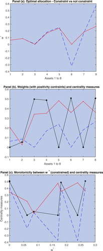
The above results show that the idiosyncratic variance of the volatility indexes plays an important role on the optimal portfolio allocation problem. The standard deviation of these fear indexes is several times higher than for the financial indexes and the U.S./Euro exchange rate. This means that the optimal allocation to these assets is close to zero regardless the covariance terms and centrality measures associated to these indexes. To abstract from these effects we study the portfolio allocation problem when the covariance matrix $\mathbf{\Sigma }$ is replaced by the correlation matrix $\mathbf{\Omega }$. In this scenario we assume that all assets have unit variance and the covariance is equal to the correlation. The centrality measures are the same of the previous case (Panel (a) of figure 3), however, the optimal asset allocation is more balanced across assets in the portfolio as Panel (a) of figure 6 illustrates. The short-selling constraint only affects the allocations to the S$\mathrm{\&}$P 500 and Willshire Indexes. Panels (b) and (c) of figure 6 compare the optimal weight allocation with the centrality measures. The results are similar to the previous exercise. We do not obtain a monotonic relationship between the portfolio weights and the centrality measures. This can be seen from comparing the allocations to assets 6 and 8 despite the fact that both assets have the same positive eigenvector centrality measure. Finally, Panel (c) of figure 6 ranks the assets on the portfolio weight and reports the centrality measures associated to each value of $w_i^{\ast }$. This graph confirms the absence of a monotonic relationship between the optimal weights and the centrality measures. The standard centrality measure (9(9) $v_i={\overline{\omega }}^{-1}\sum _{j=1}^n{\mathrm{\Omega }}_{ij}{v}_j,$(9) ) comoves with the positive centrality measure (10(10) $v_i^p={\overline{\lambda }}_1^{-1}\sum _{j=1}^n{\mathrm{\Lambda }}_{1,ij}{v}_j^p,$(10) ) defined herein but not with the negative centrality measure in (11(11) $v_i^n={\overline{\lambda }}_2^{-1}\sum _{j=1}^n{\mathrm{\Lambda }}_{2,ij}{v}_j^n,$(11) ).

Figure 6. Static analysis of centrality measures and portfolio weights. Panel (a): the red line denotes the constrained portfolio and the blue dashed line the unconstrained portfolio. Panel (b): the black solid line denotes the positive centrality measure (10(10) $v_i^p={\overline{\lambda }}_1^{-1}\sum _{j=1}^n{\mathrm{\Lambda }}_{1,ij}{v}_j^p,$(10) ) and the red dashed line the negative centrality measure (11(11) $v_i^n={\overline{\lambda }}_2^{-1}\sum _{j=1}^n{\mathrm{\Lambda }}_{2,ij}{v}_j^n,$(11) ). The blue dashed line denotes the optimal portfolio allocation for each asset. Panel (c): the black solid line denotes the positive centrality measure (10(10) $v_i^p={\overline{\lambda }}_1^{-1}\sum _{j=1}^n{\mathrm{\Lambda }}_{1,ij}{v}_j^p,$(10) ) and the red dashed line the negative centrality measure (11(11) $v_i^n={\overline{\lambda }}_2^{-1}\sum _{j=1}^n{\mathrm{\Lambda }}_{2,ij}{v}_j^n,$(11) ). The blue dashed line denotes the centrality measure (9(9) $v_i={\overline{\omega }}^{-1}\sum _{j=1}^n{\mathrm{\Omega }}_{ij}{v}_j,$(9) ).

3.2. Dynamic optimal portfolio allocation

In this section, we explore the centrality of assets in a dynamic framework. To do this, we consider two stylized models, the CCC model introduced by Bollerslev (1990) and the DCC model introduced by Engle (2002).

The conditional volatility process is denoted by the $n\times n$ matrix ${\mathbf{\Sigma }}_t$, with n the number of assets in the portfolio. The volatility process evolves according to the expression ${\mathbf{\Sigma }}_t={\mathbf{\Delta }}_t{\mathbf{\Omega }}_t{\mathbf{\Delta }}_t$, with ${\mathbf{\Delta }}_t$ a diagonal matrix with main diagonal elements given by the conditional variance ${\sigma }_{i,t}^2$ of asset i. The matrix ${\mathbf{\Omega }}_t$ denotes the conditional correlation matrix with elements given by ${\rho }_{ij,t}$. In the CCC model specification, the correlation matrix is constant over time such that ${\mathbf{\Sigma }}_t={\mathbf{\Delta }}_t\mathbf{\Omega }{\mathbf{\Delta }}_t$, and the diagonal elements of ${\mathbf{\Delta }}_t$ are usually modelled as univariate GARCH-type processes. In the DCC model, both variance and correlation matrices are time varying with elements that follow a GARCH(1,1)-type process. For example, the dynamic correlation matrix is defined as (14) ${\mathbf{\Omega }}_t=(1-{\alpha }_1-{\alpha }_2){\mathbf{\Omega }}_0+{\alpha }_1{\epsilon }_{t-1}{\epsilon }_{t-1}^{\mathrm{\prime }}+{\alpha }_2{\mathbf{\Omega }}_{t-1},$(14) with ${\alpha }_1$ and ${\alpha }_2$ the parameters of the model, ${\mathbf{\Omega }}_0=E\left[{\epsilon }_{t-1}{\epsilon }_{t-1}^{\mathrm{\prime }}\right]$ the unconditional correlation matrix and ${\epsilon }_{t-1}$ a $n\times 1$ zero-mean vector denoting the error term of the multivariate return process ${\mathbf{r}}_t=[r_{1t},\dots ,r_{nt}{]}^{\mathrm{\prime }}$. For example, in the simplest case, ${\mathbf{r}}_t={\mathbf{\Sigma }}_t^{1/2}{\epsilon }_t$, with ${\mathbf{\Sigma }}_t$ the conditional covariance matrix. More refined versions of the DCC model can be found in Aielli (2013) and Engle et al. (2019) for large-dimensional matrices.

In what follows, we describe the results of the dynamic minimum variance portfolio allocation exercise.

3.2.1. CCC model

In this exercise, we fit an AR(1)-GARCH(1,1) process for the univariate conditional volatility process for each of the eight assets in the portfolio and assume, by construction, that the conditional correlation matrix ${\mathbf{\Omega }}_t$ is constant over the evaluation period (January 2011 to May 2020). The top panel of table 3 reports the parameter estimates of $\mathbf{\Omega }$. The estimates of the univariate AR(1)-GARCH(1,1) process for each asset in the portfolio are not reported but are available from the author upon request.

Table 3. CCC and DCC correlation matrices. January 2011 to May 2020.

CCC correlation matrix
Variable	Gold ETF Vol	U.S./Euro	DJIA	Nasdaq	Russell 2000 Vol	S$\mathrm{\&}$P 500	VIX	Willshire 5000
Gold ETF Vol	1
U.S./Euro	−0.056	1
DJIA	−0.346	0.080	1
Nasdaq	−0.321	0.056	0.847	1
Russell 2000 Vol	0.432	−0.046	−0.766	−0.757	1
S$\mathrm{\&}$P 500	−0.362	0.080	0.963	0.922	−0.809	1
VIX	0.425	−0.047	−0.801	−0.778	0.899	−0.838	1
Willshire 5000	−0.363	0.079	0.956	0.920	−0.820	0.997	−0.837	1
DCC correlation matrix
Variable	Gold ETF Vol	U.S./Euro	DJIA	Nasdaq	Russell 2000 Vol	S$\mathrm{\&}$P 500	VIX	Willshire 5000
Gold ETF Vol	1
U.S./Euro	−0.062	1
DJIA	−0.317	0.107	1
Nasdaq	−0.286	0.079	0.847	1
Russell 2000 Vol	0.412	−0.074	−0.766	−0.750	1
S$\mathrm{\&}$P 500	−0.331	0.109	0.964	0.920	−0.808	1
VIX	0.402	−0.073	−0.796	−0.764	0.902	−0.830	1
Willshire 5000	−0.332	0.107	0.957	0.918	−0.818	0.997	−0.830	1
${\lambda }_1$	0.020${}^{\ast \ast \ast }$
${\lambda }_2$	0.945${}^{\ast \ast \ast }$

The optimal portfolio weights allocated to each asset in the portfolio presented above are obtained from applying expression (2(2) ${\mathbf{w}}^{\ast }=\frac{{\mathbf{\Sigma }}^{-1}\mathbf{1}}{{\mathbf{1}}^{\mathrm{\prime }}{\mathbf{\Sigma }}^{-1}\mathbf{1}}.$(2) ) to the one-period ahead dynamic covariance matrix ${\mathbf{\Sigma }}_t$ estimated each period. Our optimization exercise is done in-sample, that is, we use the full sample to estimate the model parameters and reconstruct the conditional variance process over the whole evaluation period by using one-period-ahead forecasts produced by the multivariate CCC model. In each period, we collect the predicted covariance process ${\hat{\mathbf{\Sigma }}}_t$ and apply the procedure developed above. That is, we obtain the estimated correlation matrix ${\hat{\mathbf{\Omega }}}_t$ as ${\hat{\mathbf{\Omega }}}_t={\hat{\mathbf{\Delta }}}_t^{-1}{\hat{\mathbf{\Sigma }}}_t^{-1}{\hat{\mathbf{\Delta }}}_t^{-1}$ and obtain the dynamic adjacency matrix ${\hat{\mathbf{\Lambda }}}_t$ as ${\hat{\mathbf{\Lambda }}}_t={\hat{\mathbf{\Omega }}}_t-{\mathbf{I}}_n$. From this matrix, we obtain ${\hat{\mathbf{\Lambda }}}_{1t}$ and ${\hat{\mathbf{\Lambda }}}_{2t}$ as ${\hat{\mathbf{\Lambda }}}_{1t}={\hat{\mathbf{\Lambda }}}_t\otimes \mathbf{1}({\hat{\mathbf{\Lambda }}}_t>0)$. Similarly, we obtain ${\hat{\mathbf{\Lambda }}}_{2t}=-{\hat{\mathbf{\Lambda }}}_t\otimes \mathbf{1}({\hat{\mathbf{\Lambda }}}_t<0)$. Both matrices are symmetric and accommodate, in turn, an spectral decomposition such that we obtain the eigenvalues and corresponding eigenvectors that are collected in matrices ${\hat{\mathbf{U}}}_1$ and ${\hat{\mathbf{U}}}_2$. The eigenvector centrality measures ${\mathbf{v}}^p$ and ${\mathbf{v}}^n$ are obtained from these matrices of eigenvectors using expressions (10(10) $v_i^p={\overline{\lambda }}_1^{-1}\sum _{j=1}^n{\mathrm{\Lambda }}_{1,ij}{v}_j^p,$(10) ) and (11(11) $v_i^n={\overline{\lambda }}_2^{-1}\sum _{j=1}^n{\mathrm{\Lambda }}_{2,ij}{v}_j^n,$(11) ).

Figure 4 reports the optimal weight allocation and associated centrality measures for the eight assets in the portfolio over the evaluation period. Each panel considers a different asset and reports the centrality measures $v_i^p$ and $v_i^n$, and the optimal portfolio allocation $w_{it}^{\ast }$ over the evaluation period. For space constraints, we only report the portfolio allocation under short-selling constraints, however, as shown in figures 3 and 6, the results when the short-selling constraints are relaxed are very similar but with the optimal weights including negative values. The results for this case are available from the author upon request.

The estimates of the centrality measures are plotted by a black line ($\ast -$) for positive centrality ${\mathbf{v}}^p$ and a red line ($\cdot -$) for negative centrality ${\mathbf{v}}^n$. These quantities are estimated each period and, in principle, could vary over time, however, they remain constant over the evaluation period due to the choice of the CCC model specification that assumes a constant correlation matrix. The dynamic allocation to the volatility indexes (Gold ETF, Russell 2000 and VIX) is very small over the evaluation period. The corresponding positive centrality statistic is also very small but the negative eigenvector centrality measure is large. These results show that these assets are not positively correlated to any other asset in the portfolio, however, they are negatively correlated to some of the other assets in the portfolio. This was the primary reason to include them in the investment portfolio. These results also contradict the current view that asset centrality has a negative effect on the asset allocation. In this example, we see that positive asset centrality is very low and the associated asset allocation is almost zero. We should also note that in this example our positive centrality measure is positively correlated to the centrality measure proposed in the literature in (9(9) $v_i={\overline{\omega }}^{-1}\sum _{j=1}^n{\mathrm{\Omega }}_{ij}{v}_j,$(9) ).

The contribution of the U.S./Euro exchange rate to the portfolio is sizeable and stable over time despite the fact that the centrality measures corresponding to this asset are very small. In contrast, the allocation to the Nasdaq Index is small but the centrality statistics are large and of similar magnitude to the other financial indexes in the portfolio. The difference in portfolio allocation between these assets is driven by differences in the idiosyncratic risk given by the asset variance. The allocations to the Dow Jones and Willshire 5000 Price Index are more volatile than the allocation to the S$\mathrm{\&}$P 500 Index.

Overall, the message that emerges from this empirical analysis is that the financial indexes are positively correlated among each other but negatively correlated to the volatility indexes. This pattern of correlations produces the positive and negative centrality measures that we observe, that are not monotonically related to the optimal asset allocation.

3.2.2. DCC model

The previous analysis is extended to consider a dynamic correlation matrix ${\mathbf{\Omega }}_t$. The bottom panel of table 3 reports the parameter estimates of the unconditional correlation matrix ${\mathbf{\Omega }}_0$ and the estimates of ${\alpha }_1$ and ${\alpha }_2$ that drive the dynamic conditional correlation structure. Both parameters are statistically significant and satisfy the conditions to imply that the conditional correlation processes are weakly stationary.

In this case the adjacency matrix ${\mathbf{\Lambda }}_t$ is allowed to vary over time as well as the conditional variance processes. Therefore, the centrality measures are dynamic. Despite the added flexibility, the results in figure 5 are similar to the CCC case. The positive centrality measures are very stable over time for all the assets in the portfolio. The negative centrality measures exhibit more variation, in particular, for the Gold ETF volatility index and the U.S./Euro exchange rate. The latter asset provides the most interesting insights in terms of asset centrality. Both centrality measures move together up and down over the evaluation period. The exchange rate seems to take a more central role in the portfolio during the first years of the evaluation period that coincides with a spike on the allocation to the asset in the portfolio. The asset centrality decays after 2014 and stays low for the remaining of the evaluation period.

4. Conclusion

This paper studies the relationship between the optimal allocation of assets in a portfolio and the corresponding asset centrality statistic. First, we show that the standard definition of eigenvector centrality found in the literature, see Bonacich (1972), is misleading when the adjacency matrix in a network can take negative values. In this case, the centrality measure can take negative values, which does not have a natural interpretation. More importantly, the centrality of assets can cancel out for assets highly correlated (positively correlated) to the rest of assets in the portfolio. To correct for this, we have introduced the concept of positive and negative eigenvector centrality. This extension of Bonacich's (1972) eigenvector centrality fits naturally in a global minimum variance portfolio allocation problem in which the adjacency matrix is characterized by the correlation matrix between asset returns.

For portfolios with short-selling constraints we prove that portfolio risk is strictly increasing on positive asset centrality. This result does not imply, however, the presence of a negative relationship between the magnitude of the optimal asset allocation to the portfolio and the centrality measure. In fact, we prove the absence of a monotonic relationship between positive asset centrality and the optimal portfolio allocation. Similarly, we find a strictly decreasing relationship between negative asset centrality and portfolio risk that is not reflected on a positive relationship between asset centrality and the optimal portfolio allocation. These results contradict recent results on the literature on financial networks claiming that asset centrality and the optimal portfolio allocation are negatively related. As a byproduct, we also find that the marginal rate of substitution between positive and negative asset centrality is positive. Both centrality measures tend to move together in the same direction to preserve the optimal allocation of an asset in a portfolio.

More generally, under the absence of short-selling constraints we do not find a monotonic relationship between portfolio risk and asset centrality or between the optimal asset allocation and asset centrality. These results are confirmed in an empirical application to a mix of assets with positive and negative cross-correlations.

Disclosure statement

No potential conflict of interest was reported by the author.

Additional information

Funding

This work was supported by project PID2019-104326GB-I00 from Ministerio de Ciencia e Innovación and from Fundación Agencia Aragonesa para la Investigación y el Desarrollo (ARAID).

Notes

1 Table 2 uses nonparametric estimators based on the naive empirical distribution function for the static covariance matrix. These estimators provide consistent estimates of the idiosyncratic variances and covariances under stationarity of the vector of log returns and when the time dimension T increases to infinity. An additional restriction is that the number of assets in the portfolio is fixed or increases to infinity but a lower rate than T, that is, $n/T\to 0$, with $n,T\to \mathrm{\infty }$. In our exercise, n = 8 is small compared to T = 2400 implying that the estimates of the covariance matrix are consistent. When the number of assets increases with T, Ledoit and Wolf 2003 and Engle et al. 2019 propose shrinkage methods to estimate the covariance matrix in static and dynamic settings.

Appendix. Mathematical appendix

Proof

Proof of Proposition 1

Let $\mathbf{\Theta }=c_1{\mathbf{I}}_n+c_2\mathbf{\Lambda }$ be a location-scale transformation of the adjacency matrix $\mathbf{\Lambda }$ characterized by the constants $c_1\in \mathbb{R}$ and $c_2>0$; and let $(v_i^p,v_i^n)$ be the positive and negative eigenvector centrality measures associated to $\mathbf{\Lambda }$. First, we show that the centrality measures of ${\mathbf{\Theta }}_0=c_2\mathbf{\Lambda }$ are the same of the adjacency matrix $\mathbf{\Lambda }$. To show this, we decompose the matrix as ${\mathbf{\Theta }}_0={\mathbf{\Theta }}_{01}+{\mathbf{\Theta }}_{02}$, with ${\mathbf{\Theta }}_{01}={\mathbf{\Theta }}_0\mathbf{1}({\mathbf{\Theta }}_0>0)$ and ${\mathbf{\Theta }}_{02}=-{\mathbf{\Theta }}_0\mathbf{1}({\mathbf{\Theta }}_0<0)$. The positive centrality measure of ${\mathbf{\Theta }}_0$, denoted as $z_{0i}^p$, is defined using condition (10(10) $v_i^p={\overline{\lambda }}_1^{-1}\sum _{j=1}^n{\mathrm{\Lambda }}_{1,ij}{v}_j^p,$(10) ) as (A1) $z_{0i}^p={\overline{\theta }}_{01}^{-1}\sum _{j=1}^n{\mathrm{\Theta }}_{01,ij}{z}_{0j}^p,$(A1) with ${\overline{\theta }}_{01}$ the maximum eigenvalue of ${\mathbf{\Theta }}_{01}$ and ${\mathrm{\Theta }}_{01,ij}$ the elements of the matrix ${\mathbf{\Theta }}_{01}$. Now, we note that ${\overline{\theta }}_{01}=c_2{\overline{\lambda }}_1$, with ${\overline{\lambda }}_1$ the maximum eigenvalue of ${\mathbf{\Lambda }}_1$, and ${\mathbf{\Theta }}_{01}=c_2{\mathbf{\Lambda }}_1$. Then, condition (A1(A1) $z_{0i}^p={\overline{\theta }}_{01}^{-1}\sum _{j=1}^n{\mathrm{\Theta }}_{01,ij}{z}_{0j}^p,$(A1) ) is equivalent to $z_{0i}^p={\overline{\lambda }}_1^{-1}\sum _{j=1}^n{\mathrm{\Lambda }}_{1,ij}{z}_{0j}^p.$ Therefore, from expression (10(10) $v_i^p={\overline{\lambda }}_1^{-1}\sum _{j=1}^n{\mathrm{\Lambda }}_{1,ij}{v}_j^p,$(10) ), we have ${\mathbf{z}}_0^p={\mathbf{v}}^p$. Using the same arguments for matrices ${\mathbf{\Theta }}_{02}$ and ${\mathbf{\Lambda }}_2$, it can be easily shown that ${\mathbf{z}}_0^n={\mathbf{v}}^n$.

In a second step, we prove that the centrality measures of $\mathbf{\Theta }=c_1{\mathbf{I}}_n+{\mathbf{\Theta }}_0$ are the same of the matrix ${\mathbf{\Theta }}_0$. Let $z_i^p$ denote the positive eigenvector centrality measure of $\mathbf{\Theta }$. Then, (A2) $z_i^p={\overline{\theta }}^{-1}\sum _{j=1}^n{\mathrm{\Theta }}_{ij}{z}_j^p,$(A2) with $\overline{\theta }$ the maximum eigenvalue of $\mathbf{\Theta }$ and ${\mathrm{\Theta }}_{ij}$ the elements of the matrix. To show the result, we note that the eigenvalues of $\mathbf{\Theta }$ satisfy that ${\theta }_k=c_1+{\theta }_{01,k}$, with ${\theta }_k$ and ${\theta }_{01,k}$ the eigenvalues of $\mathbf{\Theta }$ and ${\mathbf{\Theta }}_0$. In particular, we have $\overline{\theta }=c_1+{\overline{\theta }}_{01}$. Then, replacing in (A2(A2) $z_i^p={\overline{\theta }}^{-1}\sum _{j=1}^n{\mathrm{\Theta }}_{ij}{z}_j^p,$(A2) ), we obtain $(c_1+{\overline{\theta }}_{01})z_i^p=c_1{z}_i^p+\sum _{\begin{array}{c}j\ne i\\ j=1\end{array}}^n{\mathrm{\Theta }}_{ij}{z}_j^p.$ Therefore, ${\overline{\theta }}_{01}{z}_i^p=\sum _{\begin{array}{c}j\ne i\\ j=1\end{array}}^n{\mathrm{\Theta }}_{ij}{z}_j^p$. Finally, we note that this condition is equivalent to ${\overline{\theta }}_{01}{z}_i^p=\sum _{\begin{array}{c}j\ne i\\ j=1\end{array}}^n{\mathrm{\Theta }}_{0,ij}{z}_j^p,$ with ${\mathrm{\Theta }}_{0,ij}$ the elements of the matrix ${\mathbf{\Theta }}_0$, and implying that ${\mathbf{z}}^p={\mathbf{z}}_0^p$. Using similar arguments, it is straightforward to obtain that ${\mathbf{z}}^n={\mathbf{z}}_0^n$.

Proof

Proof of Proposition 2

To show this result note from expression (6(6) $Q(\mathbf{\Sigma },\mathbf{w})={\mathbf{w}}^{\mathrm{\prime }}\mathbf{\Sigma }\mathbf{w}={\tilde{\mathbf{w}}}^{\mathrm{\prime }}\mathbf{\Omega }\tilde{\mathbf{w}}={\tilde{\mathbf{w}}}^{\mathrm{\prime }}\mathbf{\Lambda }\tilde{\mathbf{w}}+{\tilde{\mathbf{w}}}^{\mathrm{\prime }}\tilde{\mathbf{w}},$(6) ) that ${\tilde{\mathbf{w}}}^{\mathrm{\prime }}\mathbf{\Lambda }\tilde{\mathbf{w}}={\tilde{\mathbf{w}}}^{\mathrm{\prime }}[{\mathbf{\Lambda }}_1-{\mathbf{\Lambda }}_2]\tilde{\mathbf{w}}={\tilde{\mathbf{w}}}^{\mathrm{\prime }}{\mathbf{U}}_1{\mathbf{D}}_{{\lambda }_1}{\mathbf{U}}_1^{\mathrm{\prime }}\tilde{\mathbf{w}}-{\tilde{\mathbf{w}}}^{\mathrm{\prime }}{\mathbf{U}}_2{\mathbf{D}}_{{\lambda }_2}{\mathbf{U}}_2^{\mathrm{\prime }}\tilde{\mathbf{w}}.$ The matrix ${\mathbf{U}}_1$ contains the eigenvectors of ${\mathbf{\Lambda }}_1$ and ${\mathbf{\Omega }}_1$ such that the positive eigenvector centrality measure $v_i^p$ is the eigenvector associated to the largest eigenvalue of these matrices. Similarly, the negative eigenvector centrality measure $v_i^n$ is the eigenvector from the matrix ${\mathbf{U}}_2$ associated to the largest eigenvalue of the matrix ${\mathbf{\Lambda }}_{\mathbf{2}}={\mathbf{\Omega }}_2$.

The quadratic form capturing the network dependencies can be expressed as (A3) ${\tilde{\mathbf{w}}}^{\mathrm{\prime }}\mathbf{\Lambda }\tilde{\mathbf{w}}=\sum _{i=1}^n{\lambda }_{1i}{\left(\sum _{j=1}^n{\tilde{\mathrm{w}}}_j{u}_{1,ji}\right)}^2-\sum _{i=1}^n{\lambda }_{2i}{\left(\sum _{j=1}^n{\tilde{\mathrm{w}}}_j{u}_{2,ji}\right)}^2,$(A3) with $u_{1,ij}$ and $u_{2,ij}$ the elements of the matrices ${\mathbf{U}}_1$ and ${\mathbf{U}}_2$, respectively. This expression can be written as a function of $v_i^p$ as (A4) $\begin{array}{rl}{\tilde{\mathbf{w}}}^{\mathrm{\prime }}\mathbf{\Lambda }\tilde{\mathbf{w}}& ={\overline{\lambda }}_1{\left(\sum _{j=1}^n{\tilde{\mathrm{w}}}_j{v}_j^p\right)}^2+\sum _{i=2}^n{\lambda }_{1i}{\left(\sum _{j=1}^n{\tilde{\mathrm{w}}}_j{u}_{1,ji}\right)}^2\\ & -\sum _{i=1}^n{\lambda }_{2i}{\left(\sum _{j=1}^n{\tilde{\mathrm{w}}}_j{u}_{2,ji}\right)}^2.\end{array}$(A4) The first derivative of the loss function associated to the adjacency matrix $\mathbf{\Lambda }$ with respect to the positive centrality measure $v_i^p$ is $\frac{\mathrm{\partial }{\tilde{\mathbf{w}}}^{\mathrm{\prime }}\mathbf{\Lambda }\tilde{\mathbf{w}}}{\mathrm{\partial }{v}_i^p}=\frac{\mathrm{\partial }{\overline{\lambda }}_1}{\mathrm{\partial }{v}_i^p}{\left(\sum _{j=1}^n{\tilde{\mathrm{w}}}_j{v}_j^p\right)}^2+2{\overline{\lambda }}_1{\tilde{\mathrm{w}}}_i\left(\sum _{j=1}^n{\tilde{\mathrm{w}}}_j{v}_j^p\right).$ By construction, ${\lambda }_{1k}=\sum _{i=1}^n\sum _{\begin{array}{c}j\ne i\\ j=1\end{array}}^n{u}_{1,ik}{u}_{1,jk}{\mathrm{\Lambda }}_{1,ij}$. Then, for the largest eigenvalue we obtain ${\overline{\lambda }}_1=\sum _{i=1}^n\sum _{\begin{array}{c}j\ne i\\ j=1\end{array}}^n{v}_i^p{v}_j^p{\mathrm{\Lambda }}_{1,ij}$, where $v_i^p=u_{1,i1}$ such that $\frac{\mathrm{\partial }{\overline{\lambda }}_1}{\mathrm{\partial }{v}_i^p}=\sum _{\begin{array}{c}j\ne i\\ j=1\end{array}}^n{\mathrm{\Lambda }}_{1,ij}{v}_j^p$. The definition of eigenvector centrality (10(10) $v_i^p={\overline{\lambda }}_1^{-1}\sum _{j=1}^n{\mathrm{\Lambda }}_{1,ij}{v}_j^p,$(10) ) implies that $\sum _{\begin{array}{c}j\ne i\\ j=1\end{array}}^n{\mathrm{\Lambda }}_{1,ij}{v}_j^p={\overline{\lambda }}_1{v}_i^p$ such that $\frac{\mathrm{\partial }{\overline{\lambda }}_1}{\mathrm{\partial }{v}_i^p}={\overline{\lambda }}_1{v}_i^p$. Following similar arguments we obtain $\frac{\mathrm{\partial }{\lambda }_{1k}}{\mathrm{\partial }{v}_i^p}=0$, for $k=2,\dots ,n$. Then, the above expression reads as $\frac{\mathrm{\partial }{\tilde{\mathbf{w}}}^{\mathrm{\prime }}\mathbf{\Lambda }\tilde{\mathbf{w}}}{\mathrm{\partial }{v}_i^p}={\overline{\lambda }}_1{v}_i^p{\left(\sum _{j=1}^n{\tilde{\mathrm{w}}}_j{v}_j^p\right)}^2+2{\overline{\lambda }}_1{\tilde{\mathrm{w}}}_i\left(\sum _{j=1}^n{\tilde{\mathrm{w}}}_j{v}_j^p\right).$ In general, this expression can be positive or negative. Note that the maximum eigenvalue ${\overline{\lambda }}_1$ and the centrality measures $v_i^p$, for $i=1,\dots ,n$ are both positive. Then, for investment portfolios constructed under short-selling constraints, it follows that $\tilde{\mathbf{w}}>\mathbf{0}$, such that there is a positive monotonic relationship between the loss function ${\tilde{\mathbf{w}}}^{\mathrm{\prime }}\mathbf{\Lambda }\tilde{\mathbf{w}}$ and positive asset centrality.

Proof

Proof of Proposition 3

To show this result we follow closely the proof of Proposition 2. The quadratic form (A3(A3) ${\tilde{\mathbf{w}}}^{\mathrm{\prime }}\mathbf{\Lambda }\tilde{\mathbf{w}}=\sum _{i=1}^n{\lambda }_{1i}{\left(\sum _{j=1}^n{\tilde{\mathrm{w}}}_j{u}_{1,ji}\right)}^2-\sum _{i=1}^n{\lambda }_{2i}{\left(\sum _{j=1}^n{\tilde{\mathrm{w}}}_j{u}_{2,ji}\right)}^2,$(A3) ) capturing the network dependencies can be written as a function of $v_i^n$ as (A5) $\begin{array}{rl}{\tilde{\mathbf{w}}}^{\mathrm{\prime }}\mathbf{\Lambda }\tilde{\mathbf{w}}& =\sum _{i=1}^n{\lambda }_{1i}{\left(\sum _{j=1}^n{\tilde{\mathrm{w}}}_j{u}_{1,ji}\right)}^2-{\overline{\lambda }}_2{\left(\sum _{j=1}^n{\tilde{\mathrm{w}}}_j{v}_j^n\right)}^2\\ & -\sum _{i=1}^n{\lambda }_{2i}{\left(\sum _{j=1}^n{\tilde{\mathrm{w}}}_j{u}_{2,ji}\right)}^2.\end{array}$(A5) The first derivative with respect to the negative centrality measure $v_i^n$ is $\frac{\mathrm{\partial }{\tilde{\mathbf{w}}}^{\mathrm{\prime }}\mathbf{\Lambda }\tilde{\mathbf{w}}}{\mathrm{\partial }{v}_i^n}=-\frac{\mathrm{\partial }{\overline{\lambda }}_2}{\mathrm{\partial }{v}_i^n}{\left(\sum _{j=1}^n{\tilde{\mathrm{w}}}_j{v}_j^n\right)}^2-2{\overline{\lambda }}_2{\tilde{\mathrm{w}}}_i\left(\sum _{j=1}^n{\tilde{\mathrm{w}}}_j{v}_j^n\right).$ By construction, ${\lambda }_{2k}=\sum _{i=1}^n\sum _{\begin{array}{c}j\ne i\\ j=1\end{array}}^n{u}_{2,ik}{u}_{2,jk}{\mathrm{\Lambda }}_{2,ij}$. Then, for the largest eigenvalue we obtain ${\overline{\lambda }}_2=\sum _{i=1}^n\sum _{\begin{array}{c}j\ne i\\ j=1\end{array}}^n{v}_i^n{v}_j^n{\mathrm{\Lambda }}_{2,ij}$, where $v_i^n=u_{2,i1}$ such that $\frac{\mathrm{\partial }{\overline{\lambda }}_2}{\mathrm{\partial }{v}_i^n}=\sum _{\begin{array}{c}j\ne i\\ j=1\end{array}}^n{\mathrm{\Lambda }}_{2,ij}{v}_j^n$. The definition of eigenvector centrality (11(11) $v_i^n={\overline{\lambda }}_2^{-1}\sum _{j=1}^n{\mathrm{\Lambda }}_{2,ij}{v}_j^n,$(11) ) implies that $\sum _{\begin{array}{c}j\ne i\\ j=1\end{array}}^n{\mathrm{\Lambda }}_{2,ij}{v}_j^n={\overline{\lambda }}_2{v}_i^n$ such that $\frac{\mathrm{\partial }{\overline{\lambda }}_2}{\mathrm{\partial }{v}_i^n}={\overline{\lambda }}_2{v}_i^n$. Following similar arguments, we obtain $\frac{\mathrm{\partial }{\lambda }_{2k}}{\mathrm{\partial }{v}_i^n}=0$ for $k=2,\dots ,n$. Then, the above expression reads as $\frac{\mathrm{\partial }{\tilde{\mathbf{w}}}^{\mathrm{\prime }}\mathbf{\Lambda }\tilde{\mathbf{w}}}{\mathrm{\partial }{v}_i^n}=-{\overline{\lambda }}_2{v}_i^n{\left(\sum _{j=1}^n{\tilde{\mathrm{w}}}_j{v}_j^n\right)}^2-2{\overline{\lambda }}_2{\tilde{\mathrm{w}}}_i\left(\sum _{j=1}^n{\tilde{\mathrm{w}}}_j{v}_j^n\right).$ In general, this expression can be positive or negative. Note that the maximum eigenvalue ${\overline{\lambda }}_2$ and the centrality measures $v_i^n$, for $i=1,\dots ,n$ are both positive. Then, for investment portfolios constructed under short-selling constraints, it follows that $\tilde{\mathbf{w}}>\mathbf{0}$, such that there is a negative monotonic relationship between the loss function ${\tilde{\mathbf{w}}}^{\mathrm{\prime }}\mathbf{\Lambda }\tilde{\mathbf{w}}$ and negative asset centrality.

Proof

Proof of Proposition 4

Expression (2(2) ${\mathbf{w}}^{\ast }=\frac{{\mathbf{\Sigma }}^{-1}\mathbf{1}}{{\mathbf{1}}^{\mathrm{\prime }}{\mathbf{\Sigma }}^{-1}\mathbf{1}}.$(2) ) shows that ${\mathbf{w}}^{\ast }=\frac{{\mathbf{\Sigma }}^{-1}\mathbf{1}}{{\mathbf{1}}^{\mathrm{\prime }}{\mathbf{\Sigma }}^{-1}\mathbf{1}}$, with $\mathbf{\Sigma }=\mathbf{\Delta }\mathbf{\Omega }\mathbf{\Delta }$. The inverse of the covariance matrix is ${\mathbf{\Sigma }}^{-1}={\mathbf{\Delta }}^{-1}{\mathbf{\Omega }}^{-1}{\mathbf{\Delta }}^{-1}$, with ${\mathbf{\Omega }}^{-1}=\mathbf{U}{\mathbf{D}}_{\omega }^{-1}{\mathbf{U}}^{\mathrm{\prime }}$. Then, ${\mathrm{w}}_i^{\ast }=\frac{\left[{\mathbf{\Delta }}^{-1}\mathbf{U}{]}_i{\mathbf{D}}_{\omega }^{-1}\right[{\mathbf{\Delta }}^{-1}\mathbf{U}{]}^{\mathrm{\prime }}\mathbf{1}}{{\mathbf{1}}^{\mathrm{\prime }}\left[{\mathbf{\Delta }}^{-1}\mathbf{U}\right]{\mathbf{D}}_{\omega }^{-1}[{\mathbf{\Delta }}^{-1}\mathbf{U}{]}^{\mathrm{\prime }}\mathbf{1}},$ with $[{\mathbf{\Delta }}^{-1}\mathbf{U}{]}_i$ denoting the row i of dimension $1\times n$ of the matrix ${\mathbf{\Delta }}^{-1}\mathbf{U}$. Applying matrix algebra, we obtain ${\mathrm{w}}_i^{\ast }=\frac{\sum _{k=1}^n\frac{u_{ik}}{{\omega }_k{\sigma }_i}\left(\sum _{j=1}^n\frac{1}{{\sigma }_j}{u}_{jk}\right)}{\sum _{k=1}^n\frac{1}{{\omega }_k}{\left(\sum _{j=1}^n\frac{1}{{\sigma }_j}{u}_{jk}\right)}^2},$ with the eigenvalues ${\omega }_k$ that can be expressed as a function of the centrality measures $v_i^p$ and $v_i^n$ as shown in expression (12(12) $\begin{array}{rl}{\omega }_k& =1+{\overline{\lambda }}_1{\left(\sum _{j=1}^n{u}_{jk}{v}_j^p\right)}^2-{\overline{\lambda }}_2{\left(\sum _{j=1}^n{u}_{jk}{v}_j^n\right)}^2\\ & +\sum _{i=2}^n\left[{\lambda }_{1i}{\left(\sum _{j=1}^n{u}_{jk}{u}_{1,ji}\right)}^2-{\lambda }_{2i}{\left(\sum _{j=1}^n{u}_{jk}{u}_{2,ji}\right)}^2\right].\end{array}$(12) ).

Proof

Proof of Theorem 1

We write expression (13(13) ${\mathrm{w}}_i^{\ast }=\frac{\sum _{k=1}^n{\tilde{\omega }}_k\frac{u_{ik}}{{\sigma }_i}\left(\sum _{j=1}^n\frac{1}{{\sigma }_j}{u}_{jk}\right)}{\sum _{k=1}^n{\tilde{\omega }}_k{\left(\sum _{j=1}^n\frac{1}{{\sigma }_j}{u}_{jk}\right)}^2},$(13) ) as ${\mathrm{w}}_i^{\ast }=\frac{\sum _{k=1}^n{\tilde{\omega }}_k\frac{u_{ik}}{{\sigma }_i}\left(\sum _{j=1}^n\frac{1}{{\sigma }_j}{u}_{jk}\right)}{\sum _{k=1}^n{\tilde{\omega }}_k(\sum _{j=1}^n\frac{1}{{\sigma }_j}{u}_{jk}{)}^2},\text{ with }{\tilde{\omega }}_k=\frac{1}{{\omega }_k}.$

To assess the relationship between asset centrality and the optimal portfolio allocation we study the first derivative of ${\mathrm{w}}_i^{\ast }$ with respect to $v_i^p$. This expression can be written as $\frac{\mathrm{\partial }{\mathrm{w}}_i^{\ast }}{\mathrm{\partial }{v}_i^p}=\frac{\begin{array}{c}\sum _{k=1}^n\frac{\mathrm{\partial }{\tilde{\omega }}_k}{\mathrm{\partial }{v}_i^p}\frac{u_{ik}}{{\sigma }_i}{a}_k\left(\sum _{s=1}^n{\tilde{\omega }}_s{a}_s^2\right)\\ -\sum _{k=1}^n{\tilde{\omega }}_k\frac{u_{ik}}{{\sigma }_i}{a}_k\left(\sum _{s=1}^n\frac{\mathrm{\partial }{\tilde{\omega }}_s}{\mathrm{\partial }{v}_i^p}{a}_s^2\right)\end{array}}{{\left(\sum _{k=1}^n{\tilde{\omega }}_k{a}_k^2\right)}^2},$ with $a_s=\sum _{j=1}^n\frac{1}{{\sigma }_j}{u}_{js}$. In what follows, we focus on the numerator of $\frac{\mathrm{\partial }{\mathrm{w}}_i^{\ast }}{\mathrm{\partial }{v}_i^p}$, that we denote as $\frac{\mathrm{\partial }{\mathrm{w}}_i^{\ast }}{\mathrm{\partial }{v}_i^p}{|}_{Num}$ and study the conditions that guarantee that this expression is positive or negative over the values of the centrality measure. Using simple algebra, the numerator of the above expression is $\begin{array}{rl}\frac{\mathrm{\partial }{\mathrm{w}}_i^{\ast }}{\mathrm{\partial }{v}_i^p}{|}_{Num}& =\sum _{k=1}^n\left(\frac{\mathrm{\partial }{\tilde{\omega }}_k}{\mathrm{\partial }{v}_i^p}-{\tilde{\omega }}_k\right)\frac{u_{ik}}{{\sigma }_i}{a}_k\left(\sum _{s=1}^n{\tilde{\omega }}_s{a}_s^2\right)\\ & -\sum _{k=1}^n{\tilde{\omega }}_k\frac{u_{ik}}{{\sigma }_i}{a}_k\left[\sum _{s=1}^n\frac{\mathrm{\partial }{\tilde{\omega }}_s}{\mathrm{\partial }{v}_i^p}{a}_s^2-\left(\sum _{s=1}^n{\tilde{\omega }}_s{a}_s^2\right)\right]\\ & =\sum _{k=1}^n\left(\frac{\mathrm{\partial }{\tilde{\omega }}_k}{\mathrm{\partial }{v}_i^p}-{\tilde{\omega }}_k\right)\frac{u_{ik}}{{\sigma }_i}{a}_k\left(\sum _{s=1}^n{\tilde{\omega }}_s{a}_s^2\right)\\ & -\sum _{k=1}^n{\tilde{\omega }}_k\frac{u_{ik}}{{\sigma }_i}{a}_k\left[\sum _{s=1}^n\left(\frac{\mathrm{\partial }{\tilde{\omega }}_s}{\mathrm{\partial }{v}_i^p}-{\tilde{\omega }}_s\right)a_s^2\right].\end{array}$ Furthermore, note that ${\tilde{\omega }}_k=\frac{1}{{\omega }_k}$ for $k=1,\dots ,n$. Then, from expression (12(12) $\begin{array}{rl}{\omega }_k& =1+{\overline{\lambda }}_1{\left(\sum _{j=1}^n{u}_{jk}{v}_j^p\right)}^2-{\overline{\lambda }}_2{\left(\sum _{j=1}^n{u}_{jk}{v}_j^n\right)}^2\\ & +\sum _{i=2}^n\left[{\lambda }_{1i}{\left(\sum _{j=1}^n{u}_{jk}{u}_{1,ji}\right)}^2-{\lambda }_{2i}{\left(\sum _{j=1}^n{u}_{jk}{u}_{2,ji}\right)}^2\right].\end{array}$(12) ), and noting that $\frac{\mathrm{\partial }{\overline{\lambda }}_1}{\mathrm{\partial }{v}_i^p}={\overline{\lambda }}_1{v}_i^p$, it follows that (A6) $\begin{array}{rl}\frac{\mathrm{\partial }{\tilde{\omega }}_k}{\mathrm{\partial }{v}_i^p}& =-\frac{\mathrm{\partial }{\omega }_k/\mathrm{\partial }{v}_i^p}{{\omega }_k^2}\\ & =-\frac{1}{{\omega }_k^2}\left[{\overline{\lambda }}_1{v}_i^p{\left(\sum _{j=1}^n{u}_{jk}{v}_j^p\right)}^2+2{\overline{\lambda }}_1{u}_{ik}\left(\sum _{j=1}^n{u}_{jk}{v}_j^p\right)\right],\end{array}$(A6) such that $\begin{array}{rl}& \frac{\mathrm{\partial }{\tilde{\omega }}_k}{\mathrm{\partial }{v}_i^p}-{\tilde{\omega }}_k\\ & =-\frac{1}{{\omega }_k^2}\left[{\overline{\lambda }}_1{v}_i^p{\left(\sum _{j=1}^n{u}_{jk}{v}_j^p\right)}^2+2{\overline{\lambda }}_1{u}_{ik}\left(\sum _{j=1}^n{u}_{jk}{v}_j^p\right)+{\omega }_k\right].\end{array}$ Therefore, the above expression can take positive or negative values showing that the derivative of the weight function ${\mathrm{w}}_i^{\ast }$ is not monotonic with respect to the eigenvector centrality measure $v_i^p$ unless for special configurations of the matrix $\mathbf{U}$ and the idiosyncratic variances ${\sigma }_i$ for $i=1,\dots ,n$.

Similarly, we can repeat the exercise for the negative centrality measures. In this case, it follows that (A7) $\begin{array}{rl}\frac{\mathrm{\partial }{\tilde{\omega }}_k}{\mathrm{\partial }{v}_i^n}& =-\frac{\mathrm{\partial }{\overline{\omega }}_k/\mathrm{\partial }{v}_i^n}{{\omega }_k^2}\\ & =\frac{1}{{\omega }_k^2}\left[{\overline{\lambda }}_2{v}_i^n{\left(\sum _{j=1}^n{u}_{jk}{v}_j^n\right)}^2+2{\overline{\lambda }}_2{u}_{ik}\left(\sum _{j=1}^n{u}_{jk}{v}_j^n\right)\right],\end{array}$(A7) and the corresponding numerator can take positive or negative values showing that the derivative of the weight function ${\mathrm{w}}_i^{\ast }$ is not monotonic with respect to the eigenvector centrality measure $v_i^n$ unless for special configurations of the matrix $\mathbf{U}$ and the idiosyncratic variances ${\sigma }_i$ for $i=1,\dots ,n$.

Proof

Proof of Lemma 2

The proof of this result is immediate by noting that for ${\mathrm{w}}_i^{\ast }\equiv {\mathrm{w}}_i^{\ast }(v_i^p,v_i^n)=c$, with c some constant, it follows that $\frac{\mathrm{\partial }{\mathrm{w}}_i^{\ast }}{\mathrm{\partial }{v}_i^p}\frac{\mathrm{\partial }{v}_i^p}{\mathrm{\partial }{v}_i^n}+\frac{\mathrm{\partial }{\mathrm{w}}_i^{\ast }}{\mathrm{\partial }{v}_i^n}=0$. Then, $\frac{\mathrm{\partial }{v}_i^p}{\mathrm{\partial }{v}_i^n}\equiv -\frac{\mathrm{\partial }{\mathrm{w}}_i^{\ast }/\mathrm{\partial }{v}_i^n}{\mathrm{\partial }{\mathrm{w}}_i^{\ast }/\mathrm{\partial }{v}_i^p}$. Applying the expressions in the proof of Theorem 1, we obtain $\frac{\mathrm{\partial }{v}_i^p}{\mathrm{\partial }{v}_i^n}=-\frac{\begin{array}{c}\sum _{k=1}^n\frac{\mathrm{\partial }{\tilde{\omega }}_k}{\mathrm{\partial }{v}_i^p}\frac{u_{ik}}{{\sigma }_i}{a}_k\left(\sum _{s=1}^n{\tilde{\omega }}_s{a}_s^2\right)\\ -\sum _{k=1}^n{\tilde{\omega }}_k\frac{u_{ik}}{{\sigma }_i}{a}_k\left(\sum _{s=1}^n\frac{\mathrm{\partial }{\tilde{\omega }}_s}{\mathrm{\partial }{v}_i^p}{a}_s^2\right)\end{array}}{\begin{array}{c}\sum _{k=1}^n\frac{\mathrm{\partial }{\tilde{\omega }}_k}{\mathrm{\partial }{v}_i^n}\frac{u_{ik}}{{\sigma }_i}{a}_k\left(\sum _{s=1}^n{\tilde{\omega }}_s{a}_s^2\right)\\ -\sum _{k=1}^n{\tilde{\omega }}_k\frac{u_{ik}}{{\sigma }_i}{a}_k\left(\sum _{s=1}^n\frac{\mathrm{\partial }{\tilde{\omega }}_s}{\mathrm{\partial }{v}_i^n}{a}_s^2\right)\end{array}}.$ Furthermore, if $\frac{\mathrm{\partial }{\omega }_k}{\mathrm{\partial }{v}_i^p}=C\frac{\mathrm{\partial }{\omega }_k}{\mathrm{\partial }{v}_i^n}$, with C some positive constant, then $\frac{\mathrm{\partial }{\tilde{\omega }}_k}{\mathrm{\partial }{v}_i^p}=C\frac{\mathrm{\partial }{\tilde{\omega }}_k}{\mathrm{\partial }{v}_i^n}$, and it follows that $\frac{\mathrm{\partial }{v}_i^p}{\mathrm{\partial }{v}_i^n}=-C$.

References

- Aielli, G.P., Dynamic conditional correlation: On properties and estimation. J. Bus. Econ. Stat., 2013, 31(3), 282–299. doi: https://doi.org/10.1080/07350015.2013.771027
- Barigozzi, M. and Brownlees, C., Nets: Network estimation for time series. J. Appl. Econom., 2018, 34, 347–364. doi: https://doi.org/10.1002/jae.2676
- Billio, M., Getmansky, M., Lo, A.W. and Pelizzon, L., Econometric measures of connectedness and systemic risk in the finance and insurance sectors. J. Financ. Econ., 2012, 104(3), 535–559. doi: https://doi.org/10.1016/j.jfineco.2011.12.010
- Bollerslev, T., A capital asset pricing model with time varying covariances. J. Polit. Econ., 1988, 96, 116–131. doi: https://doi.org/10.1086/261527
- Bollerslev, T., Modelling the coherence in short-run nominal exchange rates: A multivariate generalized ARCH approach. Rev. Econom. Stat., 1990, 72, 498–505. doi: https://doi.org/10.2307/2109358
- Bonacich, P., Factoring and weighting approaches to status scores and clique identification. J. Math. Soc., 1972, 2, 113–120. doi: https://doi.org/10.1080/0022250X.1972.9989806
- Diebold, F.X. and Yilmaz, K., Measuring financial asset return and volatility spillovers, with application to global equity markets. Econom. J., 2009, 119, 158–171.
- Diebold, F.X. and Yilmaz, K., Better to give than to receive: Predictive directional measurement of volatility spillovers. Int. J. Forecast., 2012, 28(1), 57–66. doi: https://doi.org/10.1016/j.ijforecast.2011.02.006
- Diebold, F.X. and Yilmaz, K., On the network topology of variance decompositions: Measuring the connectedness of financial firms. J. Econom., 2014, 182, 119–134. doi: https://doi.org/10.1016/j.jeconom.2014.04.012
- Engle, R.F., Dynamic conditional correlation: A simple class of multivariate generalized autoregressive conditional heteroskedasticity models. J. Business Econom. Stat., 2002, 20(3), 339–350. doi: https://doi.org/10.1198/073500102288618487
- Engle, R.F. and Kroner, K.F., Multivariate simultaneous generalized ARCH. Econ. Theory., 1995, 11, 122–150. doi: https://doi.org/10.1017/S0266466600009063
- Engle, R.F., Ledoit, O. and Wolf, M., Large dynamic covariance matrices. J. Bus. Econ. Stat., 2019, 37(2), 363–375. doi: https://doi.org/10.1080/07350015.2017.1345683
- Hautsch, N., Schaumburg, J. and Schienle, M., Financial network systemic risk contributions. Euro. Financ. Rev., 2015, 9, 685–738. doi: https://doi.org/10.1093/rof/rfu010
- Katz, L., A new status index derived from sociometric analysis. Psychometrika, 1953, 18(1), 39–43. doi: https://doi.org/10.1007/BF02289026
- Ledoit, O. and Wolf, M., Improved estimation of the covariance matrix of stock returns with an application to portfolio selection. J. Empir. Financ., 2003, 10, 603–621. doi: https://doi.org/10.1016/S0927-5398(03)00007-0
- Markowitz, H., Portfolio selection. J. Finance, 1952, 7, 77–91.
- Markowitz, H., Portfolio Selection: Efficient Diversiffication of Investments, 1959 (Wiley: New York).
- Peralta, G. and Zareei, A., A network approach to portfolio selection. J. Empir. Financ., 2016, 38, 157–180. doi: https://doi.org/10.1016/j.jempfin.2016.06.003
- Pozzi, F., Matteo, T.D. and Aste, T., Spread of risk across financial markets: Better to invest in the peripheries. Sci. Rep., 2013, 3(1665), 1–7.
- Tse, Y.K. and Tsui, A.K.C., A multivariate GARCH model with time-varying correlations. J. Bus. Econ. Stat., 2002, 20, 351–362. doi: https://doi.org/10.1198/073500102288618496
- Tse, C.K., Liu, J. and Lau, F.C.M., A network perspective of the stock market. J. Empir. Financ., 2010, 17, 659–667. doi: https://doi.org/10.1016/j.jempfin.2010.04.008
- Vandewalle, N., Brisbois, F. and Tordoir, X., Non-random topology of stock markets. Quant. Finance, 2001, 1, 372–374. doi: https://doi.org/10.1088/1469-7688/1/3/308