Optimal trade execution for Gaussian signals with power-law resilience

Abstract

We characterize the optimal signal-adaptive liquidation strategy for an agent subject to power-law resilience and zero temporary price impact with a Gaussian signal, which can include e.g an OU process or fractional Brownian motion. We show that the optimal selling speed $u_t^{\ast }$ is a Gaussian Volterra process of the form $u^{\ast }\left(t\right)=u^0\left(t\right)+\overline{u}\left(t\right)+{\int }_0^{t}k(u,t)\mathrm{d}{W}_u$ on $[0,T)$, where $k(\cdot ,\cdot )$ and $\overline{u}$ satisfy a family of (linear) Fredholm integral equations of the first kind which can be solved in terms of fractional derivatives. The term $u^0\left(t\right)$ is the (deterministic) solution for the no-signal case given in Gatheral et al. [Transient linear price impact and Fredholm integral equations. Math. Finance, 2012, 22, 445–474], and we give an explicit formula for $k(u,t)$ for the case of a Riemann-Liouville price process as a canonical example of a rough signal. With non-zero linear temporary price impact, the integral equation for $k(u,t)$ becomes a Fredholm equation of the second kind. These results build on the earlier work of Gatheral et al. [Transient linear price impact and Fredholm integral equations. Math. Finance, 2012, 22, 445–474] for the no-signal case, and complement the recent work of Neuman and Voß[Optimal signal-adaptive trading with temporary and transient price impact. Preprint, 2020]. Finally we show how to re-express the trading speed in terms of the price history using a new inversion formula for Gaussian Volterra processes of the form ${\int }_0^{t}g(t-s)\mathrm{d}{W}_s$, and we calibrate the model to high frequency limit order book data for various NASDAQ stocks.

Keywords:

• Optimal liquidation
• Transient price impact
• Gaussian processes
• Trading with signals
• Fredholm integral equations
• High frequency trading
• Market microstructure modeling

1. Introduction

A critical problem for algorithmic traders is how to optimally split a large trade so as to minimize trading costs and market impact. The seminal article of Almgren and Chriss (2001) formulates this problem as trade-off between expected execution cost and risk; more specifically, they assume the stock price is a martingale and execution costs are linear in the trading rate and the choice of risk criterion is variance. Under these assumptions, there is a well known closed-form analytical solution for the optimal selling speed which is deterministic.

More recently, authors have begun to relax the martingale assumption of Almgren-Chriss to incorporate the effect of signals. In particular, Cartea and Jaimungal (2016) provide empirical evidence of the impact of order flow on NASDAQ stocks, and propose a model of order flow for an investor who executes a large order when market order-flow from all agents, including the investor's own trades, has a permanent price impact (see also Section 7.3 in Cartea et al. 2015). Cartea and Jaimungal (2016) derive a closed-form solution for the optimal strategy where the rate of trading depends on the expectation of future order flow. Cartea et al. (2018) show that volume imbalance is an effective predictor of the sign of future market orders, and how trading signals arising from order flow can be used to execute large orders and make markets. More recently Kalsi et al. (2020) and Cartea et al. (2020) use signals as inputs to the signature of the market to devise trading algorithms.

For the case of zero signal with a general impact function G, the optimal trading strategy is deterministic and satisfies ${\int }_0^{T}G(|t-v|)\mathrm{d}{X}_v=\lambda$, which is a Fredholm integral equation of the first kind. The constant λ has to be chosen so as to enforce the liqudation condition $X_T=0$, and Gatheral et al. (2012) prove existence in this case if G is non-constant, non-decreasing, convex and integrable at zero. The Fredholm equation can be solved explicitly for the case of exponential and power law impact. For the former, the solution is well known from Obizhaeva and Wang (2013) and consists of a block (i.e. an impulse response) sell trade at time zero and at the final maturity, with continuous selling in between proportional to the resilience parameter ρ (see also Example 2.12 in Gatheral et al. 2012). For the case of power law impact, the integral equation reduces to the well known Abel integral equation which also has an explicit solution which is U-shaped and symmetric, c.f. Section 2.2 in Curato et al. (2017). The Fredholm equation becomes a weakly singular Urysohn equation of the first kind if the temporary price impact component is non-linear, i.e. the price paid per unit stock is $S_t+{\int }_0^{t}G(t-s)f\left({\dot{X}}_s\right)\mathrm{d}t$ for some non-linear impact function f, and X is assumed to be absolutely continuous (see Dang 2014, Curato et al. 2017 for more on this, and numerical schemes for solving such non-linear integral equations).

Belak et al. (2020) derive the optimal trading strategy for a linear price impact model with a partial liquidation penalty of the form $\mathrm{\Gamma }{X}_T^2$ for $\mathrm{\Gamma }>0$, when the stock price is a general unspecified semimartingale. Using a similar variational argument to Bank et al. (2017), they show that $(X_t,{\dot{X}}_t)$ satisfies a coupled linear Forward-Backward Stochastic Differential Equation (FBSDE), which can be re-written in a matrix form and solved explicitly using the same trick that is used to compute the solution for a standard OU process. The Belak et al. (2020) argument can be very easily adapted to deal with the infinite penalty case $\mathrm{\Gamma }=\mathrm{\infty }$ by simply replacing the vector $(\frac{\mathrm{\Gamma }}{\lambda },-1)$ with $(1,0)$, but one would need to verify admissibility of the solution.

More recently, Neuman and Voß (2020) consider the problem of optimal trade execution under exponential resilience i.e. $G(t-s)=\mathrm{c}\mathrm{o}\mathrm{n}\mathrm{s}\mathrm{t}.\times {\mathrm{e}}^{-\rho (t-s)}$, with a general square integrable semi-martingale price process and: (i) a non-zero temporary price impact and (ii) a finite quadratic penalty for non-liquidation. The solution is shown to satisfy a system of four coupled linear FBSDEs in $X_t$, $u_t$, $Y_t={\int }_0^t{\mathrm{e}}^{-\rho (t-s)}{u}_s\mathrm{d}s$ and an auxiliary process $Z_t$. These can solved explicitly in terms of the matrix exponential function using similar arguments to Belak et al. (2020), to find that the optimal selling speed (in feedback form) is affine-linear in the current inventory $X_t$ and $Y_t$.

Lorenz and Schied (2013) show that for exponential resilience with zero temporary price impact and semimartingale price process, optimal trading strategies $(X_t{)}_{t\in [0,T]}$ with bounded variation do not exist in general. Hence one has to enlarge the space of admissible strategies to the class of all semimartingales, which includes processes with non-zero quadratic variation. In this setting, Theorem 2.6 in Lorenz and Schied (2013) computes the optimal $X_t$ (with the surprising result that if the drift is not absolutely continuous then the expected profit/loss is infinite, although such trading strategies with infinite variation will of course incur infinite transaction costs in the real world). For the well behaved case when the drift is absolutely continuous, they give an explicit formula for $X_t$ which includes martingale terms, which minimizes the modified cost functional in Lemma 2.5 in Lorenz and Schied (2013) involving quadratic variation terms. Moreover, the process X is Gaussian if the stock price process is Gaussian. Theorem 2.6 in Lorenz and Schied (2013) extends the classical Obizhaeva and Wang (2013) solution for the no-signal case (see above).

In this article we compute an explicit solution for the optimal signal-adaptive liquidation strategy for a trader subject to power-law resilience and a Gaussian signal with zero temporary price impact, which is obtained as the solution to a Forward-Backward Stochastic Integral Equation (FBSIE). The natural choice for the admissible space of strategies turns out to be intimately related to the Fractional Gaussian Field (FGF) with covariance equal to G which lives in the space of tempered distributions, and the optimal trading speed is a Gaussian Volterra process of the form $u^0\left(t\right)+\overline{u}\left(t\right)+{\int }_0^{t}k(u,t)\mathrm{d}{W}_t$, where $u^0\left(t\right)$ is the (deterministic) solution for the non-signal case and k satisfies a family of Fredholm integral equations of the first kind (and $\overline{u}\left(t\right)$ also satisfies a single Fredholm equation of the first kind) all of which can be solved explicitly using the known solution given in e.g. Chakrabarti and George (1994), or more symbolically in terms of the adjoint of the square root of the linear operator associated with G. This generalizes the earlier work of Gatheral et al. (2012) for the no-signal case, and complements the recent work of Neuman and Voß (2020) and has the advantage over (Neuman and Voß 2020) that we impose the full liquidation constraint $X_T=0$.

The layout of the article is as follows: Section 2.1 derives the first order optimality condition for a general signal ${\xi }_t$, Section 2.2 contains the main Theorem 2.2 which specializes Section 2.1 to the case of Gaussian signals, Section 2.3 recalls the known solution for the special case of zero signal which is also relevant to Theorem 2.2, Section 2.4 computes the expected profit/loss for the trading strategy in Theorem 2.2 and Section 2.5 re-writes the optimal solution in Theorem 2.2 in a more natural/practical way in terms of the observable price process itself (and may be of independent interest). Section 3.1 describes the most interesting and relevant example of price process to consider for Theorem 2.2 (namely a rough Gaussian Volterra process) with numerical simulations, and Section 3.2 makes a minor addition to the setup in Section 2.2 with the addition of the usual temporary price impact term. Finally Section 4 calibrates the model to real limit order book data for Apple, Cisco and Vodafone stocks using a discretized version of the model with difference equations.

2. The model setup

We work on a probability space $(\mathrm{\Omega },\mathcal{F},\mathbb{P})$ throughout, with a filtration $({\mathcal{F}}_t{)}_{t\ge 0}$ which satisfies the usual conditions, and ${\mathbb{E}}_t(\cdot )$ will denote $\mathbb{E}(\cdot |{\mathcal{F}}_t)$. We consider an agent subject to transient price impact where the execution price for an asset at time t is (1) $S_t=P_t+{\int }_0^{t}G(t-s)\mathrm{d}{X}_s,$(1) where $X_t=X_0-{\int }_0^t{u}_s\mathrm{d}s$ is the number of shares held at time t, which we assume is absolutely continuous in t so $u_t$ is the selling speed, and P is some ${\mathcal{F}}_t$-progressively measurable process P with $\mathbb{E}\left(P_t^2\right)<\mathrm{\infty }$ for all $t\in [0,T]$ (which we refer to as the unaffected price process). ${\int }_0^{t}G(t-s)\mathrm{d}{X}_s$ represents the cumulative effect of our trading activities on the current stock price, and G is the decay kernel, which characterizes resilience of price impact between trades.

From here on we assume that $G\left(t\right)=c{t}^{-\gamma }$ for $\gamma \in (0,1)$ for some constant c>0.

We set ${\xi }_t:={\mathbb{E}}_t(P_T-P_t).$ Then a natural criterion is to maximize the agent's expected profit/loss at T: $\begin{array}{rl}V\left(u\right)& =\mathbb{E}\left({\int }_0^T\left(P_t-{\int }_0^{t}G(t-s)u_s\mathrm{d}s\right)u_t\mathrm{d}t+P_T{X}_T\right)\\ & =\mathbb{E}\left({\int }_0^T\left(P_t-{\int }_0^{t}G(t-s)u_s\mathrm{d}s\right)u_t\mathrm{d}t\right.\\ & +\left.P_T\left(X_0-{\int }_0^T{u}_t\mathrm{d}t\right)\right)\\ & =\mathbb{E}\left(P_T{X}_0\right)+\mathbb{E}\left({\int }_0^T\left(P_t-P_T\right.\right.\\ & -\left.\left.{\int }_0^{t}G(t-s)u_s\mathrm{d}s\right)u_t\mathrm{d}t\right)\end{array}$ over ${\mathcal{U}}_0^{X_0}$, where ${\mathcal{U}}_0^x$ denote the space of ${\mathcal{F}}_t$-progressively measurable processes u such that $X_T=x-{\int }_0^T{u}_t\mathrm{d}t=0$ (i.e. we must liquidate all inventory by time T) such that $\mathbb{E}\left({\int }_0^T|u_t\right(P_t-P_T\left)|\mathrm{d}t\right)<\mathrm{\infty }$ and $\mathbb{E}\left({\int }_0^T{\int }_0^t|G\right(t-s\left)u_s{u}_t|\mathrm{d}s\mathrm{d}t\right)<\mathrm{\infty }$.

One can in principle add additional penalty terms to our performance criterion (the most common being a quadratic inventory penalty of the form $\mathrm{c}\mathrm{o}\mathrm{n}\mathrm{s}\mathrm{t}.\times {\int }_0^T{X}_t^2\mathrm{d}t$ to penalize large positions before T) but our optimal solution is already rather complicated to compute, so we leave the details of this for future works. We also remind the reader that since we are imposing full liquidation, we implicitly already have an infinite penalty here for non-liquidation.

Remark 2.1

From Fubini's theorem, we know that $u\in {\mathcal{U}}_0^x$ also implies that ${\int }_0^T\mathbb{E}\left(|u_t\right(P_t-P_T\left)|\right)\mathrm{d}t<\mathrm{\infty }$ and ${\int }_0^T{\int }_0^t\mathbb{E}\left(|G\right(t-s\left)u_s{u}_t|\right)\mathrm{d}t<\mathrm{\infty }$.

From Fubini's theorem and the definition of ${\mathcal{U}}_0^{X_0}$, we can re-write $V\left(u\right)$ as (2) $\begin{array}{rl}V\left(u\right)& =\mathbb{E}\left(P_T{X}_0\right)+{\int }_0^T\mathbb{E}\left(\right(P_t-P_T\left)u_t\right)\mathrm{d}t\\ & -\mathbb{E}\left({\int }_0^{t}G(t-s)u_s\mathrm{d}s{u}_t\mathrm{d}t\right)\\ & =\mathbb{E}\left(P_T{X}_0\right)-{\int }_0^T\mathbb{E}\left(u_t{\xi }_t\right)\mathrm{d}t\\ & -\mathbb{E}\left({\int }_0^{t}G(t-s)u_s\mathrm{d}s{u}_t\mathrm{d}t\right)\\ & \left(\mathrm{u}\mathrm{s}\mathrm{i}\mathrm{n}\mathrm{g}\mathrm{t}\mathrm{h}\mathrm{e}\mathrm{t}\mathrm{o}\mathrm{w}\mathrm{e}\mathrm{r}\mathrm{p}\mathrm{r}\mathrm{o}\mathrm{p}\mathrm{e}\mathrm{r}\mathrm{t}\mathrm{y}\right)\\ & =X_0\mathbb{E}\left(P_T\right)-\mathbb{E}\left({\int }_0^T\left({\xi }_t+{\int }_0^{t}G(t-s)u_s\mathrm{d}s\right)u_t\mathrm{d}t\right),\end{array}$(2) where we have used Fubini again in the final line, since $\begin{array}{rl}{\int }_0^T\mathbb{E}\left(|u_t{\xi }_t|\right)\mathrm{d}t& ={\int }_0^T\mathbb{E}\left(|u_t{\mathbb{E}}_t\right(P_T-P_t\left)|\right)\mathrm{d}t\\ & ={\int }_0^T\mathbb{E}\left(|{\mathbb{E}}_t\right(u_t(P_T-P_t)\left)|\right)\mathrm{d}t\\ & \left(\mathrm{b}\mathrm{y}\mathrm{c}\mathrm{o}\mathrm{n}\mathrm{d}\mathrm{i}\mathrm{t}\mathrm{i}\mathrm{o}\mathrm{n}\mathrm{a}\mathrm{l}\mathrm{J}\mathrm{e}\mathrm{n}\mathrm{s}\mathrm{e}\mathrm{n}\right)\\ & \le {\int }_0^T\mathbb{E}\left({\mathbb{E}}_t\right(|u_t(P_T-P_t)|\left)\right)\mathrm{d}t\\ & ={\int }_0^T\mathbb{E}\left(|u_t\right(P_T-P_t\left)|\right)\mathrm{d}t,\end{array}$ which is finite for $u\in {\mathcal{U}}_0^{X_0}$ (see Remark 2.1). Since $X_0\mathbb{E}\left(P_T\right)$ is independent of u, for convenience we henceforth work with the modified functional: (3) $\tilde{V}\left(u\right)=-\mathbb{E}\left({\int }_0^T\left({\xi }_t+{\int }_0^{t}G(t-s)u_s\mathrm{d}s\right)u_t\mathrm{d}t\right).$(3) Note that we do not assume that S is a semimartingale (as is usually assumed in the literature).

2.1. The first order condition for the optimizer

We now establish the first order optimality condition for an optimal trading strategy using variational and convexity arguments, similar to Section 5 in Bank et al. (2017).

Theorem 2.1

A sufficient condition for $u\in {\mathcal{U}}_0^{X_0}$ to be an optimal trading strategy is that u satisfies the Forward-Backward Stochastic Integral equation (FBSIE): (4) ${\xi }_t+{\mathbb{E}}_t\left({\int }_0^{T}G(|t-v|)u_v\mathrm{d}v\right)=M_t\mathrm{a}.\mathrm{s}.$(4) for $t\in [0,T]$ for some martingale M such that $X_T=0$.

Remark 2.2

Note that (4(4) ${\xi }_t+{\mathbb{E}}_t\left({\int }_0^{T}G(|t-v|)u_v\mathrm{d}v\right)=M_t\mathrm{a}.\mathrm{s}.$(4) ) by itself does not uniquely determine the optimal u, we need the additional terminal condition $X_T=0$ as well (see e.g. Lemma 5.2(ii)) in Bank et al. (2017) and equation (3.5) in Belak et al. (2020) for qualitatively similar results for different problems).

Proof.

Let $\mathcal{L}=\{u\in \mathcal{A}:⟨u,u{⟩}_G<\mathrm{\infty }\}$, where $⟨u,v{⟩}_G:=\mathbb{E}\left({\int }_0^T{u}_t{\int }_0^T{v}_{s}G\right(|t-s|\left)\mathrm{d}s\mathrm{d}t\right)$ and $\mathcal{A}$ is the space of ${\mathcal{F}}_t$-progressively measurable processes.

Perturbing u to $u+\epsilon u^1$ with $u^1\in {\mathcal{U}}_0^0$ (i.e. a round trip so ${\int }_0^T{u}_t^1\mathrm{d}t=0$) we find that (5) $\begin{array}{rl}& \tilde{V}(u+\epsilon u^1)\\ & =-\mathbb{E}\left({\int }_0^T\left({\xi }_t+{\int }_0^t(u_s+\epsilon u_s^1)G(t-s)\mathrm{d}s\right)\right.\\ & \times \left.(u_t+\epsilon u_t^1)\mathrm{d}t\right)\\ & =\tilde{V}\left(u\right)-\epsilon \mathbb{E}\left({\int }_0^T{\xi }_t{u}_t^1\mathrm{d}t+{\int }_0^T{u}_t^1{\int }_0^t{u}_{s}G(t-s)\mathrm{d}s\mathrm{d}t\right.\\ & +\left.\left.{\int }_0^T{u}_t{\int }_0^t{u}_s^{1}G(t-s)\mathrm{d}s\mathrm{d}t\right)\right)\\ & -{\epsilon }^2\mathbb{E}\left({\int }_0^T{u}_t^1{\int }_0^t{u}_s^{1}G(t-s)\mathrm{d}s\mathrm{d}t\right)\\ & =\tilde{V}\left(u\right)+\tilde{V}\left(\epsilon u^1\right)-\epsilon \mathbb{E}\left({\int }_0^T{u}_t^1{\int }_0^t{u}_{s}G(t-s)\mathrm{d}s\mathrm{d}t\right)\\ & -\epsilon \mathbb{E}\left({\int }_0^T{u}_t{\int }_0^t{u}_s^{1}G(t-s)\mathrm{d}s\mathrm{d}t\right)\\ & =\tilde{V}\left(u\right)+\tilde{V}\left(\epsilon u^1\right)-\epsilon \mathbb{E}\left({\int }_0^T{u}_t^1{\int }_0^t{u}_{s}G(t-s)\mathrm{d}s\mathrm{d}t\right)\\ & -\epsilon \mathbb{E}\left({\int }_0^T{u}_s{\int }_0^s{u}_t^{1}G(s-t)\mathrm{d}s\mathrm{d}t\right)\\ & =\tilde{V}\left(u\right)+\tilde{V}\left(\epsilon u^1\right)-\epsilon \mathbb{E}\left({\int }_0^T{u}_t^1{\int }_0^t{u}_{s}G(t-s)\mathrm{d}s\mathrm{d}t\right)\\ & -\epsilon \mathbb{E}\left({\int }_0^T{u}_t^1{\int }_t^T{u}_{s}G(s-t)\mathrm{d}s\mathrm{d}t\right)\\ & =\tilde{V}\left(u\right)+\tilde{V}\left(\epsilon u^1\right)-\epsilon \mathbb{E}\left({\int }_0^T{u}_t^1{\int }_0^T{u}_{s}G(|t-s|)\mathrm{d}s\mathrm{d}t\right)\\ & =\tilde{V}\left(u\right)+\tilde{V}\left(\epsilon u^1\right)-\epsilon ⟨u^1,u{⟩}_G.\end{array}$(5) From the definition of ${\mathcal{U}}_0^{X_0}$ above, we know that $u\in {\mathcal{U}}_0^{X_0}$ implies that $\mathbb{E}\left({\int }_0^T{\int }_0^{t}G\right(t-s\left)u_s{u}_t\mathrm{d}s\mathrm{d}t\right)=\parallel u{\parallel }_G^2<\mathrm{\infty }$.

The $O\left(\epsilon \right)$ component of (5(5) $\begin{array}{rl}& \tilde{V}(u+\epsilon u^1)\\ & =-\mathbb{E}\left({\int }_0^T\left({\xi }_t+{\int }_0^t(u_s+\epsilon u_s^1)G(t-s)\mathrm{d}s\right)\right.\\ & \times \left.(u_t+\epsilon u_t^1)\mathrm{d}t\right)\\ & =\tilde{V}\left(u\right)-\epsilon \mathbb{E}\left({\int }_0^T{\xi }_t{u}_t^1\mathrm{d}t+{\int }_0^T{u}_t^1{\int }_0^t{u}_{s}G(t-s)\mathrm{d}s\mathrm{d}t\right.\\ & +\left.\left.{\int }_0^T{u}_t{\int }_0^t{u}_s^{1}G(t-s)\mathrm{d}s\mathrm{d}t\right)\right)\\ & -{\epsilon }^2\mathbb{E}\left({\int }_0^T{u}_t^1{\int }_0^t{u}_s^{1}G(t-s)\mathrm{d}s\mathrm{d}t\right)\\ & =\tilde{V}\left(u\right)+\tilde{V}\left(\epsilon u^1\right)-\epsilon \mathbb{E}\left({\int }_0^T{u}_t^1{\int }_0^t{u}_{s}G(t-s)\mathrm{d}s\mathrm{d}t\right)\\ & -\epsilon \mathbb{E}\left({\int }_0^T{u}_t{\int }_0^t{u}_s^{1}G(t-s)\mathrm{d}s\mathrm{d}t\right)\\ & =\tilde{V}\left(u\right)+\tilde{V}\left(\epsilon u^1\right)-\epsilon \mathbb{E}\left({\int }_0^T{u}_t^1{\int }_0^t{u}_{s}G(t-s)\mathrm{d}s\mathrm{d}t\right)\\ & -\epsilon \mathbb{E}\left({\int }_0^T{u}_s{\int }_0^s{u}_t^{1}G(s-t)\mathrm{d}s\mathrm{d}t\right)\\ & =\tilde{V}\left(u\right)+\tilde{V}\left(\epsilon u^1\right)-\epsilon \mathbb{E}\left({\int }_0^T{u}_t^1{\int }_0^t{u}_{s}G(t-s)\mathrm{d}s\mathrm{d}t\right)\\ & -\epsilon \mathbb{E}\left({\int }_0^T{u}_t^1{\int }_t^T{u}_{s}G(s-t)\mathrm{d}s\mathrm{d}t\right)\\ & =\tilde{V}\left(u\right)+\tilde{V}\left(\epsilon u^1\right)-\epsilon \mathbb{E}\left({\int }_0^T{u}_t^1{\int }_0^T{u}_{s}G(|t-s|)\mathrm{d}s\mathrm{d}t\right)\\ & =\tilde{V}\left(u\right)+\tilde{V}\left(\epsilon u^1\right)-\epsilon ⟨u^1,u{⟩}_G.\end{array}$(5) ) can be re-written as (6) $\begin{array}{rl}& -\mathbb{E}\left({\int }_0^T{\xi }_t{u}_t^1\mathrm{d}t+{\int }_0^T{u}_t^1{\int }_0^t{u}_{s}G(t-s)\mathrm{d}s\mathrm{d}t\right.\\ & +\left.{\int }_0^T{u}_t{\int }_0^t{u}_s^{1}G(t-s)\mathrm{d}s\mathrm{d}t\right)\\ & =-\mathbb{E}\left({\int }_0^T{\xi }_t{u}_t^1\mathrm{d}t+{\int }_0^T{u}_t^1{\int }_0^t{u}_{s}G(t-s)\mathrm{d}s\mathrm{d}t\right.\\ & +\left.{\int }_0^T{u}_s^1{\int }_s^{T}G(t-s)u_t\mathrm{d}t\mathrm{d}s\right)\\ & =-\mathbb{E}\left({\int }_0^T{\xi }_t{u}_t^1\mathrm{d}t+{\int }_0^T{u}_t^1\left[{\int }_0^t{u}_{s}G(t-s)\mathrm{d}s\mathrm{d}t\right.\right.\\ & +\left.\left.{\int }_t^T{u}_{s}G(s-t)\mathrm{d}s\right]\mathrm{d}t\right)\\ & =-\mathbb{E}\left({\int }_0^T{u}_t^1\left({\xi }_t+{\int }_0^T{u}_{s}G(|t-s|)\mathrm{d}s\right)\mathrm{d}t\right)\\ & =-\mathbb{E}\left({\int }_0^T{u}_t^1\left[{\xi }_t+{\mathbb{E}}_t\left({\int }_0^T{u}_{s}G(|t-s|)\mathrm{d}s\right)\right]\mathrm{d}t\right).\end{array}$(6) Now assume that (4(4) ${\xi }_t+{\mathbb{E}}_t\left({\int }_0^{T}G(|t-v|)u_v\mathrm{d}v\right)=M_t\mathrm{a}.\mathrm{s}.$(4) ) is satisfied which implies $M_t:={\xi }_t+{\mathbb{E}}_t\left({\int }_0^{T}G\right(|t-s|\left)u_s\mathrm{d}s\right)={\mathbb{E}}_t\left({\int }_0^{T}G\right(|T-v|\left)u_v\mathrm{d}v\right)$. Then we see that (7) $\begin{array}{rl}& \mathbb{E}\left({\int }_0^T{u}_t^1{M}_t\mathrm{d}t\right)\\ & =\mathbb{E}\left({\int }_0^T{u}_t^1\left({\xi }_t+{\mathbb{E}}_t\left({\int }_0^T{u}_{s}G(|t-s|)\mathrm{d}s\right)\right)\mathrm{d}t\right).\end{array}$(7) The second term on the right in (7(7) $\begin{array}{rl}& \mathbb{E}\left({\int }_0^T{u}_t^1{M}_t\mathrm{d}t\right)\\ & =\mathbb{E}\left({\int }_0^T{u}_t^1\left({\xi }_t+{\mathbb{E}}_t\left({\int }_0^T{u}_{s}G(|t-s|)\mathrm{d}s\right)\right)\mathrm{d}t\right).\end{array}$(7) ) is just $⟨u,u_1{⟩}_G$, which we know is finite from Lemma A.1, and the first term on the right is also finite from the definition of ${\mathcal{U}}_0^0$. The following observations will be needed in what follows:

• ${\int }_0^T\mathbb{E}\left(|u_t^1{\xi }_t|\right)\mathrm{d}t={\int }_0^T\mathbb{E}\left(|{\mathbb{E}}_t\right(u_t^1(P_T-P_t)\left)|\right)\mathrm{d}t\le {\int }_0^T\mathbb{E}\left({\mathbb{E}}_t\right(|u_t^1(P_T-P_t)|\left)\right)\mathrm{d}t={\int }_0^T\mathbb{E}\left(|u_t^1\right(P_T-P_t\left)|\right)\mathrm{d}t$,which is finite for $u^1\in {\mathcal{U}}_0^0$ (see the definition of ${\mathcal{U}}_0^x$ and Remark 2.1)

• Similarly ${\int }_0^T\mathbb{E}\left(|u_t^1{\mathbb{E}}_t\right({\int }_0^{T}G(|t-v|)u_v\mathrm{d}v\left)|\right)\mathrm{d}t={\int }_0^T\mathbb{E}\left(|{\mathbb{E}}_t\right(u_t^1\left({\int }_0^{T}G\right(|t-v|\left)u_v\mathrm{d}v\right)\left)|\right)\mathrm{d}t\le {\int }_0^T\mathbb{E}\left({\mathbb{E}}_t\right(|u_t^1\left({\int }_0^{T}G\right(|t-v|\left)u_v\mathrm{d}v\right)|\left)\right)\mathrm{d}t={\int }_0^T\mathbb{E}\left(|u_t^1\right({\int }_0^{T}G(|t-v|)u_v\mathrm{d}v\left)|\right)\mathrm{d}t\le ⟨|u^1|,|u|{⟩}_G$, which is finite by Lemma A.1 since $|u|$ and $|u^1|$ are in ${\mathcal{U}}_0^{X_0}$ and ${\mathcal{U}}_0^0$ respectively, which implies they are also in $\mathcal{L}$.

Then using that $M_t={\xi }_t+{\mathbb{E}}_t\left({\int }_0^T{u}_{s}G\right(|t-s|\left)\mathrm{d}s\right)$ and the two bullet points immediately above, we can apply Fubini and the tower property to say that $\begin{array}{rl}\mathbb{E}\left({\int }_0^T{u}_t^1{M}_t\mathrm{d}t\right)& =\mathbb{E}\left({\int }_0^T{u}_t^1{\mathbb{E}}_t\left(M_T\right)\mathrm{d}t\right)\\ & =\mathbb{E}\left({\int }_0^T{\mathbb{E}}_t\left(u_t^1{M}_T\right)\mathrm{d}t\right)\\ & ={\int }_0^T\mathbb{E}\left({\mathbb{E}}_t\right(u_t^1{M}_T\left)\right)\mathrm{d}t\\ & ={\int }_0^T\mathbb{E}\left(u_t^1{M}_T\right)\mathrm{d}t\\ & =\mathbb{E}\left(M_T{\int }_0^T{u}_t^1\mathrm{d}t\right)\\ & =0,\end{array}$ since $u^1$ is a round trip. Thus (6(6) $\begin{array}{rl}& -\mathbb{E}\left({\int }_0^T{\xi }_t{u}_t^1\mathrm{d}t+{\int }_0^T{u}_t^1{\int }_0^t{u}_{s}G(t-s)\mathrm{d}s\mathrm{d}t\right.\\ & +\left.{\int }_0^T{u}_t{\int }_0^t{u}_s^{1}G(t-s)\mathrm{d}s\mathrm{d}t\right)\\ & =-\mathbb{E}\left({\int }_0^T{\xi }_t{u}_t^1\mathrm{d}t+{\int }_0^T{u}_t^1{\int }_0^t{u}_{s}G(t-s)\mathrm{d}s\mathrm{d}t\right.\\ & +\left.{\int }_0^T{u}_s^1{\int }_s^{T}G(t-s)u_t\mathrm{d}t\mathrm{d}s\right)\\ & =-\mathbb{E}\left({\int }_0^T{\xi }_t{u}_t^1\mathrm{d}t+{\int }_0^T{u}_t^1\left[{\int }_0^t{u}_{s}G(t-s)\mathrm{d}s\mathrm{d}t\right.\right.\\ & +\left.\left.{\int }_t^T{u}_{s}G(s-t)\mathrm{d}s\right]\mathrm{d}t\right)\\ & =-\mathbb{E}\left({\int }_0^T{u}_t^1\left({\xi }_t+{\int }_0^T{u}_{s}G(|t-s|)\mathrm{d}s\right)\mathrm{d}t\right)\\ & =-\mathbb{E}\left({\int }_0^T{u}_t^1\left[{\xi }_t+{\mathbb{E}}_t\left({\int }_0^T{u}_{s}G(|t-s|)\mathrm{d}s\right)\right]\mathrm{d}t\right).\end{array}$(6) ) is zero, so (4(4) ${\xi }_t+{\mathbb{E}}_t\left({\int }_0^{T}G(|t-v|)u_v\mathrm{d}v\right)=M_t\mathrm{a}.\mathrm{s}.$(4) ) is a sufficient condition for u to be a local optimizer. Moreover, using the Plancherel identity, we can re-write the expectation in the $O\left({\epsilon }^2\right)$ term in (5(5) $\begin{array}{rl}& \tilde{V}(u+\epsilon u^1)\\ & =-\mathbb{E}\left({\int }_0^T\left({\xi }_t+{\int }_0^t(u_s+\epsilon u_s^1)G(t-s)\mathrm{d}s\right)\right.\\ & \times \left.(u_t+\epsilon u_t^1)\mathrm{d}t\right)\\ & =\tilde{V}\left(u\right)-\epsilon \mathbb{E}\left({\int }_0^T{\xi }_t{u}_t^1\mathrm{d}t+{\int }_0^T{u}_t^1{\int }_0^t{u}_{s}G(t-s)\mathrm{d}s\mathrm{d}t\right.\\ & +\left.\left.{\int }_0^T{u}_t{\int }_0^t{u}_s^{1}G(t-s)\mathrm{d}s\mathrm{d}t\right)\right)\\ & -{\epsilon }^2\mathbb{E}\left({\int }_0^T{u}_t^1{\int }_0^t{u}_s^{1}G(t-s)\mathrm{d}s\mathrm{d}t\right)\\ & =\tilde{V}\left(u\right)+\tilde{V}\left(\epsilon u^1\right)-\epsilon \mathbb{E}\left({\int }_0^T{u}_t^1{\int }_0^t{u}_{s}G(t-s)\mathrm{d}s\mathrm{d}t\right)\\ & -\epsilon \mathbb{E}\left({\int }_0^T{u}_t{\int }_0^t{u}_s^{1}G(t-s)\mathrm{d}s\mathrm{d}t\right)\\ & =\tilde{V}\left(u\right)+\tilde{V}\left(\epsilon u^1\right)-\epsilon \mathbb{E}\left({\int }_0^T{u}_t^1{\int }_0^t{u}_{s}G(t-s)\mathrm{d}s\mathrm{d}t\right)\\ & -\epsilon \mathbb{E}\left({\int }_0^T{u}_s{\int }_0^s{u}_t^{1}G(s-t)\mathrm{d}s\mathrm{d}t\right)\\ & =\tilde{V}\left(u\right)+\tilde{V}\left(\epsilon u^1\right)-\epsilon \mathbb{E}\left({\int }_0^T{u}_t^1{\int }_0^t{u}_{s}G(t-s)\mathrm{d}s\mathrm{d}t\right)\\ & -\epsilon \mathbb{E}\left({\int }_0^T{u}_t^1{\int }_t^T{u}_{s}G(s-t)\mathrm{d}s\mathrm{d}t\right)\\ & =\tilde{V}\left(u\right)+\tilde{V}\left(\epsilon u^1\right)-\epsilon \mathbb{E}\left({\int }_0^T{u}_t^1{\int }_0^T{u}_{s}G(|t-s|)\mathrm{d}s\mathrm{d}t\right)\\ & =\tilde{V}\left(u\right)+\tilde{V}\left(\epsilon u^1\right)-\epsilon ⟨u^1,u{⟩}_G.\end{array}$(5) ) (up to a minus sign) as $\begin{array}{rl}& \mathbb{E}\left({\int }_0^T{u}_t^1{\int }_0^T{u}_s^{1}G(|t-s|)\mathrm{d}s\mathrm{d}t\right)\\ & =\mathbb{E}\left({\int }_{-\mathrm{\infty }}^{\mathrm{\infty }}{u}_t^1{\int }_{-\mathrm{\infty }}^{\mathrm{\infty }}{u}_s^{1}G(|t-s|)\mathrm{d}s\mathrm{d}t\right)\\ & =\mathbb{E}\left({\int }_{-\mathrm{\infty }}^{\mathrm{\infty }}{\hat{u}}^1\left(k\right)\overline{\widehat{u^1}\left(k\right)}\hat{G}\left(k\right)\mathrm{d}k\right)\\ & =\mathbb{E}\left({\int }_{-\mathrm{\infty }}^{\mathrm{\infty }}|{\hat{u}}^1\left(k\right){|}^2\hat{G}\left(k\right)\mathrm{d}k\right)\ge 0,\end{array}$ where we are setting $u^1\equiv 0$ outside $[0,T]$, and $\hat{G}\left(k\right)=c_{\gamma }|k{|}^{\gamma -1}$ for some constant $c_{\gamma }$; hence $\tilde{V}(u+\epsilon u^1)$ is concave in ϵ, so any local optimizer is a global optimizer.

2.2. Gaussian signals

We now assume that ${\xi }_t$ is a Gaussian Volterra process of the form (8) ${\xi }_t=\overline{\xi }\left(t\right)+{\int }_0^t{K}_{\xi }(u,t)\mathrm{d}{W}_u$(8) for some deterministic function $\overline{\xi }\left(t\right)$, where W is a standard Brownian motion and ${\int }_0^t{K}_{\xi }(u,t{)}^2\mathrm{d}u<\mathrm{\infty }$ for all $t\in [0,T]$ and ${\mathcal{F}}_t={\mathcal{F}}_t^W$. Given that ${\xi }_T={\mathbb{E}}_T(P_T-P_T)=0$ is a Normal random variable with zero mean and zero variance, we see that (9) $\overline{\xi }\left(T\right)=K_{\xi }(u,T)=0$(9) for all $u\in [0,T]$. Let (10) $\begin{array}{rl}k(u,t)& =\frac{1}{c|T-u{|}^{1-\gamma }}{G}_1^{-1}(-K_{\xi }(u,u+(T-u)(\cdot ))\\ & -{\lambda }_1\left(u\right))\left(\frac{t-u}{T-u}\right)\mathrm{a}\mathrm{n}\mathrm{d}\\ {\lambda }_1\left(u\right)& =-\frac{1}{{\overline{c}}_{\gamma }}{\int }_0^1{G}_1^{-1}\left(K_{\xi }\right(u,u+(T-u)(\cdot )\left)\right)\left(s\right)\mathrm{d}s\end{array}$(10) where ${\overline{c}}_{\gamma }=\frac{2^{\frac{1}{2}(3-\mathrm{\Gamma })}{\pi }^{\frac{5}{4}}(T-u)\mathrm{\Gamma }\left(\frac{1}{2}\right(3+\gamma \left)\right)\sec \left(\frac{1}{2}\pi \gamma \right)}{(1+\gamma )\mathrm{\Gamma }\left(\frac{1}{2}\right(1-\gamma \left){)}^{\frac{3}{2}}\sqrt{\mathrm{\Gamma }\left(\frac{1}{2}\gamma \right)}\mathrm{\Gamma }\right(1+\gamma )}$, and the operator $G_1$ is defined by (11) $\left(G_1\phi \right)\left(t\right):={\int }_0^1\phi \left(s\right)G(t-s)\mathrm{d}s.$(11) $G_1^{-1}\left(f\right)$ for a general function f has an explicit form which is stated and used in the proof of Theorem 2.2.

We let $X^0\left(t\right)=X_0-{\int }_0^t{u}^0\left(s\right)\mathrm{d}s$ denote the (deterministic) solution to the same problem but with no signal (see Subsection 2.3 for the explicit solution for $X^0$).

We now state the main result of the article:

Theorem 2.2

If $K_{\xi }$ is such that ${\int }_0^{\cdot }k(v,\cdot )\mathrm{d}{W}_v\in {\mathcal{U}}_0^0$, then the optimal trading strategy $X^{\ast }$ is given by $\mathrm{d}{X}_t^{\ast }=\mathrm{d}{X}^0\left(t\right)-\hat{u}\left(t\right)\mathrm{d}t$, where $\hat{u}\left(t\right)=\overline{u}\left(t\right)+{\int }_0^{t}k(v,t)\mathrm{d}{W}_v$ is a Gaussian Volterra process on $[0,T)$ and $k(u,\cdot )$ and $\overline{u}\left(t\right)$ are the unique solutions to the following Fredholm integral equations of the first kind: (12) $\begin{array}{rl}-K_{\xi }(u,t)& ={\int }_u^{T}G(|t-v|)k(u,v)\mathrm{d}v+\lambda \left(u\right)\end{array}$(12) (13) $\begin{array}{rl}-\overline{\xi }\left(t\right)& ={\int }_0^{T}G(|t-v|)\overline{u}\left(v\right)\mathrm{d}v+{\lambda }_2\end{array}$(13) where the first equation holds for each $u\in [0,T]$ fixed and all $t\in [u,T]$, and the function $\lambda \left(u\right)$ and the constant ${\lambda }_2$ are chosen (uniquely) to ensure that $\mathbb{E}\left(X_T^2\right)=0$, for which the following two conditions are necessary and sufficient: (14) $\begin{array}{r}{\int }_u^{T}k(u,t)\mathrm{d}t=0\mathrm{f}\mathrm{o}\mathrm{r}\mathrm{a}\mathrm{l}\mathrm{l}u\in [0,T],{\int }_0^T\overline{u}\left(v\right)\mathrm{d}v=0.\end{array}$(14) $\mathrm{d}\hat{X}\left(t\right)=-\hat{u}\left(t\right)\mathrm{d}t$ is the optimal solution to the round trip problem, i.e. for the case $X_0=0$.

Proof.

We break up the proof into multiple parts.

• Deriving the Fredholm equation. We first assume $X_0=0$ (at the end of the proof we show how to extend to the general case with case $X_0\ne 0$). Since $\hat{u}$ has to be adapted, we guess that ${\hat{u}}_t=\overline{u}\left(t\right)+{\int }_0^{t}k(v,t)\mathrm{d}{W}_v$, so ${\mathbb{E}}_t\left({\hat{u}}_v\right)=\overline{u}\left(v\right)+{\int }_0^{t\wedge v}k(u,v)\mathrm{d}{W}_u$. Then from (4(4) ${\xi }_t+{\mathbb{E}}_t\left({\int }_0^{T}G(|t-v|)u_v\mathrm{d}v\right)=M_t\mathrm{a}.\mathrm{s}.$(4) ) we see that $\begin{array}{rl}0& ={\xi }_t+{\mathbb{E}}_t\left({\int }_0^T\left(G\right(|t-v|)-G(|T-v|\left)\right){\hat{u}}_v\mathrm{d}v\right)\\ & =\overline{\xi }\left(t\right)+{\int }_0^t{K}_{\xi }(u,t)\mathrm{d}{W}_u+{\int }_0^T\left(G\right(|t-v|)\\ & -G(|T-v|)\left)\overline{u}\right(v)\mathrm{d}v+{\int }_0^T\left(G\right(|t-v|)\\ & -\left.G(T-v)\left){\int }_0^{t\wedge v}k\right(u,v)\mathrm{d}{W}_u\right)\mathrm{d}v\\ & ={\int }_0^t\left[K_{\xi }(u,t)+{\int }_u^{T}k(u,v)\left(G\right(|t-v|)\right.\\ & -\left.G(T-v))\mathrm{d}v\right]\mathrm{d}{W}_u+\overline{\xi }\left(t\right)+{\int }_0^T\left(G\right(|t-v|)\\ & -G(|T-v|)\left)\overline{u}\right(v)\mathrm{d}v.\end{array}$ Then we see that this is zero for all $t\in [0,T]$ a.s. if and only if (15) $\begin{array}{rl}-K_{\xi }(u,t)& ={\int }_u^{T}k(u,v)\left(G\right(|t-v|)-G(T-v\left)\right)\mathrm{d}v\end{array}$(15) (16) $\begin{array}{rl}-\overline{\xi }\left(t\right)& ={\int }_0^T\left(G\right(|t-v|)-G(|T-v|\left)\right)\overline{u}\left(v\right)\mathrm{d}v\end{array}$(16) are satisfied for all u, t with $0\le u\le t\le T$.

• Enforcing the liquidation condition. Now consider a solution $k(u,\cdot )$ to (12(12) $\begin{array}{rl}-K_{\xi }(u,t)& ={\int }_u^{T}G(|t-v|)k(u,v)\mathrm{d}v+\lambda \left(u\right)\end{array}$(12) ) for all $u\in [0,T]$, where $\lambda \left(u\right)$ will be chosen to ensure that $\mathbb{E}\left(X_T^2\right)=0$, and we will see that this implies that $k(u,\cdot )$ satisfies (15(15) $\begin{array}{rl}-K_{\xi }(u,t)& ={\int }_u^{T}k(u,v)\left(G\right(|t-v|)-G(T-v\left)\right)\mathrm{d}v\end{array}$(15) ) and (16(16) $\begin{array}{rl}-\overline{\xi }\left(t\right)& ={\int }_0^T\left(G\right(|t-v|)-G(|T-v|\left)\right)\overline{u}\left(v\right)\mathrm{d}v\end{array}$(16) ) for all $u\in [0,T]$ as well. Setting $\hat{u}\left(t\right)=\overline{u}\left(t\right)+{\int }_0^{t}k(v,t)\mathrm{d}{W}_v$ we see that $\begin{array}{rl}{X}_t& =-{\int }_0^t\overline{u}\left(v\right)\mathrm{d}v-{\int }_0^t{\int }_0^{s}k(v,s)\mathrm{d}{W}_v\mathrm{d}s\\ & =-{\int }_0^t\overline{u}\left(v\right)\mathrm{d}v-{\int }_0^t{\int }_v^{t}k(v,s)\mathrm{d}s\mathrm{d}{W}_v\end{array}$ so in particular (17) $\begin{array}{rl}{X}_T& =-{\int }_0^T\overline{u}\left(v\right)\mathrm{d}v-{\int }_0^T{\int }_0^{t}k(v,t)\mathrm{d}{W}_v\mathrm{d}t\\ & =-{\int }_0^T\overline{u}\left(v\right)\mathrm{d}v-{\int }_0^T{\int }_v^{T}k(v,t)\mathrm{d}t\mathrm{d}{W}_v.\end{array}$(17) Consequently, to impose that $\mathbb{E}\left(X_T^2\right)=0$, we see that both equations in (14(14) $\begin{array}{r}{\int }_u^{T}k(u,t)\mathrm{d}t=0\mathrm{f}\mathrm{o}\mathrm{r}\mathrm{a}\mathrm{l}\mathrm{l}u\in [0,T],{\int }_0^T\overline{u}\left(v\right)\mathrm{d}v=0.\end{array}$(14) ) must hold, the first of which determines $\lambda \left(u\right)$ and second determines the constant ${\lambda }_2$ (below we will show that $\lambda \left(u\right)$ and ${\lambda }_2$ are uniquely determined using operator formalism and we give an explicit formula in (21(21) $\begin{array}{r}\lambda \left(u\right)=-\frac{{\int }_u^T{G}_1^{-1}\left(K_{\xi }\right(u,u+(T-u)(\cdot )\left)\right)\left(\frac{t-u}{T-u}\right)\mathrm{d}t}{{\int }_u^T{G}_1^{-1}\left(1\right)\left(\frac{t-u}{T-u}\right)\mathrm{d}t}.\end{array}$(21) )). Then setting t = T in (12(12) $\begin{array}{rl}-K_{\xi }(u,t)& ={\int }_u^{T}G(|t-v|)k(u,v)\mathrm{d}v+\lambda \left(u\right)\end{array}$(12) ) and using that $K_{\xi }(u,T)=0$ (from (9(9) $\overline{\xi }\left(T\right)=K_{\xi }(u,T)=0$(9) )), we see that $0={\int }_u^{T}G(|T-v|)k(u,v)\mathrm{d}v+\lambda \left(u\right)$ so (15(15) $\begin{array}{rl}-K_{\xi }(u,t)& ={\int }_u^{T}k(u,v)\left(G\right(|t-v|)-G(T-v\left)\right)\mathrm{d}v\end{array}$(15) ) is indeed satisfied. Similarly using that $\overline{\xi }\left(T\right)=0$ (from (9(9) $\overline{\xi }\left(T\right)=K_{\xi }(u,T)=0$(9) )) we find that ${\int }_0^{T}G(|T-v|)\overline{u}\left(v\right)\mathrm{d}v+{\lambda }_2=0$, so (12(12) $\begin{array}{rl}-K_{\xi }(u,t)& ={\int }_u^{T}G(|t-v|)k(u,v)\mathrm{d}v+\lambda \left(u\right)\end{array}$(12) ) implies (16(16) $\begin{array}{rl}-\overline{\xi }\left(t\right)& ={\int }_0^T\left(G\right(|t-v|)-G(|T-v|\left)\right)\overline{u}\left(v\right)\mathrm{d}v\end{array}$(16) ).

• Explicit computation of $\lambda \left(u\right)$ and ${\lambda }_2$. We now transform (12(12) $\begin{array}{rl}-K_{\xi }(u,t)& ={\int }_u^{T}G(|t-v|)k(u,v)\mathrm{d}v+\lambda \left(u\right)\end{array}$(12) ) so the range of integration is $[0,1]$. To this end, we first re-write (12(12) $\begin{array}{rl}-K_{\xi }(u,t)& ={\int }_u^{T}G(|t-v|)k(u,v)\mathrm{d}v+\lambda \left(u\right)\end{array}$(12) ) in the form $c{\int }_u^T\frac{g\left(v\right)}{|x-v{|}^{\gamma }}\mathrm{d}v=\tilde{f}\left(x\right)$ where $g\left(v\right)=k(u,v)$ and $\tilde{f}\left(x\right)=-K_{\xi }(u,x)-\lambda \left(u\right)$ and let $w=\frac{v-u}{T-u}$, so $\mathrm{d}w=\frac{\mathrm{d}v}{T-u}$, then we can re-write this as $\begin{array}{rl}c(T-u){\int }_0^1\frac{g\left(\right(T-u)w+u)}{|x-(T-u)w-u{|}^{\gamma }}\mathrm{d}w& =c(T-u)\\ {\int }_0^1\frac{g_1\left(w\right)}{|x-(T-u)w-u{|}^{\gamma }}\mathrm{d}w=\tilde{f}\left(x\right)\end{array}$ where $g_1\left(w\right)=g\left(\right(T-u)w+u)$, where our notation is chosen so as to be consistent with that used in Chakrabarti and George (1994). Now let $x-u=(T-u)x^{\prime }$ to obtain (18) $\begin{array}{rl}c& (T-u){\int }_0^1\frac{g_1\left(w\right)}{|(T-u)x^{\prime }-(T-u)w{|}^{\gamma }}\mathrm{d}w\\ & =c|T-u{|}^{1-\gamma }{\int }_0^1\frac{g_1\left(w\right)}{|x^{\prime }-w{|}^{\gamma }}\mathrm{d}w\\ & =\tilde{f}(u+(T-u\left)x^{\prime }\right)\end{array}$(18) which we can re-write more succinctly as (19) $G_1{g}_1=\frac{\tilde{f}(u+(T-u\left)\right(\cdot \left)\right)}{c|T-u{|}^{1-\gamma }},$(19) where $G_1$ is the operator defined in (11(11) $\left(G_1\phi \right)\left(t\right):={\int }_0^1\phi \left(s\right)G(t-s)\mathrm{d}s.$(11) ). Then from (12(12) $\begin{array}{rl}-K_{\xi }(u,t)& ={\int }_u^{T}G(|t-v|)k(u,v)\mathrm{d}v+\lambda \left(u\right)\end{array}$(12) ) and the linearity of $G_1^{-1}$, we see that (20) $\begin{array}{rl}k(u,t)& =g\left(t\right)\\ & =\frac{1}{c|T-u{|}^{1-\gamma }}{G}_1^{-1}\tilde{f}(u,u+(T-u\left)\right(\cdot \left)\right)\\ & \times \left(\frac{t-u}{T-u}\right)\\ & =\frac{1}{c|T-u{|}^{1-\gamma }}{G}_1^{-1}(-K_{\xi }(u,u+(T-u)(\cdot ))\\ & -\lambda \left(u\right))\left(\frac{t-u}{T-u}\right).\end{array}$(20) Integrating from t = u to T and using that ${\int }_u^{T}k(u,t)\mathrm{d}t=0$ for all $u\in [0,T]$ and moving the $\lambda \left(u\right)$ term to the other side and canceling terms, we see that $\begin{array}{rl}& {\int }_u^T{G}_1^{-1}(-K_{\xi }(u,u+(T-u)(\cdot )\left)\right)\left(\frac{t-u}{T-u}\right)\mathrm{d}t\\ & ={\int }_u^T{G}_1^{-1}\left(\lambda \right(u\left)\right)\left(\frac{t-u}{T-u}\right)\mathrm{d}t,\end{array}$ so by the linearity of $G_1^{-1}$, we see that (21) $\begin{array}{r}\lambda \left(u\right)=-\frac{{\int }_u^T{G}_1^{-1}\left(K_{\xi }\right(u,u+(T-u)(\cdot )\left)\right)\left(\frac{t-u}{T-u}\right)\mathrm{d}t}{{\int }_u^T{G}_1^{-1}\left(1\right)\left(\frac{t-u}{T-u}\right)\mathrm{d}t}.\end{array}$(21) Moreover, from Example 2.30 in Gatheral et al. (2012), we know that (22) $G_1^{-1}\left(1\right)\left(s\right)=\frac{c_{\gamma }}{\left(s\right(1-s){)}^{\frac{1}{2}(1-\gamma )}},$(22) where $c_{\gamma }=\left[2^{\gamma -1}\mathrm{\Gamma }\right(\frac{1}{2}-\frac{1}{2}\gamma \left)\mathrm{\Gamma }\right(\frac{1}{2}\gamma )/\sqrt{\pi }{]}^{-\frac{1}{2}}$. Then ${\int }_u^T{G}_1^{-1}\left(1\right)\left(\frac{t-u}{T-u}\right)\mathrm{d}t={\overline{c}}_{\gamma }(T-u)$ (where ${\overline{c}}_{\gamma }$ is defined in the statement of the Theorem), so $\lambda \left(u\right)$ simplifies to $\begin{array}{rl}\lambda \left(u\right)& =-\frac{1}{{\overline{c}}_{\gamma }}\frac{1}{T-u}{\int }_u^T{G}_1^{-1}\left(K_{\xi }\right(u,u+(T-u)(\cdot )\left)\right)\\ & \times \left(\frac{t-u}{T-u}\right)\mathrm{d}t\\ & =-\frac{1}{{\overline{c}}_{\gamma }}{\int }_0^1{G}_1^{-1}\left(K_{\xi }\right(u,u+(T-u)(\cdot )\left)\right)\left(s\right)\mathrm{d}s.\end{array}$ Similarly we find that ${\lambda }_2=-\frac{1}{{\overline{c}}_{\gamma }}{\int }_0^1{G}_1^{-1}\left(\overline{\xi }\right(T(\cdot )\left)\right)\left(s\right)\mathrm{d}s$ and $\overline{u}\left(t\right)=\frac{1}{c{T}^{1-\gamma }}{G}_1^{-1}(-\overline{\xi }(T(\cdot ))-{\lambda }_2)\left(\frac{t}{T}\right)$ and note that u = 0 in these last two formulae.

• Decomposing $G_1$ and explicit computation of $G_1^{-1}$. From Example 9.2 (see also Example 6.2) in Porter and Stirling (1990), setting $\nu =\gamma$ we know that $G_1$ can be decomposed as $G_1=\mathcal{T}{\mathcal{T}}^{\ast }$, where $\mathcal{T}$ is the Volterra-type operator defined by $\left(\mathcal{T}\phi \right)\left(t\right)={\int }_0^t\kappa (s,t)\phi \left(s\right)\mathrm{d}s$ and $\kappa (s,t)=c_{\nu }\left(\frac{t}{s}{)}^{(1-\gamma )/2}\right(t-s{)}^{-\frac{1}{2}(1+\gamma )}$ for some constant $c_{\nu }$ depending on ν, and ${\mathcal{T}}^{\ast }$ is its adjoint given by $\left(T^{\ast }\phi \right)\left(t\right)={\int }_s^T\kappa (s,t)\phi \left(t\right)\mathrm{d}t$ (see e.g. the start of Appendix A of Forde and Zhang (2017) to see why ${\mathcal{T}}^{\ast }$ takes this form). Then we can further re-write $\mathcal{T}$ as $\mathcal{T}=B^{-1}{I}_{\nu }B$, where B is the bounded operator on $L^2$ which multiplies functions by $t^{-(1-\nu )/2}$ and $I_{\nu }$ is the Riemann-Liouville operator $\left(I_{\nu }\phi \right)\left(t\right):={\int }_0^t(t-s{)}^{-\frac{1}{2}(1+\gamma )}\phi (s)\mathrm{d}s=\frac{1}{\mathrm{\Gamma }(1-r)}{I}^r$ where $r=\frac{1}{2}-\frac{1}{2}\gamma$ so $I_{\nu }^{-1}=\mathrm{\Gamma }(1-r)D^r$, where $I^r$ and $D^r$ are the fractional derivative operators of order r. Summing this up, we can re-write (18(18) $\begin{array}{rl}c& (T-u){\int }_0^1\frac{g_1\left(w\right)}{|(T-u)x^{\prime }-(T-u)w{|}^{\gamma }}\mathrm{d}w\\ & =c|T-u{|}^{1-\gamma }{\int }_0^1\frac{g_1\left(w\right)}{|x^{\prime }-w{|}^{\gamma }}\mathrm{d}w\\ & =\tilde{f}(u+(T-u\left)x^{\prime }\right)\end{array}$(18) ) as $\mathcal{T}{\mathcal{T}}^{\ast }{g}_1=h_1$ for some function $h_1$, which has solution $g_1={{\mathcal{T}}^{\mathcal{\ast }}}^{-1}\left({\mathcal{T}}^{-1}{h}_1\right).$ To compute $({\mathcal{T}}^{\ast }{)}^{-1}$, we note that $(\phi ,T\psi )=(\phi ,B^{-1}{I}_{\nu }B\psi )=(B^{-1}\phi ,I_{\nu }B\psi )=(I_{\nu }^{\ast }{B}^{-1}\phi ,B\psi )=(B{I}_{\nu }^{\ast }{B}^{-1}\phi ,\psi )$, so ${\mathcal{T}}^{\ast }=B{I}_{\nu }^{\ast }{B}^{-1}$, and we know how to invert B and $I_{\nu }^{\ast }$.

• Practical computation of $k(u,t)$. We can read off the solution to (18(18) $\begin{array}{rl}c& (T-u){\int }_0^1\frac{g_1\left(w\right)}{|(T-u)x^{\prime }-(T-u)w{|}^{\gamma }}\mathrm{d}w\\ & =c|T-u{|}^{1-\gamma }{\int }_0^1\frac{g_1\left(w\right)}{|x^{\prime }-w{|}^{\gamma }}\mathrm{d}w\\ & =\tilde{f}(u+(T-u\left)x^{\prime }\right)\end{array}$(18) ) more explicitly from Chakrabarti and George (1994), with $f\left(x_1\right)=\frac{\tilde{f}\left(x^{\prime }\right)}{|T-u{|}^{1-\gamma }}$ and their a = b = c, for which the explicit solution is given in equations (3.14a) and (3.14b) in Chakrabarti and George (1994) which we can re-write in our variables as $\begin{array}{rl}k(u,t)& =-t^{\overline{\gamma }+\mu -1}\frac{{\sin }^2\left(\pi \overline{\gamma }\right)}{{\pi }^2}\frac{\mathrm{d}}{\mathrm{d}t}\\ & \times {\int }_t^1\frac{1}{(s-t{)}^{\overline{\gamma }}}{\int }_0^s\frac{v^{-\overline{\gamma }}h\left(v\right)}{(s-v{)}^{1-\overline{\gamma }}}\mathrm{d}v\mathrm{w}\mathrm{h}\mathrm{e}\mathrm{r}\mathrm{e}\\ h\left(t\right)& =\frac{t^{1-\gamma }}{b}\frac{\mathrm{d}}{\mathrm{d}t}{\int }_0^t\frac{f\left(y\right)}{(x-y{)}^{1-\gamma }}\mathrm{d}y\end{array}$ and $\mu =\gamma$, $\alpha +\gamma =1$, $-\lambda =\frac{\pi }{\sin \left(\pi \right(1-\gamma \left)\right)}+\pi \cot \left(\pi \right(1-\gamma \left)\right)$ and $\overline{\gamma }$ satisfies $|\lambda |=\pi \cot \left(\pi \overline{\gamma }\right)$ with $0<\overline{\gamma }<\frac{1}{2}$ (note $\overline{\gamma }$ here is the γ parameter in Chakrabarti and George (1994) and our γ is the μ parameter in Chakrabarti and George (1994).

  Remark 2.3

  For the case commonly considered where $\gamma =\frac{1}{2}$, the α-parameter in Chakrabarti and George (1994) is $1-\gamma =\frac{1}{2}$ and their λ parameter is $-\left(a\pi /\right(b\sin \left(\pi \alpha \right)-\pi \cot \left(\pi \alpha \right)-=-\pi$ so their γ parameter is $\frac{1}{4}$ (which we call ${\gamma }_1$ to distinguish from our γ parameter).

  If two distinct solutions exist to (20(20) $\begin{array}{rl}k(u,t)& =g\left(t\right)\\ & =\frac{1}{c|T-u{|}^{1-\gamma }}{G}_1^{-1}\tilde{f}(u,u+(T-u\left)\right(\cdot \left)\right)\\ & \times \left(\frac{t-u}{T-u}\right)\\ & =\frac{1}{c|T-u{|}^{1-\gamma }}{G}_1^{-1}(-K_{\xi }(u,u+(T-u)(\cdot ))\\ & -\lambda \left(u\right))\left(\frac{t-u}{T-u}\right).\end{array}$(20) ), then we must have a non-zero solution φ to $G_1\phi =0$, so in particular ${\int }_{[0,1]}{\int }_{[0,1]}\phi \left(s\right)\phi \left(t\right)G(|t-s|)\mathrm{d}s\mathrm{d}t=⟨\phi ,G_1\phi {⟩}_{L^2}=0$. But from Plancherel's theorem we know this quantity is equal to $\begin{array}{rl}& {\int }_{[0,T]}{\int }_{[0,T]}\phi \left(s\right)\phi \left(t\right)G(|t-s|)\mathrm{d}s\mathrm{d}t\\ & ={\int }_{-\mathrm{\infty }}^{\mathrm{\infty }}|\hat{\phi }\left(k\right){|}^2\hat{G}\left(k\right)\mathrm{d}k=\mathrm{c}\mathrm{o}\mathrm{n}\mathrm{s}\mathrm{t}.\times \parallel \phi {\parallel }_{H^{-\frac{1}{2}\gamma }}^2,\end{array}$ where $\hat{G}\left(k\right)=c_{\gamma }|k{|}^{\gamma -1}>0$ is the Fourier transform of G (see Appendix for the exact formula) for some constant $c_{\gamma }>0$, and $\parallel .{\parallel }_{H^{-s}}$ denotes the norm on the homogenous fractional Sobolev space of order $-s<0$ (see Appendix for details, and references on this). Hence we cannot have two distinct solutions to (20(20) $\begin{array}{rl}k(u,t)& =g\left(t\right)\\ & =\frac{1}{c|T-u{|}^{1-\gamma }}{G}_1^{-1}\tilde{f}(u,u+(T-u\left)\right(\cdot \left)\right)\\ & \times \left(\frac{t-u}{T-u}\right)\\ & =\frac{1}{c|T-u{|}^{1-\gamma }}{G}_1^{-1}(-K_{\xi }(u,u+(T-u)(\cdot ))\\ & -\lambda \left(u\right))\left(\frac{t-u}{T-u}\right).\end{array}$(20) ) in $H^{-\gamma /2}$.

• Extending to the general case $X_0\ne 0$. For $X_0\ne 0$, we can easily verify that $X^0\left(t\right)+{\hat{X}}_t$ satisfies (4(4) ${\xi }_t+{\mathbb{E}}_t\left({\int }_0^{T}G(|t-v|)u_v\mathrm{d}v\right)=M_t\mathrm{a}.\mathrm{s}.$(4) ) (since the equation is linear in u), i.e. we can decompose the general solution as the (deterministic) no-signal solution plus the round trip solution (again see next subsection for details of how to compute $X^0$).

Remark 2.4

Note that $\overline{u}\equiv 0$ if $\overline{\xi }\equiv 0$, since from the uniqueness part at the end of the proof, we know the solution to the Fredholm equation is unique.

Remark 2.5

If we replace W with an Itô process of the form $M_t={\int }_0^t{\sigma }_s^2\mathrm{d}{W}_s$ then the stochastic integral part of (17(17) $\begin{array}{rl}{X}_T& =-{\int }_0^T\overline{u}\left(v\right)\mathrm{d}v-{\int }_0^T{\int }_0^{t}k(v,t)\mathrm{d}{W}_v\mathrm{d}t\\ & =-{\int }_0^T\overline{u}\left(v\right)\mathrm{d}v-{\int }_0^T{\int }_v^{T}k(v,t)\mathrm{d}t\mathrm{d}{W}_v.\end{array}$(17) ) will be replaced by ${\int }_0^T{\int }_v^{T}k(v,t)\mathrm{d}t{\sigma }_v\mathrm{d}{W}_v$, whose variance is $\mathbb{E}\left({\int }_0^T\right({\int }_v^{T}k(v,t)\mathrm{d}t{)}^2{\sigma }_v^2\mathrm{d}v)={\int }_0^T({\int }_v^{T}k(v,t)\mathrm{d}t{)}^2\mathbb{E}\left({\sigma }_v^2\right)\mathrm{d}v$. Then if $\mathbb{E}\left({\sigma }_v^2\right)>0$ for all v we still require that ${\int }_v^{T}k(v,t)\mathrm{d}t=0$ and (formally at least) Theorem 2.3 still holds if the proposed trading strategy is admissible. A potentially interesting example which falls in this framework is an affine driftless Rough-Heston model-type process for P of the form $P_t=P_0+c{\int }_0^t(t-s{)}^{H-\frac{1}{2}}\sqrt{P_s}\mathrm{d}{W}_s$, which also has the advantage that P is non-negative (we defer the details for future research).

2.3. The zero-signal case

For the case of power-law impact where $G\left(t\right)=c{t}^{-\gamma }$ for $\gamma \in (0,1)$, the optimal selling speed with no-signal satisfies (23) ${\int }_0^{T}G(|t-v|)u^0\left(v\right)\mathrm{d}v=\lambda ,$(23) where λ is the unique constant which ensures that $X_T=X_0-{\int }_0^T{u}^0\left(t\right)\mathrm{d}t=0$, and setting t = T we see that ${\int }_0^T\left(G\right(|t-v|)-G(|T-v|\left)\right)u^0\left(v\right)\mathrm{d}v=0$ which is consistent with (4(4) ${\xi }_t+{\mathbb{E}}_t\left({\int }_0^{T}G(|t-v|)u_v\mathrm{d}v\right)=M_t\mathrm{a}.\mathrm{s}.$(4) ) for the case of zero signal. We can re-write (23(23) ${\int }_0^{T}G(|t-v|)u^0\left(v\right)\mathrm{d}v=\lambda ,$(23) ) using operator formalism as $G{u}^0=\lambda$ where $G\phi (\cdot ):={\int }_0^{T}G\left(|\right(\cdot )-v|)\phi \left(v\right)\mathrm{d}v$, so λ satisfies $X_0-\lambda {\int }_0^T{G}^{-1}\left(1\right)\left(t\right)\mathrm{d}t=0$ and the solution is given by $u^0\left(t\right)=\frac{c_1}{\left(t\right(T-t){)}^{\frac{1}{2}(1-\gamma )}}$ for some constant $c_1$ (see Example 2.30 in Gatheral et al. 2012, Curato et al. 2017).

2.4. Computing the expected optimal profit/loss

If $\overline{\xi }\left(t\right)\equiv 0$, the expected profit/loss from the optimal trading strategy in Theorem 2.2 is $\begin{array}{rl}V\left(\hat{u}\right)& =\mathbb{E}\left(P_T{X}_0\right)-\mathbb{E}\left({\int }_0^T\left({\xi }_t+{\int }_0^{t}G(t-s){\hat{u}}_s\mathrm{d}s\right){\hat{u}}_t\mathrm{d}t\right)\\ & =\mathbb{E}\left(P_T{X}_0\right)-\mathbb{E}\left({\int }_0^T{\int }_0^t{K}_{\xi }(s,t)\mathrm{d}{W}_s\right.\\ & \times \left.\left(u^0\left(t\right)+{\int }_0^{t}k(u,t)\mathrm{d}{W}_u\right)\mathrm{d}t\right)\\ & -\mathbb{E}\left({\int }_0^T{\int }_0^{t}G(t-s)\left(u^0\left(s\right)+{\int }_0^{s}k(u,s)\mathrm{d}{W}_u\right)\right.\\ & \times \left.\left(u^0\left(t\right)+{\int }_0^{t}k(v,t)\mathrm{d}{W}_v\right)\mathrm{d}s\mathrm{d}t\right)\\ & =\mathbb{E}\left(P_T{X}_0\right)-{\int }_0^T{\int }_0^t{K}_{\xi }(u,t)k(u,t)\mathrm{d}u\mathrm{d}t)\\ & -{\int }_0^T{\int }_0^{t}G(t-s){\int }_0^{s}k(u,s)k(u,t)\mathrm{d}u\mathrm{d}s\mathrm{d}t\\ & -{\int }_0^T{\int }_0^{t}G(t-s)u^0\left(s\right)u^0\left(t\right)\mathrm{d}s\mathrm{d}t.\end{array}$ where the final line gives the contribution from $u^0$. 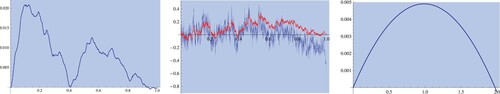We can easily adapt this expression to include the case of a general non-zero $\overline{\xi }\left(t\right)$ but the expression will be a lot messier due to the squared terms. We have found Monte Carlo to be the most efficient way to compute this triple integral in practice, which is what was used to compute the right plot in figure 1.

Figure 1. On the left we have plotted the optimal inventory $X_t^{\ast }$ in Theorem 2.2 when $P_t=\sigma {\int }_0^t(t-s{)}^{H-\frac{1}{2}}\mathrm{d}{W}_s$ is a Riemann-Liouville process using (26(26) $\begin{array}{rl}k(u,t)& =-\left(2c{\pi }^{\frac{3}{2}}{\tau }^{\frac{3}{2}}{\overline{u}}^{\frac{1}{4}}\mathrm{\Gamma }\right(H){)}^{-1}\cdot \left[\frac{{\tau }^{\frac{3}{2}+H}\sigma \mathrm{\Gamma }\left(\frac{1}{4}\right)\mathrm{\Gamma }\left(H_{\frac{1}{4}}\right)}{w^{\frac{1}{4}}(u-t)}\right.\\ & +H_{\frac{1}{4}}{\tau }^{\frac{1}{2}+H}{\overline{u}}^{-\frac{3}{4}+H}\sigma \mathrm{\Gamma }\left(\frac{1}{4}\right)\left(-B\left(\overline{u},-H_{\frac{1}{4}},\frac{3}{4}\right)\right.\\ & +\left.\frac{\mathrm{\Gamma }\left(\frac{3}{4}\right)\mathrm{\Gamma }\left(-H_{\frac{1}{4}}\right)}{\mathrm{\Gamma }(\frac{1}{2}-H)}\right)\mathrm{\Gamma }\left(H_{\frac{1}{4}}\right)\\ & \left.+\frac{\sqrt{2\pi }\mathrm{\Gamma }\left(H\right)({\tau }^{\frac{1}{2}+H}\sigma +\tau {\lambda }_1(u\left)\right)}{w^{\frac{1}{4}}}\right],\end{array}$(26) ) with $H=\frac{2}{3}$, $\sigma =1$, c = 1 and $\gamma =.5$ and $X_0=0$, and in the middle we have plotted $u_t^{\ast }$ (blue) and ${\xi }_t$ (in red). On the right, as a sanity check, we have plotted the expected profit/loss for α times the optimal trading speed, as a function of α (which we see is correctly maximized close to $\alpha =1$, the small numerical error is there because we have to estimate the triple integral in (24) with Monte Carlo).

2.5. Re-expressing the trading speed in terms of the price history

At the moment our optimal selling speed is expressed as $u_t={\int }_0^{t}k(u,t)\mathrm{d}{W}_u$, but it is more natural and useful to re-express $u_t$ in terms of P itself. To this end, let $Z_t={\int }_0^{t}g(s,t)\mathrm{d}{W}_s$, and we seek a function $h(\cdot ,\cdot )$ such that $h(t,t)Z_t-{\int }_0^t{h}_s(s,t)Z_s\mathrm{d}s=W_t$. Then we see that $\begin{array}{rl}& h(t,t)Z_t-{\int }_0^t{h}_s(s,t)Z_s\mathrm{d}s\\ & =h(t,t){\int }_0^{t}g(u,t)\mathrm{d}{W}_u-{\int }_0^t{h}_s(s,t){\int }_0^{s}g(u,s)\mathrm{d}{W}_u\mathrm{d}s\\ & =h(t,t){\int }_0^{t}g(u,t)-{\int }_0^t{\int }_u^t{h}_s(s,t)g(u,s)\mathrm{d}s\mathrm{d}{W}_u,\end{array}$ where $h_s(\cdot ,\cdot )$ denotes the partial derivative of h with respect to the first argument. Hence to find an inversion formula, we need to solve the integral equation $h(t,t)g(u,t)-{\int }_u^t{h}_s(s,t)g(u,s)\mathrm{d}s=1.$ If $g(s,t)=g(t-s)$ with $g\in L^2$ and we guess that $h(s,t)=h(t-s)$, then the equation takes the special form $h\left(0\right)g(t-u)+{\int }_u^t{h}^{\prime }(t-s)g(s-u)\mathrm{d}s=1.$ Setting $\tilde{s}=s-u$, we can re-write this as $h\left(0\right)g(t-u)+{\int }_0^{t-u}{h}^{\prime }(t-(u+\tilde{s}\left)\right)g\left(\tilde{s}\right)\mathrm{d}\tilde{s}=1,$ and replacing t−u with t we can further re-write as $h\left(0\right)g\left(t\right)+{\int }_0^t{h}^{\prime }(t-\tilde{s})g\left(\tilde{s}\right)\mathrm{d}\tilde{s}=h\left(0\right)g\left(t\right)+h^{\prime }\ast g=1.$ Then taking the Laplace transform, we have $h\left(0\right)\hat{g}+\widehat{\left(h^{\prime }\right)}\hat{g}=h\left(0\right)\hat{g}+(\lambda \hat{h}-h(0\left)\right)\hat{g}=\frac{1}{\lambda },$ so we see that (24) $\hat{h}=\frac{1}{{\lambda }^2\hat{g}}.$(24) Hence if $P_t={\int }_0^{t}g(t-u)\mathrm{d}{W}_u$ for some $g\in L^2$ then ${\xi }_t={\int }_0^t{K}_{\xi }(u,t)\mathrm{d}{W}_u$ with $K_{\xi }(u,t)=g(T-u)-g(t-u)$, and from the preceding computations we have the inversion formula $W_t=h(t,t)P_t-{\int }_0^t{h}_s(s,t)P_s\mathrm{d}s$ and recall that ${\hat{u}}_t={\int }_0^{t}k(u,t)\mathrm{d}{W}_u$ (where $k(\cdot ,\cdot )$ depends on $K_{\xi }$ via the Fredholm eq (12(12) $\begin{array}{rl}-K_{\xi }(u,t)& ={\int }_u^{T}G(|t-v|)k(u,v)\mathrm{d}v+\lambda \left(u\right)\end{array}$(12) ), and hence on g itself) so we now see how $\hat{u}$ depends solely on the (unaffected) stock price history $(P_u{)}_{0\le u\le t}$, which gives us our signal-adaptive optimal selling speed.

We can compute h explicitly for the case when $g\left(t\right)=t^{H-\frac{1}{2}}{\mathrm{e}}^{-\theta t}$ for $H\in (0,1)$, $\theta >0$ for which we find that (25) $\begin{array}{r}h\left(t\right)=\frac{\begin{array}{c}{\mathrm{e}}^{-\theta t}{t}^{-\frac{1}{2}-H}\left[\phantom{{\frac{1}{2}}^2}2-{\mathrm{e}}^{t\theta }(1+2H+2t\theta )\right.\\ \left.\left(E_{\frac{3}{2}+H}\left(t\theta \right)-\left(t\theta {)}^{\frac{1}{2}+H}\mathrm{\Gamma }\right(-\frac{1}{2}-H)\right)\right]\end{array}}{2\theta \mathrm{\Gamma }(-\frac{1}{2}-H)\mathrm{\Gamma }(\frac{1}{2}+H)}.\end{array}$(25) where $E_n\left(z\right)={\int }_1^{\mathrm{\infty }}\frac{{\mathrm{e}}^{-zt}}{t^n}\mathrm{d}t$. $H=\frac{1}{2}$ corresponds to the OU process for which $h\left(t\right)=1+\theta t$, and $\theta =0$ corresponds to the Riemann-Liouville process for which $h\left(t\right)=\frac{t^{\frac{1}{2}-H}}{\mathrm{\Gamma }(\frac{3}{2}-H)\mathrm{\Gamma }(\frac{1}{2}+H)}$ (see next section).

3. Examples and extensions of the main model

3.1. Rough signals

If $P_t=\sigma {\int }_0^t(t-s{)}^{H-\frac{1}{2}}\mathrm{d}{W}_s$ (i.e. a Riemann-Liouville process) for $H\in (0,1)$ and $\gamma =\frac{1}{2}$ and $\overline{\xi }\left(t\right)\equiv 0$ for simplicity, then clearly ${\xi }_t={\mathbb{E}}_t(P_T-P_t)={\int }_0^t\left(\right(T-s{)}^{H-\frac{1}{2}}-(t-s{)}^{H-\frac{1}{2}})\mathrm{d}{W}_s$ and (after some lengthy Mathematica computations) we find that (26) $\begin{array}{rl}k(u,t)& =-\left(2c{\pi }^{\frac{3}{2}}{\tau }^{\frac{3}{2}}{\overline{u}}^{\frac{1}{4}}\mathrm{\Gamma }\right(H){)}^{-1}\cdot \left[\frac{{\tau }^{\frac{3}{2}+H}\sigma \mathrm{\Gamma }\left(\frac{1}{4}\right)\mathrm{\Gamma }\left(H_{\frac{1}{4}}\right)}{w^{\frac{1}{4}}(u-t)}\right.\\ & +H_{\frac{1}{4}}{\tau }^{\frac{1}{2}+H}{\overline{u}}^{-\frac{3}{4}+H}\sigma \mathrm{\Gamma }\left(\frac{1}{4}\right)\left(-B\left(\overline{u},-H_{\frac{1}{4}},\frac{3}{4}\right)\right.\\ & +\left.\frac{\mathrm{\Gamma }\left(\frac{3}{4}\right)\mathrm{\Gamma }\left(-H_{\frac{1}{4}}\right)}{\mathrm{\Gamma }(\frac{1}{2}-H)}\right)\mathrm{\Gamma }\left(H_{\frac{1}{4}}\right)\\ & \left.+\frac{\sqrt{2\pi }\mathrm{\Gamma }\left(H\right)({\tau }^{\frac{1}{2}+H}\sigma +\tau {\lambda }_1(u\left)\right)}{w^{\frac{1}{4}}}\right],\end{array}$(26) where $H_{\frac{1}{4}}=H+\frac{1}{4}$, $\tau =T-u$, $w=\frac{T-t}{T-u}$, $\overline{u}=\frac{t-u}{T-u}$ and $B(z,a,b)={\int }_0^z{t}^{a-1}(1-t{)}^{b-1}\mathrm{d}t$ denotes the incomplete Beta function, and enforcing the liquidation condition ${\int }_u^{T}k(u,t)\mathrm{d}t=0$ we find that $\lambda \left(u\right)=-\mathrm{{\rm Y}}{\tau }^{H-\frac{1}{2}}$ where Υ is given by $\sigma \frac{\begin{array}{c}{\pi }^2\mathrm{c}\mathrm{s}\mathrm{c}\left(\theta \pi \right)+\mathrm{\Gamma }\left({\omega }_{-}\right)\left[2H\mathrm{\Gamma }{\left(\frac{3}{4}\right)}^2\mathrm{\Gamma }\left(H\right)-H\sqrt{\pi }\mathrm{\Gamma }\left(-\frac{1}{4}\right)\mathrm{\Gamma }\left(\theta \right)\right.\\ -\left.\pi \cos \left(H\pi \right)\mathrm{c}\mathrm{s}\mathrm{c}\left(\theta \pi \right)\mathrm{\Gamma }\left({\omega }_{+}\right)+\sqrt{\pi }\mathrm{\Gamma }\left(-\frac{1}{4}\right)\mathrm{\Gamma }\left(\frac{5}{4}+H\right)\right]\end{array}}{2H\mathrm{\Gamma }{\left(\frac{3}{4}\right)}^2\mathrm{\Gamma }\left({\omega }_{-}\right)\mathrm{\Gamma }\left(H\right)}$ with $\theta =\frac{1}{4}+H$ and ${\omega }_{\pm }=\frac{1}{2}\pm H$ (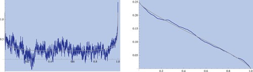see numerical simulations above and overleaf). Note that we have not rigourously verified that this strategy is admissible which would be extremely difficult to check (figures 2 and 3).

Figure 2. Non-Round trip case: from left to right (with $X_0=.25$ and the same parameters as above) we see (i) the optimal buying speed with no-signal (ii) $X_t^{\ast }$ with no signal.

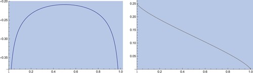
Figure 3. On the left we see the optimal selling speed with non-zero signal (blue) and the no-signal optimal speed (grey) and on the right we see $X_t^{\ast }$ with non-zero signal (blue) and zero signal (grey), for the same parameters and simulated Brownian motion as figure 2.

Remark 3.1

H can be efficiently estimated from a time series using maximum likelihood methods (see Chang 2014 for explicit formulae) or using convolutional neural networks (see Stone 2020).

3.2. Temporary price impact

If we add a temporary price impact term $\eta \dot{\phantom{a}}{X}_t=-\eta u_t$ on the right hand side of (1(1) $S_t=P_t+{\int }_0^{t}G(t-s)\mathrm{d}{X}_s,$(1) ), then we incur an additional $\eta u_t^2$ term in (3(3) $\tilde{V}\left(u\right)=-\mathbb{E}\left({\int }_0^T\left({\xi }_t+{\int }_0^{t}G(t-s)u_s\mathrm{d}s\right)u_t\mathrm{d}t\right).$(3) ), and a standard first order variational analysis of this expression leads to the following modified (4(4) ${\xi }_t+{\mathbb{E}}_t\left({\int }_0^{T}G(|t-v|)u_v\mathrm{d}v\right)=M_t\mathrm{a}.\mathrm{s}.$(4) ): ${\xi }_t+2\eta u_t^{\ast }+{\mathbb{E}}_t\left({\int }_0^{T}G(|t-v|)u_v^{\ast }\mathrm{d}v\right)=M_t$ for some martingale M to be determined such that $X_T=0$ as before. Then using the same ansatz $u_t={\int }_0^{t}k(u,t)\mathrm{d}{W}_u$, we can readily verify that (12(12) $\begin{array}{rl}-K_{\xi }(u,t)& ={\int }_u^{T}G(|t-v|)k(u,v)\mathrm{d}v+\lambda \left(u\right)\end{array}$(12) ) changes to $\begin{array}{rl}-K_{\xi }(u,t)& =2\eta k(u,t)+{\int }_u^{T}G(|t-v|)k(u,v)\mathrm{d}v+\lambda \left(u\right)-\overline{\xi }\left(t\right)\\ & =2\eta \overline{u}\left(t\right)+{\int }_0^{T}G(|t-v|)\overline{u}\left(v\right)\mathrm{d}v+{\lambda }_2\end{array}$ where $\lambda \left(u\right)$ and ${\lambda }_2$ are again chosen to ensure that $X_T=0$, and this is now a Fredholm equation of the second kind, for $u\in [0,T]$ fixed.

4. Calibrating the model to real limit order book data

To calibrate the price impact model in equation (1(1) $S_t=P_t+{\int }_0^{t}G(t-s)\mathrm{d}{X}_s,$(1) ) we employ the order flow of all market participants, the transaction prices weighted by volume, and the unaffected price process. We then look for parameters that best fit the data. In (1(1) $S_t=P_t+{\int }_0^{t}G(t-s)\mathrm{d}{X}_s,$(1) ) we refer to $P_t$ as the unaffected price process, and $\mathrm{d}{X}_t=-u_t\mathrm{d}t$ is the instantaneous trading of the agent. Let ${\tilde{P}}_t=P_t-{\int }_0^{t}G(t-s)\mathrm{d}{Y}_s$ be the “observable unaffected price”, where $\mathrm{d}{Y}_t=v_t\mathrm{d}t$ and Y is the cumulative instantaneous trading of all other market participants excluding the agent. Then (1(1) $S_t=P_t+{\int }_0^{t}G(t-s)\mathrm{d}{X}_s,$(1) ) changes to (27) $S_t={\tilde{P}}_t+{\int }_0^{t}G(t-s)\mathrm{d}{Z}_s$(27) where $\mathrm{d}{Z}_s=\mathrm{d}{X}_s+\mathrm{d}{Y}_s=(u_s+v_s)\mathrm{d}s$ captures the order flow of the entire market (see Cartea and Jaimungal 2016).

Given the previous decomposition, we show how to estimate the parameters that appear in the decay kernel G. Let Θ be the parameter space associated with G. For example, in the power-law impact case, in which $\theta =(c,\gamma )$, the parameter space is $\mathrm{\Theta }={\mathbb{R}}^{+}\times (0,1)$. Take $\theta \in \mathrm{\Theta }$ and consider a discretized version of (27(27) $S_t={\tilde{P}}_t+{\int }_0^{t}G(t-s)\mathrm{d}{Z}_s$(27) ) given by $S_{t_n}\approx {\tilde{P}}_{t_{n-1}}+\sum _{i=1}^n{G}^{\theta }(t_n-t_{i-1})(u_{t_i}+v_{t_i})\mathrm{\Delta }$ where $0=t_0<t_1<\cdots <t_n$, and $\mathrm{\Delta }=t_i-t_{i-1}$ for $i\in \{1,2,\dots ,n\}$. The quantity $(u_{t_i}+v_{t_i})\mathrm{\Delta }$ represents the volume traded in $[t_{i-1},t_i)$ by all market participants. The observable unaffected price ${\tilde{P}}_{t_{n-1}}$ can be taken to be the mid-price of the asset at time $t_{n-1}$, and $S_{t_n}$ is the volume-weighted average price of all transactions in $[t_{i-1},t_i)$.

Fix a given calibration horizon T (for example, one day of trading), let $t_0<t_1<\cdots <t_N$ be a fixed time grid, where $t_0=0$ and $t_N=T$ (for example, one minute intervals throughout the day), let $(S_{t_i}{)}_{1\le i\le N}$ be the observed volume-weighted transaction prices,¹ and let $(V_{t_i}{)}_{0\le i\le N}$ be the volume traded by all market participants. For instance, for $i\in \{1,2,\dots ,N\}$, $V_{t_i}=(u_{t_i}+v_{t_i})\mathrm{\Delta }$. Finally, let $({\tilde{P}}_{t_i}{)}_{0\le i\le N-1}$ be the mid-price sampled at times $t_0<t_1<\cdots <t_{N-1}$. We assume our observations have noise, that is to say $S_{t_n}={\tilde{P}}_{t_{n-1}}+\sum _{i=1}^n{G}^{\theta }(t_n-t_{i-1})V_{t_i}+{ϵ}_n,$ where $({ϵ}_n{)}_{n\in \mathbb{N}}$ is a collection of independent and identically distributed normal random variables. We take the estimator $\hat{\theta }$ of θ to be the parameters that minimize the residual sum of squares, in other words, (28) $\hat{\theta }={\mathrm{a}\mathrm{r}\mathrm{g}\mathrm{m}\mathrm{i}\mathrm{n}}_{\theta \in \mathrm{\Theta }}\sum _{n=1}^N{\left(S_{t_n}-{\tilde{P}}_{t_n}-\sum _{i=1}^n{G}^{\theta }(t_n-t_i)V_{t_i}\right)}^2.$(28) Next, we test the calibration method in (28(28) $\hat{\theta }={\mathrm{a}\mathrm{r}\mathrm{g}\mathrm{m}\mathrm{i}\mathrm{n}}_{\theta \in \mathrm{\Theta }}\sum _{n=1}^N{\left(S_{t_n}-{\tilde{P}}_{t_n}-\sum _{i=1}^n{G}^{\theta }(t_n-t_i)V_{t_i}\right)}^2.$(28) ). We employ limit order book (LOB) data from VOD, AAPL, and CSCO trading in NASDAQ from 2 December 2019 to 31 January 2020. The data comprise all of the updates in the best prices, quantities, and trades. We take the time intervals to be spaced by one minute, and we set $[0,T]$ to be from 10:00 am to 2:00 pm. We calibrate the parameters $(c,\gamma )$ in ${\mathbb{R}}^{+}\times (0,1)$ for the power-law impact case $G^{\theta }\left(t\right)=c{t}^{-\gamma }$, and we refer to the estimates as $\hat{c}$ and $\hat{\gamma }$. We observe that over the two months of data, the mean value (and standard deviation) of the estimate $\hat{\gamma }$ was 0.384 (0.104) for VOD, 0.440 (0.125) for AAPL, and 0.493 (0.104) for CSCO. Similarly, the mean value (and standard deviation) of the estimate $\hat{c}$ was 0.0015 (0.0004) for VOD, 0.0028 (0.0007) for AAPL, and 0.0009 (0.0004) for CSCO. For an alternate approach to the calibration of parameters under transient market impact, see Busseti and Lillo (2012).

Acknowledgments

We thank Alex Schied for helpful discussions.

Disclosure statement

No potential conflict of interest was reported by the author(s).

Notes

1 We define $S_0=P_0$. If there are no transactions in a given interval $[t_{i-1},t_i)$ for $i\in \{1,2,\dots ,N\}$, we define $S_{t_i}=S_{t_{i-1}}$. Otherwise, $S_{t_i}$ is the volume-weighted trade price over all trading carried in $[t_{i-1},t_i)$.

Appendix

Recall that $⟨u,v{⟩}_G=\mathbb{E}\left({\int }_0^T{\int }_0^T{u}_s{v}_{t}G\right(|t-s|\left)\mathrm{d}s\mathrm{d}t\right)$.

Lemma A.1

Let $u,v\in \mathcal{U}$ such that $\parallel u{\parallel }_G$ and $\parallel v{\parallel }_G$ are finite. Then $⟨u,v{⟩}_G<\mathrm{\infty }$.

Proof.

We first consider a deterministic function φ in the Schwarz space $\mathcal{S}$ with $\mathrm{s}\mathrm{u}\mathrm{p}\mathrm{p}\left(\phi \right)\subseteq [0,T]$ (φ will be replaced with a random $u\in {\mathcal{U}}_0^{X_0}$ below once we have the required machinery in place). Using Plancherel's theorem, we see that $\begin{array}{rl}⟨\phi ,\phi {⟩}_G& ={\int }_0^T\phi \left(t\right){\int }_0^T\phi \left(s\right)G(|t-s|)\mathrm{d}s\mathrm{d}t\\ & ={\int }_{-\mathrm{\infty }}^{\mathrm{\infty }}\phi \left(t\right){\int }_{-\mathrm{\infty }}^{\mathrm{\infty }}\phi \left(s\right)G(|t-s|)\mathrm{d}s\mathrm{d}t\\ & ={\int }_{-\mathrm{\infty }}^{\mathrm{\infty }}\hat{\phi }\left(k\right)\overline{\hat{\phi }\left(k\right)}\hat{G}\left(k\right)\mathrm{d}k\\ & ={\int }_{-\mathrm{\infty }}^{\mathrm{\infty }}|\hat{\phi }\left(k\right){|}^2\hat{G}\left(k\right)\mathrm{d}k\ge 0,\end{array}$ where $\hat{G}\left(k\right)=c_{\gamma }|k{|}^{\gamma -1}$ is the Fourier transform of G, for some constant $c_{\gamma }>0$. Thus $⟨\cdot ,\cdot {⟩}_G$ is a positive semi-definite bilinear form on $\mathcal{S}$. Using similar arguments to equation (8) in Forde and Smith (2020), we can also show $⟨\cdot ,\cdot {⟩}_G$ is continuous on the Schwarz space $\mathcal{S}\left(\mathbb{R}\right)$. Hence by Minlos's theorem, ${\mathrm{e}}^{-\frac{1}{2}⟨\phi ,\phi {⟩}_G}=\mathbb{E}\left({\mathrm{e}}^{i⟨\phi ,Z⟩}\right)$ is the characteristic functional of the Fractional Gaussian Field (FGF) Z with covariance function $G(|t-s|)=c|t-s{|}^{-\gamma }$ which lives in the space of tempered distributions ${\mathcal{S}}^{\prime }$ (see e.g. pg 8 of Janson 2009, and Duplantier et al. 2017 and Appendix A in Forde et al. 2020 for more details) which is the dual of the Schwartz space $\mathcal{S}$ (see e.g. Section 2.2 in Duplantier et al. 2014 and Theorem 2.1 in Bierme et al. 2017). Moreover, $\mathcal{S}$ is a Montel space and thus is reflexive, i.e. $({\mathcal{S}}^{\prime }{)}^{\prime }$ is isomorphic to $\mathcal{S}$ using the canonical embedding of S into its bi-dual $(S^{\prime }{)}^{\prime }$.

Proceeding as in Forde and Smith (2020), we now let $\overline{F}$ denote the Hilbert space equal to the $L^2(\mathcal{S},{\mathcal{F}}_T,\mathbb{P})$ closure of $F=\left\{Z\right(\phi ):\phi \in \mathcal{S},\mathrm{s}\mathrm{u}\mathrm{p}\mathrm{p}(\phi )\subseteq [0,T\left]\right\}$ where ${\mathcal{F}}_T=\sigma \left(\right(Z_u{)}_{0\le u\le T})$.

In order to characterize $\overline{F}$, we first note that $\mathbb{E}\left(\right(Z,\phi {)}^2)={\int }_0^T{\int }_0^{T}G(|t-s|\left)\phi \right(s\left)\phi \right(t)\mathrm{d}s\mathrm{d}t.$ We also know that $\begin{array}{rl}{\int }_0^T{\int }_0^{T}G(|t-s|)\phi \left(s\right)\psi \left(t\right)\mathrm{d}s\mathrm{d}t& =\mathbb{E}\left({\int }_{-\mathrm{\infty }}^{\mathrm{\infty }}\hat{\phi }\left(k\right)\overline{\hat{\psi }}\left(k\right)\hat{G}\left(k\right)\mathrm{d}k\right)\\ & =c_{\gamma }⟨\phi ,\psi {⟩}_{H^{-\frac{1}{2}(1-\gamma )}}\end{array}$ where $\hat{G}\left(k\right)=c_{\gamma }|k{|}^{\gamma -1}$ for some constant $c_{\gamma }$, and $H^s$ denotes the homogenous fractional Sobolev space of order s (see e.g. page 5 in Duchon et al. 2012 for definitions). Thus, setting $s=\frac{1}{2}(1-\gamma )$, the following two inner products on the linear space $\mathcal{S}$ of Schwarz functions are equivalent and hence generate the same topologies on $\mathcal{S}$:

1. $⟨\phi ,\psi {⟩}_{H^{-s}}:={\int }_{-\mathrm{\infty }}^{\mathrm{\infty }}|k{|}^{-2s}\hat{\phi }\left(k\right)\overline{\hat{\psi }}\left(k\right)\mathrm{d}k$ (i.e. the standard inner product on $H^{-s}$)

2. $⟨\phi ,\psi ⟩:=\mathbb{E}\left[Z\right(\phi \left)Z\right(\psi \left)\right]={\int }_0^T{\int }_0^T\phi \left(s\right)\psi \left(t\right)G(|t-s|)\mathrm{d}s\mathrm{d}t$.

We now make the following observations:

• Let $\phi \in H^{-s}$, with $\mathrm{s}\mathrm{u}\mathrm{p}\mathrm{p}\left(\phi \right)\subseteq [0,T]$. $\mathcal{S}$ is dense in $H^{-s}$, so there exists a sequence ${\phi }_n\in \mathcal{S}$ with $\mathrm{s}\mathrm{u}\mathrm{p}\mathrm{p}\left({\phi }_n\right)\subseteq [0,T]$ such that $\parallel {\phi }_n-\phi {\parallel }_{H^{-s}}\to 0$, and φ is a Cauchy sequence in $H^{-s}$ so (by the equivalence of norms) $Z\left({\phi }_n\right)$ is a Cauchy sequence in $\overline{F}$, and thus converges to some Y in $\overline{F}$. This defines $Z\left(\phi \right):=Y$ as a continuous linear extension of Z from $\mathcal{S}$ to the larger space $H^{-s}$, which we will also often write as $\int \phi \left(t\right)Z_t\mathrm{d}t$. To check that $Z\left(\phi \right)$ is uniquely specified, consider two such sequences ${\phi }_n$ and ${\phi }_n^{\prime }$. Then from the triangle inequality $\parallel {\phi }_n-{\phi }_n^{\prime }{\parallel }_{H^{-s}}\le \parallel {\phi }_n-\phi {\parallel }_{H^{-s}}+\parallel \phi -{\phi }_n^{\prime }{\parallel }_{H^{-s}}\to 0$ and thus (by the equivalence of norms) we have $\parallel Z\left({\phi }_n\right)-Z\left({\phi }_n^{\prime }\right){\parallel }_{L^2(\mathcal{S},{\mathcal{F}}_T,\mathbb{P})}=\parallel Z\left({\phi }_n\right)-Z\left({\phi }_n^{\prime }\right){\parallel }_{\overline{F}}\to 0.$

• Conversely, for any $Z\in \overline{F}$, there exists a sequence ${\phi }_n\in \mathcal{S}$ such that $Z\left({\phi }_n\right)$ converges to $Z\in L^2(\mathcal{S},{\mathcal{F}}_T,\mathbb{P})$, so ${\phi }_n$ is a Cauchy sequence with respect to the second norm defined above, and hence also a Cauchy sequence with respect to the $H^{-s}$ norm (by the equivalence of the two norms). $H^{-s}$ is a Hilbert space so Cauchy sequences in $H^{-s}$ converge i.e. there exists a φ in $H^{-s}$ such that ${\phi }_n\to \phi \in H^{-s}$.

Thus we have shown that $\overline{F}=\left\{Z\right(\phi ):\phi \in H^{-s},\mathrm{s}\mathrm{u}\mathrm{p}\mathrm{p}(\phi )\subseteq [0,T\left]\right\},$

where we are using the extension of Z to $H^{-s}$ on the right hand side here as defined in the first bullet point above. Moreover, we can now extend the inner product to $H^{-s}$ as $\begin{array}{rl}⟨\phi ,\psi ⟩& =\underset{n\to \mathrm{\infty }}{lim}\mathbb{E}\left[Z\right({\phi }_n\left)Z\right({\psi }_n\left)\right]\\ & =\underset{n\to \mathrm{\infty }}{lim}{\int }_0^T{\int }_0^T{\phi }_n\left(s\right){\psi }_n\left(t\right)G(|t-s|)\mathrm{d}s\mathrm{d}t\end{array}$ where ${\phi }_n,{\phi }_n\in \mathcal{S}$ and ${\phi }_n\to \phi$ in $H^{-s}$ and ${\psi }_n\to \psi$ in $H^{-s}$.

Finally, to prove the lemma, if $u\in {\mathcal{U}}_0^{X_0}$ and $\mathbb{E}\left({\int }_0^T{\int }_0^T{u}_s{u}_{t}G\right(|t-s|\left)\mathrm{d}s\mathrm{d}t\right)<\mathrm{\infty }$, then ${\int }_0^T{\int }_0^T{u}_s{u}_{t}G(|t-s|)\mathrm{d}s\mathrm{d}t<\mathrm{\infty }$ a.s., so $u\in H^{-s}$ a.s. Then if we assume the field Z is independent of u then $\begin{array}{rl}⟨u,v{⟩}_G& =\mathbb{E}\left(\right(Z,u\left)\right(Z,v\left)\right)\le \mathbb{E}\left(\right(Z,u{)}^2{)}^{\frac{1}{2}}\mathbb{E}\left(\right(Z,v{)}^2{)}^{\frac{1}{2}}\\ & =\mathbb{E}\left(\mathbb{E}\right((Z,u{)}^2|u){)}^{\frac{1}{2}}\mathbb{E}\left(\mathbb{E}\right((Z,v{)}^2{)}^{\frac{1}{2}})\\ & =\mathbb{E}{\left({\int }_0^T{\int }_0^T{u}_s{u}_{t}G(|t-s|)\mathrm{d}s\mathrm{d}t\right)}^{\frac{1}{2}}\\ & \times \mathbb{E}{\left({\int }_0^T{\int }_0^T{v}_s{v}_{t}G(|t-s|)\mathrm{d}s\mathrm{d}t\right)}^{\frac{1}{2}}\\ & <\mathrm{\infty }\end{array}$ as required.

References

- Almgren, R. and Chriss, N., Optimal execution of portfolio transactions. J. Risk, 2001, 3, 5–50. doi: https://doi.org/10.21314/JOR.2001.041
- Bank, P., Soner, H.M. and Voß, M., Hedging with temporary price impact. Math. Financ. Econ., 2017, 11(2), 215–239. doi: https://doi.org/10.1007/s11579-016-0178-4
- Belak, C., Muhle-Karbe, J. and Ou, K., Liquidation in target zone models. Market Micro. Liquid., 2020, 4(3 Article ID 1950010
- Bierme, H., Durieu, O. and Wang, Y., Generalized random fields and Lévy's continuity theorem on the space of tempered distributions. Preprint, 2017.
- Busseti, E. and Lillo, F., Calibration of optimal execution of financial transactions in the presence of transient market impact. J. Stat. Mech. Theory Exp., 2012, 2012, Article ID P09010. doi: https://doi.org/10.1088/1742-5468/2012/09/P09010
- Cartea, A. and Jaimungal, S., Incorporating order-flow into optimal execution. Math. Financ. Econ., 2016, 10(3), 339–364. doi: https://doi.org/10.1007/s11579-016-0162-z
- Cartea, A., Jaimungal, S. and Penalva, J., Algorithmic and High-Frequency Trading, 2015 (Cambridge University Press: Cambridge).
- Cartea, A., Donnelly, R. and Jaimungal, S., Enhancing trading strategies with order book signals. Appl. Math. Finance, 2018, 25(1), 1–35. doi: https://doi.org/10.1080/1350486X.2018.1434009
- Cartea, A., Perez Arribas, I. and Sánchez-Betancourt, L., Optimal execution of foreign securities: A double-execution problem with signatures and machine learning. Preprint, 2020.
- Chakrabarti, A. and George, A.J., A formula for the solution of general Abel integral equation. Appl. Math. Lett., 1994, 7(2), 87–90. doi: https://doi.org/10.1016/0893-9659(94)90037-X
- Chang, Y.C., Efficiently implementing the maximum likelihood estimator for hurst exponent. Math. Probl. Eng., 2014, 2014, Article ID 490568.
- Curato, G., Gatheral, J. and Lillo, F., Optimal execution with nonlinear transient market impact. Quant. Finance, 2017, 17(1), 41–54. doi: https://doi.org/10.1080/14697688.2016.1181274
- Dang, N.-M., Optimal execution with transient impact, 2014. Available at SSRN 2183685.
- Duchon, J., Robert, R. and Vargas, V., Forecasting volatility with the multifractal random walk model. Math. Finance, 2012, 22(1), 83–108. doi: https://doi.org/10.1111/j.1467-9965.2010.00458.x
- Duplantier, D., Rhodes, R., Sheffield, S. and Vargas, V., Renormalization of critical Gaussian multiplicative chaos and KPZ relation. Comm. Math. Phys., August, 2014, 330(1), 283–330. doi: https://doi.org/10.1007/s00220-014-2000-6
- Duplantier, D., Rhodes, R., Sheffield, S. and Vargas, V., Log-correlated Gaussian fields: An overview. In Geometry, Analysis and Probability, pp. 191–216, August, 2017.
- Forde, M. and Smith, B., The conditional law of the Bacry-Muzy and Riemann-Liouville log-correlated Gaussian fields and their GMC, via Gaussian Hilbert and fractional Sobolev spaces. Stat. Prob. Lett., June, 2020, 161, Article 108732. doi: https://doi.org/10.1016/j.spl.2020.108732
- Forde, M. and Zhang, H., Asymptotics for rough stochastic volatility models. SIAM J. Financ. Math., 2017, 8, 114–145. doi: https://doi.org/10.1137/15M1009330
- Forde, M., Fukasawa, M., Gerhold, S. and Smith, B., The Rough Bergomi model as H→0 – skew flattening/blow up and non-Gaussian rough volatility. Preprint, 2020.
- Gatheral, J., Schied, A. and Slynko, A., Transient linear price impact and Fredholm integral equations. Math. Finance, 2012, 22, 445–474. doi: https://doi.org/10.1111/j.1467-9965.2011.00478.x
- Janson, S., Gaussian Hilbert Spaces, 2009 (Cambridge University Press: Cambridge).
- Kalsi, J., Lyons, T. and Arribas, I.P., Optimal execution with rough path signatures. SIAM J. Financ. Math., 2020, 11(2), 470–493. doi: https://doi.org/10.1137/19M1259778
- Lorenz, C. and Schied, A., Drift dependence of optimal trade execution strategies under transient price impact. Finance Stoch., 2013, 17, 743–770. doi: https://doi.org/10.1007/s00780-013-0211-x
- Neuman, E. and Voß, M., Optimal signal-adaptive trading with temporary and transient price impact. Preprint, 2020.
- Obizhaeva, A. and Wang, J., Optimal trading strategy and supply/demand dynamics. J. Finance Markets, 2013, 16(1), 1–32. doi: https://doi.org/10.1016/j.finmar.2012.09.001
- Porter, D. and Stirling, D.S.G., Integral Equations: A Practical Treatment from Spectral Theory to Applications, 1990 (Cambridge University Press: Cambridge).
- Stone, H.M.C, Calibrating rough volatility models: A convolutional neural network approach. Quant. Finance, 2020, 20(3), 379–392. doi: https://doi.org/10.1080/14697688.2019.1654126
Appendix
Recall that .
Lemma A.1
Let such that
and
are finite. Then