Lifetime consumption and investment with housing, deferred annuities and home equity release

Abstract

We develop a life-cycle optimal investment and consumption model with deferred annuities, housing, mortgages and home equity release. The investor can hold cash, bonds, stocks, annuities and can invest in housing, through renting, purchasing, or a mix of both, with access to variable-rate mortgages. In retirement, the investor can access his housing equity through a form of home equity release called a home reversion contract. Transaction costs, taxes and management fees are explicitly included. The investor's risk preferences are represented by standard power utility derived from housing and non-housing consumption, both before and after retirement, and from bequest. We use multi-stage stochastic programming to solve the optimization problem numerically. Our results show that both non-housing and housing consumption may be higher in retirement when deferred annuities and home reversion are available than when they are absent. The bequest motive has little effect on home reversion and results in a small reduction in overall annuitization.

Keywords:

• Stochastic programming
• Retirement planning
• Home equity reversion
• Deferred annuities

JEL Classification:

• C61
• E21
• G11

1. Introduction

During an individual's financial life-cycle, consumption and investment decisions have to be made regarding housing and retirement planning. Housing is a consumption good since utility is derived from owning or renting residential property. If owned, housing is also a part of the individual's investment portfolio, as a marketable risky asset, when a residential property is bought either with or without a mortgage. The 2016 Survey of Consumer Finances reports that U.S. households' primary residence was worth US$24.2 trillion, amounting to 24% of total assets held by households (Federal Reserve Board 2016). Because of its sheer monetary value, and the leverage with which it is bought, housing often dominates both consumption and investment, but is a significant missing component in standard life-cycle models (Cocco 2005, Campbell 2006, Kraft et al. 2018).

By the time a home-owner retires, he will typically have paid off any home loan and may wish to access the large amount of equity that he has in his residence in order to smooth consumption over time. It turns out that home-owning retirees can release the equity in their homes, without selling or down-sizing their homes, by purchasing products such as reverse mortgages and home reversions. These home equity release products can be an important source of income for retirees (Hanewald et al. 2016). As of October 2019, a total of 1,137,055 reverse mortgages have been sold under the U.S. federal Home Equity Conversion Program since the program's inception with the National Housing Act of 1987 (NRMLA 2019).

Income in retirement is principally secured through retirement plans (as well as social security). Retirement plans involve long-term saving and investment with assets accumulating over decades. According to the 2016 Survey of Consumer Finances, retirement accounts in the U.S. were worth US$15 trillion, which represents 15% of households' total assets (Federal Reserve Board 2016). Retirement planning includes investment in life-contingent income products, such as annuities of various kinds, which provide stable lifetime income beginning at a pre-specified date, in most cases at retirement or at an advanced age (Horneff et al. 2010, Maurer et al. 2013). Sales of annuities totaled $203.5 billion in 2017 in the U.S. (Chen et al. 2019).

The bulk of life-cycle research tends to involve highly stylized models with restricted investment choices, and limited consideration of transaction costs and other frictions. These models typically exclude the combination of housing and annuities, although these are important to investors in the real world. Our main contribution is to address this gap in the literature and determine the optimal life-cycle decisions for individuals in a realistic setting, where housing, mortgages, home equity release and annuities (immediate and deferred) are available, in addition to the usual financial assets (cash, bonds, equities). We replicate empirical findings in terms of equity allocation over the life-cycle and find that home equity release and deferred annuities can boost housing and non-housing consumption in retirement, even with a bequest motive present.

In this paper, we use multi-stage stochastic programming (MSP), a method very commonly used in operations research. MSP enables us to integrate a financial market, an annuity market, a housing market and a home equity release product, as well as realistic constraints such as no short sales, maximum loan-to-value ratios on mortgages, income taxes, transaction costs and management fees. Our optimization problem has a non-linear objective function with linear constraints. For an individual retirement planning problem with the application of MSP, refer to Dempster (2011), Consigli et al. (2012), and Konicz et al. (2016). In particular, we extend the approach of Konicz et al. (2016) by including deferred annuities, housing services and home reversion products in the individual retirement planning problem.

The rest of this paper is organized as follows. In Section 2, we present an overview of housing, home equity release and annuity products. In Section 3, the financial market model consisting of equity returns and yield curves based on the Vasicek model is defined. This underlies our multi-stage portfolio optimization problem. We also present the annuity and house price models. A description of the individual's lifetime investment optimization problem is given in Section 4. Further, in Section 5, we formulate the multi-stage stochastic programming problem and in Section 6, we investigate the numerical solutions to the portfolio optimization problem using five different product mixes of immediate and deferred annuities, and home reversion contracts. We also provide an economic interpretation for our numerical analysis.

2. Background and literature review

In this section, we discuss housing in an individual's life-cycle investment. We also introduce home equity release products, in particular home reversion contracts. Annuities, immediate and deferred, are important products that generate income for retirees and are also discussed.

2.1. Housing

The life-cycle literature shows that housing, with risky price dynamics, has a large effect on the consumption and investment decisions made by a rational individual over his lifetime. Standard life-cycle models without housing, for example by Viceira (2001) and Cocco et al. (2005), predict that equity holdings decline as individuals age, particularly if labour income is risk-free and bond-like, as human capital falls with age. The empirical data show the opposite, with stock holding increasing with age before retirement (Cocco 2005). Flavin and Yamashita (2002) and Cocco (2005) find that, when housing is an available asset, relatively young individuals invest a low proportion of their wealth in stocks because they have to pay off their mortgage and because their house can itself be regarded as a risky asset holding. Cocco (2005) also shows that housing market risk crowds out stock market investment, with this effect being more prominent for lower net-worth individuals (who will also typically be younger).

Yao and Zhang (2005) distinguish between owning and renting property. They also introduce a bequest motive when an individual dies and leaves wealth to his heirs, net of the costs of selling his house. Like Cocco (2005), they also find that home-owning investors hold less stocks as a proportion of their net worth, compared to renters, because stock market risk is replaced by housing risk. Kraft and Munk (2011) conclude that the young prefer to rent initially to moderate risk, since housing and labour income are positively correlated, but that home ownership increases with age. Kraft et al. (2018) add habit formation in housing consumption, and find that empirical life-cycle patterns are reproduced: initially, housing dominates and stock market investments are low, but stock holdings then increase with age and then decline in retirement; non-housing consumption is likewise hump-shaped. The housing habit requires the investor to hold a wealth buffer, in effect, and younger investors can ill-afford stock market risk to this wealth buffer.

2.2. Home equity release products

These products can be broadly classified into two types, reverse mortgages and home reversion contracts, and we briefly review them here. For more detail, see Alai et al. (2014) and Hanewald et al. (2016).

Reverse mortgages involve debt. Using a reverse mortgage product, a home-owner can borrow a certain amount of money (usually as a lump sum but possibly also as an annuity) with his house as collateral. No interest is paid and the loan balance is rolled up at a fixed or adjustable interest rate. The owner retains the right to live in his home until he dies (or moves permanently out), at which point the reverse mortgage is repaid by selling the house. The reverse mortgage provider offers a no negative equity guarantee, also known as non-recourse provision, i.e. the loan balance cannot exceed the sale price of the house.

Home reversion contracts involve the transfer of equity; no new debt is incurred. The home-owner sells all or a portion of his home to the home reversion provider and receives a lump sum as well as a lifetime lease contract which enables him to stay in his property until death. Reverse mortgages are more popular than home reversion plans, but they are both available in the U.S., the U.K., Australia, Canada, as well as several European countries (Alai et al. 2014, Hanewald et al. 2016). In this paper, we will consider the home reversion contract.

The use of home equity release products is an important decision for an individual investor, but there are few studies on this topic. Most of these tend to be focused on the distributional advantages of retirees' income rather than the lifetime investment decisions. A reverse mortgage which pays an annuity, rather than a lump sum, does not increase most retirees' income by much, but it can be a significant component of income for an older retiree whose life expectancy is very short. On the other hand, a reverse lump-sum mortgage can help home-owners diversify wealth and reduce exposure to a single and illiquid house asset (Venti and Wise 1991, Mayer and Simons 1994). Alai et al. (2014) find that a home reversion contract is more profitable and less risky for the provider than a reverse mortgage if the loan-to-value (LTV) is greater than 50%, but that it is the other way round if the LTV is less than 50%. Hanewald et al. (2016) conclude that both types of home equity release products are welfare-enhancing for individuals, with the reverse mortgage being better because it supplies a higher lump sum and protects against house price declines. However, their model is highly stylized: it is a two-period model, with a single financial asset (cash) and with interest rate and house price growth being independent of each other and i.i.d.

2.3. Annuity products

An annuity makes a regular stream of payments to the annuity-holder while he is alive. It is sold by life insurers to individuals for retirement planning purposes since annuities provide an income for life and mitigate retirees' longevity risk, i.e. the risk that retirees will outlive their savings. Deferred annuities comprise a deferment period between the purchase date of the annuity and its first payment date. If the deferment period is zero, the deferred annuity is known as an immediate annuity. In this paper, the individual investor can purchase deferred annuities, and we use this term to encompass immediate annuities.

Most life-cycle research has been limited to immediate annuities: see for example Koijen et al. (2011). However, deferred annuities can be very useful to reduce longevity risk at very old ages (Scott 2008, Ezra 2016). Horneff et al. (2010) and Maurer et al. (2013) also show that they can help younger working individuals secure a retirement income well before retirement: the optimal strategy is to buy deferred annuities from the age of 40 and to continue buying them using up to 80% of wealth at retirement. Huang et al. (2016) assume a mean-reverting interest rate and show that the optimal strategy for a risk-averse agent is to start buying deferred annuities at a lower boundary of interest rates and invest all wealth in deferred annuities when the interest rate reaches an upper boundary.

3. Market structure

The assumptions that we make about financial assets are described in this section. We also describe annuities, housing, mortgages and home reversion contracts and we explain how these are modelled in relation to the financial market.

3.1. Financial markets

We consider an investor who is allowed to invest in cash, bond funds and equity funds, denoted by C, B and E, respectively. Let $S_{i,t}$, $i=\{C,B,E\}$ be the price at time t of a unit¹ in the cash, bond and equity funds, respectively. In order to incorporate interest rate uncertainty in our framework, a stochastic term structure model is required. We use the Vasicek mean-reverting process to model the short rate $r_t$, (1) $\text{d}{r}_t=\nu (\tilde{\theta }-r_t)\text{d}t+{\sigma }_0\text{d}{W}_{r,t},$(1) where $\nu >0$ is the speed of reversion to the mean level $\tilde{\theta }$, ${\sigma }_0$ is the volatility and $r_0>0$.

The stock price (the price of a unit in the equity fund) $S_{E,t}$ is given by (2) $\text{d}{S}_{E,t}=(r_t+{\mu }_E)S_{E,t}\text{d}t+{\sigma }_E{S}_{E,t}\text{d}{W}_{E,t},$(2) where ${\mu }_E$ is the risk premium, ${\sigma }_E>0$ is the volatility. $W_{E,t}$ and $W_{r,t}$ are correlated Wiener processes, with correlation coefficient ${\rho }_{EB}$: (3) $\text{d}{W}_{r,t}=\text{d}{\tilde{W}}_{1,t},\text{d}{W}_{E,t}={\rho }_{EB}\text{d}{\tilde{W}}_{1,t}+\sqrt{1-{\rho }_{EB}^2}\text{d}{\tilde{W}}_{2,t},$(3) where ${\tilde{W}}_{1,t}$ and ${\tilde{W}}_{2,t}$ are independent Wiener processes.

The individual can rebalance his portfolio, as well as buy deferred annuities, at regular intervals of length $\mathrm{\Delta }t$ years. There are $N\in \mathbb{N}$ such regular intervals in his lifetime $[0,\tau )$. Defining $R_{i,t}$ as the continuously compounded return of asset $i\in \{C,B,E\}$ from time $t-\mathrm{\Delta }t$ to t, the price $S_{i,t}$ of asset i evolves according to the following: (4) $S_{i,t}=S_{i,t-\mathrm{\Delta }t}\cdot \exp \left(R_{i,t}\right),$(4) where $S_{i,0}=1$ without loss of generality.

The return of the cash fund over the time period $(t-\mathrm{\Delta }t,t)$ is simply the accumulated spot rates defined by the Vasicek model, i.e. $R_{C,t}={\int }_{t-\mathrm{\Delta }t}^t{r}_s\text{d}s$. This can be substituted into (4(4) $S_{i,t}=S_{i,t-\mathrm{\Delta }t}\cdot \exp \left(R_{i,t}\right),$(4) ) to give $S_{C,t}$, the price of a unit of the cash fund.

Using the price of a zero-coupon bond in the Vasicek model, the gross return of the long-term bond fund with a maturity of M years over a holding period of length $\mathrm{\Delta }t$ from time $t-\mathrm{\Delta }t$ to t is approximated by (5) $R_{B,t}=a(M-\mathrm{\Delta }t)-a\left(M\right)-b(M-\mathrm{\Delta }t)r_t+b\left(M\right)r_{t-\mathrm{\Delta }t},$(5) where $b\left(M\right)=(1-e^{-\nu M})/\nu$ and $a\left(M\right)=(\tilde{\theta }+{\mu }_0-{\sigma }_0^2/2{\nu }^2)\left(b\right(M)-M)-{\sigma }_0^{2}b(M{)}^2/4\nu$, and ${\mu }_0$ relates to the market price of interest rate risk. Accordingly, the price dynamics of the bond fund is obtained by substituting $R_{B,t}$ from (5(5) $R_{B,t}=a(M-\mathrm{\Delta }t)-a\left(M\right)-b(M-\mathrm{\Delta }t)r_t+b\left(M\right)r_{t-\mathrm{\Delta }t},$(5) ) into (4(4) $S_{i,t}=S_{i,t-\mathrm{\Delta }t}\cdot \exp \left(R_{i,t}\right),$(4) ).

3.2. Annuity market

In our model, the individual investor can also buy deferred annuities while in retirement. The deferred annuities are priced in terms of the term structure model introduced in section 3.1. Suppose that the investor is aged δ at time 0. For practical purposes, we also assume that a person cannot live beyond age ω, which is the maximum age in an actuarial life table, so the individual investor dies before or at time $\tau =\omega -\delta$.

We use the standard actuarial notation for survival and death probabilities. The probability that a person aged $\delta +t$ years survives for m years until age $\delta +t+m$ is denoted by ${}_m{p}_{\delta +t}$. The probability that a $\delta +t$-year old person dies over the following $\mathrm{\Delta }t$ years is denoted by ${}_{\mathrm{\Delta }t}{q}_{\delta +t}$, abbreviated to $q_{\delta +t}$ when $\mathrm{\Delta }t=1$. The probability that a $\delta +t$-year old person survives for m years and then dies within the next $\mathrm{\Delta }t$ years is $\left[m\right]\delta +t\cdot \left[\mathrm{\Delta }t\right]\delta +t+m$, denoted by $\left[m|\mathrm{\Delta }t\right]\delta +t$.

We use $A\left(\psi \right)$ to denote a deferred annuity which starts to pay an annual income of $1 at age ψ until death. Let the price at time t of such an annuity be $S_{A\left(\psi \right),t}$. For a policyholder aged $\delta +t$ at time t, the fair actuarial price of a deferred annuity contract paying $1 of annual income for lifetime from age ψ is (6) $S_{A\left(\psi \right),t}=\sum _{m=\psi -\delta -t}^{\tau -t-1}{}_m{p}_{\delta +t}\exp \left(a\left(m\right)-b\left(m\right)r_t\right).$(6) It is also convenient to state the price of a whole-life immediate insurance contract which pays $1 to a beneficiary upon the policyholder's death: (7) $S_{W,t}=\sum _{m=0}^{\tau -t-1}\left[m|\right]\delta +t\exp \left(a\left(m\right)-b\left(m\right)r_t\right).$(7) We assume static pricing mortality rates here and ignore any loading factor that an insurer might include to cover expenses.

3.3. Housing market and mortgage

We follow the approach of Kraft and Munk (2011) and Kraft et al. (2018) and assume that the housing market is divisible in a number of ‘units’. A housing unit represents a quantum of housing in terms of size, quality and location, so that a house can consist of, say, 50 units. Individuals can buy or rent a combination of these units. We use H to denote the housing market, D to denote the mortgage debt, and we introduce the following notation and definitions:

1. Let $S_{H,t}$ be the price of a housing unit at time t, and $H_t$ be the number of such units consumed at time t. Then, the amount of housing consumed at time t is $H_t{S}_{H,t}$.

2. Of the $H_t$ housing units that are consumed, the individual can directly own $X_{HA,t}$ units as an asset and can also rent $X_{HR,t}$ units from a landlord. If this represents a single house, then this is equivalent to mixed, or shared, ownership. Thus, $H_t=X_{HA,t}+X_{HR,t}$.

3. The rent that is paid on rented housing is directly proportional to the housing price unit at a constant rate ${\phi }_{HR}^u$ paid upfront (in advance) (Yao and Zhang 2005, Kraft and Munk 2011).

4. The monetary value $X_{HA,t}{S}_{H,t}$ of housing units directly owned by the individual may be financed by mortgage debt with outstanding balance $D_{H,t}$. The difference $X_{HA,t}{S}_{H,t}-D_{H,t}$ is the individual's own equity in housing. The mortgage provider imposes a loan-to-value ratio of ${\mathrm{\Lambda }}_{LTV}$, so $D_{H,t}\le X_{HA,t}{S}_{H,t}{\mathrm{\Lambda }}_{LTV}$, in the absence of home equity release.

5. The number of housing units purchased at time t with a newly issued mortgage is $X_{HD,t}$.

6. The mortgage is an interest-only mortgage with flexible repayment of principal. At time t, mortgage interest $D_{I,t}$ must be paid at a variable rate $r_t+\alpha$, where α is a mortgage rate premium. The individual is free to choose the principal repayment $D_{P,t}$ at time t, except at the maturity of the mortgage when all principal must be repaid in full.

Prior to retirement, the housing situation of an individual can be summarized as in Table 1, where $S_{H,t}$ represents the value of one unit of housing at time t:

Table 1. Description of housing variables for an individual prior to retirement.

Housing	Rented	Total owned	Owned (mortgage)	Owned (outright)
No. of units	$X_{HR,t}$	$X_{HA,t}$	$D_{H,t}/S_{H,t}$	$X_{HA,t}-D_{H,t}/S_{H,t}$
Value	$X_{HR,t}{S}_{H,t}$	$X_{HA,t}{S}_{H,t}$	$D_{H,t}$	$X_{HA,t}{S}_{H,t}-D_{H,t}$

In the lifetime finance literature, the geometric Brownian motion (GBM) is commonly used to model house prices (Kraft and Munk 2011, Kraft et al. 2018). We ignore the short-run autocorrelation that is observed in the real estate markets (Gau 1987, Case and Shiller 1988). We assume that the market is efficient in the long run so that the GBM can be used for pricing home equity release (Weinrobe 1988, Szymanoski 1994, Wang et al. 2008). The price $S_{H,t}$ of one unit of housing is given by (8) $\text{d}{S}_{H,t}=(r_t+{\mu }_H)S_{H,t}\text{d}t+{\sigma }_H{S}_{H,t}\text{d}{W}_{H,t},$(8) where ${\mu }_H$ is the risk premium on the house price, $r_t$ is the short interest rate in (1(1) $\text{d}{r}_t=\nu (\tilde{\theta }-r_t)\text{d}t+{\sigma }_0\text{d}{W}_{r,t},$(1) ), and ${\sigma }_H>0$ is the constant price volatility. The Wiener processes $W_{r,t}$, $W_{E,t}$ and $W_{H,t}$ in (1(1) $\text{d}{r}_t=\nu (\tilde{\theta }-r_t)\text{d}t+{\sigma }_0\text{d}{W}_{r,t},$(1) ), (2(2) $\text{d}{S}_{E,t}=(r_t+{\mu }_E)S_{E,t}\text{d}t+{\sigma }_E{S}_{E,t}\text{d}{W}_{E,t},$(2) ) and (8(8) $\text{d}{S}_{H,t}=(r_t+{\mu }_H)S_{H,t}\text{d}t+{\sigma }_H{S}_{H,t}\text{d}{W}_{H,t},$(8) ) are correlated. The correlation coefficient of housing returns with bond returns and equity returns are ${\rho }_{HB}$ and ${\rho }_{HE}$, respectively: (9) $\text{d}{W}_{H,t}={\rho }_{HB}\text{d}{\tilde{W}}_{1,t}+{\hat{\rho }}_{HE}\text{d}{\tilde{W}}_{2,t}+\sqrt{1-{\rho }_{HB}^2-{\hat{\rho }}_{HE}^2}\text{d}{\tilde{W}}_{3,t},$(9) where ${\hat{\rho }}_{HE}=({\rho }_{HE}-{\rho }_{EB}{\rho }_{HB})/\surd (1-{\rho }_{EB}^2)$, and ${\tilde{W}}_{1,t}$, ${\tilde{W}}_{2,t}$ and ${\tilde{W}}_{3,t}$ are independent Wiener processes.

This house price model is also used by Kraft and Munk (2011), except that they include correlation with stochastic labour income, whereas labour income is deterministic in our model. (However, they have neither annuities nor home equity release.) Other house price models are possible, such as the ARIMA-GARCH model of Chen et al. (2010), and regression and non-regression-based models described by Case and Quigley (1991) and Shao et al. (2015, 2018).

3.4. Home reversion contract

Once retired, the individual investor can enter into a home reversion contract, the broad features of which are described in section 2.2. The pricing of a home reversion contract depends on the appraised value of the house, and the individual's age and gender (single- or joint-life). Age and gender determine mortality rates, which may be obtained from a static discrete mortality table (Weinrobe 1988, Szymanoski 1994), a static continuous function like the Gompertz model (Alai et al. 2014, Cho et al. 2015), or a stochastic model like Lee-Carter (Wang et al. 2008, Chen et al. 2010). Static models neglect uncertain mortality improvements, of course.

Assume that the notional lease payments, under the lease associated with the home reversion plan, are paid in advance annually at the lease rate ${\phi }_R^l$. A fair actuarial value of the lump-sum payment of a home reversion contract per housing unit is: (10) $\begin{array}{rl}{S}_{R,t}& =\sum _{m=0}^{\tau -t}\left(\left[m|\right]\delta +t-\left[m\right]\delta +t{\phi }_R^l\right)\exp \left(a\right(m)-b(m\left)r_t\right)\\ & \times \mathbb{E}\left[S_{H,t+m}\right|S_{H,t}].\end{array}$(10) The lump sum paid to the home-owner equals the expected present value of a life insurance paying out the price of the house when the home-owner dies, reduced by the expected present value of a notional annuity made up of the annual lease payments while the home-owner is alive.

Before retirement, an individual can only own property (outright or through a mortgage) and rent property. After retirement, an individual can also choose to release some of their equity in a property to a home reversion provider. At time t, they can choose to release $X_{R,t}$ housing units, which they previously owned outright.

Post-retirement, the housing situation of an individual can therefore be summarized as in Table 2.

Table 2. Description of housing variables for an individual post-retirement.

Housing	Rented	Total owned	Owned (mortgage)	Equity released	Owned (outright)
No. of units	$X_{HR,t}$	$X_{HA,t}$	$D_{H,t}/S_{H,t}$	$X_{R,t}$	$X_{HA,t}-X_{R,t}-D_{H,t}/S_{H,t}$
Value	$X_{HR,t}{S}_{H,t}$	$X_{HA,t}{S}_{H,t}$	$D_{H,t}$	$X_{R,t}{S}_{H,t}$	$X_{HA,t}{S}_{H,t}-X_{R,t}{S}_{H,t}-D_{H,t}$

4. Lifetime investment

Consider an individual who has a lifetime investment plan with the timeline shown in Table 3. Let ${\tau }_M$ be the random age of death of the individual. We introduce some notation below and emphasize the key features of this investment plan:

1. The timeline ends at time τ, which is the final age in an actuarial lifetable, included for practical reasons: $0<{\tau }_M\le \tau$. Investment planning ends at a planning horizon $\mathcal{T}<\tau$, included here for modelling purposes.

2. During lifetime $[0,{\tau }_M)$, the individual earns utility $u\left(C_t^{1-\theta }{H}_t^{\theta }\right)$ from non-housing consumption $C_t$ as well as housing consumption $H_t$ where housing consumption can be through either ownership or rental. We assume a power utility function $u\left(x\right)=x^{1-\gamma }/(1-\gamma )$, with risk aversion coefficient γ.

3. During investment planning lifetime $[0,{\tau }_M\wedge \mathcal{T})$, the individual can

   1. trade housing units. He may acquire a mortgage to finance any housing unit purchase, and thereafter pay interest $D_{I,t}$ on the mortgage balance $D_{H,t}$, with flexible repayment $D_{P,t}$ of principal.

   2. trade units in cash, bond and equity funds, each unit being worth $S_{C,t}$, $S_{B,t}$ and $S_{E,t}$, respectively. These are held in his investment account which is worth $W_t$ at time t. The number of units of cash, bond and equity funds held is $X_{C,t}$, $X_{B,t}$, $X_{E,t}$, respectively.

4. During retirement $[T,{\tau }_M)$, the individual can

   1. buy $X_{A\left(\psi \right),t}$ units of deferred annuities, with each unit worth $S_{A\left(\psi \right),t}$ and paying $1 p.a. from the pre-specified payment start date ψ till death.

   2. earn annuity income $I_{A,t}$ from the deferred annuities bought in retirement.

   3. enter into a home reversion contract, releasing $X_{R,t}$ units of housing in return for a lump sum $S_{R,t}$ per housing unit.

5. During investment planning lifetime $[0,{\tau }_M\wedge \mathcal{T})$, the individual's wealth $W_t$ is the amount held in cash, bond and equity funds, as well as personal equity in housing (i.e. housing units owned, not rented and not released through home reversion, less mortgage debt). If the individual dies during the planning period, i.e. $0<{\tau }_M<\mathcal{T}$, wealth $W_{{\tau }_M}$ is bequeathed, thereby earning bequest utility ${\kappa }^{\gamma }u\left(W_{{\tau }_M}\right)$

6. If the individual is still alive at the end of the planning period, i.e. if $\mathcal{T}\le {\tau }_M<\tau$, it is assumed that, at time $\mathcal{T}$, he retains all housing units but liquidates all wealth in his investment account and buys (i) $X_{W,\mathcal{T}}$ units of life insurance at time $\mathcal{T}$, each unit costing $S_{W,T}$ and paying out $1 upon death at time ${\tau }_M$, (ii) $X_{A(\delta +\mathcal{T}),\mathcal{T}}$ units of an annuity, each unit paying $1 p.a. from time $\mathcal{T}$ until death at time ${\tau }_M$. Both the life insurance payout and personal equity in housing are then bequeathed, generating bequest utility as described earlier.

Table 3. Timeline for an individual.

Event	Start plan	Retirement	End plan	End of timeline
Time	0	T	$\mathcal{T}$	τ
Age	δ	$\delta +T$	$\delta +\mathcal{T}$	$\omega =\delta +\tau$

Let ${\mathcal{D}}_t$ be the set of decision variables at time $t\in [0,\mathcal{T}]$ over which expected utility is maximized. These decisions consist of non-housing consumption $C_t$, decisions regarding housing collected in ${\mathcal{H}}_t$, decisions regarding the financial portfolio collected in ${\mathcal{X}}_t$. and decisions regarding the annuity portfolio collected in ${\mathcal{A}}_t$. Then, ${\mathcal{D}}_t=\left\{C_t\right\}\cup {\mathcal{H}}_t\cup {\mathcal{X}}_t\cup {\mathcal{A}}_t$, where ${\mathcal{H}}_t=\{X_{HA,t},X_{HR,t},X_{R,t},X_{HD,t},D_{P,t}\}$, ${\mathcal{X}}_t=\{X_{C,t},X_{B,t},X_{E,t}\}$ and ${\mathcal{A}}_t={\cup }_{\psi }\left\{X_{A\left(\psi \right),t}\right\}$.

The general objective function for the individual investor's problem is given by (11) $\begin{array}{rl}& \underset{{\mathcal{D}}_t,t\in [0,\mathcal{T}]}{max}{\mathbb{E}}_0\sum _{t\in [0,\tau )}\left({}_t{p}_{\delta }{e}^{-\rho t}u\left(C_t^{1-\theta }{H}_t^{\theta }\right)\right.\\ & +\left.{}_t{p}_{\delta }{q}_{\delta +t}{e}^{-\rho (t+1)}{\kappa }^{\gamma }u\left(W_{t+1}\right)\right),\end{array}$(11) which comprises utility over non-housing and housing consumption as well as bequest utility. A time preference coefficient $0\le \rho \le 1$ represents the individual's preference for earlier consumption. Statements of the optimization constraints are deferred to the next section where this problem is posed in terms of multi-stage stochastic programming.

5. Formulation for multi-stage stochastic programming

5.1. Stages and scenario tree

In order to formulate the investment optimization problem for multi-stage stochastic programming (MSP), we discretize time and define six time stages over the investor's planning period $[0,\mathcal{T}]$, with the time interval between stages being $\mathrm{\Delta }t=10$ years. This is illustrated in Table 4.

Table 4. Stages in the investment optimization problem.

	Stage 0			Stage 3		Stage 5
Event	Start plan	Stage 1	Stage 2	Retirement	Stage 4	End plan	End of timeline
Time	0	10	20	T = 30	40	$\mathcal{T}=50$	τ
Age	$\delta =30$	40	50	60	70	80	$\omega =\delta +\tau$

We also discretize the state space and generate a scenario tree over the planning period $[0,\mathcal{T}]$. The scenario tree starts from a unique root node $n_0$. The set of nodes in the tree at time t is denoted by ${\mathcal{N}}_t$. The set of all the nodes in the tree is denoted by $\mathcal{N}=\bigcup _{t=0}^{\mathcal{T}}{\mathcal{N}}_t$. The unconditional probability that a node n occurs is ${\mathbf{p}\mathbf{r}}_n$ and $\sum _{n\in {\mathcal{N}}_t}{\mathbf{p}\mathbf{r}}_n=1$. We use the moment matching method to generate scenario trees of accumulated equity returns and the Vasicek short rate. In the scenario tree, every non-terminal node branches off to six children nodes. All the variables previously indexed by time t may now be indexed by node n. The main variables are summarized in Table 5.

Table 5. Main decision variables and coefficients for the MSP problem.

Decision variables: ${\mathcal{D}}_n$
Consumption decision:
$C_n$	Non-housing consumption ($) at node n
Investment decisions: ${\mathcal{X}}_n$
$X_{i,n}^{buy}$, $i\in \{C,B,E\}$	Number of units of financial asset i to buy at node n
$X_{i,n}^{sell}$, $i\in \{C,B,E\}$	Number of units of financial asset i to sell at node n
Housing decisions: ${\mathcal{H}}_n$
$X_{HA,n}^{buy}$, $X_{HA,n}^{sell}$	Number of units of housing to buy or sell at node n
$X_{HR,n}$	Number of units of housing to rent at node n
$X_{HD,n}$	Number of units of housing purchased with a newly issued mortgage at node n
$D_{P,n}$	Mortgage principal ($) repaid at node n
$X_{R,n}^{buy}$	Number of units of housing newly assigned for home reversion at node n
Annuity decisions: ${\mathcal{A}}_n$
$X_{A\left(\psi \right),n}^{buy}$, $\psi \in \{60,70,80\}$	Number of units of deferred or immediate annuities to buy at node n, starting lifetime payments of $1 p.a. from policyholder age 60, 70, or 80
Bequest decision:
$X_{W,n}$	Number of units of a whole-life insurance contract to buy at node n
Coefficients
${}_t{p}_{\delta }$	Probability that a δ-year old person survives until age $\delta +t$
${}_{\mathrm{\Delta }t}{q}_{\delta +t}$	Probability that a $(\delta +t)$-year old person dies over the following $\mathrm{\Delta }t$ years
$L_n$	Labour income (pre-retirement), social security benefit (post-retirement)
${\mathbf{p}\mathbf{r}}_n$	Unconditional probability that node n occurs
$S_{i,n}\mathrm{\forall }i$	Nominal unit price of asset i at node n
${\ddot{b}}_n$	Present value at node n of an immediate annuity-certain (i.e. not life-contingent) paying $1 p.a. in advance every year for $\mathrm{\Delta }t$ years
${\ddot{a}}_n$	Present value at node n of a life annuity paying $1 p.a. in advance every year for $\mathrm{\Delta }t$ years

5.2. Deferred annuity income

For simplicity, we assume that there are only three deferred annuities available, whose first payment starts at stage 3, 4 and 5, i.e. $\psi =60$, 70, 80. Since one unit of annuity pays $1 p.a., annuity income $I_{A,n}$ conditional upon survival at node $n\in \mathcal{N}$ is: (12) $I_{A,n}=\left\{\begin{array}{ll}{X}_{A\left(60\right),n},& \mathrm{i}\mathrm{f}n\in {\mathcal{N}}_{30},\\ X_{A\left(60\right),n}+X_{A\left(70\right),n},& \mathrm{i}\mathrm{f}n\in {\mathcal{N}}_{40},\\ X_{A\left(60\right),n}+X_{A\left(70\right),n}+X_{A\left(80\right),n},& \mathrm{i}\mathrm{f}n\in {\mathcal{N}}_{50},\\ 0,& \mathrm{o}\mathrm{t}\mathrm{h}\mathrm{e}\mathrm{r}\mathrm{w}\mathrm{i}\mathrm{s}\mathrm{e}.\end{array}\right.$(12)

5.3. Labour income

Labour income $L_n$ is deterministic and positive during the working period and is replaced by a social security benefit of $L_{n_T}{\mathrm{{\rm Y}}}_S$ in retirement, where ${\mathrm{{\rm Y}}}_S$ is the social security replacement ratio. (13a) $\begin{array}{rl}{L}_n& >0\mathrm{f}\mathrm{o}\mathrm{r}n\in \{{\mathcal{N}}_t,t\in [0,T\left)\right\},\end{array}$(13a) (13b) $\begin{array}{rl}{L}_n& =L_{n_T}{\mathrm{{\rm Y}}}_S\mathrm{f}\mathrm{o}\mathrm{r}n\in \{{\mathcal{N}}_t,t\in [T,\tau \left]\right\}.\end{array}$(13b)

5.4. Objective function

The objective function in (11(11) $\begin{array}{rl}& \underset{{\mathcal{D}}_t,t\in [0,\mathcal{T}]}{max}{\mathbb{E}}_0\sum _{t\in [0,\tau )}\left({}_t{p}_{\delta }{e}^{-\rho t}u\left(C_t^{1-\theta }{H}_t^{\theta }\right)\right.\\ & +\left.{}_t{p}_{\delta }{q}_{\delta +t}{e}^{-\rho (t+1)}{\kappa }^{\gamma }u\left(W_{t+1}\right)\right),\end{array}$(11) ) is rewritten in a nodal form as follows: (14) $\begin{array}{rl}& \underset{{\mathcal{D}}_n,n\in \mathcal{N}}{max}\left[\sum _{t\in [0,\mathcal{T}]}\sum _{n\in {\mathcal{N}}_t}\left(\sum _{s=t}^{t+\mathrm{\Delta }t-1}\left[s\right]\delta e^{-\rho s}u\left(C_n^{1-\theta }{H}_n^{\theta }\right)\right){\mathbf{p}\mathbf{r}}_n\right.\\ & +\sum _{t\in [0,\mathcal{T})}\sum _{n\in {\mathcal{N}}_{t+\mathrm{\Delta }t}}\left[t\right]\delta \left[\mathrm{\Delta }t\right]\delta +t{e}^{-\rho (t+\mathrm{\Delta }t)}{\kappa }^{\gamma }u\left(W_n\right){\mathbf{p}\mathbf{r}}_n\\ & +\left.\sum _{s=\mathcal{T}}^{\tau -1}\sum _{n\in {\mathcal{N}}_{\mathcal{T}}}\left[s\right]\delta \left[\mathrm{\Delta }s\right]\delta +s{e}^{-\rho (s+\mathrm{\Delta }s)}{\kappa }^{\gamma }u\left(X_{W,n}\right){\mathbf{p}\mathbf{r}}_n\right],\end{array}$(14) where it is implicit that summations wrt t occur over the time stages in the scenario tree during the planning phase and summations wrt s occur every year. The first set of summations in (14(14) $\begin{array}{rl}& \underset{{\mathcal{D}}_n,n\in \mathcal{N}}{max}\left[\sum _{t\in [0,\mathcal{T}]}\sum _{n\in {\mathcal{N}}_t}\left(\sum _{s=t}^{t+\mathrm{\Delta }t-1}\left[s\right]\delta e^{-\rho s}u\left(C_n^{1-\theta }{H}_n^{\theta }\right)\right){\mathbf{p}\mathbf{r}}_n\right.\\ & +\sum _{t\in [0,\mathcal{T})}\sum _{n\in {\mathcal{N}}_{t+\mathrm{\Delta }t}}\left[t\right]\delta \left[\mathrm{\Delta }t\right]\delta +t{e}^{-\rho (t+\mathrm{\Delta }t)}{\kappa }^{\gamma }u\left(W_n\right){\mathbf{p}\mathbf{r}}_n\\ & +\left.\sum _{s=\mathcal{T}}^{\tau -1}\sum _{n\in {\mathcal{N}}_{\mathcal{T}}}\left[s\right]\delta \left[\mathrm{\Delta }s\right]\delta +s{e}^{-\rho (s+\mathrm{\Delta }s)}{\kappa }^{\gamma }u\left(X_{W,n}\right){\mathbf{p}\mathbf{r}}_n\right],\end{array}$(14) ) concerns utility wrt housing and non-housing consumption during the planning phase, the second set concerns bequest utility also during the planning phase, and the final set concerns bequest utility from a life insurance policy which is bought at the end of the planning phase.

The decision variables in (14(14) $\begin{array}{rl}& \underset{{\mathcal{D}}_n,n\in \mathcal{N}}{max}\left[\sum _{t\in [0,\mathcal{T}]}\sum _{n\in {\mathcal{N}}_t}\left(\sum _{s=t}^{t+\mathrm{\Delta }t-1}\left[s\right]\delta e^{-\rho s}u\left(C_n^{1-\theta }{H}_n^{\theta }\right)\right){\mathbf{p}\mathbf{r}}_n\right.\\ & +\sum _{t\in [0,\mathcal{T})}\sum _{n\in {\mathcal{N}}_{t+\mathrm{\Delta }t}}\left[t\right]\delta \left[\mathrm{\Delta }t\right]\delta +t{e}^{-\rho (t+\mathrm{\Delta }t)}{\kappa }^{\gamma }u\left(W_n\right){\mathbf{p}\mathbf{r}}_n\\ & +\left.\sum _{s=\mathcal{T}}^{\tau -1}\sum _{n\in {\mathcal{N}}_{\mathcal{T}}}\left[s\right]\delta \left[\mathrm{\Delta }s\right]\delta +s{e}^{-\rho (s+\mathrm{\Delta }s)}{\kappa }^{\gamma }u\left(X_{W,n}\right){\mathbf{p}\mathbf{r}}_n\right],\end{array}$(14) ) are collected in ${\mathcal{D}}_n=\left\{C_n\right\}\cup {\mathcal{H}}_n\cup {\mathcal{X}}_n\cup {\mathcal{A}}_n$, as before. We separate buy and sell decisions, so ${\mathcal{H}}_n=\{X_{HA,n}^{buy},X_{HA,n}^{sell},X_{HR,n},X_{R,n}^{buy},X_{HD,n},D_{P,n}\}$ is the set of decisions to do with housing ownership, rental, home reversions, and mortgages. Note that home reversions cannot be undone, so there is no $X_{R,n}^{sell}$. Likewise, ${\mathcal{X}}_n=\bigcup _{i=\{C,B,E\}}\{X_{i,n}^{buy},X_{i,n}^{sell}\}$ represents trading decisions in the investment account. Annuities can be bought but not sold, so ${\mathcal{A}}_n=\{X_{A\left(60\right),n}^{buy},X_{A\left(70\right),n}^{buy},X_{A\left(80\right),n}^{buy}\}$.

5.5. Housing inventory

The housing inventory constraints at $n\in \mathcal{N}$ are: (15a) $\begin{array}{rl}{H}_n& =X_{HA,n}+X_{HR,n},\end{array}$(15a) (15b) $\begin{array}{rl}{X}_{HA,n}& ={\mathbb{1}}_{n\ne n_0}{X}_{HA,n^{-}}+X_{HA,n}^{buy}-X_{HA,n}^{sell},\end{array}$(15b) where $n^{-}$ is the parent node of node n. Let ${\mathrm{\Lambda }}_{MinSqm}$ be the minimum housing units needed by the individual (usually specified in terms of square meters). Then the minimum housing constraint at node $n\in \mathcal{N}$ is (15c) $X_{HA,n}+X_{HR,n}\ge {\mathrm{\Lambda }}_{MinSqm}.$(15c)

5.6. Mortgage inventory

At node $n\in \mathcal{N}$, the amount of new mortgage issuance is $X_{HD,n}{S}_{H,n}$, since the number of units of housing purchased with a newly issued mortgage is $X_{HD,n}$. The amount of principal repaid is $D_{P,n}$. The mortgage inventory and mortgage interest payment constraints, at node $n\in \mathcal{N}$, are: (16a) $\begin{array}{rl}{D}_{H,n}& ={\mathbb{1}}_{n\ne n_0}{D}_{H,n^{-}}+X_{HD,n}{S}_{H,n}-D_{P,n},\end{array}$(16a) (16b) $\begin{array}{rl}{D}_{I,n}& ={\mathbb{1}}_{n\ne n_0}{D}_{H,n^{-}}\cdot (\exp \left(\left(r_{n^{-}}+\alpha \right)\mathrm{\Delta }t\right)-1).\end{array}$(16b) In the above, recall that the mortgage interest rate is the short rate plus a premium α. The maximum mortgage constraint at node $n\in \mathcal{N}$ is determined by the loan-to-value ratio ${\mathrm{\Lambda }}_{LTV}$, as discussed previously: (16c) $D_{H,n}\le \left(X_{HA,n}-X_{R,n}\right)S_{H,n}{\mathrm{\Lambda }}_{LTV}.$(16c)

5.7. Home reversion inventory

Home reversion cannot be undone, so the home reversion inventory constraint at node $n\in \mathcal{N}$ is straightforward: (17a) $X_{R,n}={\mathbb{1}}_{n\ne n_0}{X}_{R,n^{-}}+X_{R,n}^{buy}.$(17a) There are also two maximum home reversion constraints. First, the number of units to be released by home reversion cannot be greater than the number that is fully owned (without a mortgage) by the individual. Second, the total home reversion contract value is capped at ${\mathrm{\Lambda }}_{RmCap}$. For $n\in \mathcal{N}$, (17b) $\begin{array}{rl}{X}_{R,n}& \le X_{HA,n}-D_{H,n}/S_{H,n},\end{array}$(17b) (17c) $\begin{array}{rl}{X}_{R,n}{S}_{H,n}& \le {\mathrm{\Lambda }}_{RmCap}.\end{array}$(17c)

5.8. Notation

Because decisions occur at discrete stages, every $\mathrm{\Delta }t=10$ years, we interpolate and calculate present values of flow variables in between the stages Some notation is introduced here for convenience. The present value at node n of an immediate annuity-certain (i.e. not life-contingent) paying $1 p.a. in advance every year for $\mathrm{\Delta }t$ years is denoted by ${\ddot{b}}_n$. The present value at node n of a life annuity paying $1 p.a. in advance every year for $\mathrm{\Delta }t$ years, conditional on survival, is denoted by ${\ddot{a}}_n$. These values depend on the spot rates and on the age (mortality rates) of the individual at node n.

5.9. Cash balance

The cash balance constraint controls cash inflows and outflows. For $n\in \mathcal{N}$, (18) $\begin{array}{rl}& {\mathbb{1}}_{\{n=n_0\}}{w}_0+L_n{\ddot{a}}_n(1-{\mathrm{{\rm Y}}}_L)+I_{A,n}{\ddot{a}}_n(1-{\mathrm{{\rm Y}}}_A)\\ & +X_{R,n}^{buy}{S}_{R,t}(1-{\phi }_R^u)+X_{HD,n}{S}_{H,n}(1-{\phi }_D^u)\\ & +\sum _{i\in \{C,B,E,HA\}}{X}_{i,n}^{sell}{S}_{i,n}(1-{\phi }_i^s)\\ & =C_n{\ddot{a}}_n+X_{HR,n}{S}_{H,n}{\phi }_{HR}^u{\ddot{a}}_n+D_{P,n}+D_{I,n}\\ & +\sum _{i\in \{C,B,E,HA,A(60),A(70),A(80\left)\right\}}{X}_{i,n}^{buy}{S}_{i,n}\left(1+{\phi }_i^u\right)\\ & +X_{HA,n}{S}_{H,n}{\phi }_{HA}^m{\ddot{b}}_n+{\mathbb{1}}_{\{n\in {\mathcal{N}}_{\mathcal{T}}\}}{S}_{W,n}{X}_{W,n}\end{array}$(18) On the l.h.s. of (18(18) $\begin{array}{rl}& {\mathbb{1}}_{\{n=n_0\}}{w}_0+L_n{\ddot{a}}_n(1-{\mathrm{{\rm Y}}}_L)+I_{A,n}{\ddot{a}}_n(1-{\mathrm{{\rm Y}}}_A)\\ & +X_{R,n}^{buy}{S}_{R,t}(1-{\phi }_R^u)+X_{HD,n}{S}_{H,n}(1-{\phi }_D^u)\\ & +\sum _{i\in \{C,B,E,HA\}}{X}_{i,n}^{sell}{S}_{i,n}(1-{\phi }_i^s)\\ & =C_n{\ddot{a}}_n+X_{HR,n}{S}_{H,n}{\phi }_{HR}^u{\ddot{a}}_n+D_{P,n}+D_{I,n}\\ & +\sum _{i\in \{C,B,E,HA,A(60),A(70),A(80\left)\right\}}{X}_{i,n}^{buy}{S}_{i,n}\left(1+{\phi }_i^u\right)\\ & +X_{HA,n}{S}_{H,n}{\phi }_{HA}^m{\ddot{b}}_n+{\mathbb{1}}_{\{n\in {\mathcal{N}}_{\mathcal{T}}\}}{S}_{W,n}{X}_{W,n}\end{array}$(18) ), cash inflow consists of the following. The investor has non-random positive initial wealth $w_0$, receives labour income subject to a flat tax rate ${\mathrm{{\rm Y}}}_L$, and annuity income subject to a flat tax rate ${\mathrm{{\rm Y}}}_A$, depending on whether he is in the working or retirement period. We assume that income for the next $\mathrm{\Delta }t$ years is paid in advance at node n, conditional on survival, hence the ${\ddot{a}}_n$ annuity factor. The investor also receives a lump sum if he purchases a home reversion contract subject to a fee at rate ${\phi }_R^u$, and a mortgage advance if he takes out mortgage debt subject also to a fee at rate ${\phi }_D^u$. Finally, there is an income if any financial asset or housing units are sold, subject to the relevant selling fee.

On the r.h.s. of (18(18) $\begin{array}{rl}& {\mathbb{1}}_{\{n=n_0\}}{w}_0+L_n{\ddot{a}}_n(1-{\mathrm{{\rm Y}}}_L)+I_{A,n}{\ddot{a}}_n(1-{\mathrm{{\rm Y}}}_A)\\ & +X_{R,n}^{buy}{S}_{R,t}(1-{\phi }_R^u)+X_{HD,n}{S}_{H,n}(1-{\phi }_D^u)\\ & +\sum _{i\in \{C,B,E,HA\}}{X}_{i,n}^{sell}{S}_{i,n}(1-{\phi }_i^s)\\ & =C_n{\ddot{a}}_n+X_{HR,n}{S}_{H,n}{\phi }_{HR}^u{\ddot{a}}_n+D_{P,n}+D_{I,n}\\ & +\sum _{i\in \{C,B,E,HA,A(60),A(70),A(80\left)\right\}}{X}_{i,n}^{buy}{S}_{i,n}\left(1+{\phi }_i^u\right)\\ & +X_{HA,n}{S}_{H,n}{\phi }_{HA}^m{\ddot{b}}_n+{\mathbb{1}}_{\{n\in {\mathcal{N}}_{\mathcal{T}}\}}{S}_{W,n}{X}_{W,n}\end{array}$(18) ), cash outgo consists of the following: non-housing consumption, rent at a fixed rate of ${\phi }_{HR}^u$ per housing unit price, mortgage debt principal repayment, mortgage interest payment. The mortgage balance must be repaid in full at the planning horizon $\mathcal{T}$. Purchases of any financial asset, housing unit, or deferred annuity are subject to the relevant upfront (buying) fee. There is also a management cost for the upkeep of housing units in ownership at a rate of ${\phi }_{HA}^m$; this includes housing under a mortgage charge and housing that has been released to home reversion but is still under occupation. Finally, life insurance may be purchased at the planning horizon $\mathcal{T}$ if bequest yields utility.

5.10. Financial asset inventory

Asset inventory constraints track the number $X_{i,n}$ of units of financial asset $i\in \{C,B,E\}$ held at node $n\in \mathcal{N}$: (19) $X_{i,n}={\mathbb{1}}_{\{n\ne n_0\}}{X}_{i,n-}(1-{\phi }_i^m)+X_{i,n}^{buy}-X_{i,n}^{sell},$(19) where $0\le {\phi }_i^m<1$ is a percentage investment management fee for the relevant asset.

5.11. Annuity inventory

Annuity inventory constraints track the number $X_{i,n}$ of units of annuities $i\in \left\{A\right(60),A(70),A(80\left)\right\}$ held at node $n\in \mathcal{N}$: (20) $X_{i,n}={\mathbb{1}}_{\{n\ne n_0\}}{X}_{i,n-}+X_{i,n}^{buy},$(20) Note that annuities can be bought but not sold and that there is no management fee to hold them.

5.12. Wealth for bequest

Wealth during the planning horizon $[0,\mathcal{T}]$, includes cash, bonds and equities, and personal equity in housing (housing owned net of mortgage debt and excluding housing under a home reversion contract). It also excludes purchased deferred annuities. For $n\in \mathcal{N}\setminus \left\{n_0\right\}$, (21) $\begin{array}{rl}{W}_n& =\sum _{i\in \{C,B,E\}}{X}_{i,n^{-}}{S}_{i,n}\left(1-{\phi }_i^m\right)+\left(X_{HA,n^{-}}-X_{R,n^{-}}\right)S_{H,n}\\ & -\left(D_{H,n^{-}}+D_{I,n}\right).\end{array}$(21)

5.13. Other constraints

Other constraints such as no-short sales and restrictions on sales and purchase timing are found in Appendix 1.

5.14. Optimization

On every node in the scenario tree, the various constraints in (15a(15a) $\begin{array}{rl}{H}_n& =X_{HA,n}+X_{HR,n},\end{array}$(15a) )–(21(21) $\begin{array}{rl}{W}_n& =\sum _{i\in \{C,B,E\}}{X}_{i,n^{-}}{S}_{i,n}\left(1-{\phi }_i^m\right)+\left(X_{HA,n^{-}}-X_{R,n^{-}}\right)S_{H,n}\\ & -\left(D_{H,n^{-}}+D_{I,n}\right).\end{array}$(21) ) as well as (A1(A1) $\begin{array}{rl}{X}_{i,n},X_{i,n}^{buy},X_{i,n}^{sell}& \ge 0\mathrm{f}\mathrm{o}\mathrm{r}i\in \{C,B,E\}\mathrm{a}\mathrm{n}\mathrm{d}n\in \mathcal{N},\end{array}$(A1) )–(A13(A13) $\begin{array}{rl}{W}_n,C_n,H_n& >0\mathrm{f}\mathrm{o}\mathrm{r}n\in \mathcal{N}.\end{array}$(A13) ) (in Appendix 1) are set. We implement an efficient non-linear solver, MOSEK, to evaluate numerically the optimal decisions for the lifetime investment problem by maximizing the objective function in (14(14) $\begin{array}{rl}& \underset{{\mathcal{D}}_n,n\in \mathcal{N}}{max}\left[\sum _{t\in [0,\mathcal{T}]}\sum _{n\in {\mathcal{N}}_t}\left(\sum _{s=t}^{t+\mathrm{\Delta }t-1}\left[s\right]\delta e^{-\rho s}u\left(C_n^{1-\theta }{H}_n^{\theta }\right)\right){\mathbf{p}\mathbf{r}}_n\right.\\ & +\sum _{t\in [0,\mathcal{T})}\sum _{n\in {\mathcal{N}}_{t+\mathrm{\Delta }t}}\left[t\right]\delta \left[\mathrm{\Delta }t\right]\delta +t{e}^{-\rho (t+\mathrm{\Delta }t)}{\kappa }^{\gamma }u\left(W_n\right){\mathbf{p}\mathbf{r}}_n\\ & +\left.\sum _{s=\mathcal{T}}^{\tau -1}\sum _{n\in {\mathcal{N}}_{\mathcal{T}}}\left[s\right]\delta \left[\mathrm{\Delta }s\right]\delta +s{e}^{-\rho (s+\mathrm{\Delta }s)}{\kappa }^{\gamma }u\left(X_{W,n}\right){\mathbf{p}\mathbf{r}}_n\right],\end{array}$(14) ) subject to the constraints in (15a(15a) $\begin{array}{rl}{H}_n& =X_{HA,n}+X_{HR,n},\end{array}$(15a) )–(21(21) $\begin{array}{rl}{W}_n& =\sum _{i\in \{C,B,E\}}{X}_{i,n^{-}}{S}_{i,n}\left(1-{\phi }_i^m\right)+\left(X_{HA,n^{-}}-X_{R,n^{-}}\right)S_{H,n}\\ & -\left(D_{H,n^{-}}+D_{I,n}\right).\end{array}$(21) ) as well as (A1(A1) $\begin{array}{rl}{X}_{i,n},X_{i,n}^{buy},X_{i,n}^{sell}& \ge 0\mathrm{f}\mathrm{o}\mathrm{r}i\in \{C,B,E\}\mathrm{a}\mathrm{n}\mathrm{d}n\in \mathcal{N},\end{array}$(A1) )–(A13(A13) $\begin{array}{rl}{W}_n,C_n,H_n& >0\mathrm{f}\mathrm{o}\mathrm{r}n\in \mathcal{N}.\end{array}$(A13) ) in Appendix 1.

6. Numerical results

In this section, we solve the life-cycle investment and consumption problem for an individual who can invest in equities, bond, cash, who can buy as well rent housing, and who has access to a mortgage. In retirement, the individual can also buy annuities before or on the date that the annuities will start to pay out, to provide him with income in retirement. He can also release equity in housing that he owns using a home reversion contract. We are particularly interested in the advantages that home reversion and annuities can confer in retirement, so we construct five separate cases with and without combinations of these products.

The problem is solved using the MSP formulation described earlier. This requires a scenario tree, which we generate using the moment matching method together with relevant distributional properties of the state variables: see Appendix 2 for details. We generate several scenario trees to test that our numerical results do not differ significantly both quantitatively and qualitatively. However, we only show the results on one scenario tree here so that comparisons do not involve sampling error.

6.1. Benchmark numerical example

We investigate a hypothetical case in which a 30-year old individual intends to retire at age 60 ($\delta =30$, T = 30). His lifetime investment plan is as described in section 4, with decisions taken every $\mathrm{\Delta }t=10$ years and a planning horizon of $\mathcal{T}=50$ years. In the benchmark case, the individual is male, with risk aversion coefficient $\gamma =5$, time preference $\rho =0.03$, and bequest parameter $\kappa =5.0$. His annual wage is fixed at $l_0=\mathrm{\$}40,000$ until retirement, whereupon he receives a social security benefit of $l_0\cdot {\mathrm{{\rm Y}}}_S$ for lifetime, where ${\mathrm{{\rm Y}}}_S=0.6$ is a replacement ratio. He can buy three deferred annuities, as described in section 5. Various upfront, selling and management fees were introduced in (18(18) $\begin{array}{rl}& {\mathbb{1}}_{\{n=n_0\}}{w}_0+L_n{\ddot{a}}_n(1-{\mathrm{{\rm Y}}}_L)+I_{A,n}{\ddot{a}}_n(1-{\mathrm{{\rm Y}}}_A)\\ & +X_{R,n}^{buy}{S}_{R,t}(1-{\phi }_R^u)+X_{HD,n}{S}_{H,n}(1-{\phi }_D^u)\\ & +\sum _{i\in \{C,B,E,HA\}}{X}_{i,n}^{sell}{S}_{i,n}(1-{\phi }_i^s)\\ & =C_n{\ddot{a}}_n+X_{HR,n}{S}_{H,n}{\phi }_{HR}^u{\ddot{a}}_n+D_{P,n}+D_{I,n}\\ & +\sum _{i\in \{C,B,E,HA,A(60),A(70),A(80\left)\right\}}{X}_{i,n}^{buy}{S}_{i,n}\left(1+{\phi }_i^u\right)\\ & +X_{HA,n}{S}_{H,n}{\phi }_{HA}^m{\ddot{b}}_n+{\mathbb{1}}_{\{n\in {\mathcal{N}}_{\mathcal{T}}\}}{S}_{W,n}{X}_{W,n}\end{array}$(18) ). Table 6 summarizes the relevant parameter values, as well as other parameter values related to housing, mortgage and home reversion, in (15(15a) $\begin{array}{rl}{H}_n& =X_{HA,n}+X_{HR,n},\end{array}$(15a) )–(17(17a) $X_{R,n}={\mathbb{1}}_{n\ne n_0}{X}_{R,n^{-}}+X_{R,n}^{buy}.$(17a) ). These parameter values are based on those used by Horneff et al. (2010) and Huang et al. (2016) for annuities, Cocco (2005), Kraft and Munk (2011), Alai et al. (2014) for housing, mortgage and home reversion.

Table 6. Benchmark parameter values.

Item	Description	Value
γ	risk aversion	5.0
ρ	time preference	0.03
κ	bequest preference	5.0
θ	housing preference	0.2
$w_0$	initial wealth	$40,000
$l_0$	constant labour income	$40,000 p.a.
$h_0$	initial housing unit price	$2,500 sqm.
${\mathrm{{\rm Y}}}_S$	social security replacement ratio	0.6
${\mathrm{{\rm Y}}}_L$	labour income tax	0.0
${\mathrm{{\rm Y}}}_A$	annuity income tax	0.0
$\{{\phi }_C^u,{\phi }_C^s,{\phi }_C^m\}$	upfront, selling, and management fees of cash account	{0.0, 0.0, 0.0}
$\{{\phi }_B^u,{\phi }_B^s,{\phi }_B^m\}$	upfront, selling, and management fees of bond fund	{0.005, 0.005, 0.0}
$\{{\phi }_E^u,{\phi }_E^s,{\phi }_E^m\}$	upfront, selling, and management fees of equity fund	{0.005, 0.005, 0.0}
$\{{\phi }_{HA}^u,{\phi }_{HA}^s,{\phi }_{HA}^m\}$	upfront, selling, and management fees of owned housing	{0.1,0.1,0.01}
${\phi }_{HR}^u$	upfront fee of rented housing	0.06
$\{{\phi }_R^u,{\phi }_R^l\}$	upfront and lease costs of home reversion	{0.03, 0.03}
${\phi }_D^u$	upfront fee of mortgage	0.0
α	mortgage rate premium	0.02
${\phi }_{A\left(60\right)}^u,{\phi }_{A\left(70\right)}^u,{\phi }_{A\left(80\right)}^u$	upfront fees of deferred annuities	0.03
${\mathrm{\Lambda }}_{MinSqm}$	minimum housing units in square meters	4.0
${\mathrm{\Lambda }}_{LTV}$	loan-to-value ratio	0.8
${\mathrm{\Lambda }}_{RmCap}$	cap size of home reversion in value	$600,000

All assets and products are priced as in section 3. The annuities and life insurance are priced as in (6(6) $S_{A\left(\psi \right),t}=\sum _{m=\psi -\delta -t}^{\tau -t-1}{}_m{p}_{\delta +t}\exp \left(a\left(m\right)-b\left(m\right)r_t\right).$(6) ) and (7(7) $S_{W,t}=\sum _{m=0}^{\tau -t-1}\left[m|\right]\delta +t\exp \left(a\left(m\right)-b\left(m\right)r_t\right).$(7) ), respectively with the S1PML mortality table based on 2000–2006 experience ($\omega =120$): see IFOA (2019).

We adopt the parameter values of Kraft and Munk (2011) for the financial and housing markets: see Table 7.

Table 7. Market model parameter values.

Short rate (1(1) $\text{d}{r}_t=\nu (\tilde{\theta }-r_t)\text{d}t+{\sigma }_0\text{d}{W}_{r,t},$(1) )		Equity (2(2) $\text{d}{S}_{E,t}=(r_t+{\mu }_E)S_{E,t}\text{d}t+{\sigma }_E{S}_{E,t}\text{d}{W}_{E,t},$(2) )
$r_0$	0.02	${\mu }_E$	0.05
ν	0.2	${\sigma }_E$	0.2
$\tilde{\theta }$	0.02	Housing (8(8) $\text{d}{S}_{H,t}=(r_t+{\mu }_H)S_{H,t}\text{d}t+{\sigma }_H{S}_{H,t}\text{d}{W}_{H,t},$(8) )
${\sigma }_0$	0.015	${\mu }_H$	−0.011
Bond (5(5) $R_{B,t}=a(M-\mathrm{\Delta }t)-a\left(M\right)-b(M-\mathrm{\Delta }t)r_t+b\left(M\right)r_{t-\mathrm{\Delta }t},$(5) )		${\sigma }_H$	0.12
M	20	Correlations (3(3) $\text{d}{W}_{r,t}=\text{d}{\tilde{W}}_{1,t},\text{d}{W}_{E,t}={\rho }_{EB}\text{d}{\tilde{W}}_{1,t}+\sqrt{1-{\rho }_{EB}^2}\text{d}{\tilde{W}}_{2,t},$(3) ), (9(9) $\text{d}{W}_{H,t}={\rho }_{HB}\text{d}{\tilde{W}}_{1,t}+{\hat{\rho }}_{HE}\text{d}{\tilde{W}}_{2,t}+\sqrt{1-{\rho }_{HB}^2-{\hat{\rho }}_{HE}^2}\text{d}{\tilde{W}}_{3,t},$(9) )
${\mu }_0$	0.0075	${\rho }_{EB}$	0
		${\rho }_{HB}$	0.65
		${\rho }_{HE}$	0.5

6.2. Product-mixes with different availability

In order to disentangle the effect on the optimal solution of the different financial products and assets, we consider five different cases where the availability of some of the following products may be restricted: (1) an immediate annuity at retirement, which starts paying out at age 60 and can only be bought at that age, (2) deferred annuities, which start paying out at ages 60, 70 and 80, but can be bought at or before these ages, and (3) home reversion contracts, available in retirement.

These five cases are summarized in Table 8. In all these cases, a whole-life insurance at the end of the planning horizon is available.

Table 8. Availability of products.

	Immediate annuity at retirement	Deferred annuities	Home Reversions
Case A	Yes	No	No
Case B	Yes	No	Yes
Case C	Yes	Yes	No
Case D	Yes	Yes	Yes
Case E	No	No	No

6.3. Consumption, investment, and housing: with bequest

Figure 1 displays the average amount of housing held at different ages in the optimal solution. Similarly, Figures 2 and 3 present the average level of (non-housing) consumption and the average wealth composition, respectively in the optimal solution.

Figure 1. Average number of housing units ($\times m^2$) over lifetime for cases A–D. Abbreviations: DA, Deferred annuities; HR, Home reversion; (+), available; (−), not available. (a) Case A: DA(−), HR(−) (b) Case B: DA(−), HR(+) (c) Case C: DA(+), HR(−) (d) Case D: DA(+), HR(+).

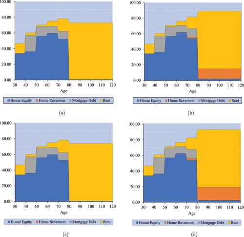
Figure 2. Average and percentiles of non-housing consumption (×$1,000 p.a.) over lifetime for cases A–D. Abbreviations: DA, Deferred annuities; HR, Home reversion; (+), available; (−), not available. (a) Case A: DA(−), HR(−) (b) Case B: DA(−), HR(+) (c) Case C: DA(+), HR(−) (d) Case D: DA(+), HR(+).

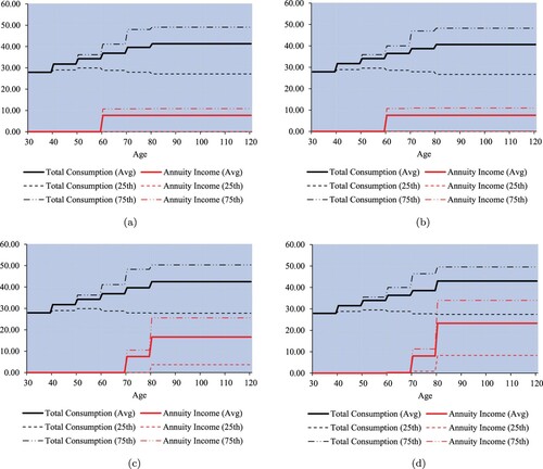
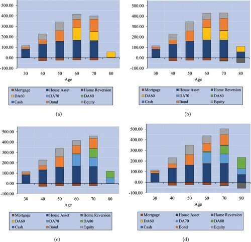
Figure 3. Average wealth composition (×$1,000) over lifetime in terms of financial assets, mortgage, home reversion, and annuities (DA60, DA70, DA80 start paying out at ages 60, 70, 80 resp.) for cases A–D. Abbreviations: DA, Deferred annuities; HR, Home reversion; (+), available; (−), not available. Time discretization means that cash flows are capitalized and occur in advance: see (18(18) $\begin{array}{rl}& {\mathbb{1}}_{\{n=n_0\}}{w}_0+L_n{\ddot{a}}_n(1-{\mathrm{{\rm Y}}}_L)+I_{A,n}{\ddot{a}}_n(1-{\mathrm{{\rm Y}}}_A)\\ & +X_{R,n}^{buy}{S}_{R,t}(1-{\phi }_R^u)+X_{HD,n}{S}_{H,n}(1-{\phi }_D^u)\\ & +\sum _{i\in \{C,B,E,HA\}}{X}_{i,n}^{sell}{S}_{i,n}(1-{\phi }_i^s)\\ & =C_n{\ddot{a}}_n+X_{HR,n}{S}_{H,n}{\phi }_{HR}^u{\ddot{a}}_n+D_{P,n}+D_{I,n}\\ & +\sum _{i\in \{C,B,E,HA,A(60),A(70),A(80\left)\right\}}{X}_{i,n}^{buy}{S}_{i,n}\left(1+{\phi }_i^u\right)\\ & +X_{HA,n}{S}_{H,n}{\phi }_{HA}^m{\ddot{b}}_n+{\mathbb{1}}_{\{n\in {\mathcal{N}}_{\mathcal{T}}\}}{S}_{W,n}{X}_{W,n}\end{array}$(18) ). Housing units are purchased at age 30 without a mortgage but with an initial wealth of $40k and a nominal 10-year loan against wages. (a) Case A: DA(−), HR(−) (b) Case B: DA(−), HR(+) (c) Case C: DA(+), HR(−) (d) Case D: DA(+), HR(+).

Result 1

Home reversion increases housing consumption in retirement, on average.

Result 1 follows from a comparison of the top two panels (top left and top right) of Figure 1. The top left panel (case A) precludes home reversion, whereas the top right panel (case B) does not. The amount of housing utilized (in terms of units of housing) increases by almost 30% in late retirement.² More housing units in this instance could mean better quality housing (through home improvements), or housing in a better or safer location. Home reversion generates a lump sum which can be used to fund consumption and enables the very elderly to stay in their house. Since mixed or shared ownership is possible, the individual can sell part of his property, through a shared ownership scheme, and pay rent on this using the lump sum obtained when he releases the remaining equity. The availability of deferred annuities does not appear to change this result materially: compare the top panels of Figure 1 with the bottom panels.

Result 2

Deferred annuities increase non-housing consumption in retirement, on average.

Compare the two left panels (top left and bottom left) of Figure 2. In the top left panel (case A), only the immediate annuity is available whereas deferred annuities are also available in the bottom left panel (case C). Average consumption increases by about 5% when deferred annuities are included. The 25th and 75th percentiles of consumption also increase. As from age 70, annuities provide just under half the retirement income when deferred annuities are available, compared to only about 20% when only the immediate annuity is available. Given the choice about annuitization timing, the investor prefers to annuitize later in case C than in case A. A home reversion contract, without deferred annuities, does not change average consumption significantly (compare the top left and top right panels of Figure 2) but a home reversion plan with access to deferred annuities enables the lump sum to be used to buy annuities at later ages (70 and 80) boosting late-age consumption (compare the top right and bottom right panels of Figure 2).³

Our results, in Figures 1 and 2, suggest that overall consumption does not fall in retirement, in line with classical results involving annuitization (Yaari 1965). However, Consumer Expenditure Survey data do show a dip in expenditure in retirement (Gourinchas and Parker 2002). In economics life-cycle studies, hump-shaped consumption with age is typically explained by hump-shaped and risky labour income (Cocco et al. 2005), whereas labour income is constant in our model. As pointed out by Fernandez-Villaverde and Krueger (2007), expenditure is not the same as consumption. A large asset may be bought around the time of retirement but it is consumed well into retirement.⁴ In practice, expenditure in retirement is affected by demographic changes (the death of a partner), family composition dynamics (children flying the nest) and health care needs (which are large towards the end of life), and none of these factors are considered in our model. Finally, home reversion products and deferred annuities were rare a decade or two ago, and are still relatively uncommon today, so the declining expenditure pattern of most retirees reflects this. It may be that our model describes normative behaviour—a stable level of consumption in retirement—that will become commonplace in the future if these products become more widely available.

Table 9 displays the average savings rate in the four different cases A–D. To define the savings rate, we first define the spending rate as the sum of non-housing consumption and rent (p.a.), expressed as a percentage of annual income (labour income before retirement, social security plus annuity income in retirement). The savings rate is then 100 minus the spending rate. In all four cases in Table 9, the average savings rate is high initially and generally declines with age, becoming negative in retirement as the individual dis-saves and spends from accumulated wealth. This mirrors the increasing profile of consumption with age which is observed in Figure 2. Comparing cases A and D in Table 9, the average savings rate is slightly higher at younger ages when deferred annuities and home reversion are available, but significantly less dis-saving occurs at the oldest ages as these products provide for retirement with built-in longevity protection.

Table 9. Average savings rate (%) over lifetime for cases A–D. Abbreviations: DA, Deferred annuities; HR, Home reversion; (+), available; (−), not available.

			Age
	DA	HR	30	40	50	60	70	80
Case A	−	−	25.45	19.38	13.71	−17.64	−27.36	−64.63
Case B	−	+	25.66	19.57	14.33	−16.55	−25.64	−59.19
Case C	+	−	25.44	19.37	13.70	−55.18	−28.03	−30.47
Case D	+	+	25.51	20.03	14.68	−50.73	−22.68	−7.87

Result 3

In retirement, equity allocation (as a proportion of financial assets) is higher on average in the presence of annuities and home reversion than in their absence.

In all four panels of Figure 3, the equity holding increases and then decreases with age. Cases A–D all allow immediate annuities, of course: see Table 8. To elucidate this further, Figure 4 shows the allocation to equities, as a proportion of financial assets, in the investment portfolio at different ages in cases C, D and E.

Figure 4. Average equity allocation (financial assets only) at different ages for cases C, D and E. Case E has neither home reversion nor annuity products. Case D has both home reversion and annuity products. Case C has annuities but not home reversion.

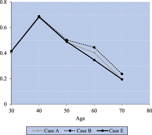
First, we note that equity allocation is hump-shaped in Figure 4. This result agrees empirically with household data (Cocco 2005). This is also consistent with the results of Horneff et al. (2010) and Koijen et al. (2011) who also include annuities, but not housing and home equity release products. Note that tax-deferred retirement plans are not included in our model. The presence of such plans may well tilt portfolios in favour of equity investment and away from home ownership initially, thereby flattening the hump-shaped equity profile at younger ages.⁵

In Figure 4, we observe a higher average allocation to equities at the later ages in case D (with annuities and home reversion) than in case E (without annuities and home reversion). Since income in retirement is more secure with annuity purchases and housing equity has been released in retirement, greater risky investment in equities is optimal in case D than in case E.

Case C (with annuities but without home reversion) is also shown in Figure 4. Comparing with case D (both annuities and home reversion), this shows that the release of home equity allows greater allocation of financial wealth to the stock market to take place later in life.

Result 4

Home ownership increases then decreases, renting decreases then increases, with age on average.

Result 4 is visible in all four panels of Figure 1, where home ownership is represented by mortgage plus personal housing equity. This result is also reproduced by Yao and Zhang (2005) and Kraft and Munk (2011), induced by the positive correlation between stochastic labour income and house prices in their model. A positive correlation means that, because of their large human capital, younger investors are already exposed to housing market risk, so they prefer to rent initially. In our model, labour income is deterministic but housing and equity returns are both risky. The initial rise in holding of housing parallels the rise in equity holding in that annuities provide secure income in retirement, so greater risk-taking is possible. Later, in retirement, liquidity is more constrained and selling existing property and renting accommodation means personal equity in housing can be released to smooth consumption inter-temporally.

6.4. Consumption, investment, and housing: without bequest

In the benchmark numerical example of section 6.1, with results described in section 6.3, there was a bequest motive ($\kappa =5$ in Table 6). A bequest motive is expected to reduce home reversion and annuitization because these products reduce wealth available to pass on. In this section, we consider a situation with no bequest motive ($\kappa =0$) and compare this with the earlier case with bequest ($\kappa =5$).

Result 5

A bequest motive initially depresses (non-housing) consumption and raises saving and investment, subsequently increasing wealth available to bequeathe, with little effect on home reversion and a small reduction in overall annuitization, on average.

The effect of a bequest motive is to reduce initial consumption on average, as may be observed by comparing the middle two panels of Figure 5. The middle left panel shows case D without bequest ($\kappa =0$), and the middle right panel shows case D with bequest ($\kappa =5$). Ultimate levels of average consumption are the same, with slightly higher amounts of income from annuities in the case without bequest.

Figure 5. Average number of housing units ($\times m^2$, top panels), average and percentiles of consumption (×$1,000 p.a., middle panels), and average wealth composition (×$1,000, bottom panels), without bequest ($\kappa =0$, left panels) and with bequest ($\kappa =5$, right panels), all for case D (with deferred annuities and home reversion).

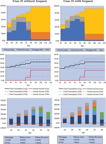
The higher lifetime savings are used to boost average investment in the housing, equity and bond market, as is evident from the bottom panels of Figure 5. About the same average amount of housing equity is released by means of home reversion at age 80 to buy an annuity in the two cases. The amounts of annuities held at ages 60 and 70 are lower with bequest than without, but about the same at age 80, on average. The bequest motive does not, on average, change the amount of housing consumed, as may be seen when comparing the top two panels of Figure 5, and there is less mortgage financing in the case with bequest.

This suggests that home reversion and deferred annuities retain their usefulness in supporting consumption in retirement, even in the presence of a bequest motive.

7. Discussion and concluding remarks

Annuities and home equity release products can provide individual investors with considerable freedom and choice to secure an optimal retirement income, yet they are rarely included in life-cycle models. We construct an optimal investment and consumption model with deferred and immediate annuities, with housing, mortgages, and home reversion products, and with the usual financial assets (cash, bond, equity).

We use multi-stage stochastic programming (MSP) to solve the optimization problem numerically. MSP allows us to integrate consistently models of a financial market, an annuity market, a housing market, and a home equity release product. MSP also allows for a solution in the presence of frictions such as transaction costs, taxes and management fees. Our first and principal contribution is therefore to obtain quantitative results that may be used in a practical lifetime investment setting and to show how MSP can be implemented.

We also show numerically that housing consumption in retirement may be greater when home reversion is available compared to when it is not. Likewise, non-housing consumption in retirement can be greater when deferred annuities are available compared to when they are not. The combination of these two products means that retirees can access their personal equity in their homes, without being forced to sell or leave their homes, and use the home reversion lump sum to buy annuities to secure their retirement income. Our model reproduces empirical features in household financial data. Equity allocation in overall wealth does not decline with age, as classical life-cycle models conclude, but instead increases and then decreases. Likewise, the young prefer renting to home ownership initially. Home ownership increases with age and then decreases past retirement, and vice-versa with renting. Finally, the presence of a bequest motive should prima facie depress the take-up of home equity release and annuitization. Our numerical results show that the bequest motive principally accelerates saving and investment at young and middle ages, resulting in greater wealth accumulation. Home reversion barely changes, and annuitization suffers only a mild reduction.

Although our model has a rich set of features and realistic constraints, it does have limitations and these must temper our conclusions. First, the timeline in our model is discretized coarsely, whereas in practice individuals can make consumption and investment decisions on an almost continuous basis. This is a limitation of MSP which will be ameliorated over time with ever-increasing computing power and newer techniques (Consiglio et al. 2016, Mulvey et al. 2020). Second, we have displayed average optimal solutions, but the solution is of course dynamic. Further work is required to determine how the solutions vary for different stochastic scenarios, e.g. combinations of low interest rates, high house prices and a falling stock market. Third, the optimal consumption and investment solution is likely to be sensitive to the parameters of the financial and housing market model, particularly the correlation coefficients. These are likely to change over different historical periods. Fourth, annuities are often shunned by investors who perceive them to be expensive because of loadings added to fair prices to cover insurers' costs, and because of longevity risk and low interest rates. Annuity loadings and longevity risk were ignored in our model. These issues relate to the so-called ‘annuity puzzle’ and deserve further investigation in our model. Another limitation of our study is that, in practice, investment also takes place within retirement plans, of either the defined contribution or defined benefit variety, with privileged tax treatment to encourage pension savings. It should be possible to include investment within separate pension vehicles in our model (Consiglio et al. 2015, Duarte et al. 2017). Direct property investment is highly undiversified in practice for most individuals and it is necessary to capture the idiosyncratic risk to which they are exposed. We have also used a stylized model with specific assumptions concerning, for example, the retirement age and labour income during working lifetime. The results should be tailored to individual circumstances in practice. Finally, regulatory and political risk is significant especially over the long term and we have not allowed for this. Tax rules and tax rates can change, especially after significant macroeconomic events such as the 2008 financial crisis or the 2020 Covid pandemic.

Further work to extend our model could proceed along several avenues. Inflation on prices, housing and wages should be included. A stochastic labour income, correlated to housing returns, is highly desirable. A flexible labour supply (number of hours worked) could be determined endogenously. In the real world, there are various types of annuities (inflation-indexed annuities and variable annuities) and other types of home equity release products (especially the reverse mortgage) that should be considered. Individuals must also contend with term life insurance, health insurance, and private pension plans, all of which may be significant products in their financial life-cycle. Finally, we assume that the risk preferences of individuals are described with a standard utility function exhibiting constant relative risk aversion (CRRA) but alternative objectives can be considered (Kim et al. 2020). These and other issues will be considered in future work.

Disclosure statement

No potential conflict of interest was reported by the author(s).

Notes

1 We assume throughout that units are perfectly divisible and fractional units can be held. No mixed-integer programming is therefore required.

2 Note that housing for one individual is displayed in Figure 1. For a household, this will typically be doubled.

3 It is worth emphasizing that the significant purchase of annuities which may be observed in Figure 2 is a function of the interest rate model in (1(1) $\text{d}{r}_t=\nu (\tilde{\theta }-r_t)\text{d}t+{\sigma }_0\text{d}{W}_{r,t},$(1) ) which governs annuity pricing. The interest rate model is parameterized as explained in section 6.1 but is not calibrated to today's yield curve where ultra-low interest rates prevail, making annuities expensive. The interest rate model is instead initialized at a stationary level capturing the historical average term structure of interest rates.

4 For example, many individuals buy a new car around the time of retirement, but consume services from this asset for many years into retirement. Others may buy a holiday cottage or cabin around the time of retirement, and then consume housing services from this asset thereafter. Although we do not model this here, an increase in consumption can occur at retirement particularly when individuals receive a tax-exempt lump-sum distribution from their pension plan.

5 Glide paths in target date funds, such as those of Vanguard (Daga et al. 2016), start at a higher level of equity allocation. They are designed for retirement plans whereas we consider a full life-cycle problem. Retirement plans benefit from a tax-advantaged status and do not usually hold residential housing assets.

6 The model can be reconfigured for use in practical situations as follows. Stages of increasing lengths, starting with 1 year, are used in the scenario tree. The model is then used as in receding horizon control where it is fully solved but only the investment and consumption decisions at the root node are carried out. The model is then solved again when the individual is one year older, with only the first step being implemented again, etc.

Appendices

Appendix 1.

Other optimization constraints

The main optimization constraints for the optimization problem in (14(14) $\begin{array}{rl}& \underset{{\mathcal{D}}_n,n\in \mathcal{N}}{max}\left[\sum _{t\in [0,\mathcal{T}]}\sum _{n\in {\mathcal{N}}_t}\left(\sum _{s=t}^{t+\mathrm{\Delta }t-1}\left[s\right]\delta e^{-\rho s}u\left(C_n^{1-\theta }{H}_n^{\theta }\right)\right){\mathbf{p}\mathbf{r}}_n\right.\\ & +\sum _{t\in [0,\mathcal{T})}\sum _{n\in {\mathcal{N}}_{t+\mathrm{\Delta }t}}\left[t\right]\delta \left[\mathrm{\Delta }t\right]\delta +t{e}^{-\rho (t+\mathrm{\Delta }t)}{\kappa }^{\gamma }u\left(W_n\right){\mathbf{p}\mathbf{r}}_n\\ & +\left.\sum _{s=\mathcal{T}}^{\tau -1}\sum _{n\in {\mathcal{N}}_{\mathcal{T}}}\left[s\right]\delta \left[\mathrm{\Delta }s\right]\delta +s{e}^{-\rho (s+\mathrm{\Delta }s)}{\kappa }^{\gamma }u\left(X_{W,n}\right){\mathbf{p}\mathbf{r}}_n\right],\end{array}$(14) ) are found in (15a(15a) $\begin{array}{rl}{H}_n& =X_{HA,n}+X_{HR,n},\end{array}$(15a) )–(21(21) $\begin{array}{rl}{W}_n& =\sum _{i\in \{C,B,E\}}{X}_{i,n^{-}}{S}_{i,n}\left(1-{\phi }_i^m\right)+\left(X_{HA,n^{-}}-X_{R,n^{-}}\right)S_{H,n}\\ & -\left(D_{H,n^{-}}+D_{I,n}\right).\end{array}$(21) ). Other constraints are required as follows: (A1) $\begin{array}{rl}{X}_{i,n},X_{i,n}^{buy},X_{i,n}^{sell}& \ge 0\mathrm{f}\mathrm{o}\mathrm{r}i\in \{C,B,E\}\mathrm{a}\mathrm{n}\mathrm{d}n\in \mathcal{N},\end{array}$(A1) (A2) $\begin{array}{rl}{X}_{i,n},X_{i,n}^{buy}& =0\mathrm{f}\mathrm{o}\mathrm{r}i\in \{C,B,E\}\mathrm{a}\mathrm{n}\mathrm{d}n\in {\mathcal{N}}_{\mathcal{T}},\end{array}$(A2) (A3) $\begin{array}{rl}{X}_{R,n}^{buy}& =0\mathrm{f}\mathrm{o}\mathrm{r}n\in \{{\mathcal{N}}_t,t\in [0,T\left)\right\},\end{array}$(A3) (A4) $\begin{array}{rl}{X}_{R,n}^{buy}& \ge 0\mathrm{f}\mathrm{o}\mathrm{r}n\in \{{\mathcal{N}}_t,t\in [T,\mathcal{T}\left]\right\},\end{array}$(A4) (A5) $\begin{array}{rl}{X}_{HA,n},X_{HA,n}^{buy},X_{HA,n}^{sell}& \ge 0\mathrm{f}\mathrm{o}\mathrm{r}n\in \mathcal{N},\end{array}$(A5) (A6) $\begin{array}{rl}{X}_{HR,n}& \ge 0\mathrm{f}\mathrm{o}\mathrm{r}n\in \mathcal{N},\end{array}$(A6) (A7) $\begin{array}{rl}{X}_{HD,n},D_{H,n}& \ge 0\mathrm{f}\mathrm{o}\mathrm{r}n\in \{{\mathcal{N}}_t,t\in [0,\mathcal{T}\left)\right\},\end{array}$(A7) (A8) $\begin{array}{rl}{X}_{HD,n},D_{H,n}& =0\mathrm{f}\mathrm{o}\mathrm{r}n\in {\mathcal{N}}_{\mathcal{T}},\end{array}$(A8) (A9) $\begin{array}{rl}{X}_{A\left(\psi \right),n}^{buy}& \ge 0\mathrm{f}\mathrm{o}\mathrm{r}\psi \in \{60,70,80\}\mathrm{a}\mathrm{n}\mathrm{d}\\ & n\in \{{\mathcal{N}}_t,t\in [T,\psi -\delta \left]\right\},\end{array}$(A9) (A10) $\begin{array}{rl}{X}_{A\left(\psi \right),n}^{buy}& =0\mathrm{f}\mathrm{o}\mathrm{r}\psi \in \{60,70\}\mathrm{a}\mathrm{n}\mathrm{d}\\ & n\in \{{\mathcal{N}}_t,t\in (\psi -\delta ,\mathcal{T}\left]\right\},\end{array}$(A10) (A11) $\begin{array}{rl}{X}_{W,n}& =0\mathrm{f}\mathrm{o}\mathrm{r}n\in \{{\mathcal{N}}_t,t\in [0,\mathcal{T}\left)\right\},\end{array}$(A11) (A12) $\begin{array}{rl}{X}_{W,n}& \ge 0\mathrm{f}\mathrm{o}\mathrm{r}n\in {\mathcal{N}}_{\mathcal{T}},\end{array}$(A12) (A13) $\begin{array}{rl}{W}_n,C_n,H_n& >0\mathrm{f}\mathrm{o}\mathrm{r}n\in \mathcal{N}.\end{array}$(A13) (A1(A1) $\begin{array}{rl}{X}_{i,n},X_{i,n}^{buy},X_{i,n}^{sell}& \ge 0\mathrm{f}\mathrm{o}\mathrm{r}i\in \{C,B,E\}\mathrm{a}\mathrm{n}\mathrm{d}n\in \mathcal{N},\end{array}$(A1) ) is a no-short sales constraint on financial assets. (A2(A2) $\begin{array}{rl}{X}_{i,n},X_{i,n}^{buy}& =0\mathrm{f}\mathrm{o}\mathrm{r}i\in \{C,B,E\}\mathrm{a}\mathrm{n}\mathrm{d}n\in {\mathcal{N}}_{\mathcal{T}},\end{array}$(A2) ) insists that financial assets are liquidated at the planning horizon $\mathcal{T}$. Home reversions can only be arranged during retirement and up to the planning horizon: (A3(A3) $\begin{array}{rl}{X}_{R,n}^{buy}& =0\mathrm{f}\mathrm{o}\mathrm{r}n\in \{{\mathcal{N}}_t,t\in [0,T\left)\right\},\end{array}$(A3) ) and (A4(A4) $\begin{array}{rl}{X}_{R,n}^{buy}& \ge 0\mathrm{f}\mathrm{o}\mathrm{r}n\in \{{\mathcal{N}}_t,t\in [T,\mathcal{T}\left]\right\},\end{array}$(A4) ). Housing cannot be shorted in (A5(A5) $\begin{array}{rl}{X}_{HA,n},X_{HA,n}^{buy},X_{HA,n}^{sell}& \ge 0\mathrm{f}\mathrm{o}\mathrm{r}n\in \mathcal{N},\end{array}$(A5) ), and cannot be rented out in (A6(A6) $\begin{array}{rl}{X}_{HR,n}& \ge 0\mathrm{f}\mathrm{o}\mathrm{r}n\in \mathcal{N},\end{array}$(A6) ). (A7(A7) $\begin{array}{rl}{X}_{HD,n},D_{H,n}& \ge 0\mathrm{f}\mathrm{o}\mathrm{r}n\in \{{\mathcal{N}}_t,t\in [0,\mathcal{T}\left)\right\},\end{array}$(A7) ) guarantees that mortgage debt and housing bought with mortgage are non-negative, while (A8(A8) $\begin{array}{rl}{X}_{HD,n},D_{H,n}& =0\mathrm{f}\mathrm{o}\mathrm{r}n\in {\mathcal{N}}_{\mathcal{T}},\end{array}$(A8) ) ensures that the mortgage is fully repaid by the planning horizon. (A9(A9) $\begin{array}{rl}{X}_{A\left(\psi \right),n}^{buy}& \ge 0\mathrm{f}\mathrm{o}\mathrm{r}\psi \in \{60,70,80\}\mathrm{a}\mathrm{n}\mathrm{d}\\ & n\in \{{\mathcal{N}}_t,t\in [T,\psi -\delta \left]\right\},\end{array}$(A9) ) and (A10(A10) $\begin{array}{rl}{X}_{A\left(\psi \right),n}^{buy}& =0\mathrm{f}\mathrm{o}\mathrm{r}\psi \in \{60,70\}\mathrm{a}\mathrm{n}\mathrm{d}\\ & n\in \{{\mathcal{N}}_t,t\in (\psi -\delta ,\mathcal{T}\left]\right\},\end{array}$(A10) ) state that annuities can only be bought at or before their first payment date. Life insurance is purchased only at the planning horizon: (A11(A11) $\begin{array}{rl}{X}_{W,n}& =0\mathrm{f}\mathrm{o}\mathrm{r}n\in \{{\mathcal{N}}_t,t\in [0,\mathcal{T}\left)\right\},\end{array}$(A11) ) and (A12(A12) $\begin{array}{rl}{X}_{W,n}& \ge 0\mathrm{f}\mathrm{o}\mathrm{r}n\in {\mathcal{N}}_{\mathcal{T}},\end{array}$(A12) ). Finally, (A13(A13) $\begin{array}{rl}{W}_n,C_n,H_n& >0\mathrm{f}\mathrm{o}\mathrm{r}n\in \mathcal{N}.\end{array}$(A13) ) is a non-negative wealth condition.

Note that, in our MSP model, mortgage interest payments are paid at the end of every time period: see (16b(16b) $\begin{array}{rl}{D}_{I,n}& ={\mathbb{1}}_{n\ne n_0}{D}_{H,n^{-}}\cdot (\exp \left(\left(r_{n^{-}}+\alpha \right)\mathrm{\Delta }t\right)-1).\end{array}$(16b) ). We disregard the individual's insolvency since negative overall wealth is not allowed in constraint (A13(A13) $\begin{array}{rl}{W}_n,C_n,H_n& >0\mathrm{f}\mathrm{o}\mathrm{r}n\in \mathcal{N}.\end{array}$(A13) ). Mortgage repayment is discretionary, as discussed in section 3.3, and $D_{P,n}$ is a decision variable in the optimization objective (14(14) $\begin{array}{rl}& \underset{{\mathcal{D}}_n,n\in \mathcal{N}}{max}\left[\sum _{t\in [0,\mathcal{T}]}\sum _{n\in {\mathcal{N}}_t}\left(\sum _{s=t}^{t+\mathrm{\Delta }t-1}\left[s\right]\delta e^{-\rho s}u\left(C_n^{1-\theta }{H}_n^{\theta }\right)\right){\mathbf{p}\mathbf{r}}_n\right.\\ & +\sum _{t\in [0,\mathcal{T})}\sum _{n\in {\mathcal{N}}_{t+\mathrm{\Delta }t}}\left[t\right]\delta \left[\mathrm{\Delta }t\right]\delta +t{e}^{-\rho (t+\mathrm{\Delta }t)}{\kappa }^{\gamma }u\left(W_n\right){\mathbf{p}\mathbf{r}}_n\\ & +\left.\sum _{s=\mathcal{T}}^{\tau -1}\sum _{n\in {\mathcal{N}}_{\mathcal{T}}}\left[s\right]\delta \left[\mathrm{\Delta }s\right]\delta +s{e}^{-\rho (s+\mathrm{\Delta }s)}{\kappa }^{\gamma }u\left(X_{W,n}\right){\mathbf{p}\mathbf{r}}_n\right],\end{array}$(14) ), but mortgage debt must be fully repaid by planning horizon $\mathcal{T}$, regarded as the maturity date of the mortgage: see (A8(A8) $\begin{array}{rl}{X}_{HD,n},D_{H,n}& =0\mathrm{f}\mathrm{o}\mathrm{r}n\in {\mathcal{N}}_{\mathcal{T}},\end{array}$(A8) ) above. This means that we can investigate the best way for the investor to pay off home loans. Although home reversion is irreversible, as enforced in (A4(A4) $\begin{array}{rl}{X}_{R,n}^{buy}& \ge 0\mathrm{f}\mathrm{o}\mathrm{r}n\in \{{\mathcal{N}}_t,t\in [T,\mathcal{T}\left]\right\},\end{array}$(A4) ), the individual can subsequently increase his housing equity by buying other housing units, which in practice may mean home improvements or house extensions.

Appendix 2.

Scenario generation for the Vasicek-GBMs model

Recall from section 5 that $\mathcal{N}$ is the set of all nodes in the scenario tree; ${\mathcal{N}}_t$ is the set of nodes at time t. The scenario tree consists of the nodes set $\{{\mathcal{N}}_t,t\in [0,\mathcal{T}\left]\right\}$. The set of children nodes of a node $n\in \{{\mathcal{N}}_t,t\in [0,\mathcal{T}\left)\right\}$ is denoted by $\left\{n^{+}\right\}$. Within the scenario tree, the time interval between node n and its children nodes $\left\{n^{+}\right\}$ is $\mathrm{\Delta }t$. Every node n has one unique parent node $n^{-}$, except the root node $n_0\in {\mathcal{N}}_0$.

At each node $n\in {\mathcal{N}}_t$, $R_{i,n}$ is the log-returns of an asset $i\in \{C,B,E,H\}$ over a $\mathrm{\Delta }t$-long time interval ending at time t ((4(4) $S_{i,t}=S_{i,t-\mathrm{\Delta }t}\cdot \exp \left(R_{i,t}\right),$(4) )). Accordingly, $R_{C,n}={\int }_{t-\mathrm{\Delta }t}^t{r}_s\text{d}s$ is the gross return of the cash fund; $R_{B,n}=a(M-\mathrm{\Delta }t)-a\left(M\right)-b(M-\mathrm{\Delta }t)r_n+b\left(M\right)r_{n^{-}}$ is the gross return of the bond fund ((5(5) $R_{B,t}=a(M-\mathrm{\Delta }t)-a\left(M\right)-b(M-\mathrm{\Delta }t)r_t+b\left(M\right)r_{t-\mathrm{\Delta }t},$(5) )); $R_{E,n}=\ln \left(S_{E,n}/S_{E,n^{-}}\right)$ is the gross return of the equity fund; and $R_{H,n}=\ln \left(S_{H,n}/S_{H,n^{-}}\right)$ is the gross return of the house price. $r_n$ is the Vasicek short rate observed at time t ((1(1) $\text{d}{r}_t=\nu (\tilde{\theta }-r_t)\text{d}t+{\sigma }_0\text{d}{W}_{r,t},$(1) )). Given the current short rate, the prices of annuity, whole-life immediate contract, and home reversion contract are determined by (6(6) $S_{A\left(\psi \right),t}=\sum _{m=\psi -\delta -t}^{\tau -t-1}{}_m{p}_{\delta +t}\exp \left(a\left(m\right)-b\left(m\right)r_t\right).$(6) ), (7(7) $S_{W,t}=\sum _{m=0}^{\tau -t-1}\left[m|\right]\delta +t\exp \left(a\left(m\right)-b\left(m\right)r_t\right).$(7) ), and (10(10) $\begin{array}{rl}{S}_{R,t}& =\sum _{m=0}^{\tau -t}\left(\left[m|\right]\delta +t-\left[m\right]\delta +t{\phi }_R^l\right)\exp \left(a\right(m)-b(m\left)r_t\right)\\ & \times \mathbb{E}\left[S_{H,t+m}\right|S_{H,t}].\end{array}$(10) ).

We generate the scenario tree by using the moment matching method (Høyland and Wallace 2001, Klaassen 2002). More precisely, we use the sequential approach of Høyland and Wallace (2001) with no-arbitrage constraints. A large multi-period scenario tree consists of many small single-period sub-trees. The first sub-tree has the limited number of outcomes corresponding to each child node in the set $\left\{n_0^{+}\right\}$. The outcomes of the first sub-tree are obtained by matching the first four moments of the conditional distributions of the four state variables $[r_{n_0^{+}}$, $R_{C,n_0^{+}}$, $R_{E,n_0^{+}}$, $R_{H,n_0^{+}}]$ on $r_{n_0}$. For the second-period sub-trees, the conditional outcomes are obtained by matching the four moments of the conditional distributions on the outcomes of the first sub-tree. The procedure is executed sequentially until the final-period sub-trees. By doing so, we ensure that all conditional properties are fully matched through the multi-period scenario tree.

At the root node $n_0$, the initial short rate $r_{n_0}$ is set to equal its mean level $\tilde{\theta }$ in Table 7. Each node n has six children nodes. The generated scenarios are arbitrage-free. This is achieved using the following procedure:

1. Given a node $n\in \mathcal{N}\setminus {\mathcal{N}}_{\mathcal{T}}$, generate scenarios for its children nodes $\left\{n^{+}\right\}$ by matching the four moments of conditional distributions of four state variables $[r_{n^{+}}$, $R_{C,n^{+}}$, $R_{E,n^{+}}$, $R_{H,n^{+}}]$ given the current short rate $r_n$.

2. Check if the generated scenarios preclude arbitrage opportunities (see Klaassen 2002). Go back to Step (i) if any arbitrage opportunity is found.

Step (ii) can be subsumed within Step (i).

The choice of 6 children nodes per parent node in the scenario tree satisfies both the moment matching conditions set out by Høyland and Wallace (2001) and general no-arbitrage conditions (there are 3 risky assets so that at least 4 children nodes are required to avoid arbitrage). We also divide up the timeline into regular stages to correspond to the regular financial reviews that an individual may have with an adviser during their financial life-cycle. Our consumption-investment solution then approximates, albeit coarsely, the optimal continuous-time intertemporal solution whilst avoiding the distortion that irregular time intervals would create.⁶

Since there are six children nodes for every non-terminal node and there are six stages (five periods), there are $6^5=7,776$ scenarios and $\sum _{j=0}^5{6}^j=9,331$ nodes. Generating each scenario tree takes about half an hour with Matlab by using a parallel loop parfor on an HP desktop computer with Intel CPU i7-7700 3.60 Ghz and 32 Gbyte memory. Optimization on the scenario tree is performed using the solver MOSEK, as described at the end of section 5. This is a fast and efficient solver and each instance of optimization takes only about $20\pm 5$ seconds on the same computer.

References

- Alai, D.H., Chen, H., Cho, D., Hanewald, K. and Sherris, M., Developing equity release markets: Risk analysis for reverse mortgages and home reversions. North Am. Actuarial J.; Schaumburg, 2014, 18, 217–241.
- Campbell, J.Y., Household finance. J. Finance, 2006, 61, 1553–1604.
- Case, B. and Quigley, J.M., The dynamics of real estate prices. Rev. Econ. Stat., 1991, 73, 50.
- Case, K.E. and Shiller, R.J., The efficiency of the market for single-family homes. Technical report, National Bureau of Economic Research. Cambridge, MA, USA, 1988.
- Chen, A., Haberman, S. and Thomas, S., An overview of international deferred annuity markets. SSRN Electron. J., 2019, 62, 2123–2167.
- Chen, H., Cox, S.H. and Wang, S.S., Is the home equity conversion mortgage in the united states sustainable? Evidence from pricing mortgage insurance premiums and non-recourse provisions using the conditional Esscher transform. Insurance: Math. Econ., 2010, 46, 371–384.
- Cho, D., Hanewald, K. and Sherris, M., Risk analysis for reverse mortgages with different payout designs. Asia-Pacific J. Risk Insurance, 2015, 9(1), 77–105.
- Cocco, J.F., Portfolio choice in the presence of housing. Rev. Financ. Stud., 2005, 18, 535–567.
- Cocco, J.F., Gomes, F.J. and Maenhout, P.J., Consumption and portfolio choice over the life cycle. Rev. Financ. Stud., 2005, 18, 491–533.
- Consigli, G., Iaquinta, G., Moriggia, V., Di Tria, M. and Musitelli, D., Retirement planning in individual asset–liability management. IMA J. Manage. Math., 2012, 23, 365–396.
- Consiglio, A., Carollo, A. and Zenios, S.A., A parsimonious model for generating arbitrage-free scenario trees. Quant. Finance, 2016, 16, 201–212.
- Consiglio, A., Tumminello, M. and Zenios, S.A., Designing and pricing guarantee options in defined contribution pension plans. Insurance: Math. Econ., 2015, 65, 267–279.
- Daga, A., Schlanger, T. and Westaway, P., Vanguard's approach to target retirement funds in the UK. Technical report, Vanguard, London, UK, 2016.
- Dempster, M., Asset liability management for individual households-abstract of the London discussion. British Actuarial J., 2011, 16, 441–467.
- Duarte, T.B., Valladao, D.M. and Veiga, A., Asset liability management for open pension schemes using multistage stochastic programming under Solvency-II-based regulatory constraints. Insurance: Math. Econ., 2017, 77, 177–188.
- Ezra, D., Most people need longevity insurance rather than an immediate annuity. Financial Anal. J., 2016, 72, 23–29.
- Federal Reserve Board, Survey of consumer finances. Technical Report, Federal Reserve, 2016.
- Fernandez-Villaverde, J. and Krueger, D., Consumption over the life cycle: Facts from consumer expenditure survey data. Rev. Econ. Statist., 2007, 89, 552–565.
- Flavin, M. and Yamashita, T., Owner-occupied housing and the composition of the household portfolio. Am. Econ. Rev., 2002, 92, 345–362.
- Gau, G.W., Efficient real estate markets: Paradox or paradigm?. Real Estate Econ., 1987, 15, 1–12.
- Gourinchas, P.O. and Parker, J.A., Consumption over the life cycle. Econometrica, 2002, 70, 47–89.
- Hanewald, K., Post, T. and Sherris, M., Portfolio choice in retirement-what is the optimal home equity release product? J. Risk Insurance, 2016, 83, 421–446.
- Horneff, W., Maurer, R. and Rogalla, R., Dynamic portfolio choice with deferred annuities. J. Bank. Finance, 2010, 34, 2652–2664.
- Høyland, K. and Wallace, S.W., Generating scenario trees for multistage decision problems. Manage. Sci., 2001, 47, 295–307.
- Huang, H., Milevsky, M.A. and Young, V.R., Optimal purchasing of deferred income annuities when payout yields are mean-reverting. Rev. Finance, 2016, 003.
- IFOA, S1PML/S1PFL all pensioners (excluding dependants), male/female lives. Technical Report, Institute and Faculty of Actuaries, 2019.
- Kim, W.C., Kwon, D.G., Lee, Y., Kim, J.H. and Lin, C., Personalized goal-based investing via multi-stage stochastic goal programming. Quant. Finance, 2020, 20, 515–526.
- Klaassen, P., Comment on ‘Generating scenario trees for multistage decision problems’. Manage. Sci., 2002, 48, 1512–1516.
- Koijen, R.S.J., Nijman, T.E. and Werker, B.J.M., Optimal annuity risk management. Rev. Finance, 2011, 15, 799–833.
- Konicz, A.K., Pisinger, D. and Weissensteiner, A., Optimal retirement planning with a focus on single and joint life annuities. Quant. Finance, 2016, 16, 275–295.
- Kraft, H. and Munk, C., Optimal housing, consumption, and investment decisions over the life cycle. Manage. Sci., 2011, 57, 1025–1041.
- Kraft, H., Munk, C. and Wagner, S., Housing habits and their implications for life-cycle consumption and investment. Rev. Finance, 2018, 22, 1737–1762.
- Maurer, R., Mitchell, O.S., Rogalla, R. and Kartashov, V., Lifecycle portfolio choice with systematic longevity risk and variable investment? Linked deferred annuities. J. Risk Insurance, 2013, 80, 649–676.
- Mayer, C.J. and Simons, K.V., Reverse mortgages and the liquidity of housing wealth. Real Estate Econ., 1994, 22, 235–255.
- Mulvey, J.M., Sun, Y., Wang, M. and Ye, J., Optimizing a portfolio of mean-reverting assets with transaction costs via a feedforward neural network. Quant. Finance, 2020, 20, 1239–1261.
- NRMLA, Industry statistics. Technical Report, National Reverse Mortgage Lenders Association, 2019.
- Scott, J.S., The longevity annuity: An annuity for everyone? Financial Anal. J., 2008, 64, 40–48.
- Shao, A.W., Hanewald, K. and Michael Sherris, A., House price models for banking and insurance applications: The impact of property characteristics. Asia-Pacific J. Risk Insurance, 2018, 12, 1–26.
- Shao, A.W., Hanewald, K. and Sherris, M., Reverse mortgage pricing and risk analysis allowing for idiosyncratic house price risk and longevity risk. Insurance: Math. Econ., 2015, 63, 76–90.
- Szymanoski, E.J., Risk and the home equity conversion mortgage. Real Estate Econ., 1994, 22, 347–366.
- Venti, S.F. and Wise, D.A., Aging and the income value of housing wealth. J. Public. Econ., 1991, 44, 371–397.
- Viceira, L.M., Optimal portfolio choice for long-horizon investors with nontradable labor income. J. Finance, 2001, 56, 433–470.
- Wang, L., Valdez, E.A. and Piggott, J., Securitization of longevity risk in reverse mortgages. North Am. Actuarial J.; Schaumburg, 2008, 12, 345–371.
- Weinrobe, M., An insurance plan to guarantee reverse mortgages: Abstract. J. Risk Insurance (1986–1998); Malvern, 1988, 55, 644.
- Yaari, M.E., Uncertain lifetime, life insurance, and the theory of the consumer. Rev. Econ. Stud., 1965, 32, 137–150.
- Yao, R. and Zhang, H.H., Optimal consumption and portfolio choices with risky housing and borrowing constraints. Rev. Financ. Stud., 2005, 18, 197–239.