
 ?Mathematical formulae have been encoded as MathML and are displayed in this HTML version using MathJax in order to improve their display. Uncheck the box to turn MathJax off. This feature requires Javascript. Click on a formula to zoom.
Abstract
In Friz et al. [Precise asymptotics for robust stochastic volatility models. Ann. Appl. Probab, 2021, 31(2), 896–940], we introduce a new methodology to analyze large classes of (classical and rough) stochastic volatility models, with special regard to short-time and small-noise formulae for option prices, using the framework [Bayer et al., A regularity structure for rough volatility. Math. Finance, 2020, 30(3), 782–832]. We investigate here the fine structure of this expansion in large deviations and moderate deviations regimes, together with consequences for implied volatility. We discuss computational aspects relevant for the practical application of these formulas. We specialize such expansions to prototypical rough volatility examples and discuss numerical evidence.
1. Introduction
In Friz et al. (Citation2021), precise short-time asymptotics were established for call and put option prices under stochastic volatility, under a set of abstract conditions satisfied by most classical and rough volatility (RoughVol) models. These results are refinements of large deviation statements, providing the higher-order, algebraic term in an asymptotic expression, known as Laplace expansion. For RoughVol models, short-dated large deviation pricing is due to Forde and Zhang (Citation2017), as is the induced implied volatility expansion (FZ expansion), which can be seen as a “rough” BBF (Berestycki–Busca–Florent Berestycki et al. Citation2004) formula. Our precise asymptotics provide a mechanism to compute refined implied volatility expansions, for log-strike , of the form
(1)
(1)
where the zero-order
term corresponds to the rough BBF formula in Forde and Zhang (Citation2017). The next-order term is seen of order
and hence increasingly important for small Hurst parameter H, the basic premise of RoughVol modeling. Inclusion of this term hinges on an accurate evaluation of a. In this paper, we assume that the volatility process is of the form
, where
is the Riemann–Liouville fractional Brownian motion (fBM) given by the self-similar Gaussian Volterra process in (EquationA3
(A3)
(A3) ). It has Hurst exponent
and it is ρ-correlated with the Brownian driving the asset.
The functions and
do not have explicit expressions and we discuss how to compute them numerically. Following Forde and Zhang (Citation2017),
can be computed using the Ritz method. Moreover, we propose a method for computing
based on a Karhunen–Loeve (KL) decomposition of the Brownian motions. (This entails a numerical approximation to an infinite-dimensional Carleman–Fredholm determinant.)
We also derive near-the-money (meaning, as ) expansions of
and of the term structure
which can alternatively be used for numerics (and have the advantage of being explicit functions of model parameters). From these asymptotics, we derive consequences for at-the-money (ATM) implied skew and curvature. We also refine some moderate deviation asymptotics for call prices and implied volatilities, cf. (Friz et al. Citation2017, Bayer et al. Citation2019, Gulisashvili Citation2020, Jacquier and Pannier Citation2020).
Being able to evaluate and
allows us to test the accuracy of the short-time asymptotics in practice. We do so with a numerical case study of the rough Bergomi (rBergomi) model. To exploit our general framework, we look at a volatility given by
(2)
(2)
so that for
we get the rBergomi model considered in Bayer et al. (Citation2016) and Bennedsen et al. (Citation2017) with constant forward variance, for
the rBergomi version in Bayer et al. (Citation2019) and Forde and Zhang (Citation2017). Note, however, that (Equation2
(2)
(2) ) is a genuine rBergomi model for any value of θ, as discussed in Remark 4.1. We compare our approximation to the FZ expansion from Forde and Zhang (Citation2017) and to the Edgeworth asymptotics in El Euch et al. (Citation2019). We consider how smiles vary as θ varies in (Equation2
(2)
(2) ) and as expiry t increases. We discuss and test the volatility term structure and its slope ATM, and observe how the term
improves the asymptotics as H decreases. We observe the same feature when we implement the moderate deviation asymptotics for implied volatility, where for H small the inclusion of the term structure correction
significantly improves on the numerical results presented in Bayer et al. (Citation2019).
Proofs rely on stochastic Taylor expansions, rate function representations in Forde and Zhang (Citation2017) and Bayer et al. (Citation2019) and on the local analysis on the Wiener space introduced in Friz et al. (Citation2021) and Bayer et al. (Citation2020). The classical Gao–Lee results (Gao and Lee Citation2014) are used to go from option prices to implied volatility asymptotics both in large and moderate deviation regimes.
Rough Volatility. It has been shown in recent years that RoughVol models provide great fits to observed volatility surfaces (Bayer et al. Citation2016) capturing fundamental stylized facts of implied volatility in a parsimonious way. Specifically, this class of models can reproduce the steep short end of the smile, displaying exploding implied skew (Alòs et al. Citation2007, Fukasawa Citation2011, Citation2017), and they are the only models consistent with the power law of the skew (Bayer et al. Citation2016, Lee Citation2005) not admitting arbitrage (Fukasawa Citation2021). RoughVol is also supported by statistical and time series analysis (Gatheral et al. Citation2018, Fukasawa et al. Citation2019, Bennedsen et al. Citation2021) and by market microstructure considerations (El Euch et al. Citation2018). Many authors have even argued that , such as to be consistent with a skew explosion close to
(Bayer et al. Citation2016, Citation2021). One main aspect of RoughVol is non-Markovianity. This is a serious complication when it comes to pricing, as Monte Carlo methods become more expensive and PDE methods are not available. For this reason, efficient simulation schemes have been proposed (Bayer et al. Citation2020, Bennedsen et al. Citation2017, McCrickerd and Pakkanen Citation2018). Fourier-based methods are available for the rough Heston model (El Euch and Rosenbaum Citation2019). Deep and machine learning approaches have also recently been discussed in Bayer et al. (Citation2019) and Goudenège et al. (Citation2020). Small maturity approximations are used in this context to obtain starting points for calibration procedures, which are then based on numerical evaluations.
Asymptotic option pricing. Classical motivation for (semi-closed form) asymptotic pricing includes fast calibration and a quantitative understanding of the impact of model parameters on relevant quantities such as implied skew and curvature/convexity along the moneyness dimension or slope along the term-structure dimension. Explicit expressions for such quantities (that follow in this setting from our expansion) and their shape characteristics are also used to choose the most appropriate model to be fitted to data (Ait-Sahalia et al. Citation2020), leave alone being the origin of some widely used parametrisations of the volatility surface. An interesting, if recent, addition to this list comes from a machine learning perspective: the form of an expansion such as (Equation1(1)
(1) ) may be viewed as expert knowledge, which significantly narrows the learning task to finer information such as the error in that expansions; it is equally conceivable to learn
and other components in the expansion.
Under Markovian stochastic volatility, expansion (Equation2(2)
(2) ) is analogous, e.g. to the result derived in Forde et al. (Citation2012) for the Heston model. There, the term structure is
(due to the diffusive scaling of the volatility), whereas here the correction term is
(due to the rough scaling of the volatility). Similar expansions are derived also in Osajima (Citation2015), for more general Markovian models, and (formally) in Medvedev and Scaillet (Citation2003) and Medvedev and Scaillet (Citation2007) for Markov stochastic volatility models with jumps.
In recent years several authors have studied the short-time behavior of RoughVol models. Theoretical results on short-time skew and curvature are given in Fukasawa (Citation2017) and Alòs and León (Citation2017). A second-order short-time expansion is given in El Euch et al. (Citation2019) for general (rough) stochastic volatility models. In Jacquier et al. (Citation2018), the pathwise large deviation behavior under rBergomi dynamics is studied. Pathwise large and moderate deviation principles for (possibly rough) Gaussian stochastic volatility models are established in Gulisashvili (Citation2020) and Gulisashvili (Citation2020), together with asymptotic results at the central limit (Edgeworth) regime. For the rough Heston model, the recent work (Forde et al. Citation2020) provides call expansions of the same type as ours, involving the energy function and the first-order algebraic term, at the same large deviations regime . (The rigid infinite-dimensional affine structure which underlies (Forde et al. Citation2020) is not available for rBergomi type models as considered in this work.) As already mentioned, our work builds on the large deviations principle proved in Forde and Zhang (Citation2017) for models with volatility
, and on Bayer et al. (Citation2019), where the at-the-money behavior of the Forde–Zhang rate function is used to prove moderate deviation principles and implied volatility asymptotics for the same type of models. The theoretical foundations of the present paper are given in Friz et al. (Citation2021).
In Section 2, we explain our RoughVol setting. In Section 3, we state and comment our results. In Section 4 we discuss and implement our results in the case of the rBergomi model. In Section 5, we show how Σ and a can be computed using Ritz method and KL decomposition. We collect all the proofs in Section 6.
2. Preliminaries on rough volatility
We consider the following RoughVol model, with , normalized to rate r = 0 and
(3)
(3)
where
are independent Brownian motions (BM) and
,
. We also write
. Moreover,
is a Gaussian Volterra process of the form
(4)
(4)
for a kernel
such that
is self-similar with exponent
, meaning
(5)
(5)
The BM W drives the stochastic “rough” volatility, meaning (with abusive notation) that
, where
is a smooth deterministic real-valued function. We denote
,
,
. We also denote
the spot volatility and
(6)
(6)
the derivatives of the volatility function at the initial condition. We consider a dependence in
in
, because this is the scaling of the variance of the fBm at time t. For this reason, this is the scaling of the time-dependent term in the rBergomi model, and also the scaling such that we observe a dependence in
in our precise asymptotics. We apply the abstract results proved in Friz et al. (Citation2021) for
. However, we expect these approximations to hold in greater generality: the same type of expansions should hold for other kernels such that
in (Equation4
(4)
(4) ) satisfies (Equation5
(5)
(5) ). Self-similarity is equivalent to the fact that K can be written in the following form
(7)
(7)
for a suitable function
(see Jost Citation2007, Lemma 2.4), so that all such kernels can be seen as a perturbation of
. Two classical processes of this form are the Mandelbrot–Van Ness and the Riemann–Liouville fBMs (see Appendix). Without loss of generality, we also assume
for t<s.
A similar setting has been considered in Forde and Zhang (Citation2017) and Bayer et al. (Citation2019). The main difference in the structure of the model is that here we allow for a direct dependence on time in , whereas in Forde and Zhang (Citation2017) and Bayer et al. (Citation2019) the volatility function depends only on the fBM, so
. As mentioned in the introduction, assuming that the volatility is a deterministic function only of the fBM rules out the rBergomi model
, see Bayer et al. (Citation2016) and Bennedsen et al. (Citation2017), from the analysis, so a modified version of rBergomi is considered in Bayer et al. (Citation2019). We discuss in detail both versions of this model in Section 4. With a volatility function
, one can write the dynamics of the log-price
as
(8)
(8)
In this case, a LDP holds, writing
, for
(9)
(9)
with speed
and rate function
(10)
(10)
where
and
is the Cameron–Martin norm. The existence of a minimizer above is obtained from a standard compactness argument. Through the space-time scaling
and the fact that, in law,
, this small-noise LDP translates to a short-time LDP. This result was proved for
in Forde and Zhang (Citation2017) and then extended to possible dependence in
in Friz et al. (Citation2021, Section 7.3). In general, when looking only at large (or moderate) deviations, the
-dependence in
does not affect the analysis, and the large (or moderate) deviations behavior is the same one would get with volatility
. In Friz et al. (Citation2021), we consider a general asymptotic setting, obtaining for generic stochastic volatility models (including RoughVol ones) precise asymptotics that refine such large deviations asymptotics. For such refinement, this
-dependence actually affects the asymptotics. In the present paper, we provide computationally relevant results that allow for the practical usage of such refined pricing asymptotics and discuss their consequences on the Black–Scholes implied volatility.
3. Results
We consider call and put prices under model (Equation8(8)
(8) ), i.e.
where k is the log-strike (or log-moneyness). In Friz et al. (Citation2021, Theorem 1.1) we obtain precise small-noise price expansions for generic (classical and rough) volatility dynamics. As in the classical Brownian case, such small-noise results can be translated into short-time results writing
. In this paper, we focus on the short-time setting. We write ∼ for asymptotic equivalence,
if
as
, and “≈” for “is close to” in informal terms. We also write
.
Assumption 3.1
Throughout the paper, we assume K in (Equation4(4)
(4) ) is of the form
In short-time, Friz et al. (Citation2021, Theorem 1.1) reads as follows:
Theorem 3.2
Let and
. Assume that a LDP holds for c, p above, and the existence of
moments for
. Then , for x>0 small enough, the rate function
is continuously differentiable at x and
for some function
with
as
. Similarly, for
close enough to 0, we have
for some function
with
as
. Moreover, such A can be expressed as
(11)
(11)
where
is a certain quadratic Wiener functional (specified in Friz et al. (Citation2021, Equation (7.4)), see also (Equation36
(36)
(36) ) below).
Remark 3.3
The fact that x>0 above has to be taken small enough is in order for the minimizer in (Equation10
(10)
(10) ) to be unique and non-degenerate. The latter means, in a nutshell, that the Hessian of
is strictly positive when restricted to those
such that
, and is equivalent to the finiteness of
defined above.
We write ,
and
for the inner product in
. We also denote
the adjoint of K in
so that
. Fully explicit expressions are computable in the case of the Riemann–Liouville fBM (Appendix) and in particular in the case of standard BM (this is the classical case of Markovian stochastic volatility). We denote
Lemma 3.4
Fine structure of A
For the following expansion holds for
as
(12)
(12)
As a consequence of Theorem 3.2 the following expansion holds for the Black–Scholes implied volatility (by a standard application of Gao and Lee (Citation2014), detailed in Friz et al. (Citation2021, Appendix D)).
Corollary 3.5
Asymptotic smile and term structure at the large deviations regime
Writing we have the following expansion, for
such that Theorem 3.2 holds:
(13)
(13)
where
(14)
(14)
and
(15)
(15)
Remark 3.6
In general, from a LDP for call prices follows the celebrated BBF formula for implied volatility (Berestycki–Busca–Florent Berestycki et al. Citation2004, see also Pham Pham Citation2010 for a derivation). Under RoughVol pricing with , this has been extended in Forde and Zhang (Citation2017) to
(16)
(16)
holding for fixed x, in short-time, with
. Thanks to the A-term in (Equation12
(12)
(12) ), we can extend this approximation, adding the term structure
. Note that the expansions hold for
, but for
their functional form is different, as some additional terms appear in
and in the term structure of the Black–Scholes implied volatility
.
We denote now
(17)
(17)
The short-time implied volatility coefficients in the previous statement can be expanded as follows near-the-money.
Theorem 3.7
At-the-money expansion of the coefficients
For the Σ coefficient has the following expansion:
(18)
(18)
where
The term structure coefficient, at the first order in x at 0, is
(19)
(19)
with
Remark 3.8
From definition (Equation14(14)
(14) )–(Equation15
(15)
(15) ) and from the fact that Λ is quadratic in x we see that (Equation19
(19)
(19) ) implies a relation between A and Λ for
.
Remark 3.9
Implied variance expansion (Equation13(13)
(13) ) reads as follows on implied volatility
(20)
(20)
In order to implement these expansions, one can use the methods discussed in Section 5, computing numerically the rate function
and
using FZ expansion, and then computing
using KL. However, this last step can be computationally expensive, since a large number of basis functions are needed for the KL decomposition to be accurate, for H close to 0. As an alternative, one can use approximation
(21)
(21)
for implied volatility, which follows from implied variance expansion (Equation13
(13)
(13) ) and (Equation19
(19)
(19) ). If the rate function cannot be computed, we can use (Equation18
(18)
(18) ) to expand the implied volatility as
(22)
(22)
In particular, we get the following explicit expansion for the ATM term structure:
(23)
(23)
Remark 3.10
The term structure of implied volatility
From the expansion of the ATM term structure (Equation23(23)
(23) ) we also see, in the short end, that
is increasing in t if
and decreasing if
. This may be compared with a large body of literature concerning monotonicity properties of the term structure of implied volatility, see e.g. (Camara et al. Citation2011, Guo et al. Citation2014, Krylova et al. Citation2009, Vasquez Citation2017).
Corollary 3.11
Skew and curvature at the large deviation regime
Let for
. Then, if
for
(24)
(24)
(25)
(25)
Remark 3.12
The quantities in the rhs of the equivalences converge as to
given in Theorem 3.7. The quantities in the lhs of the equivalences are finite difference approximations of ATM implied volatility skew
and curvature
. Such finite differences are relevant because only a finite number of prices are observable on real markets. They give skew and curvature at the large deviation regime, a result that complements (Fukasawa Citation2017, El Euch et al. Citation2019) (skew and curvature at central limit regime), Bayer et al. (Citation2019) (skew at moderate deviation regime), Forde et al. (Citation2020) (skew and curvature at large deviations regime for rough Heston), Alòs and León (Citation2017) (true skew and curvature).
From these formulas, we also infer the sign of implied skew and of implied curvature (convexity). Indeed, if , it is clear that
and that
(26)
(26)
Theorem 3.13
Moderate deviations
Assume that Λ is times continuously differentiable. Let
and
such that
. Set
. Then
Moreover
(27)
(27)
Remark 3.14
An implied volatility expansion similar to (Equation27(27)
(27) ) was proved in Bayer et al. (Citation2019), in the case
, for
, with remainder of order
. The derivatives of the rate function were computed until
, here we also computed
(cf. Lemma 6.1). This allows us to use the second-order moderate deviation (instead of first order as in Bayer et al. Citation2019)
Moreover, even if it does not show up in the asymptotics, the term structure can be incorporated as follows
and this provides a sensible improvement in the implementation of such short-time result (cf. figure ).
4. A case study: the rough Bergomi model
4.1. The rough Bergomi model
Introduced in Bayer et al. (Citation2016), as a modification of the classical Bergomi model where the exponential ( Ornstein–Uhlenbeck) kernel is replaced by a power-law kernel, the rBergomi model provides great fits of empirical implied volatility surfaces with a very small number of parametres. In such model, the volatility is given by the “Wick” exponential of a Riemann–Liouville fBM
(28)
(28)
In the most general framework (Bayer et al. Citation2016), the constant
is replaced by the forward variance curve, which is a function of time observable on the market (so it plays the role of an initial condition, cf. also Remark 4.1). The specific volatility in (Equation28
(28)
(28) ) did not fit in the framework of Forde and Zhang (Citation2017) and Bayer et al. (Citation2019), as in these papers the volatility is assumed to be
. For this reason, in Bayer et al. (Citation2019), the following version of the rBergomi model is considered
(29)
(29)
In this work we consider (Equation2
(2)
(2) ), a version of the rBergomi model with one additional parameter
, that includes both the previous ones (for
). The volatility function in (Equation3
(3)
(3) ) is
(30)
(30)
The interpretation of the parameters is the following:
is the spot volatility and η represents the volatility of volatility. The parameters of the driving noise are the Hurst exponent H of
and the correlation parameter ρ between the BM
driving the asset and W in (Equation4
(4)
(4) ). We can interpret the newly introduced θ parameter as a damping coefficient of the volatility.
Remark 4.1
Note that the forward variance curve model (and
filtration generated by W) induced by (Equation30
(30)
(30) ) and (Equation2
(2)
(2) ), is a genuine rBergomi model for any value of θ, with different values of θ corresponding to different specifications of the initial variance curve. More precisely, for fixed θ,
Coming now to short-time pricing, Lemma 6.1 holds for the general model in (Equation2(2)
(2) ), so that we are able to compare our asymptotics with large or moderate deviations results for the different versions of rBergomi in Bayer et al. (Citation2019), Forde and Zhang (Citation2017) and Jacquier et al. (Citation2018). However, in Corollary 3.5,
is not affected by the value of θ, but the term structure
is.
From the volatility function (Equation30(30)
(30) ) we get
so all constants can be simplified. In particular condition (Equation26
(26)
(26) ) for the convexity of the short-time smile (with
simplifies to
(note the dependence only on H, through K, and ρ). On calibrated parameters (for example in Bayer et al. Citation2016) we have that the condition for vanishing second derivative is almost satisfied. This means that the short-time ATM curvature is very close to 0, and indeed observed smiles are almost linear ATM.
All the constants in previous expansions depend on the kernel K. For the Riemann–Liouville kernel (EquationA4(A4)
(A4) ) the K-functionals involved are explicit, given in (EquationA5
(A5)
(A5) ).
4.2. Implementation of rough Bergomi
Our goal in this section is to compare expansion (Equation20(20)
(20) ) with other known implied volatility expansions under RoughVol. We consider:
Implied volatility from Monte Carlo pricing, using the hybrid scheme for rBergomi in Bennedsen et al. (Citation2017) with
(note that a slight modification of the implementation is necessary for
Our implied volatility expansion, where the term structure coefficient
The FZ expansion (Equation16
Expansion (Equation21
We first use the numerical methods detailed in next Section 5 to compute and
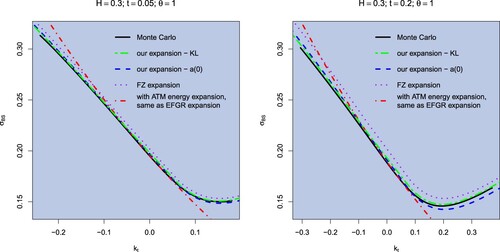
. In figure , we display implied volatility smiles in the rBergomi model with
, for varying t, where the rate function is computed using the Ritz method in Section 5.1 and the coefficient
is computed using the KL decomposition from Section 5.3. For comparison, we also use approximation
, and show (Equation21
(21)
(21) ). We notice that both implementations perform well, and the use of KL decomposition gives a better approximation of the right wing. On several simulations, this improvement of KL over expansion
is more evident when taking
, less when
.
Figure 1. Implied volatility smile approximations for the rBergomi model with parameters , for expiry
. The Monte Carlo price is computed via the hybrid scheme for rBergomi in Bennedsen et al. (Citation2017) with
, with
simulations and 500 time steps of length t/500. The rate function is computed using the Ritz method in Section 5.1 with N = 8 Haar basis functions, the coefficient
is computed using the Karhunen–Loeve decomposition with N = 300 Haar basis functions (KL). We also compare with
expanded at 0 (
).
Practically, implementation of the KL formula requires to approximate the infinite product (Equation38(38)
(38) ), and we observed that for smaller values of H the convergence of this product was much slower, requiring a prohibitively large number of basis functions, which is why we present these results for H = 0.3. We leave the numerically efficient implementation of the KL decomposition method for small values of H as a topic for future research. In what follows we will consider the approximation
, which is faster while still producing accurate smiles.
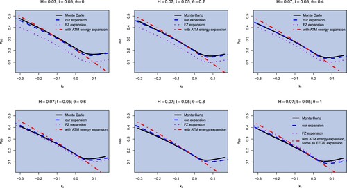
First, in figure , we show implied volatilities under model (Equation2(2)
(2) ), with realistic parameters (close to the calibrated parameter to the SPX volatility on February 4, 2010, see Bayer et al. Citation2016), varying θ from 0 to 1. We note how our approximation is general enough to be applicable for any θ, improving previous asymptotics in all cases. We also note a slight deterioration of the quality of the approximation in the right wing as
, that could be improved using KL to compute
.
Figure 2. Implied volatility smile approximation for the rBergomi model with parameters , for expiry t = 0.05. The Monte Carlo price is computed via the hybrid scheme for rBergomi in Bennedsen et al. (Citation2017) with
, with
simulations and 500 time steps. The rate function is computed using the Ritz method with N = 9 Fourier basis functions.
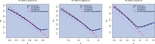
Then, instead of varying θ, we fix and show in figure the comparison with the same approximations as before, when the expiry t increases. We see how our expansion lifts the FZ expansion, improving the approximation of the Monte Carlo price. The difference between the two approximations is due to the term structure correction
. Clearly, the effect of this correction becomes more evident as t increases. On a number of numerical experiments, it is also clear that this correction becomes more and more important as
, not surprisingly since
is larger, for small t, when H vanishes.
Figure 3. Implied volatility smile approximation for the rBergomi model with parameters , for expiry t = 0.01, 0.05, 0.2. The Monte Carlo price is computed via the hybrid scheme for rBergomi in Bennedsen et al. (Citation2017) with
, with
simulations and 500 time steps of length t/500. The rate function is computed using the Ritz method with N = 9 Fourier basis functions.
Now we check how our approximations behave as time increases. To do so, in figure , we show the ATM term structure of implied volatility, comparing ATM implied volatilities computed using Monte Carlo simulations and expansion (Equation23(23)
(23) ), for rBergomi with
and
. We do so for parameters as in figures and , with H = 0.3, and for a different choice of parameters with H = 0.1 and a smaller volatility of volatility η, as in Bayer et al. (Citation2019, Section 4). The value of η and H affect the quality of the approximation, which is less accurate for H very close to 0 and
. On the other hand, as we show in figure , for H = 0.3 and
or H very close to 0 and
the short-time approximation is very good. This is consistent with the considerations on the interplay of H and η in El Euch et al. (Citation2019, Page 505). We also see how the term structure is increasing in case
and decreasing in case
. This is always the case:
in (Equation19
(19)
(19) ) is always positive for
, always negative for
(cf. Remark 3.10). Also note that if the coefficient
were taken non-constant, the slope of the term structure would also be affected.
Figure 4. Term structure of volatility for the rBergomi model with parameters (above) and with parameters
(below). We plot ATM implied volatility as expiration time increases. We consider shorter expiries in the case of rougher trajectories (smaller Hurst parameter H; however, in this case we also take a smaller vol-of-vol parameter η). The Monte Carlo prices are computed via the hybrid scheme in Bennedsen et al. (Citation2017) with
, with
simulations and 500 time steps.
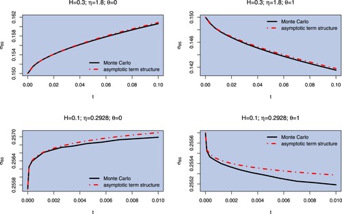
Figure 5. Moderate deviation with and x = 0.4 (time varying log-strike
) of implied volatility in rBergomi model with
. Simulation parameters:
simulation paths, 500 time steps. Time interval
.
![Figure 5. Moderate deviation with β=0.06 and x = 0.4 (time varying log-strike kt=xt1/2−H+β) of implied volatility in rBergomi model with σ0=0.2557,η=0.2928,ρ=−0.7571,H=0.1,θ=0. Simulation parameters: 108 simulation paths, 500 time steps. Time interval [0,0.1].](/cms/asset/e2b55de1-c477-46ef-8d90-ac58bddeb7ee/rquf_a_1999486_f0005_oc.jpg)
Finally, as in Remark 3.14, we consider moderate deviations. Figure is as in Bayer et al. (Citation2019, Figure ), the “very rough” case H = 0.1 (which was the most problematic case in Bayer et al. (Citation2019)). We are plotting, with , where
, the Monte Carlo implied volatility and its approximation
considering terms up to the first order moderate deviation
, then up to the second-order moderate deviation
, and finally considering also the term structure
. We see how the term structure term improves the moderate deviation pricing. This also explains why, in Bayer et al. (Citation2019), the moderate deviation pricing gets worse as
, since the distance of such price from the real (Monte Carlo) one is of order
. We also see that using the second order moderate deviation actually does not improve much, and this follows from the fact that the curvature is almost 0 with such choice of parameters (cf. Remark 3.14). As for the term structure, the accuracy of the approximation formula based on moderate deviations gets worse as η increases, for fixed H.
Remark 4.2
As mentioned above, Monte Carlo pricing is implemented using the hybrid scheme, which introduces a bias in the volatility process, while this process could be simulated exactly. However, in extensive simulations we find that the exact simulation scheme is more unstable for very short maturities, even with a trajectories and 500 time steps. This is most likely due to the singularity of the kernel at 0, which is what the hybrid scheme takes care of. On the other hand, with such a large number of paths and fine discretisation, for larger maturities the two schemes display no visible difference. Following these considerations, we used for our figures Monte Carlo prices simulated via the hybrid scheme in Bennedsen et al. (Citation2017).
Remark 4.3
In Forde and Zhang (Citation2017, Section 4.5) asymptotics for model (Equation3(3)
(3) ) with volatility driven by a Mandelbrot–Van Ness fBm (EquationA2
(A2)
(A2) ) are implemented. Without being completely rigorous, we have applied our expansion also in this case. We computed the K-functional numerically, as in this case no explicit formulas are available. Also in this case the term
lifts the smile, which gets closer to the real (Monte Carlo) implied volatility, for small
, with respect to the sole FZ expansion.
5. Computing the coefficients via projections
5.1. Computing using the Ritz method
In order to use (Equation20(20)
(20) ), the first challenge is the computation of the rate function. A numerical approximation to Λ can be obtained as described in Gelfand and Fomin (Citation2000, Section 40), using the Ritz method, as is done in Forde and Zhang (Citation2017). Natural choices for the orthonormal basis (ONB)
of
are the Fourier basis,
(31)
(31)
or the Haar basis,
(32)
(32)
We consider functions
with
so that
for
fixed. Then we minimize
with
(33)
(33)
over the Fourier coefficients
. This representation of the energy function is also taken from Forde and Zhang (Citation2017) (see notation in Bayer et al. Citation2019, Proposition 5.1). The minimizing value for
is therefore our approximation for the energy and the corresponding function
is the approximate most likely path for the fBm
associated with final condition x.
5.2. A stochastic Taylor development
The following stochastic Taylor expansion is sketched in Friz et al. (Citation2021, Section 7.2) for . As discussed in Section 2 and Friz et al. (Citation2021, Section 7.3), our expansions can actually be carried out in the more general setting
. Under such volatility dynamics, the (rescaled) log-price process is as in (Equation9
(9)
(9) ). As in Friz et al. (Citation2021, Section 7.2), we can shift the dynamics via
, and apply Girsanov theorem in order to center Brownian fluctuations in the minimizer. Then, a stochastic Taylor expansion gives
where
is smallFootnote1 , with
(34)
(34)
(cf. Friz et al. Citation2021, Section 7.2) and
(35)
(35)
The following formula for
follows as Friz et al. Citation2021, Equation 7.5
(36)
(36)
where we write
and
5.3. Computing using Karhunen–Loeve decomposition
Assume we are given computed by the Ritz method. Note then that
is obtained from
via the following formula
(37)
(37)
with
as in (Equation33
(33)
(33) ), as can be seen by optimizing over
for fixed h in the definition (Equation10
(10)
(10) ) of the rate function. Then we assume a Karhunen–Loeve (KL) decomposition of
:
where
is the ONB in (Equation31
(31)
(31) ) or (Equation32
(32)
(32) ) and
are i.i.d. standard Gaussians. This implies
with
. This yields
where
In particular
Note then that
We then can write all the terms in
as follows. We denote
and
. Now, expanding (Equation36
(36)
(36) ) with some long but standard computations we get to
where
and
Recall that one has
where
and since
is an element of the homogeneous Wiener chaos of order 2, the expectation above can be computed as the Carleman–Fredholm determinant
, where M is the symmetric matrix
Namely one has
(38)
(38)
where
are the eigenvalues of M (note that the fact that all
comes from the non-degeneracy assumption). This formula is a simple integral computation if M is diagonal, and the general case follows by diagonalization, cf e.g. Inahama (Citation2013, Remark 5.5) or Janson (Citation1997, p.78).
Of course, in practice we consider approximations ,
obtained by truncating the sums to only keep indices
, where N is fixed, so that all the sums above are then replaced by finite sums. One also needs to compute numerically the integrals appearing in the definition of the coefficients
, α, β. We have found the Haar basis to be more convenient than the Fourier basis for this purpose since the
's have explicit expressions in that case.
6. Proofs
6.1. Energy expansion
Lemma 6.1
Fourth order energy expansion
Consider a stochastic volatility model following dynamics (Equation3(3)
(3) ) and the associated energy function in (Equation10
(10)
(10) ). Let
be the energy function in (Equation10
(10)
(10) ). Then
where
(39)
(39)
and
Remark 6.2
In this lemma we expand the rate function , which has been studied first in Forde and Zhang (Citation2017). The second- and third-order terms in (Equation39
(39)
(39) ) have been computed in Bayer et al. (Citation2019, Theorem 3.4). In both these papers, the volatility function is supposed to be
, but adding the dependence
does not change the large deviations behavior, meaning that the rate function is the same as the one of the model given by
.
Proof.
We have the following development for the minimizer in (Equation10
(10)
(10) ), for
:
(40)
(40)
with
where
have been also computed in Bayer et al. (Citation2019). We make here the ansatz that the expansion goes on one more order with γ, that we do not actually need to compute. The existence of such γ follows from the smoothness of
(cf. Friz et al. Citation2021 and Bayer et al. Citation2019, Section 5.2). We can compute, using
and
,
We also have
(41)
(41)
We use now (Equation33
(33)
(33) ) and compute
(42)
(42)
from which we get
We also have, from (Equation40
(40)
(40) )
Now we write, from Bayer et al. (Citation2019, Proposition 5.1),
and use the expansions above for the two summands. The fourth-order expansion of
follows.
6.2. Proof of Lemma 3.4
Let us take .
STEP 1: We first need to expand in (Equation10
(10)
(10) ), for small x (an expansion of
was computed in Bayer et al. Citation2019). We write
(43)
(43)
for the Itô map associated with the RoughVol model (Equation8
(8)
(8) ). Computing the Frechet derivative of
with respect to the second component at
in the direction f we get (cf. (Equation34
(34)
(34) ))
(44)
(44)
From the first order optimality condition (Friz et al. Citation2021, Appendix B), we get that for
minimizer and any
in the Cameron–Martin space
,
Let f be the second component of
. Using (Equation44
(44)
(44) ) we get
Now, from (Equation39
(39)
(39) ) we derive that, for
,
(45)
(45)
We get
We also have
(46)
(46)
and
STEP 2: We recall here, from Friz et al. (Citation2021), the definition of some quantities needed to compute
. Let
be as in (Equation34
(34)
(34) ) and let us write
for its variance. We recall, again from Friz et al. (Citation2021, Equation (6.3)),
, from which we get
(47)
(47)
From (Equation34
(34)
(34) ) we define and compute
(48)
(48)
(Note that
are in the Cameron–Martin space). From (Equation11
(11)
(11) ) we have that
in Theorem 3.2 is
where
is given in (Equation36
(36)
(36) ).
STEP 3: We can expand now such quantity, for and we get
(49)
(49)
where
denotes
. The statement of the theorem follows from the computation of the quantities in (Equation49
(49)
(49) ).
STEP 4: We compute
and we obtain, also using (Equation48
(48)
(48) ),
(50)
(50)
where we have used
We have
Putting together the previous expressions and using
and
we get
(51)
(51)
This implies, together with (Equation47
(47)
(47) ),
(52)
(52)
We can now compute
where
so that
We also compute
and all these quantities can be expanded in x using (Equation51
(51)
(51) ). Now we use (Equation36
(36)
(36) ) to write, in the case
(53)
(53)
Moreover, using (Equation46
(46)
(46) ),
Now, also using (Equation36
(36)
(36) ) and (Equation51
(51)
(51) ) we get
STEP 5: We need now to compute
where (using definitions and (Equation50
(50)
(50) ))
We can rewrite
and, differentiating the product
with
independent of B. Therefore, by Itô isometry,
We can apply again Itô isometry to compute the last expectations, and
At this point it is a (long) calculus excercise (noting
) to show that
(54)
(54)
STEP 6: Substituting in (Equation49(49)
(49) ) we get
and we get Theorem Equation12(12)
(12) .
STEP 7: When ,
in (Equation36
(36)
(36) ) has an additional summand. Let us write
so that
has the same expression as
in the rough case
. For
we can write
(55)
(55)
so that
(56)
(56)
and, using (Equation41
(41)
(41) )
(57)
(57)
Now,
in Theorem 3.2 is
with
as above. Expanding in x we find
(58)
(58)
(we have used (Equation39
(39)
(39) ) and (Equation53
(53)
(53) )).
6.3. Proof of Theorem 3.7
A Taylor expansion gives
The explicit expressions for the three terms now follow from Lemma 6.1. Let us compute
. The rate function is quadratic and
. Then, using Taylor developments of Λ and
we get
From Lemma 6.1,
and, with
given in Lemma Equation12
(12)
(12) , we have when
with
with
defined in (Equation17
(17)
(17) ). Now, as a consequence of Lemma 6.1, we have
and the expansion of
follows. When
,
with
We conclude as in the case
.
6.4. Proof of Theorem 3.13
The call asymptotics is a corollary of Theorem 3.2, taking into consideration that
and that
under
. Recall
and the first statement follows.
Let us write ,
,
and
. We intend to apply (Gao and Lee Citation2014, Corollary 7.1, Equation (7.2)), where
denotes
and V denotes
. To do so, we notice that
(59)
(59)
when
and
. In the notation of Gao and Lee (Citation2014), we have
and G will be computed for
, so let us compute
and take care of the logarithmic terms in t. For
,
So
(60)
(60)
Equations (Equation59
(59)
(59) ) and (Equation60
(60)
(60) ) tell us that
(61)
(61)
The proof now boils down to writing the development of this factor using the Taylor developement of
, with
. We have, for
,
using
for
. Also notice
because
. We have
(62)
(62)
So from (Equation61
(61)
(61) ) and (Equation62
(62)
(62) )
(63)
(63)
We apply now (Gao and Lee Citation2014, Corollary 7.1, Equation (7.2)):
and obtain expansion (Equation27
(27)
(27) ).
Acknowledgments
We are grateful to C. Bayer and M. Fukasawa for discussion and to F. Bourgey and M. Pakkanen for the Python and R code for simulating the rough Bergomi model. We thank an anonymous reviewer for several remarks that helped us to improve the paper.
Disclosure statement
No potential conflict of interest was reported by the author(s).
Correction Statement
This article has been corrected with minor changes. These changes do not impact the academic content of the article.
Additional information
Funding
Notes
1 The precise control of this remainder is detailed in Friz et al. (Citation2021) and requires the sophisticated mathematical framework of regularity structures, that we do not intend to introduce in this paper. The interested reader is referred to Bayer et al. (Citation2020) and Friz et al. (Citation2021).
References
- Ait-Sahalia, Y., Li, C. and Li, C.X., Implied stochastic volatility models. Rev. Financ. Stud., 2020, 34, 394–450.
- Alòs, E. and León, J., On the curvature of the smile in stochastic volatility models. SIAM J. Financ. Math., 2017, 8(1), 373–399.
- Alòs, E., León, J. and Vives, J., On the short-time behavior of the implied volatility for jump-diffusion models with stochastic volatility. Finance Stoch., 2007, 11(4), 571–589.
- Bayer, C., Friz, P. and Gatheral, J., Pricing under rough volatility. Q. Finance, 2016, 16(6), 887–904.
- Bayer, C., Friz, P.K., Gassiat, P., Martin, J. and Stemper, B., A regularity structure for rough volatility. Math. Finance, 2020, 30(3), 782–832.
- Bayer, C., Friz, P.K., Gulisashvili, A., Horvath, B. and Stemper, B., Short-time near-the-money skew in rough fractional volatility models. Quant. Finance, 2019, 19(5), 779–798.
- Bayer, C., Hammouda, C.B. and Tempone, R., Hierarchical adaptive sparse grids and quasi-Monte Carlo for option pricing under the rough Bergomi model. Quant. Finance, 2020, 20(9), 1457–1473.
- Bayer, C., Harang, F.A. and Pigato, P., Log-modulated rough stochastic volatility models. SIAM J. Financ. Math., 2021, 12(3), 1257–1284.
- Bayer, C., Horvath, B., Muguruza, A., Stemper, B. and Tomas, M., On deep calibration of (rough) stochastic volatility models. arXiv preprint arXiv:1908.08806, 2019,
- Bennedsen, M., Lunde, A. and Pakkanen, M.S., Hybrid scheme for Brownian semistationary processes. Finance Stoch., 2017, 21(4), 931–965.
- Bennedsen, M., Lunde, A. and Pakkanen, M.S., Decoupling the short- and long-term behavior of stochastic volatility. J. Financ. Econ., 2021, nbaa049.
- Berestycki, H., Busca, J. and Florent, I., Computing the implied volatility in stochastic volatility models. Commun. Pure. Appl. Math., 2004, 57(10), 1352–1373.
- Camara, A., Krehbiel, T. and Lib, W., Expected returns, risk premia, and volatility surfaces implicit in option market prices. J. Banking Finance, 2011, 35(1), 215–230.
- El Euch, O., Fukasawa, M., Gatheral, J. and Rosenbaum, M., Short-term at-the-money asymptotics under stochastic volatility models. SIAM J. Financ. Math., 2019, 10(2), 491–511.
- El Euch, O., Fukasawa, M. and Rosenbaum, M., The microstructural foundations of leverage effect and rough volatility. Finance Stoch., 2018, 22(2), 241–280.
- El Euch, O. and Rosenbaum, M., The characteristic function of rough heston models. Math. Finance, 2019, 29(1), 3–38.
- Forde, M., Gerhold, S. and Smith, B., Small-time, large-time and H→0 asymptotics for the rough heston model. Math. Finance, 2020.
- Forde, M., Jacquier, A. and Lee, R., The small-time smile and term structure of implied volatility under the Heston model. SIAM J. Financ. Math., 2012, 3(1), 690–708.
- Forde, M. and Zhang, H., Asymptotics for rough stochastic volatility models. SIAM J. Financ. Math., 2017, 8(1), 114–145.
- Friz, P.K., Gassiat, P. and Pigato, P., Precise asymptotics: Robust stochastic volatility models. Ann. Appl. Probab., 2021, 31(2), 896–940.
- Friz, P.K., Gerhold, S. and Pinter, A., Option pricing in the moderate deviations regime. Math. Finance, 2017, 28(3), 962–988.
- Fukasawa, M., Asymptotic analysis for stochastic volatility: Martingale expansion. Finance Stoch., 2011, 15(4), 635–654.
- Fukasawa, M., Short-time at-the-money skew and rough fractional volatility. Quant. Finance, 2017, 17(2), 189–198.
- Fukasawa, M., Volatility has to be rough. Quant. Finance, 2021, 21(1), 1–8.
- Fukasawa, M., Takabatake, T. and Westphal, R., Is volatility rough? arXiv preprint arXiv:1905.04852, 2019.
- Gao, K. and Lee, R., Asymptotics of implied volatility to arbitrary order. Finance Stoch., 2014, 18(2), 349–392.
- Gatheral, J., Jaisson, T. and Rosenbaum, M., Volatility is rough. Quant. Finance, 2018, 18, 1–17.
- Gelfand, I.M. and Fomin, S.V., Calculus of Variations, 2000 (Dover Publications: Englewood Cliffs, NJ).
- Goudenège, L., Molent, A. and Zanette, A., Machine learning for pricing American options in high-dimensional Markovian and non-Markovian models. Quant. Finance, 2020, 20(4), 573–591.
- Gulisashvili, A., Gaussian stochastic volatility models: Scaling regimes, large deviations, and moment explosions. Stoch. Proc. Appl., 2020, 130(6), 3648–3686.
- Gulisashvili, A., Time-inhomogeneous Gaussian stochastic volatility models: Large deviations and super roughness. arXiv preprint arXiv:2002.05143, 2020.
- Guo, B., Han, Q. and Zhao, B., The Nelson-Siegel model of the term structure of option implied volatility and volatility components. J. Futures Mark., 2014, 34(8), 788–806.
- Inahama, Y., Laplace approximation for rough differential equation driven by fractional Brownian motion. Ann. Probab., 2013, 41(1), 170–205.
- Jacquier, A., Pakkanen, M.S. and Stone, H., Pathwise large deviations for the rough Bergomi model. J. Appl. Probab., 2018, 55(4), 1078–1092.
- Jacquier, A. and Pannier, A., Large and moderate deviations for stochastic Volterra systems. arXiv preprint arXiv:2004.10571, 2020.
- Janson, S., Gaussian Hilbert Spaces, Vol. 129, 1997 (Cambridge University Press).
- Jost, C., A note on ergodic transformations of self-similar Volterra Gaussian processes. Electron. Commun. Probab., 2007, 12, 259–266.
- Krylova, E., Nikkinen, J. and Vähämaa, S., Cross-dynamics of volatility term structures implied by foreign exchange options. J. Econ. Bus., Sept. 2009, 61(5), 355–375.
- Lee, R.W., Implied volatility: Statics, dynamics, and probabilistic interpretation. In Recent Advances in Applied Probability, pp. 241–268, 2005 (Springer: New York).
- Mandelbrot, B. and Van Ness, J.W., Fractional Brownian motions, fractional noises and applications. SIAM Rev., 1968, 10, 422–437.
- McCrickerd, R. and Pakkanen, M.S., Turbocharging Monte Carlo pricing for the rough bergomi model. Quant. Finance, 2018, 18(11), 1877–1886.
- Medvedev, A. and Scaillet, O., A simple calibration procedure of stochastic volatility models with jumps by short term asymptotics. Research Paper No. 93, September 2003, FAME – International Center for Financial Asset Management and Engineering, 2003. Available at SSRN 477441, 2003.
- Medvedev, A. and Scaillet, O., Approximation and calibration of short-term implied volatilities under jump-diffusion stochastic volatility. Rev. Financ. Studies, 2007, 20(2), 427–459.
- Nualart, D., The Malliavin Calculus and Related Topics, Vol. 1995, 2006 (Springer).
- Osajima, Y., General asymptotics of Wiener functionals and application to implied volatilities. In Large Deviations and Asymptotic Methods in Finance, pp. 137–173, 2015 (Springer).
- Pham, H., Large deviations in finance. Third SMAI European Summer School in Financial Mathematics, 2010.
- Vasquez, A., Equity volatility term structures and the cross section of option returns. J. Financ. Quant. Anal., 2017, 52(06), 2727–2754.
Appendix: Fractional Brownian motion
The fBM is a “rough” continuous-time Gaussian process in that, depending on a parameter , its trajectories are locally Hölder continuous of any order strictly less than H. Unlike classical BM, the increments of fBm are not independent if
. The fBM was introduced for the first time by Mandelbrot and Van Ness in Mandelbrot and Van Ness (Citation1968) as the following stochastic integral, for
:
where Z is a BM and
. Such process is Gaussian with covariance
(A1)
(A1)
It can also be represented as a Volterra integral on the interval
:
(A2)
(A2)
with
as in Nualart (Citation2006) or Forde and Zhang (Citation2017, Section 3.1)). One can consider the following variant of fBM, known as Riemann–Liouville process (Mandelbrot and Van Ness Citation1968), introduced in 1953 by Lévy. This process is also represented as Volterra integral as
(A3)
(A3)
with a simpler kernel
(A4)
(A4)
It is still self-similar, but stationarity of increments does not hold. Moreover, the covariance structure is more complicated than (EquationA1
(A1)
(A1) ). It can be expressed using hypergeometric functions (see Bayer et al. Citation2019, Lemma 4.1). The K-functionals that we find in our expansion can be computed in this case as
(A5)
(A5)
where β is the beta function. In the case,
the fBM driving the volatility is actually a BM and we are back to the classical setting of a diffusive Markovian volatility. In this case, our expansions can be compared e.g. to Medvedev and Scaillet (Citation2003, Citation2007).