QuantNet: transferring learning across trading strategies

Abstract

Systematic financial trading strategies account for over 80% of trade volume in equities and a large chunk of the foreign exchange market. In spite of the availability of data from multiple markets, current approaches in trading rely mainly on learning trading strategies per individual market. In this paper, we take a step towards developing fully end-to-end global trading strategies that leverage systematic trends to produce superior market-specific trading strategies. We introduce QuantNet: an architecture that learns market-agnostic trends and use these to learn superior market-specific trading strategies. Each market-specific model is composed of an encoder-decoder pair. The encoder transforms market-specific data into an abstract latent representation that is processed by a global model shared by all markets, while the decoder learns a market-specific trading strategy based on both local and global information from the market-specific encoder and the global model. QuantNet uses recent advances in transfer and meta-learning, where market-specific parameters are free to specialize on the problem at hand, whilst market-agnostic parameters are driven to capture signals from all markets. By integrating over idiosyncratic market data we can learn general transferable dynamics, avoiding the problem of overfitting to produce strategies with superior returns. We evaluate QuantNet on historical data across 3103 assets in 58 global equity markets. Against the top performing baseline, QuantNet yielded 51% higher Sharpe and 69% Calmar ratios. In addition, we show the benefits of our approach over the non-transfer learning variant, with improvements of 15% and 41% in Sharpe and Calmar ratios. A link to QuantNet code is made available in the appendix.

Keywords:

• Transfer learning
• Trading strategies
• Deep learning
• Sequential transfer-learning
• Parameter-based transfer
• Backtest overfitting

JEL Classification:

• C45
• C52
• G11

1. Introduction

Systematic financial trading strategies account for over 80% of trade volume in equities, a large chunk of the foreign exchange market, and are responsible to risk manage approximately $500bn in assets under management (Allendbridge IS 2014, Avramovic et al. 2017). High-frequency trading firms and e-trading desks in investment banks use many trading strategies, ranging from simple moving-averages and rule-based systems to more recent machine learning-based models (Heaton et al. 2017, De Prado 2018, Molyboga 2018, Hiew et al. 2019, Koshiyama and Firoozye 2019a, Thomann 2019, Gu et al. 2020).

Despite the availability of data from multiple markets, current approaches in trading strategies rely mainly on strategies that treat the relationships between different markets separately (Ghosn and Bengio 1997, Bitvai and Cohn 2015, Heaton et al. 2017, De Prado 2018, Koshiyama and Firoozye 2019a, Zhang et al. 2019, Gu et al. 2020). By considering each market in isolation, they fail to capture inter-market dependencies (Kenett et al. 2012, Raddant and Kenett 2016) like contagion effects and global macro-economic conditions that are crucial to accurately capturing market movements that allow us to develop robust market trading strategies. Furthermore, treating each market as an independent problem prevents effective use of machine learning since data scarcity will cause models to overfit before learning useful trading strategies (Romano and Wolf 2005, Harvey and Liu 2015, De Prado 2018, Koshiyama and Firoozye 2019a).

Commonly used techniques in machine learning such as transfer learning (Caruana 1997, Pan and Yang 2009, Blumberg et al. 2019, Zhang 2019) and multi-task learning (Caruana 1997, Gibiansky et al. 2017, Blumberg et al. 2019) could be used to handle information from multiple markets. However, combining these techniques is not immediately evident because these approaches often presume one task (market) as the main task and while others are auxiliary. When faced with several equally essential tasks, a key problem is how to assign weights to each market loss when constructing a multi-task objective. In our approach to end-to-end learning of global trading strategies, each market carries equal weight. This poses a challenge because (a) markets are non-homogeneous (e.g. size, trading days) and can cause interference during learning (e.g.errors from one market dominating others); (b) the learning problem grows in complexity with each market, necessitating larger models that often suffer from overfitting (El Bsat et al. 2017, He et al. 2019) which is a notable problem in financial strategies (Romano and Wolf 2005, Harvey and Liu 2015, De Prado 2018, Koshiyama and Firoozye 2019a).

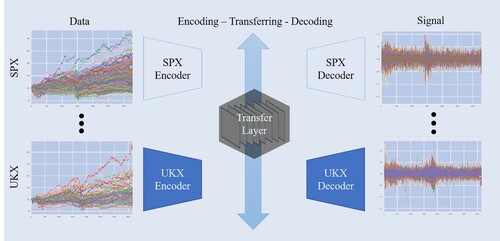
In this paper, we take a step towards overcoming these challenges and develop a full end-to-end learning system for global financial trading. We introduce QuantNet: an architecture that learns market-agnostic trends and uses them to learn superior market-specific trading strategies. Each market-specific model is composed of an encoder–decoder pair (figure 1). The encoder transforms market-specific data into an abstract latent representation that is processed by a global model shared by all markets, while the decoder learns a trading strategy based on the processed latent code returned by the global model. QuantNet leverages recent insights from transfer and meta-learning that suggest market-specific model components benefit from having separate parameters while being constrained by conditioning on an abstract global representation (Ruder et al. 2019). Furthermore, by incorporating multiple losses into a single network, our approach increases network regularization and avoids overfitting, as in Lee et al. (2015), Wang et al. (2015), Blumberg et al. (2019). We evaluate QuantNet on historical data across 3103 assets in 58 global equity markets. Against the best performing baseline Cross-sectional momentum (Jegadeesh and Titman 1993, Baz et al. 2015), QuantNet yields 51% higher Sharpe and 69% Calmar ratios. Also, we show the benefits of our approach, which yields improvements of 15% and 41% in Sharpe and Calmar ratios, respectively, over the comparable non-transfer learning variant.

Figure 1. QuantNet workflow: from market data to decoding/signal generation.

Our key contributions are: (i) a novel architecture for transfer learning across financial trading strategies; (ii) a novel learning objective to facilitate end-to-end training of trading strategies; and (iii) demonstrate that QuantNet can achieve significant improvements across global markets with an end-to-end learning system. To the best of our knowledge, this is the first paper that studies transfer learning as a means of improving end-to-end large scale learning of trading strategies.

2. Related work

Trading strategies with machine learning. Machine learning-based trading strategies have previously been explored in the setting of supervised learning (Aggarwal and Aggarwal 2017, Heaton et al. 2017, Fischer and Krauss 2018, Gu et al. 2020, Sezer et al. 2020) and reinforcement learning (Pendharkar and Cusatis 2018, Li et al. 2019, Gao et al. 2020, Zhang et al. 2020), nowadays with a major emphasis on deep learning methods. Broadly, these works differ from our proposed method as they do not use inter-market knowledge transfer and (in the case of methods based on supervised learning) tend to forecast returns/prices rather than to generate end-to-end trading signals. We provide an in-depth treatment in Section 3.1.

Deep learning. In the financial domain, data is predominantly sequential and, therefore, Recurrent Neural Network approaches like Long Short-term Memory (LSTM) networks are frequent. Heaton et al. (2017) demonstrates LSTMs networks as useful for asset returns movements and new ways to model volatility. It also has been used for trading (Lim et al. 2019), particularly coupling it with Reinforcement Learning methods (Zhang et al. 2020). Fischer and Krauss (2018) applied LSTMs to predict assets directional movement, benchmarking it against Random Forest and Logistic Regression. A popular application has been on NLP: Hiew et al. (2019) combined BERT (Devlin et al. 2018a) with LSTMs to build a Financial Sentiment Index; RNNs have also been used to read financial news articles (Vargas et al. 2017). LSTMs have also been used as the underlying model for model-based Reinforcement Learning (Lu 2017). Some other applications using Feed-forward nets, such as for hedging (Buehler et al. 2019) and to calibrate stochastic volatility models (Bayer et al. 2019), are other promising applications that can be potentially enhanced by the LSTM model. More generally, the reader interested in a literature review on financial time series forecasting with Deep Learning should refer to the work of Sezer et al. (2020).

Transfer learning. Transfer learning is a well-established method in machine learning (Caruana 1997, Pan and Yang 2009, Zhang 2019). It has been used in computer vision, medicine, and natural language processing (Blumberg et al. 2018, Kornblith et al. 2019, Radford et al. 2019). In financial systems, this paradigm has primarily been studied in the context of applying unstructured data, such as social media, to financial predictions (Araci 2019, Hiew et al. 2019). In a few occasions such methodologies have been applied to trading, usually combined with reinforcement learning and to a very limited pool of assets (Jeong and Kim 2019). We provide a thorough review of the area in Appendix 4.

The simplest and most common form of transfer learning pre-trains a model on a large dataset, hoping that the pre-trained model can be fine-tuned to a new task or domain at a later stage (Devlin et al. 2018a, Liu et al. 2019). While simple, this form of knowledge transfer assumes new tasks are similar to previous tasks, which can easily fail in financial trading where markets differ substantially. Our method instead relies on multi-task transfer learning (Caruana 1993, Baxter 1995, Caruana 1997, Ruder 2017). While this approach has previously been explored in a financial context (Ghosn and Bengio 1997, Bitvai and Cohn 2015), prior works either use full parameter sharing or share all but the final layer of relatively simple models. In contrast, we introduce a novel architecture that relies on encoding market-specific data into representations that pass through a global bottleneck for knowledge transfer. We provide a detailed discussion in Section 3.2.

3. QuantNet

We begin by reviewing end-to-end learning of financial trading in Section 3.1 and relevant forms of transfer learning in Section 3.2. We present our proposed architecture in Section 3.3.

3.1. Preliminaries: learning trading strategies

A financial market $M=(a^1,\dots ,a^n)$ consists of a set of n assets $a^j$; at each discrete time step t we have access to a vector of excess returns ${\mathit{r}}_t=(r_t^1,\dots ,r_t^n)\in {\mathbb{R}}^n$. The goal of a trading strategy f, parametrized by θ, is to map elements of a history $R_{m:t}=({\mathit{r}}_{t-m},\dots ,{\mathit{r}}_t)$ into a set of trading signals ${\mathit{s}}_t=(s_t^1,\dots ,s_t^n)\in {\mathbb{R}}^n$; ${\mathit{s}}_t=f_{\theta }\left(R_{m:t}\right)$. These signals constitute a market portfolio: a trader would buy one unit of an asset if $s_t^j=1$, sell one unit if $s_t^j=-1$, and close a position if $s_t^j=0$; any value in between $(-1,1)$ implies that the trader is holding/shorting a fraction of an asset. The goal is to produce a sequence of signals that maximize risk-adjusted returns. The most common approach is to model f as a moving average parametrized by weights $\theta =(W_1,\dots ,W_m)$, $W_i\in {\mathbb{R}}^{n\times n}$, where weights typically decreases exponentially or are hand-engineered and remain static (Avramovic et al. 2017, BarclayHedge 2017, Firoozye and Koshiyama 2019); (1) $\begin{array}{rl}{\mathit{s}}_t^{\mathrm{m}\mathrm{a}}& =\tau \left(f_{\theta }^{\mathrm{m}\mathrm{a}}\right(R_{t-m:t}\left)\right)\\ & =\tau \left(\sum _{k=t-m}^t{W}_k{\mathit{r}}_k\right),\tau :{\mathbb{R}}^n\to [-1,1{]}^n.\end{array}$(1) More advanced models rely on recurrence to form an abstract representation of the history up to time t; either by using Kalman filtering, Hidden Markov Models (HMM), or Recurrent Neural Networks (RNNs) (Fischer and Krauss 2018, Zhang et al. 2019). For our purposes, having an abstract representation of the history will be crucial to facilitate effective knowledge transfer, as it captures each market's dynamics, thereby allowing QuantNet to disentangle general and idiosyncratic patterns. We use the Long Short-Term Memory (LSTM) network (Hochreiter and Schmidhuber 1997, Gers et al. 1999), which is a special form of an RNN. LSTMs have been recently explored to form the core of trading strategy systems (Fischer and Krauss 2018, Hiew et al. 2019, Sezer et al. 2020). For simplicity, we present the RNN here and refer the interested reader to (Hochreiter and Schmidhuber 1997, Gers et al. 1999) or Appendix 3. The RNN is defined by introducing a recurrent operation that updates a hidden representation $\mathit{h}$ recurrently conditional on the input $\mathit{r}$: (2) $\begin{array}{rl}{\mathit{s}}_t^{\mathrm{R}\mathrm{N}\mathrm{N}}& =\tau (W_s{\mathit{h}}_t+{\mathit{b}}_s),\\ {\mathit{h}}_t& =f_{\theta }^{\mathrm{R}\mathrm{N}\mathrm{N}}({\mathit{r}}_{t-1},{\mathit{h}}_{t-1})=\sigma (W_r{\mathit{r}}_{t-1}+W_h{\mathit{h}}_{t-1}+\mathit{b}),\end{array}$(2) where σ is an element-wise activation function and $\theta =(W_r,W_h,\mathit{b})$ parameterize the RNN. The LSTM is similarly defined but adds a set of gating mechanisms to enhance the memory capacity and gradient flow through the model. To learn the parameters of the RNN, we use truncated backpropagation through time (TBPTT; Sutskever 2013), which backpropagates a loss $\mathcal{L}$ through time to the parameters of the RNN, truncating after K time steps.

3.2. Preliminaries: transfer learning

Transfer learning (Caruana 1997, Pan and Yang 2009, Ruder 2017, Zhang 2019) embodies a set of techniques for sharing information obtained on one task, or market, when learning another task (market). In the simplest case of pre-training (Devlin et al. 2018a, Liu et al. 2019), for example, we would train a model in a market $M_2$ by initializing its parameters to the final parameters obtained in market $M_1$. While such pre-training can be useful, there is no guarantee that the parameters obtain on task $M_1$ will be useful for learning task $M_2$.

In multi-task transfer-learning, we have a set of $\mathcal{M}=(M_1,\dots ,M_N)$ markets that we aim to learn simultaneously. The multi-task literature often presumes one $M_i$ is the main task, and all others are auxiliary—their sole purpose is to improve final performance on $M_i$ (Caruana 1997, Gibiansky et al. 2017). A common problem in multi-task transfer is therefore how to assign weights $w_i$ to each market-specific loss ${\mathcal{L}}^i$ when setting the multi-task objective $\mathcal{L}=\sum _i{w}_i{\mathcal{L}}^i$. This is often a hyper-parameter that needs to be tuned (Ruder 2017).

As mentioned above, this poses a challenge in our case as markets are typically not homogeneous. Instead, we turn to sequential multi-task transfer learning (Ruder et al. 2019), which learns one model $f^i$ per market $M_i$, but partition the parameters of the model into a set of market-specific parameters ${\theta }^i$ and a set of market-agnostic parameters ϕ. In doing so, market-specific parameters are free to specialize on the problem at hand, while market-agnostic parameters capture signals from all markets. However, in contrast to standard approaches to multi-task transfer learning, which either share all parameters, a set from the final layer(s) or share no parameters, we take inspiration from recent advances in meta-learning (Lee and Choi 2018, Zintgraf et al. 2018, Flennerhag et al. 2020a), which shows that more flexible parameter-sharing schemes can reap a greater reward. In particular, interleaving shared and market-specific parameters can be seen as learning both shared representation and a shared optimizer (Flennerhag et al. 2020a).

We depart from previous work by introducing an encoder–decoder setup (Cho et al. 2014b) within financial markets. Encoders learn to represent market-specific information, such as internal fiscal and monetary conditions, development stage, and so on, while a global shared model learns to represent market-agnostic dynamics such as global economic outlook, contagion effects (via financial crises). The decoder uses these sources of information to produce a market-specific trading strategy. With these preliminaries, we now turn to QuantNet, our proposed method for end-to-end multi-market financial trading.

3.3. QuantNet

Architecture. Figure 1 portrays the QuantNet architecture. In QuantNet, we associate each market $M_i$ with an encoder–decoder pair, where the encoder ${\mathrm{enc}}^i$ and the decoder ${\mathrm{dec}}^i$ are both LSTMs networks. Both models maintain a separate hidden state, ${\mathit{e}}^i$ and ${\mathit{d}}^i$, respectively. When given a market return vector ${\mathit{r}}^i$, the encoder produces an encoding ${\mathit{e}}^i$ that is passed onto a market-agnostic model ω, which modifies the market encoding into a representation ${\mathit{z}}^i$: (3) ${\mathit{z}}_t^i=\omega \left({\mathit{e}}_t^i\right),\mathrm{w}\mathrm{h}\mathrm{e}\mathrm{r}\mathrm{e}{\mathit{e}}_t^i={\mathrm{enc}}^i({\mathit{r}}_{t-1}^i,{\mathit{e}}_{t-1}^i).$(3) Because ω is shared across markets, ${\mathit{z}}^i$ reflects market information from market $M^i$ 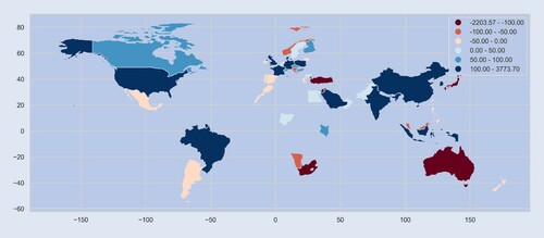while taking global information (as represented by ω) into account. This bottleneck enforces local representations that are aware of global dynamics, and so we would expect similar markets to exhibit similar representations (Mikolov et al. 2013). We demonstrate this empirically in figure 2, which shows how each market is being represented internally by QuantNet. We apply hierarchical clustering on hidden representation from the encoder (see also dendrogram in appendix 7) using six centroids. We observe clear geo-economical structure emerging from QuantNet—without it receiving any such geographical information. $C5$ consists mainly of small European equity markets (Spain, Netherlands, Belgium, and France)—all neighbours; $C6$ encompass developed markets in Europe and Americas, such as the UK, Germany, the USA, and their respective neighbours Austria, Poland, Switzerland, Sweden, Denmark, Canada, and Mexico. Other clusters are more refined: $C2$ for instance contains most developed markets in Asia like Japan, Hong Kong, Korea, and Singapore, while $C3$ represents Asia and Pacific emerging markets: China, India, and some respective neighbours (Pakistan, Philippines, Taiwan).

Figure 2. World map depicting the different clusters formed from the scores of QuantNet encoder. For visualization purposes, we have picked the market with the biggest market capitalization to represent the country in the cluster.

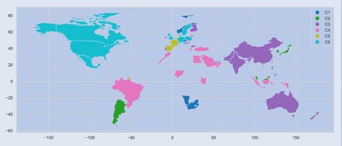
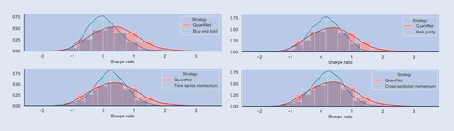
Figure 3. Histogram of Sharpe ratio contrasting QuantNet with baseline strategies.

We experiment with different functional forms for ω; adding complexity to ω can allow more sophisticated representations, but simpler architectures enforce an information bottleneck (Yu and Principe 2019). Indeed we find experimentally that a simple linear layer works better than an LSTM (see Appendix 8), which is in line with general wisdom on encoder–decoder architectures (Cho et al. 2014a, 2014b).

Given a representation ${\mathit{z}}_t^i$, we produce a market-specific trading strategy by decoding this abstract representation into a hidden market-specific state ${\mathit{d}}_t^i$; this state represents the trading history in market $M^i$, along with the history of global dynamics, and is used learn a market-specific strategy (4) ${\mathit{s}}_t^i=f^i\left({\mathit{d}}_t^i\right)=\tanh (W^i{\mathit{d}}_t^i+{\mathit{b}}^i),\mathrm{w}\mathrm{h}\mathrm{e}\mathrm{r}\mathrm{e}{\mathit{d}}_t^i={\mathrm{dec}}^i({\mathit{z}}_t^i,{\mathit{d}}_{t-1}^i).$(4) While $f^i$ can be any model, we found a simple linear layer sufficient due to the expressive capacity of the encoder–decoder pair. For a non-leveraged trading strategy, we chose tanh as our activation function, which bounds the trading signal ${\mathit{s}}_t^i\in (-1,1{)}^n$ (Acar and Satchell 2002, Voit 2013).

From equation (4(4) ${\mathit{s}}_t^i=f^i\left({\mathit{d}}_t^i\right)=\tanh (W^i{\mathit{d}}_t^i+{\mathit{b}}^i),\mathrm{w}\mathrm{h}\mathrm{e}\mathrm{r}\mathrm{e}{\mathit{d}}_t^i={\mathrm{dec}}^i({\mathit{z}}_t^i,{\mathit{d}}_{t-1}^i).$(4) ), we can see how transfer learning affects both trading and learning. During trading, by processing a market encoding ${\mathit{e}}_t^i$ through a shared global layer ω, we impose a bottleneck such that any trading strategy is forced to act on the globally conditioned information in ${\mathit{z}}_t^i$. During learning, market-specific trading is unrestricted in its parameter updates, but gradients are implicitly modulated through the conditioned input; particularly for the encoder, which must service its corresponding decoder by passing through the global layer ω. Concretely, given a market loss function ${\mathcal{L}}^i$ with error signal ${\delta }^i=d\mathcal{L}/d{\mathit{s}}^i$, market-specific gradients are given by (5) $\begin{array}{rl}{\mathrm{\nabla }}_{{\theta }_{{\mathrm{d}\mathrm{e}\mathrm{c}}^i}^i}{\mathcal{L}}^i\left({\mathit{s}}_t^i\right)& ={\delta }_t^i\frac{\mathrm{\partial }{\mathit{s}}_t^i}{\mathrm{\partial }{\mathit{d}}_t^i}\frac{\mathrm{\partial }{\mathrm{dec}}^i}{\mathrm{\partial }{\theta }_{{\mathrm{d}\mathrm{e}\mathrm{c}}^i}^i}({\mathit{z}}_t^i;{\mathit{d}}_{t-1}^i),\\ {\mathrm{\nabla }}_{{\theta }_{{\mathrm{e}\mathrm{n}\mathrm{c}}^i}^i}{\mathcal{L}}^i\left({\mathit{s}}_t^i\right)& ={\delta }_t^i\frac{\mathrm{\partial }{\mathit{s}}_t^i}{\mathrm{\partial }{\mathit{d}}_t^i}\frac{\mathrm{\partial }{\mathit{d}}_t^i}{\mathrm{\partial }{\mathit{z}}_t^i}\frac{\mathrm{\partial }{\mathit{z}}_t^i}{\mathrm{\partial }{\mathit{e}}_t^i}\frac{\mathrm{\partial }{\mathrm{enc}}^i}{\mathrm{\partial }{\theta }_{{\mathrm{e}\mathrm{n}\mathrm{c}}^i}^i}({\mathit{r}}_t^i;{\mathit{e}}_{t-1}^i).\end{array}$(5) The gradient of the decoder is largely free but must adapt to the representation produced by the encoder and the global model. These, in turn, are therefore influenced by what representations are useful for the decoder. In particular, the gradient of the encoder must pass through the global model, which acts as a preconditioner of the encoder parameter gradient, thereby encoding an optimizer (Flennerhag et al. 2020b). Finally, to see how global information gets encoded in the global model, under a multi-task loss, its gradients effectively integrate out idiosyncratic market correlations: (6) ${\mathrm{\nabla }}_{\varphi }\mathcal{L}({\mathit{s}}_t^1,\dots ,{\mathit{s}}_t^n)=\sum _{i=1}^n{\delta }_t^i\frac{\mathrm{\partial }{\mathit{s}}_t^i}{\mathrm{\partial }{\mathit{d}}_t^i}\frac{\mathrm{\partial }{\mathit{d}}_t^i}{\mathrm{\partial }{\mathit{z}}_t^i}\frac{\mathrm{\partial }\omega }{\mathrm{\partial }\varphi }\left({\mathit{e}}_t^i\right).$(6)

Learning objective. To effectively learn trading strategies with QuantNet, we develop a novel learning objective based on the Sharpe ratio (Sharpe 1994, Bailey and Lopez de Prado 2012, Harvey and Liu 2015). Prior work on financial forecast tends to rely on Mean Squared Error (MSE) (Heaton et al. 2017, Hiew et al. 2019, Gu et al. 2020), as does most work on learning trading strategies. A few works have instead considered other measurements (Fischer and Krauss 2018, Zhang et al. 2019, 2020). In particular, there are strong theoretical and empirical reasons for considering the Sharpe ratio instead of MSE—in fact, MSE minimization is a necessary, but not sufficient condition to maximize the profitability of a trading strategy (Bengio 1997, Acar and Satchell 2002, Koshiyama and Firoozye 2019b). Since some assets are more volatile than others, the Sharpe ratio helps to discount the optimistic average returns by taking into account the risk faced when traded those assets. Also, it is widely adopted by quantitative investment strategists to rank different strategies and funds (Sharpe 1994, Bailey and Lopez de Prado 2012, Harvey and Liu 2015).

To compute each market Sharpe ratio at a time t, truncated to backpropagation through time for k steps (to t−k), considering excess daily returns, we first compute the per-asset Sharpe ratio (7) ${\rho }_{t,j}^i=\left({\mu }_{t-k:t,j}^i\right)/\left({\sigma }_{t-k:t,j}^i\right)\cdot \sqrt{252},$(7) where ${\mu }_{t,j}^i$ is the average return of the strategy for asset j and ${\sigma }_t^j$ is its respective the standard deviation. The $\sqrt{252}$ factor is included in computing the annualized Sharpe ratio. The market loss function and the QuantNet objective are given by averaging over assets and markets, respectively: (8) $\begin{array}{rl}\mathcal{L}\left({\{{\mathit{s}}_{t-k:t}^i,{\mathit{r}}_{t-k:t}^i\}}_{i=1}^N\right)& =\frac{1}{N}\sum _{i=1}^N{\mathcal{L}}^i({\mathit{s}}_{t-k:t}^i,{\mathit{r}}_{t-k:t}^i),\\ {\mathcal{L}}^i({\mathit{s}}_{t-k:t}^i,{\mathit{r}}_{t-k:t}^i)& =\frac{1}{n}\sum _{j=1}^n{\rho }_{t,j}^i.\end{array}$(8)

Training. To train QuantNet, we use stochastic gradient descent. To obtain a gradient update, we first sample mini-batches of m markets from the full set $\mathcal{M}=(M_1,\dots ,M_N)$ to obtain an empirical expectation over markets. Given these, we randomly sample a time step t and run the model from t−k to t, from which we obtain market Sharpe ratios. Then, we compute QuantNet loss function and differentiate through time into all parameters. We pass this gradient to an optimizer, such as Adam, to take one step on the model's parameters. This process is repeated until the model converges.

4. Results

This section assesses QuantNet performance compared to baselines and a No Transfer strategy defined by a single LSTM of the same dimensionality as the decoder architecture (number of assets), as defined in equation (2(2) $\begin{array}{rl}{\mathit{s}}_t^{\mathrm{R}\mathrm{N}\mathrm{N}}& =\tau (W_s{\mathit{h}}_t+{\mathit{b}}_s),\\ {\mathit{h}}_t& =f_{\theta }^{\mathrm{R}\mathrm{N}\mathrm{N}}({\mathit{r}}_{t-1},{\mathit{h}}_{t-1})=\sigma (W_r{\mathit{r}}_{t-1}+W_h{\mathit{h}}_{t-1}+\mathit{b}),\end{array}$(2) ). Next section presents the main experimental setting, with the subsequent ones providing: (i) a complete comparison of QuantNet with other trading strategies; (ii) an in-depth comparison of QuantNet versus the best No Transfer strategy; and (iii) analysis on market conditions that facilitate transfer under QuantNet. We provide an ablation study and sensitivity analysis of QuantNet in appendix 8.

4.1. Experimental setting

Datasets. Appendix 1 provides a full table listing all 58 markets used. We tried to find a compromise between the number of assets and sample size, hence for most markets, we were unable to use the full list of constituents. We aimed to collect daily price data ranging from 03/01/2000 to 15/03/2019, but for most markets it starts roughly around 2010. Finally, due to restrictions from our Bloomberg license, we were unable to access data for some important equity markets, such as Italy and Russia.

Evaluation. We compared QuantNet with four other traditional and widely adopted and researched trading strategies. Below we briefly expose each one of them as well as provide some key references:

• Buy and hold: This strategy is simply purchase a unit of stock and hold it, that is, ${\mathit{s}}_t^{\mathrm{B}\mathrm{a}\mathrm{H}}:=\mathbf{1}$ for all assets in a market. Active trading strategies are supposed to beat this passive strategy, but in some periods just holding an S&P 500 portfolio passively outperforms many active managed funds (Elton et al. 2019, Dichtl 2020).

• Risk parity: This approach trade assets in a certain market such that they contribute as equally as possible to the portfolio overall volatility. A simple approach used is to compute signals per asset as (9) $s_{t,j}^{\mathrm{R}\mathrm{P}}:=\frac{\frac{1}{{\sigma }_{t:t-252}^j}}{\frac{1}{\sum _{j=1}^n{\sigma }_{t:t-252}^j}}$(9) with ${\sigma }_{t:t-252}^j$ as the rolling 252 days (≈1 year) volatility of asset j. Interest in the risk parity approach has increased since the late 2000s financial crisis as the risk parity approach fared better than traditionally constructed portfolios (Choueifaty and Coignard 2008, Martellini 2008, Du Plessis and Hallerbach 2016).

• Time series momentum: This strategy, also called trend momentum or trend-following, suggests going long in assets which have had recent positive returns and short assets which have had recent negative returns. It is possibly one of the most adopted and researched strategy in finance (Moskowitz et al. 2012, Daniel and Moskowitz 2016, Baltzer et al. 2019). For a given asset, the signal is computed as (10) $s_{t,j}^{\mathrm{T}\mathrm{S}\mathrm{M}\mathrm{O}\mathrm{M}}:={\mu }_{t:t-252}^j$(10) with 252 days (≈ 12 months, ≈ 1 year) the typical lookback period to compute the average return ${\mu }_{t:t-252}^j$ of asset j.

• Cross-sectional momentum: The cross-sectional momentum strategy as defined by is a long-short zero-cost portfolio that consists of securities with the best and worst relative performance over a lookback period (Jegadeesh and Titman 1993, Baz et al. 2015, Feng et al. 2020). It works similarly as time series momentum, with the addition of screening weakly performing and underperforming assets. For a given market, the signal can be computed as (11) $s_{t,j}^{\mathrm{C}\mathrm{S}\mathrm{M}\mathrm{O}\mathrm{M}}:=\{\begin{array}{ll}{\mu }_{t:t-252}^j,& \mathrm{i}\mathrm{f}{\mu }_{t:t-252}^j>Q_{1-q}\\ & ({\mu }_{t:t-252}^1,\dots ,{\mu }_{t:t-252}^n)\\ -{\mu }_{t:t-252}^j,& \mathrm{i}\mathrm{f}{\mu }_{t:t-252}^j<Q_q\\ & ({\mu }_{t:t-252}^1,\dots ,{\mu }_{t:t-252}^n)\\ 0,& \mathrm{o}\mathrm{t}\mathrm{h}\mathrm{e}\mathrm{r}\mathrm{w}\mathrm{i}\mathrm{s}\mathrm{e}\end{array}$(11) with $Q_q({\mu }_{t:t-252}^1,\dots ,{\mu }_{t:t-252}^n)$ representing the qth quantile of the assets average returns. A signal for going long (short) is produced if the asset j is at the top (bottom) quantile of the distribution. In our experiments, we used the typical value of q = 0.33.

Since running an exhaustive search is computationally prohibitive, we opted to use random search as our hyperparameter optimization method (Bergstra and Bengio 2012). Appendix B provides full description of the hyperparameter search protocol. We sampled a total of 200 values in between those ranges. We report results for trained models under best hyperparameters on validation sets; for each dataset we construct a training and validation set, where the latter consists of the last 752 observations of each time series (around 3 years). We have used 3 Month London Interbank Offered Rate in US Dollar as the reference rate to compute excess returns. We have also reported Calmar ratios, Annualized Returns and Volatility, Downside risk, Sortino ratios, Skewness and Maximum drawdowns (Young 1991, Sharpe 1994, Eling and Schuhmacher 2007, Rollinger and Hoffman 2013). All metrics were computed using the Python package empyrical (https://github.com/quantopian/empyrical).

4.2. Empirical evaluation

Baseline comparison. Table 1 presents median and mean absolute deviation (in brackets) performance of the different trading strategies on 3103 stocks across all markets analysed. The best baseline is Cross-sectional Momentum (CS Mom), yielding an SR of 0.23 and CR of 0.14. QuantNet outperforms CS Mom, yielding 51% higher SR and 69% higher CR. No Transfer LSTM and Linear outperform this baseline as well, but not to the same extent as QuantNet.

Table 1. Median and mean absolute deviation (in brackets) performance on 3103 stocks across all markets analysed.

Metric	Buy and hold	Risk parity	TS Mom	CS Mom	No Transfer LSTM	No Transfer Linear	QuantNet
Ann Ret	0.000020	0.000193	0.000050	0.000042	0.002508	0.001537	0.005377
	(0.13433)	(0.00270)	(0.00019)	(0.00019)	(0.07645)	(0.08634)	(0.02898)
Ann Vol	0.287515	0.001536	0.000290	0.000270	0.008552	0.007768	0.023665
	(0.10145)	(0.00537)	(0.00036)	(0.00036)	(0.13455)	(0.14108)	(0.04540)
CR	0.000040	0.095516	0.139599	0.143195	0.158987	0.169345	0.241255
	(0.33583)	(0.29444)	(1.05288)	(1.18751)	(0.55762)	(0.57170)	(0.59968)
DownRisk	0.202361	0.001076	0.000195	0.000178	0.005656	0.005124	0.015734
	(0.07042)	(0.00361)	(0.00024)	(0.00025)	(0.09223)	(0.09553)	(0.03291)
Kurt	5.918386	6.165916	13.333863	18.112853	16.87256	15.73864	16.19961
	(10.2515)	(13.9426)	(19.2278)	(24.4672)	(30.2204)	(31.0395)	(24.7336)
MDD	−0.419984	−0.002935	−0.000488	−0.000444	−0.014564	−0.01286	−0.03847
	(0.14876)	(0.00987)	(0.00082)	(0.00081)	(0.16724)	(0.17820)	(0.07881)
SR	0.000051	0.155560	0.226471	0.234583	0.304244	0.306572	0.354776
	(0.42324)	(0.42028)	(0.40627)	(0.41547)	(0.51552)	(0.51182)	(0.57218)
Skew	−0.087282	−0.092218	0.427237	0.568364	0.256736	0.171629	0.297182
	(0.82186)	(0.96504)	(1.28365)	(1.60612)	(1.77245)	(1.74804)	(1.66854)
SortR	0.217621	0.220335	0.333685	0.349124	0.443422	0.454035	0.52196
	(0.59710)	(0.61883)	(1.02616)	(0.633953)	(0.78525)	(0.86715)	(1.02465)

TS Mom, time series momentum and CS Mom, cross-section momentum. We highlighted in bold only the metrics where a comparison can be made, like Sharpe ratios, Calmar ratios, Kurtosis, Skewness, and Sortino ratios.

QuantNet vs no transfer linear. When comparing QuantNet and No Transfer Linear strategies performance ( table 1), we observe an improvement of about 15% on SR and 41% on CR. This improvement increases the number of assets yielding SRs above 1.0 from 432 to 583, smaller Downside Risk (DownRisk), higher Skew and Sortino ratios (SortR). Statistically, QuantNet significantly outperform No Transfer both in Sharpe ($W=\mathrm{2,215,630}$, p-value < 0.01) and Calmar ($W=\mathrm{2,141,782}$, p-value < 0.01) ratios. This discrepancy manifests in statistical terms, with the Kolmogorov–Smirnov statistic indicating that these distributions are meaningfully different (KS = 0.053, p-value < 0.01).

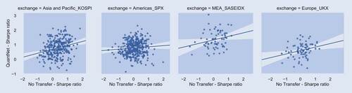
Figure 4 outlines the average SR across the 58 markets, ordered by No Transfer strategy performance. In SR terms, QuantNet outperforms No Transfer in its top 5 markets and dominates the bottom 10 markets where No Transfer yields negative results, both in terms of SR and CR ratios. Finally, in 7 of the top 10 largest ones (RTY, SPX, KOSPI, etc.), QuantNet also outperforms No Transfer. Figure 5(a) presents cumulative returns charts in a set of large regional markets, such as United States S&P 500 components (SPX Index), United Kingdom FTSE 100 (UKX Index), Korea Composite Index (KOSPI Index), and Saudi Arabia Tadawul All Shares (SASEIDX Index). Across regions, we observe 2–10 times order of magnitude improvement in SRs and CRs by QuantNet, with similar benefits in Sortino ratios, Downside risks, and Skewness. Appendix 5 provides further analysis.

Figure 4. Average Sharpe ratios of QuantNet and No Transfer across 58 equity markets.

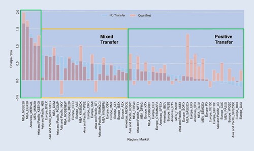
Figure 5. (a) Average cumulative returns (%) of SPX Index, UKX Index, KOSPI Index and SASEIDX Index contrasting QuantNet and No Transfer. Average Sharpe ratio difference between QuantNet versus No Transfer, aggregated by sample size (b) and number of assets per market (c)—in both we have subtracted QuantNet SR from No Transfer SR to reduce cross-asset variance and baseline effect.

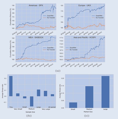
QuantNet features. One of the key features of transfer learning is its ability to provide meaningful solutions in resource-constrained scenarios—sample size, features, training budget, etc. With QuantNet this pattern persists; figure 5(b) presents the average SR grouped based on market sample size in the training set. As transfer-learning would predict, we observe large gains to transfer in markets with tiny sample size (1444–1823 samples or ≈6–7 years) where fitting a model on only local market data yields poor performance. Further, gains from transfer generally decay as sample sizes increase. Interestingly, we find that medium-sized markets (2200–2576 samples or ≈10 years of data) do not benefit from transfer, suggesting that there is room for improvement in the design of our transfer bottleneck ω, an exciting avenue for future research. Another vital feature is coping with market size—figure 5(c) outlines QuantNet performance in terms of average SR. It demonstrates that the bigger the market, the better QuantNet will perform.

5. Conclusion

In this paper, we introduce QuantNet: an architecture that learns market-agnostic trends and use these to learn superior market-specific trading strategies. QuantNet uses recent advances in transfer- and meta-learning, where market-specific parameters are free to specialize on the problem at hand, while market-agnostic parameters capture signals from all markets. QuantNet takes a step towards end-to-end global financial trading that can deliver superior market returns. In a few big regional markets, such as S&P 500, FTSE 100, KOSPI and Saudi Arabia Tadawul All Shares, QuantNet showed 2–10 times improvement in SR and CR. QuantNet also generated positive and statistically significant alpha according to Fama-French 5 factors model ( appendix 6). An avenue of future research is to identify the functional form of a global transfer layer that can deliver strong performance also on markets where mixed transfer occurred, such as those with medium sample size. Furthermore, by analysing QuantNet encoders, it appears that they are mapping and structuring the markets according to their development stage and geographical proximity.

In future works, we aim to investigate different architectures, such as Transformer layers, as it seems that they are providing significant outperformance in other tasks with sequence data (mainly text). Expanding the empirical evaluation to include other asset classes beyond equities, such as foreign exchange, interest rate swaps, or commodities can potentially improve the overall results since it can provide additional knowledge to trade some equities and vice versa.

Disclosure statement

No potential conflict of interest was reported by the author(s).

Additional information

Funding

This work was supported by CNPQ [grant number 0001].

Notes

1 A more generic definition, that works for unsupervised and reinforcement learning, demands that along with every task ${\mathcal{T}}_i$ we have an objective function $f_i$.

2 We should note that there are other possibilities, but they fall into Unsupervised or Reinforcement transfer learning. These other paradigms fall outside the scope of this work, which is mostly interested in (Semi-) Supervised transfer learning.

Appendix 1.

Datasets

Table A1 presents the datasets/markets used to empirically evaluate QuantNet. All the data was obtained via Bloomberg, with the description of each market/index and its constituents at https://www.bloomberg.com; for instance, SPX can be found by searching using the following link: https://www.bloomberg.com/quote/SPX:IND. We tried to find a compromise between number of assets and sample size, hence for most markets we were unable to use the full list of constituents. We aimed to collect daily price data ranging from 03/01/2000 to 15/03/2019, but for most markets it starts roughly around 2010. Finally, due to restrictions from our Bloomberg license, we were unable to access data for some important equity markets, such as Italy and Russia. Full list with assets and respective exchange can be found at: https://www.dropbox.com/s/eobhg2w8ithbgsp/AssetsExchangeList.xlsx?dl=0

Table A1. Markets used during our experiment.

Region	Index/Market	Country	# Samples	# Assets	Region	Index/Market	Country	# Samples	# Assets
Americas	IBOV	Brazil	3250	29	Europe	HEX	Finland	1882	65
Americas	MERVAL	Argentina	3055	11	Europe	IBEX	Spain	3499	23
Americas	MEXBOL	Mexico	3002	19	Europe	ISEQ	Ireland	2888	14
Americas	RTY	US	2356	554	Europe	KFX	Denmark	3345	15
Americas	SPTSX	Canada	3173	129	Europe	OBX	Norway	2812	17
Americas	SPX	US	3291	376	Europe	OMX	Sweden	3453	29
Asia and Pacific	AS51	Australia	2363	91	Europe	PX	Czechia	3374	5
Asia and Pacific	FBMKLCI	Malaysia	3131	23	Europe	SBITOP	Slovenia	2995	6
Asia and Pacific	HSI	China	2599	37	Europe	SMI	Switzerland	3948	19
Asia and Pacific	JCI	Indonesia	2007	44	Europe	SOFIX	Bulgaria	1833	5
Asia and Pacific	KOSPI	South Korea	3041	297	Europe	UKX	UK	3664	75
Asia and Pacific	KSE100	Pakistan	2036	41	Europe	VILSE	Lithuania	2765	5
Asia and Pacific	NIFTY	India	3066	38	Europe	WIG20	Poland	3449	8
Asia and Pacific	NKY	Japan	3504	186	Europe	XU100	Turkey	2545	76
Asia and Pacific	NZSE50FG	New Zealand	3258	21	MEA	DFMGI	UAE	2184	11
Asia and Pacific	PCOMP	Philippines	3013	16	MEA	DSM	Qatar	2326	16
Asia and Pacific	SHSZ300	China	2881	18	MEA	EGX30	Egypt	1790	22
Asia and Pacific	STI	Singapore	2707	27	MEA	FTN098	Namibia	1727	16
Asia and Pacific	TWSE	Taiwan	3910	227	MEA	JOSMGNFF	Jordan	2287	15
Europe	AEX	Netherlands	4083	17	MEA	KNSMIDX	Kenya	1969	14
Europe	ASE	Greece	2944	51	MEA	KWSEPM	Kuwait	2785	11
Europe	ATX	Austria	3511	13	MEA	MOSENEW	Morocco	2068	27
Europe	BEL20	Belgium	3870	14	MEA	MSM30	Oman	2069	24
Europe	BUX	Hungary	3753	8	MEA	NGSE30	Nigeria	1761	25
Europe	BVLX	Portugal	3269	17	MEA	PASISI	Palestine	1447	5
Europe	CAC	France	3591	36	MEA	SASEIDX	Saudi Arabia	1742	71
Europe	CRO	Croatia	1975	13	MEA	SEMDEX	Mauritius	2430	5
Europe	CYSMMAPA	Cyprus	2056	42	MEA	TA-35	Israel	2677	23
Europe	DAX	Germany	3616	27	MEA	TOP40	South Africa	2848	34

MEA, Middle East and Africa.

Appendix 2.

Evaluation

Baselines. We compared QuantNet with four other traditional and widely adopted and researched trading strategies. Below we briefly expose each one of them as well as provide some key references:

• Buy and hold: This strategy is simply purchase a unit of stock and hold it, that is, ${\mathit{s}}_t^{\mathrm{B}\mathrm{a}\mathrm{H}}:=\mathbf{1}$ for all assets in a market. Active trading strategies are supposed to beat this passive strategy, but in some periods just holding an S&P 500 portfolio passively outperforms many active managed funds (Elton et al. 2019, Dichtl 2020).

• Risk parity: This approach trade assets in a certain market such that they contribute as equally as possible to the portfolio overall volatility. A simple approach used is to compute signals per asset as (A1) $s_{t,j}^{\mathrm{R}\mathrm{P}}:=\frac{\frac{1}{{\sigma }_{t:t-252}^j}}{\frac{1}{\sum _{j=1}^n{\sigma }_{t:t-252}^j}}$(A1) with ${\sigma }_{t:t-252}^j$ as the rolling 252 days (≈1 year) volatility of asset j. Interest in the risk parity approach has increased since the late 2000s financial crisis as the risk parity approach fared better than traditionally constructed portfolios (Choueifaty and Coignard 2008, Martellini 2008, Du Plessis and Hallerbach 2016).

• Time series momentum: This strategy, also called trend momentum or trend-following, suggests going long in assets which have had recent positive returns and short assets which have had recent negative returns. It is possibly one of the most adopted and researched strategy in finance (Moskowitz et al. 2012, Daniel and Moskowitz 2016, Baltzer et al. 2019). For a given asset, the signal is computed as (A2) $s_{t,j}^{\mathrm{T}\mathrm{S}\mathrm{M}\mathrm{O}\mathrm{M}}:={\mu }_{t:t-252}^j$(A2) with 252 days (≈12 months, ≈1 year) the typical lookback period to compute the average return ${\mu }_{t:t-252}^j$ of asset j.

• Cross-sectional momentum: The cross-sectional momentum strategy as defined by is a long-short zero-cost portfolio that consists of securities with the best and worst relative performance over a lookback period (Jegadeesh and Titman 1993, Baz et al. 2015, Feng et al. 2020). It works similarly as time series momentum, with the addition of screening weakly performing and underperfoming assets. For a given market, the signal can be computed as (A3) $s_{t,j}^{\mathrm{C}\mathrm{S}\mathrm{M}\mathrm{O}\mathrm{M}}:=\{\begin{array}{ll}{\mu }_{t:t-252}^j,& \mathrm{i}\mathrm{f}{\mu }_{t:t-252}^j>Q_{1-q}\\ & ({\mu }_{t:t-252}^1,\dots ,{\mu }_{t:t-252}^n)\\ -{\mu }_{t:t-252}^j,& \mathrm{i}\mathrm{f}{\mu }_{t:t-252}^j<Q_q\\ & ({\mu }_{t:t-252}^1,\dots ,{\mu }_{t:t-252}^n)\\ 0,& \mathrm{o}\mathrm{t}\mathrm{h}\mathrm{e}\mathrm{r}\mathrm{w}\mathrm{i}\mathrm{s}\mathrm{e}\end{array}$(A3) with $Q_q({\mu }_{t:t-252}^1,\dots ,{\mu }_{t:t-252}^n)$ representing the qth quantile of the assets average returns. A signal for going long (short) is produced if the asset j is at the top (bottom) quantile of the distribution. In our experiments, we used the typical value of q = 0.33.

Hyperparameters. Table A2 outlines the settings for QuantNet and No Transfer strategies. Since running an exhaustive search is computationally prohibitive, we opted to use random search as our hyperparameter optimization strategy (Bergstra and Bengio 2012). We randomly sampled a total of 200 values in between those ranges, giving larger bounds for configurations with less hyperparameters (No Transfer linear and QuantNet Linear-Linear). After selecting the best hyperparameters, we applied them in a holdout-set consisting of the last 752 observations of each time series (around 3 years). The metrics and statistics in this set are reported in our results section. After a few warm-up runs, we opted to use 2000 training steps as a good balance between computational time and convergence. We trained the different models using the stochastic gradient descent optimizer AMSgrad (Reddi et al. 2019), a variant of the now ubiquitously used Adam algorithm.

Table B1. No Transfer and QuantNet hyperparameters and configurations investigated.

	No transfer		QuantNet (encoder/decoder-transfer layer)
Hyper-parameter	Linear	LSTM	Linear-linear	Linear-LSTM	LSTM-linear	LSTM-LSTM
Batch size (L)	16-128	16-128	16-128	16-96	16-96	16-96
Sequence length (p)	21-504	21-504	21-504	21-252	21-252	21-252
Learning rate	0.0001-0.1	0.0001-0.1	0.0001-0.1	0.0001-0.5	0.0001-0.5	0.0001-0.5
E/D # layers		1-2			1-2	1-2
E/D dropout		0.1-0.9			0.1-0.9	0.1-0.9
TL # layers				1-2		1-2
TL dropout				0.1-0.9		0.1-0.9
TL dimension (N)	10, 25, 50, 100
Training steps	2000

Financial metrics. We have used 3 Month London Interbank Offered Rate in US Dollar as the reference rate to compute excess returns. Most of the results focus on Sharpe ratios, but in many occasions we have also reported Calmar ratios, Annualized Returns and Volatility, Downside risk, Sortino ratios, Skewness and Maximum drawdowns (Young 1991, Sharpe 1994, Eling and Schuhmacher 2007, Rollinger and Hoffman 2013).

Appendix 3.

LSTMs and QuantNet's architecture

Given as inputs a sequence of returns from a history $R_{m:t}=({\mathit{r}}_{t-m}^i,\dots ,{\mathit{r}}_t^i)$ of market i, below we outline QuantNet's input to trading signal (output) mapping, considering the LSTM and Linear models (Hochreiter and Schmidhuber 1997, Gers et al. 1999, Flennerhag et al. 2018) defined by the gating mechanisms: (A4) $\begin{array}{rl}& {\mathit{e}}_t^i=\mathrm{L}\mathrm{S}\mathrm{T}\mathrm{M}({\mathit{r}}_{t-1}^i,{\mathit{e}}_{t-1}^i)\\ & =\{\begin{array}{l}{\mathit{u}}_t^{s\in \{p,f,o,g\}}=W_{{\mathit{e}}^i}^{\left(s\right)}{\mathit{r}}_{t-1}+V_{{\mathit{e}}^i}^{\left(s\right)}{\mathit{e}}_{t-1}^i+{\mathit{b}}_{{\mathit{e}}^i}^{\left(s\right)}\\ {\mathit{c}}_t^{{\mathit{e}}^i}=\sigma \left({\mathit{u}}_t^f\right)\odot {\mathit{c}}_{t-1}^{{\mathit{e}}^i}+\sigma \left({\mathit{u}}_t^p\right)\odot \tanh \left({\mathit{u}}_t^g\right)\\ {\mathit{e}}_t^i=\sigma \left({\mathit{u}}_t^o\right)\odot \tanh \left({\mathit{c}}_t^{{\mathit{e}}^i}\right)\end{array}\end{array}$(A4) (A5) $\begin{array}{rl}& {\mathit{z}}_t^i=\omega \left({\mathit{e}}_t^i\right)=Z{\mathit{e}}_t^i+{\mathit{b}}_Z\end{array}$(A5) (A6) $\begin{array}{rl}& {\mathit{d}}_t^i=\mathrm{L}\mathrm{S}\mathrm{T}\mathrm{M}({\mathit{z}}_t^i,{\mathit{d}}_{t-1}^i)\\ & =\{\begin{array}{l}{\mathit{v}}_t^{s\in \{p,f,o,g\}}=W_{{\mathit{d}}^i}^{\left(s\right)}{\mathit{z}}_t^i+V_{{\mathit{d}}^i}^{\left(s\right)}{\mathit{d}}_{t-1}^i+{\mathit{b}}_{{\mathit{d}}^i}^{\left(s\right)}\\ {\mathit{c}}_t^{{\mathit{d}}^i}=\sigma \left({\mathit{v}}_t^f\right)\odot {\mathit{c}}_{t-1}^{{\mathit{d}}^i}+\sigma \left({\mathit{v}}_t^p\right)\odot \tanh \left({\mathit{v}}_t^g\right)\\ {\mathit{d}}_t^i=\sigma \left({\mathit{v}}_t^o\right)\odot \tanh \left({\mathit{c}}_t^{{\mathit{d}}^i}\right)\end{array}\end{array}$(A6) (A7) $\begin{array}{rl}& {\mathit{s}}_t^i=\tanh (W^i{\mathit{d}}_t^i+{\mathit{b}}^i)\end{array}$(A7) where σ represents the sigmoid activation function, and ${\mathit{u}}_t^{s\in \{p,f,o,g\}}$ and ${\mathit{v}}_t^{s\in \{p,f,o,g\}}$ linear transformations. The remaining components are the encoder cell ${\mathit{c}}_t^{{\mathit{e}}^i}$ and hidden state ${\mathit{e}}_t^i$ (equation A4(A4) $\begin{array}{rl}& {\mathit{e}}_t^i=\mathrm{L}\mathrm{S}\mathrm{T}\mathrm{M}({\mathit{r}}_{t-1}^i,{\mathit{e}}_{t-1}^i)\\ & =\{\begin{array}{l}{\mathit{u}}_t^{s\in \{p,f,o,g\}}=W_{{\mathit{e}}^i}^{\left(s\right)}{\mathit{r}}_{t-1}+V_{{\mathit{e}}^i}^{\left(s\right)}{\mathit{e}}_{t-1}^i+{\mathit{b}}_{{\mathit{e}}^i}^{\left(s\right)}\\ {\mathit{c}}_t^{{\mathit{e}}^i}=\sigma \left({\mathit{u}}_t^f\right)\odot {\mathit{c}}_{t-1}^{{\mathit{e}}^i}+\sigma \left({\mathit{u}}_t^p\right)\odot \tanh \left({\mathit{u}}_t^g\right)\\ {\mathit{e}}_t^i=\sigma \left({\mathit{u}}_t^o\right)\odot \tanh \left({\mathit{c}}_t^{{\mathit{e}}^i}\right)\end{array}\end{array}$(A4) ); Linear transfer layer mapping ${\mathit{z}}_t^i$ (equation A5(A5) $\begin{array}{rl}& {\mathit{z}}_t^i=\omega \left({\mathit{e}}_t^i\right)=Z{\mathit{e}}_t^i+{\mathit{b}}_Z\end{array}$(A5) ); decoder cell ${\mathit{c}}_t^{{\mathit{d}}^i}$ and hidden state ${\mathit{d}}_t^i$ (equation A6(A6) $\begin{array}{rl}& {\mathit{d}}_t^i=\mathrm{L}\mathrm{S}\mathrm{T}\mathrm{M}({\mathit{z}}_t^i,{\mathit{d}}_{t-1}^i)\\ & =\{\begin{array}{l}{\mathit{v}}_t^{s\in \{p,f,o,g\}}=W_{{\mathit{d}}^i}^{\left(s\right)}{\mathit{z}}_t^i+V_{{\mathit{d}}^i}^{\left(s\right)}{\mathit{d}}_{t-1}^i+{\mathit{b}}_{{\mathit{d}}^i}^{\left(s\right)}\\ {\mathit{c}}_t^{{\mathit{d}}^i}=\sigma \left({\mathit{v}}_t^f\right)\odot {\mathit{c}}_{t-1}^{{\mathit{d}}^i}+\sigma \left({\mathit{v}}_t^p\right)\odot \tanh \left({\mathit{v}}_t^g\right)\\ {\mathit{d}}_t^i=\sigma \left({\mathit{v}}_t^o\right)\odot \tanh \left({\mathit{c}}_t^{{\mathit{d}}^i}\right)\end{array}\end{array}$(A6) ); and final long-short trading signal ${\mathit{s}}_t^i\in [-1,1]$ (equation A7(A7) $\begin{array}{rl}& {\mathit{s}}_t^i=\tanh (W^i{\mathit{d}}_t^i+{\mathit{b}}^i)\end{array}$(A7) ). In QuantNet, we interleave market specific and market agnostic parameters in the model. Each market is therefore associated with specific parameters $W_{{\mathit{e}}^i}^{\left(s\right)},W_{{\mathit{d}}^i}^{\left(s\right)},V_{{\mathit{e}}^i}^{\left(s\right)},W_{{\mathit{d}}^i}^{\left(s\right)},{\mathit{b}}_{{\mathit{e}}^i}^{\left(s\right)},{\mathit{b}}_{{\mathit{d}}^i}^{\left(s\right)},W^i,{\mathit{b}}^i$, while all markets share parameters Z and ${\mathit{b}}_Z$ (equation A5(A5) $\begin{array}{rl}& {\mathit{z}}_t^i=\omega \left({\mathit{e}}_t^i\right)=Z{\mathit{e}}_t^i+{\mathit{b}}_Z\end{array}$(A5) ).

Appendix 4.

Literature review

In this section, we aim to provide a general view of the different subareas inside transfer learning (rather than a thorough review about the whole area). With this information, our goal is to frame the current contributions in finance over these subareas, situate our paper contribution, as well as highlight outstanding gaps. Nonetheless, the reader interested in a thorough presentation about transfer learning should refer to these key references (Pan and Yang 2009, Goodfellow et al. 2016, Zhuang et al. 2019)

A.1. Transfer learning: definition

We start by providing a definition of transfer learning, mirroring notation and discussions in Pan and Yang (2009), Ruder et al. (2019), Zhuang et al. (2019). A typical transfer learning problem presumes the existence of a domain and a task. Mathematically, a domain $\mathcal{D}$ comprises a feature space $X\in \mathcal{X}$ and a probability measure $\mathbb{P}$ over X, where ${\mathbf{x}}_i=\{x_1,\dots ,x_J\}$ is a realization of X. As an example for trading strategies, $\mathcal{X}$ can be the space of all technical indicators, X a specific indicator (e.g. book-to-market ratio), and ${\mathbf{x}}_i$ a random sample of indicators taken from X. Given a domain $\mathcal{D}=\{\mathcal{X},\mathbb{P}(X\left)\right\}$ and a supervised learning setting, a task $\mathcal{T}$ consists of a label space $Y\in \mathcal{Y}$, and a conditional probability distribution $\mathbb{P}\left(Y|X\right)$.¹ Typically in trading strategies, $\mathcal{Y}$ can represent the next quarter earnings, and $\mathbb{P}\left(Y|X\right)$ is learned from the training data $({\mathbf{x}}_i,y_i)$.

The domain $\mathcal{D}$ and task $\mathcal{T}$ are further split into two subgroups: source domains ${\mathcal{D}}_S$ and corresponding tasks ${\mathcal{T}}_S$, as well as target domain ${\mathcal{D}}_T$ and target task ${\mathcal{T}}_T$. Therefore, the objective of transfer learning is to learn the target conditional probability distribution ${\mathbb{P}}_T\left(Y_T|X_T\right)$ in ${\mathcal{D}}_T$ with information gained from ${\mathcal{D}}_S$ and ${\mathcal{T}}_S$. Usually, either a limited number of labelled target examples or a large number of unlabelled target examples are assumed to be available. The way this learning is performed across the tasks, the amount of labelled information as well as inequalities between ${\mathcal{D}}_S$ and ${\mathcal{D}}_T$, and ${\mathcal{T}}_S$ and ${\mathcal{T}}_T$ give rise to different forms of transfer learning. Figure A1 presents these different scenarios.²

Figure A1. Taxonomy of transfer learning sub-paradigms.

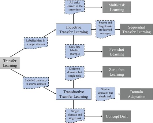
In what follows, we analyse each sub-paradigm of figure A1.

A.2. Transfer learning: sub-paradigms

Inductive Transfer Learning: It refers to the cases where labelled data is available in the target domain; in another sense, we have the typical Supervised learning scenario across the different domains and tasks. In inductive transfer methods, the target-task inductive bias is chosen or adjusted based on the source-task knowledge. The way this is done varies depending on which inductive learning algorithm is used to learn the source and target tasks (Torrey and Shavlik 2010). The main variations occur on how this learning is performed: simultaneously across source and target tasks (Multi-Task); sequentially by sampling source tasks, and updating the target task model (Sequential Transfer); and with the constraints of using only few labelled examples (Few-shot). We outline each variation:

• Multi-task Learning (Caruana 1997, Zhang and Yang 2017) is an approach to inductive transfer that improves generalization by learning tasks in parallel while using a shared representation; hence, ${\mathbb{P}}_T\left(Y_T|X_T\right)$ and ${\mathbb{P}}_S\left(Y_S|X_S\right)$ are intertwined, with the update in the target task affecting the behaviour of the domain tasks and vice versa. In practice, the learned model architecture and parameters are fully shared across domain and target tasks—inputs, weights or coefficients, transfer functions, and objective function. In finance, this mode of learning has been first used for stock selection (Ghosn and Bengio 1997); lately, it has been applied for day trading (Bitvai and Cohn 2015) and yield curves (Nunes et al. 2019).

• Sequential Transfer Learning (Ruder et al. 2019) is an approach to inductive transfer that improves generalization by learning tasks in sequence while using a shared representation to a certain extent; therefore, ${\mathbb{P}}_T\left(Y_T|X_T\right)$ and ${\mathbb{P}}_S\left(Y_S|X_S\right)$ are not completely intertwined, but the update in the target task impacts the behaviour of the domain tasks, and vice versa. In practice, the learned model architecture and parameters are partially shared across domain and target tasks—often weights, transfer functions, and sometimes the objective function. By not having to share the same inputs and other parts of the architecture, this mode of learning can be applied across different domains and make the learned model easier to reuse in future tasks. In the context of financial applications, it has been mainly applied for sentiment analysis: one of such applications is FinBERT (Araci 2019), a variation of BERT (Devlin et al. 2018b) specialized to financial sentiment analysis; it has obtained state-of-the-art results on FiQA sentiment scoring and Financial PhraseBank benchmarks. Hiew et al. (2019) provide a similar application but feeding the sentiment analysis index generated by BERT in an LSTM-based trading strategy to predict stock returns.

• Few-shot Learning (Fei-Fei et al. 2006, Goodfellow et al. 2016, Wang et al. 2019): It is an extreme form of inductive learning, with very few examples (sometimes only one) being used to learn the target task model. This works to the extent that the factors of variation corresponding to these invariances have been cleanly separated from the other factors, in the learned representation space, and that we have somehow learned which factors do and do not matter when discriminating objects of certain categories. During the transfer learning stage, only a few labelled examples are needed to infer the label of many possible test examples that all cluster around the same point in representation space. So far we were unable to find any application in finance that covers this paradigm. However, we believe that such a mode of learning can be applied for fraud detection, stock price forecasting that has recently undergone initial public offering, or any other situation where limited amount of data is present about the target task.

Transductive Transfer Learning: It refers to the cases where labelled data is only available in the source domain, although our objective is still to solve the target task; hence, we have a situation that is somewhat similar to what is known as Semi-supervised learning. What makes the transductive transfer methods feasible is the fact that the source and target tasks are the same, although the domains can be different. For example, consider the task of sentiment analysis, which consists of determining whether a comment expresses positive or negative sentiment. Comments posted on the web come from many categories. A transductive sentiment predictor trained on customer reviews of media content, such as books, videos and music, can be later used to analyse comments about consumer electronics, such as televisions or smartphones. There are three main forms of transductive transfer learning: Domain Adaptation, Concept Drift and Zero-shot learning. Each form is presented below:

• Domain Adaptation (Kouw and Loog 2019): In this case the tasks remain the same between each setting, but the domains as well as the input distribution are usually slightly different; therefore ${\mathcal{X}}_S\approx {\mathcal{X}}_T$ or ${\mathbb{P}}_T\left(X_T\right)\approx {\mathbb{P}}_S\left(X_S\right)$. The previous example of the sentiment predictor is a typical case, where the domains and the input distribution are somewhat different (books, videos and music reviews transferring to consumer electronics). We can presume that there is an underlying mapping that matches a certain statement to positive, neutral or negative sentiment, and what makes the problem harder to solve is the fact that the vocabulary and context vary between domains. Surprisingly simple unsupervised pretraining has been found to be very successful for sentiment analysis with domain adaptation (Glorot et al. 2011). Similarly to few-shot learning, this particular subarea of transfer learning has received less attention from the finance community, since most of the sentiment analysis and similar applications are handled using labelled data.

• Concept Drift (Žliobaitė et al. 2016, Escovedo et al. 2018): In this case the tasks and domains remain the same across settings, but the input distribution can gradually or abruptly change between them; therefore ${\mathbb{P}}_T\left(X_T\right)\ne {\mathbb{P}}_S\left(X_S\right)$. Often concept drift modelling and detection focus on continuous data streams, such as time series, text messages, videos, that is, data with a temporal dimension or indexation. Using the previous example, we would be concerned with changing views about a specific film: reviews that were otherwise extensively positive, gradually become negative due to changes in audience's view about how certain characters were portrayed, how the topic was approached, etc. This particular subarea has received substantial attention from the finance community: it has been used to discover relations between portfolio selection factors and stock returns (Hu et al. 2015); price forecasting (Liu et al. 2019); and fraud detection (Somasundaram and Reddy 2019).

• Zero-shot Learning (Socher et al. 2013, Wang et al. 2019) is a form of transductive transfer learning, where the domains and input distributions are different, and yet learning can be achieved by finding a suitable representation; hence ${\mathcal{X}}_S\ne {\mathcal{X}}_T$ and ${\mathbb{P}}_T\left(X_T\right)\ne {\mathbb{P}}_S\left(X_S\right)$. Following the previous example, if we have a database with thorough reviews about road bicycles, such as describing their frame, suspension, drivetrain, etc. It would be possible to learn in principle what constitutes a good or bad bicycle. Zero-shot learning would attempt to tap into this knowledge and transfer it to a new bicycle that we do not have reviews but use its design, 3d images, other descriptions, etc. to come up with an expected score, just based on users' opinions about the product. In this case, the task is the same (deciding the expected review of bicycle), but the domains are radically different (textual description versus an image). Similar to few-shot learning, we were unable to identify any piece of research from the finance community.

Also, there are four different approaches where the transference of knowledge from a task to another can be realized: instance, feature, parameters, and relational-knowledge. Table A3 presents a brief description, applications of each to the financial domain, and other key references. Undoubtedly, for financial applications parameter transfer is the preferred option, followed by instance transfer and feature transfer. Such approaches are mainly used for sentiment analysis, fraud detection, and forecasting, areas that have been widely researched using more traditional techniques. Conversely, we were unable to find research for relational knowledge. Despite that, we believe that researchers working on financial networks, peer-to-peer lending, etc. can benefit from methods in the relational-knowledge transfer approach.

Table D1. Approaches and applications of transfer learning across finance and general domains.

Approach	Brief description	Financial applications	Other references
Instance	Re-weighting labelled data in the source domain for use in the target domain	News-rich to news-poor stocks (Li et al. 2018); mitigating class imbalance in credit scoring (Li et al. 2018, Voumard and Beydoun 2019)	Jiang et al. (2019), Qu et al. (2019)
Feature	Find a suitable feature mapping to approximate the source domain to the target domain	Sentiment feature space (Li et al. 2018); Portfolio selection factors (Hu et al. 2015)	Zhuang et al. (2015), Yang et al. (2018)
Parameter	Learn shareable parameters or priors between the source and target tasks models	BERT specialized to financial sentiment analysis (Araci 2019, Hiew et al. 2019); Stock selection, forecasting (Ghosn and Bengio 1997, Bitvai and Cohn 2015); yield curve forecasting (Nunes et al. 2019)	Devlin et al. (2018b), Chen et al. (2019)
Relational-knowledge	Learn a logical relationship or rules in the source domain and transfer it to the target domain		Park et al. (2019), Wang et al. (2016)

Using this taxonomy, QuantNet can be classified as part of Sequential Transfer Learning, using a Parameter-transfer approach. In this sense, we aim to learn the target task model by sharing and updating the architecture's weights and activation functions across the tasks. Since each task has different number of inputs/outputs, this component is task specific. All of these details are better outlined in the next section.

Appendix 5.

In-depth comparison: QuantNet and no transfer linear

Market-level analysis. Figures A2(a) and A2(b) outline the average SR and CR across the 58 markets, ordered by No Transfer strategy performance. In SR terms, QuantNet outperforms No Transfer in its top 5 markets and dominates the bottom 10 markets both in SR and CR terms. Finally, in 7 of the top 10 largest ones (RTY, SPX, KOSPI, etc., see table A1), QuantNet has also outperformed No Transfer.

Figure A2. Average Sharpe (a) and Calmar (b) ratios of QuantNet and No Transfer across 58 markets.

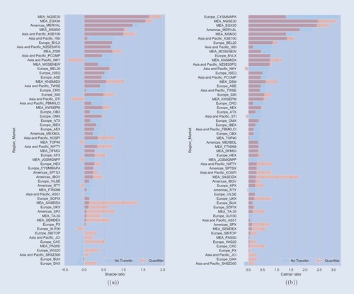
Figure A3 maps every market to a country and displays the relative outperformance (%) of QuantNet in relation to No Transfer in SR values. In the Americas, apart from Mexico and Argentina, Brazil, the USA (on average) and Canada, QuantNet has produced better results than No Transfer. Similarly, the core of Europe (Germany, the UK, and France), and India and China, QuantNet has produced superior SRs than No Transfer, with markets like Japan, Australia, New Zealand, and South Africa representing the reverse.

Figure A3. World map of average relative (%) Sharpe ratio difference between QuantNet versus No Transfer. For visualisation purposes, we have averaged the metric for the USA, China, and Israel/Palestine.

In a similar fashion to the global analysis, figures A4(a) and A4(b) display the relationship between SRs and CRs of No Transfer with QuantNet for each market, with overlaid regression curves. The SR and CR models have the following parameters: SR intercept of 0.1506 (p-value = 0.036), SR slope of 0.7381 (p-value < 0.0001); CR intercept of 0.1851 (p-value = 0.015), and CR slope of 0.7379 (p-value < 0.0001). Both cases indicate that in a market where No Transfer fared an SR or CR equal to 0, we would expect No Transfer to obtain on average 0.15 and 0.18 of SR and CR, respectively. Since both models have slope <1.0, it indicates that across markets QuantNet will tend to provide less surprisingly positive and negative SRs and CRs.

Figure A4. Scatterplot of QuantNet and No Transfer average Sharpe (a) and Calmar (b) ratios of each market overlaid by a linear regression curve.

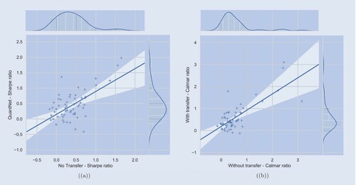
Table A4 presents a breakdown of the statistics in a few big regional markets, such as United States S&P 500 components (SPX Index), United Kingdom FTSE 100 (UKX Index), Korea Composite Index (KOSPI Index), and Saudi Arabia Tadawul All Shares (SASEIDX Index). Each one of them show 2–10 times order of magnitude improvement in SRs and CRs by QuantNet, with similar benefits in Sortino ratios, Downside risks, and Skewness.

Table E1. Financial metrics of QuantNet and No Transfer strategies in SPX Index, UKX Index, KOSPI Index, and SASEIDX Index.

	Americas_SPX		Asia and Pacific_KOSPI		Europe_UKX		MEA_SASEIDX
Mean (SD)	No transfer	QuantNet	No transfer	QuantNet	No transfer	QuantNet	No transfer	QuantNet
Ann Ret	0.000133	0.041031	0.073337	0.054152	0.000406	0.006555	0.000642	0.026092
	(0.001259)	(0.029839)	(0.25494)	(0.046237)	(0.001395)	(0.00609)	(0.002784)	(0.012866)
Ann Vol	0.002436	0.053368	0.403113	0.07075	0.002717	0.009576	0.003598	0.01895
	(0.00064)	(0.012918)	(0.144194)	(0.025008)	(0.00111)	(0.004583)	(0.003219)	(0.004739)
CR	0.133073	0.756976	0.289853	0.822309	0.210127	0.813796	0.267246	1.783155
	(0.377186)	(0.616175)	(0.620299)	(0.785171)	(0.445449)	(0.708568)	(0.745929)	(1.133185)
DownRisk	0.001717	0.035575	0.271677	0.047184	0.001661	0.005364	0.002236	0.010502
	(0.000522)	(0.009612)	(0.098263)	(0.017854)	(0.000433)	(0.002129)	(0.000513)	(0.002464)
Kurt	33.29913	19.51515	13.87472	22.58056	95.31436	88.42658	41.8963	33.41796
	(45.57039)	(18.51033)	(19.28247)	(34.13021)	(135.1503)	(116.5215)	(87.54653)	(48.08607)
MDD	−0.00467	−0.06681	−0.50323	−0.09328	−0.00432	−0.00988	−0.00614	−0.01755
	(0.002296)	(0.028684)	(0.190464)	(0.051306)	(0.001905)	(0.005301)	(0.003198)	(0.007012)
SR	0.061702	0.783197	0.347892	0.783428	0.108635	0.627227	0.12883	1.362307
	(0.512651)	(0.49204)	(0.540274)	(0.578968)	(0.529708)	(0.486396)	(0.579286)	(0.586632)
Skew	−0.21186	0.28355	0.374017	0.277958	2.943023	3.573138	0.495534	2.469297
	(2.851112)	(1.685894)	(1.36364)	(2.239952)	(6.586847)	(5.566353)	(4.07845)	(2.360219)
SortR	0.144905	1.245084	0.564466	1.256064	0.301707	1.207481	0.359786	2.587949
	(0.760463)	(0.847215)	(0.839065)	(0.979779)	(0.898402)	(0.979499)	(1.206481)	(1.344404)
	Americas_SPX		Asia and Pacific_KOSPI		Europe_UKX		MEA_SASEIDX
Median (MAD)	No transfer	QuantNet	No transfer	QuantNet	No transfer	QuantNet	No transfer	QuantNet
Ann Ret	0.000197	0.038476	0.059234	0.052772	0.000326	0.005321	0.000508	0.023614
	(0.000982)	(0.023214)	(0.188703)	(0.036438)	(0.00108)	(0.004778)	(0.001666)	(0.009858)
Ann Vol	0.002399	0.053732	0.380229	0.066449	0.002495	0.008573	0.003128	0.01865
	(0.000497)	(0.010269)	(0.111283)	(0.01968)	(0.000695)	(0.003598)	(0.001038)	(0.002928)
CR	0.045842	0.626018	0.133249	0.657845	0.092861	0.654498	0.091411	1.676411
	(0.271252)	(0.479759)	(0.470007)	(0.605487)	(0.328843)	(0.584447)	(0.410032)	(0.912643)
DownRisk	0.001648	0.035679	0.254761	0.044209	0.00157	0.004724	0.002257	0.009973
	(0.000395)	(0.007424)	(0.076679)	(0.013787)	(0.000333)	(0.00173)	(0.000405)	(0.001975)
Kurt	20.43113	14.44403	8.225536	13.04102	35.86203	30.40254	25.0625	28.02965
	(23.64829)	(10.23454)	(10.6417)	(17.31602)	(96.22141)	(86.32176)	(30.82765)	(15.90609)
MDD	−0.00419	−0.06071	-0.49819	−0.08132	−0.00393	−0.00841	−0.00578	−0.01573
	(0.001741)	(0.020741)	(0.157264)	(0.039347)	(0.001549)	(0.003937)	(0.002449)	(0.005458)
SR	0.085695	0.79579	0.366404	0.818361	0.154884	0.628875	0.184811	1.382302
	(0.406313)	(0.400688)	(0.437163)	(0.465154)	(0.407551)	(0.379645)	(0.451943)	(0.4808)
Skew	0.044563	0.407357	0.271776	0.148158	0.360259	1.385536	−0.06615	2.559821
	(1.742953)	(1.110312)	(0.811512)	(1.318841)	(4.960393)	(4.198536)	(2.102935)	(1.412129)
SortR	0.112332	1.205009	0.55375	1.235756	0.203793	1.128096	0.26026	2.315208
	(0.595473)	(0.690404)	(0.675314)	(0.779847)	(0.701329)	(0.793781)	(0.764835)	(1.124332)

These results by QuantNet also translate in superior cumulative returns ( figure A5), histograms with empirical distributions that stochastically dominate the No Transfer strategy ( figure A6), and finally positive transfer across assets ( figure A7). In summary, markets that were otherwise not as profit-generating using only lagged information become profitable due to the addition of a transfer layer of information across world markets.

Figure A5. Average cumulative returns (%) of SPX Index, UKX Index, KOSPI Index and SASEIDX Index contrasting QuantNet and No Transfer strategies. Before aggregation, each underlying asset was volatility-weighted to 10%.

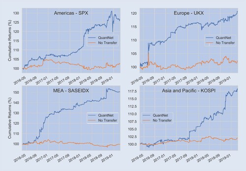
Figure A6. Histogram of Sharpe ratio of SPX Index, UKX Index, KOSPI Index, and SASEIDX Index contrasting QuantNet and No Transfer strategies.

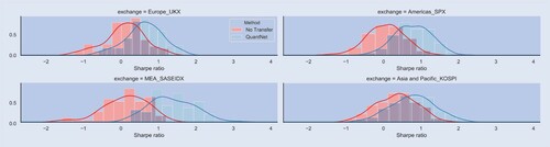
Figure A7. Scatterplot of Sharpe ratio of SPX Index, UKX Index, KOSPI Index, and SASEIDX Index contrasting QuantNet and No Transfer strategies.

Appendix 6.

Fama-French 5 factor model

We fit a traditional Fama-French 5 factor model, with the addition of Momentum factor (French 2012, Fama and French 2015) using these four markets daily returns as dependent variables. Table A5 presents the models coefficients, t-stats and whether they were or not statistically significant (using a 5% significance level). Regardless of the market, QuantNet provided significant alpha (abnormal risk-adjusted return) with very low correlation to other general market factors.

Table F1. Models coefficients and t-stats for the different markets and factors.

	SPX		UKX		SASEIDX		KOSPI
	Coefficient	t-stat	Coefficient	t-stat	Coefficient	t-stat	Coefficient	t-stat
Alpha	0.0003${}^{\ast }$	2.554	0.0002${}^{\ast }$	2.258	0.0006${}^{\ast }$	3.856	0.0003${}^{\ast }$	4.034
Beta	−0.0004${}^{\ast }$	−2.367	−0.0002	−1.558	−0.0006${}^{\ast }$	−2.804	−0.0001	−0.213
Small minus Big	0.0003	1.158	0.0002	1.075	0.0006	1.856	0.0001	0.182
High minus Low	−0.0005	−1.778	−0.0006${}^{\ast }$	−2.813	−0.0002	−0.781	−0.0001	−0.148
Momentum	−0.0002	−1.042	0.0001	0.08	−0.0002	−0.918	−0.0001	−0.538

${}^{\ast }$p-value < 0.05.

Appendix 7.

Dendrogram

An additional analysis is how each market is being mapped inside QuantNet architecture, particularly in the Encoder layer. The key question is how they are being represented in this hidden latent space and how close each market is to the other there. Figure A8 presents a dendrogram of hierarchical clustering done using the scores from encoder layer for all markets.

Figure A8. Dendrogram of hierarchical clustering using the scores from QuantNet encoder layer.

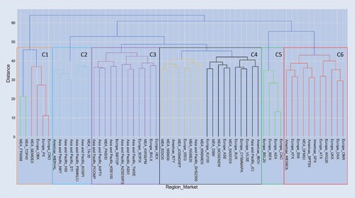
By setting an unique threshold across the hierarchical clustering we can form six distinct groups. Some clusters are easier to analyse, such as C5 that consist mainly of small European equity markets (Spain, Netherlands, Belgium, and France)—all neighbours; C6 comprising mainly of developed markets in Europe and Americas, such as the UK, Germany, the USA, and their respective neighbours Austria, Poland, Switzerland, Sweden, Denmark, Canada, and Mexico. Some clusters require a more refined observation, such as C2 containing most developed markets in Asia like Japan, Hong Kong, Korea, and Singapore, with C3 representing Asia and Pacific emerging markets: China, India, and some respective neighbours (Pakistan, Philippines, Taiwan).

Appendix 8.

Ablation study and sensitivity analysis

This section attempts to addresses the question: (i) could we get better results for the No Transfer strategy and (ii) what are the impact in QuantNet architecture by increasing its dimensionality, and performing some ablation in its architecture. Table A6 presents the Sharpe ratio (SR) statistics for question (i) and (ii), by contrasting QuantNet and No Transfer strategies.

Table H1. Average Sharpe ratio per different dimensions and configurations of QuantNet and No Transfer strategies.

		No transfer		QuantNet (encoder/decoder-transfer layer)
Sharpe ratio	Dimension	Linear	LSTM	Linear–Linear	Linear–LSTM	LSTM–Linear	LSTM–LSTM
Mean (SD)	10	0.324257	0.311424	0.355600	0.361986	0.370918	0.279758
		(0.6541)	(0.665251)	(0.704641)	(0.711988)	(0.715636)	(0.70962)
	25	0.324257	0.311424	0.333565	0.324842	0.325667	0.275786
		(0.6541)	(0.665251)	(0.702325)	(0.755392)	(0.707544)	(0.699151)
	50	0.324257	0.311424	0.319009	0.320583	0.234741	0.258272
		(0.6541)	(0.665251)	(0.698568)	(0.725952)	(0.752143)	(0.706733)
	100	0.324257	0.311424	0.326090	0.353448	0.228464	0.298445
		(0.6541)	(0.665251)	(0.695066)	(0.730362)	(0.722084)	(0.702126)
Median (MAD)	10	0.306572	0.304244	0.338981	0.345072	0.354776	0.275548
		(0.51182)	(0.515521)	(0.559216)	(0.533789)	(0.572184)	(0.562)
	25	0.306572	0.304244	0.314084	0.301769	0.273791	0.227461
		(0.51182)	(0.515521)	(0.552154)	(0.570677)	(0.555298)	(0.552615)
	50	0.306572	0.304244	0.302167	0.303684	0.205637	0.219550
		(0.51182)	(0.515521)	(0.546099)	(0.537824)	(0.583648)	(0.554146)
	100	0.306572	0.304244	0.307922	0.330039	0.188830	0.243308
		(0.51182)	(0.515521)	(0.540111)	(0.549627)	(0.573707)	(0.557717)

In relation to No Transfer, we can perceive that there is no benefit from moving to an LSTM architecture—in fact, we produced slightly worst outcomes in general. Maybe the lack of data per market has impacted the overall performance of this architecture. Similarly with QuantNet, a full LSTM model generated worst outcomes regardless of the dimensionality used. Linear components in QuantNet have produced better outcomes, with Linear encoders/decoders and LSTM transfer layers providing the best average results across dimensions. However, small layer sizes are linked with better SRs, and particularly for size equal to 10, the QuantNet architecture using LSTM encoders/decoders and Linear transfer layer generated the best average SRs.

Appendix 9.

Code

QuantNet and other strategies implementations can be found in this repository: https://www.dropbox.com/sh/k7g17x5razzxxdp/AABemBvG8UI99hp14z0C8fHZa?dl=0https://www.dropbox.com/sh/k7g17x5razzxxdp/AABemBvG8UI99hp14z0C8fHZa?dl=0

References

- Acar, E. and Satchell, S., Advanced Trading Rules, 2002 (Butterworth-Heinemann).
- Aggarwal, S. and Aggarwal, S., Deep investment in financial markets using deep learning models. Int. J. Comput. Appl., 2017, 162(2), 40–43.
- Allendbridge IS, Quantitative investment strategy survey. Pensions & Investments, 2014.
- Araci, D., Finbert: Financial sentiment analysis with pre-trained language models. Preprint, 2019. Available online at: arXiv:1908.10063.
- Avramovic, A., Lin, V. and Krishnan, M., We're all high frequency traders now. Credit Suisse Market Structure White Paper, 2017.
- Bailey, D.H. and Lopez de Prado, M., The Sharpe ratio efficient frontier. J. Risk, 2012, 15(2), 13.
- Baltzer, M., Jank, S. and Smajlbegovic, E., Who trades on momentum? J. Financ. Mark., 2019, 42, 56–74.
- BarclayHedge, Barclayhedge: CTA's asset under management, 2017. Available online at: https://www.barclayhedge.com/research/indices/cta/Money_Under_Management.html.
- Baxter, J., Learning internal representations. In Proceedings of the Eighth Annual Conference on Computational Learning Theory, pp. 311–320, 1995.
- Bayer, C., Horvath, B., Muguruza, A., Stemper, B. and Tomas, M., On deep calibration of (rough) stochastic volatility models. Preprint, 2019. Available online at: arXiv:1908.08806.
- Baz, J., Granger, N., Harvey, C.R., Le Roux, N. and Rattray, S., Dissecting investment strategies in the cross section and time series, 2015. Available online at: SSRN 2695101.
- Bengio, Y., Using a financial training criterion rather than a prediction criterion. Int. J. Neural Syst., 1997, 8(04), 433–443.
- Bergstra, J. and Bengio, Y., Random search for hyper-parameter optimization. J. Mach. Learn. Res., 2012, 13, 281–305.
- Bitvai, Z. and Cohn, T., Day trading profit maximization with multi-task learning and technical analysis. Mach. Learn., 2015, 101(1-3), 187–209.
- Blumberg, S.B., Tanno, R., Kokkinos, I. and Alexander, D.C., Deeper image quality transfer: Training low-memory neural networks for 3D images. In International Conference on Medical Image Computing and Computer-Assisted Intervention, pp. 118–125, 2018 (Springer).
- Blumberg, S.B., Palombo, M., Khoo, C.S., Tax, C.M.W., Tanno, R. and Alexander, D.C., Multi-stage prediction networks for data harmonization. In Medical Image Computing and Computer Assisted Intervention, pp. 411–419, 2019.
- Buehler, H., Gonon, L., Teichmann, J. and Wood, B., Deep hedging. Quant. Finance, 2019, 19(8), 1271–1291.
- Caruana, R., Multitask learning: A knowledge-based source of inductive bias. In Proceedings of the Tenth International Conference on Machine Learning, pp. 41–48, 1993 (Morgan Kaufmann).
- Caruana, R., Multitask learning. Mach. Learn., 1997, 28(1), 41–75.
- Chen, S., Ma, K. and Zheng, Y., Med3D: Transfer learning for 3D medical image analysis. Preprint, 2019. Available online at: arXiv:1904.00625.
- Cho, K., van Merriënboer, B., Gulcehre, C., Bahdanau, D., Bougares, F., Schwenk, H. and Bengio, Y., Learning phrase representations using RNN encoder–decoder for statistical machine translation. In Proceedings of the 2014 Conference on Empirical Methods in Natural Language Processing (EMNLP), pp. 1724–1734, 2014a.
- Cho, K., van Merrienboer, B., Bahdanau, D. and Bengio, Y., On the properties of neural machine translation: Encoder–decoder approaches, CoRR, 2014b. Available online at: http://arxiv.org/abs/1409.1259.
- Choueifaty, Y. and Coignard, Y., Toward maximum diversification. J. Portf. Manag., 2008, 35(1), 40–51.
- Daniel, K. and Moskowitz, T.J., Momentum crashes. J. Financ. Econ., 2016, 122(2), 221–247.
- De Prado, M.L., Advances in Financial Machine Learning, 2018 (John Wiley & Sons).
- Devlin, J., Chang, M.-W., Lee, K. and Toutanova, K., Bert: Pre-training of deep bidirectional transformers for language understanding. Preprint, 2018a. Available online at: arXiv:1810.04805.
- Devlin, J., Chang, M.-W., Lee, K. and Toutanova, K., Bert: Pre-training of deep bidirectional transformers for language understanding. Preprint, 2018b. Available online at: arXiv:1810.04805.
- Dichtl, H., Investing in the S&P 500 index: Can anything beat the buy-and-hold strategy. Rev. Financ. Econ., 2020, 38(2), 352–378.
- Du Plessis, J. and Hallerbach, W.G., Volatility weighting applied to momentum strategies. J. Altern. Invest., 2016, 19(3), 40–58.
- El Bsat, S., Ammar, H.B. and Taylor, M.E., Scalable multitask policy gradient reinforcement learning. In Thirty-First AAAI Conference on Artificial Intelligence, 2017.
- Eling, M. and Schuhmacher, F., Does the choice of performance measure influence the evaluation of hedge funds. J. Bank. Finance, 2007, 31(9), 2632–2647.
- Elton, E.J., Gruber, M.J. and de Souza, A., Passive mutual funds and ETFs: Performance and comparison. J. Bank. Finance, 2019, 106, 265–275.
- Escovedo, T., Koshiyama, A., da Cruz, A.A. and Vellasco, M., Detecta: Abrupt concept drift detection in non-stationary environments. Appl. Soft Comput., 2018, 62, 119–133.
- Fama, E.F. and French, K.R., A five-factor asset pricing model. J. Financ. Econ., 2015, 116(1), 1–22.
- Fei-Fei, L., Fergus, R. and Perona, P., One-shot learning of object categories. IEEE Trans. Pattern Anal. Mach. Intell., 2006, 28(4), 594–611.
- Feng, G., Giglio, S. and Xiu, D., Taming the factor zoo: A test of new factors. J. Finance, 2020, 75(3), 1327–1370.
- Firoozye, N. and Koshiyama, A., Optimal dynamic strategies on gaussian returns, 2019. Available online at: SSRN 3385639.
- Fischer, T. and Krauss, C., Deep learning with long short-term memory networks for financial market predictions. Eur. J. Oper. Res., 2018, 270(2), 654–669.
- Flennerhag, S., Yin, H., Keane, J. and Elliot, M., Breaking the activation function bottleneck through adaptive parameterization. In Advances in Neural Information Processing Systems, pp. 7739–7750, 2018.
- Flennerhag, S., Rusu, A.A., Pascanu, R., Visin, F., Yin, H. and Hadsell, R., Meta-learning with warped gradient descent. In International Conference on Learning Representations, 2020a.
- Flennerhag, S., Rusu, A.A., Pascanu, R., Visin, F., Yin, H. and Hadsell, R., Meta-learning with warped gradient descent. In International Conference on Learning Representations, 2020b.
- French, K.R., Kenneth R. French-data library. Tuck-MBA Program Web Server, 2012. Available online at: http://mba.tuck.dartmouth.edu/pages/faculty/ken.french/data_library.html (accessed 20 October 2010).
- Gao, Z., Gao, Y., Hu, Y., Jiang, Z. and Su, J., Application of deep q-network in portfolio management. Preprint, 2020. Available online at: arXiv:2003.06365.
- Gers, F.A., Schmidhuber, J. and Cummins, F., Learning to forget: Continual prediction with LSTM, 1999.
- Ghosn, J. and Bengio, Y., Multi-task learning for stock selection. In Advances in Neural Information Processing Systems, pp. 946–952, 1997.
- Gibiansky, A., Arik, S., Diamos, G., Miller, J., Peng, K., Ping, W., Raiman, J. and Zhou, Y., Deep voice 2: Multi-speaker neural text-to-speech. In Advances in Neural Information Processing Systems, pp. 2962–2970, 2017.
- Glorot, X., Bordes, A. and Bengio, Y., Domain adaptation for large-scale sentiment classification: A deep learning approach. In Proceedings of the 28th International Conference on Machine Learning (ICML-11), pp. 513–520, 2011.
- Goodfellow, I., Bengio, Y. and Courville, A., Deep Learning, 2016 (MIT Press).
- Gu, S., Kelly, B. and Xiu, D., Empirical asset pricing via machine learning. Rev. Financ. Stud., 2020, 33(5), 2223–2273.
- Harvey, C.R. and Liu, Y., Backtesting. J. Portf. Manag., 12–28.
- He, X., Alesiani, F. and Shaker, A., Efficient and scalable multi-task regression on massive number of tasks. In Proceedings of the AAAI Conference on Artificial Intelligence, Vol. 33, pp. 3763–3770, 2019.
- Heaton, J.B., Polson, N.G. and Witte, J.H., Deep learning for finance: Deep portfolios. Appl. Stoch. Models Bus. Ind., 2017, 33(1), 3–12.
- Hiew, J.Z.G., Huang, X., Mou, H., Li, D., Wu, Q. and Xu, Y., Bert-based financial sentiment index and LSTM-based stock return predictability. Preprint, 2019. Available online at: arXiv:1906.09024.
- Hochreiter, S. and Schmidhuber, J., Long short-term memory. Neural Comput., 1997, 9(8), 1735–1780.
- Hu, Y., Liu, K., Zhang, X., Xie, K., Chen, W., Zeng, Y. and Liu, M., Concept drift mining of portfolio selection factors in stock market. Electron. Commer. Res. Appl., 2015, 14(6), 444–455.
- Jegadeesh, N. and Titman, S., Returns to buying winners and selling losers: Implications for stock market efficiency. J. Finance, 1993, 48(1), 65–91.
- Jeong, G. and Kim, H.Y., Improving financial trading decisions using deep q-learning: Predicting the number of shares, action strategies, and transfer learning. Expert Syst. Appl., 2019, 117, 125–138.
- Jiang, S., Mao, H., Ding, Z. and Fu, Y., Deep decision tree transfer boosting. IEEE Trans. Neural Netw. Learn. Syst., 2019.
- Kenett, D.Y., Raddant, M., Zatlavi, L., Lux, T. and Ben-Jacob, E., Correlations and dependencies in the global financial village. In International Journal of Modern Physics: Conference Series, Vol. 16, pp. 13–28, 2012 (World Scientific).
- Kornblith, S., Shlens, J. and Le, Q.V., Do better imagenet models transfer better? In Proceedings of the IEEE Conference on Computer Vision and Pattern Recognition, pp. 2661–2671, 2019.
- Koshiyama, A. and Firoozye, N., Avoiding backtesting overfitting by covariance-penalties: An empirical investigation of the ordinary and total least squares cases. J. Financ. Data Sci., 2019a, 1(4), 63–83.
- Koshiyama, A. and Firoozye, N., Avoiding backtesting overfitting by covariance-penalties: An empirical investigation of the ordinary and total least squares cases. J. Financ. Data Sci., 2019b, 1(4), 63–83.
- Kouw, W.M. and Loog, M., A review of domain adaptation without target labels. IEEE Trans. Pattern Anal. Mach. Intell., 2019.
- Lee, Y. and Choi, S., Gradient-based meta-learning with learned layerwise metric and subspace. Preprint, 2018. Available online at: arXiv:1801.05558.
- Lee, C.-Y., Xie, S., Gallagher, P., Zhang, Z. and Tu, Z., Deeply-supervised nets. In International Conference on Artificial Intelligence and Statistics, 2015.
- Li, W., Ding, S., Chen, Y. and Yang, S., A transfer learning approach for credit scoring. In International Conference on Applications and Techniques in Cyber Security and Intelligence, pp. 64–73, 2018 (Springer).
- Li, X., Xie, H., Lau, R.Y., Wong, T.-L. and Wang, F.-L., Stock prediction via sentimental transfer learning. IEEE Access, 2018, 6, 73110–73118.
- Li, Y., Ni, P. and Chang, V., Application of deep reinforcement learning in stock trading strategies and stock forecasting. Computing, 2019, 1–18.
- Lim, B., Zohren, S. and Roberts, S., Enhancing time-series momentum strategies using deep neural networks. J. Financ. Data Sci., 2019, 1(4), 19–38.
- Liu, Z., Loo, C.K. and Seera, M., Meta-cognitive recurrent recursive kernel OS-ELM for concept drift handling. Appl. Soft Comput., 2019, 75, 494–507.
- Liu, Y., Ott, M., Goyal, N., Du, J., Joshi, M., Chen, D., Levy, O., Lewis, M., Zettlemoyer, L. and Stoyanov, V., Roberta: A robustly optimized bert pre-training approach. Preprint, 2019. Available online at: arXiv:1907.11692.
- Lu, D.W., Agent inspired trading using recurrent reinforcement learning and LSTM neural networks. Preprint, 2017. Available online at: arXiv:1707.07338.
- Martellini, L., Toward the design of better equity benchmarks: Rehabilitating the tangency portfolio from modern portfolio theory. J. Portf. Manag., 2008, 34(4), 34–41.
- Mikolov, T., Sutskever, I., Chen, K., Corrado, G.S. and Dean, J., Distributed representations of words and phrases and their compositionality. In Advances in Neural Information Processing Systems, pp. 3111–3119, 2013.
- Molyboga, M., Portfolio management of commodity trading advisors with volatility targeting, 2018. Available online at: SSRN 3123092.
- Moskowitz, T.J., Ooi, Y.H. and Pedersen, L.H., Time series momentum. J. Financ. Econ., 2012, 104(2), 228–250.
- Nunes, M., Gerding, E., McGroarty, F. and Niranjan, M., A comparison of multitask and single task learning with artificial neural networks for yield curve forecasting. Expert Syst. Appl., 2019, 119, 362–375.
- Pan, S.J. and Yang, Q., A survey on transfer learning. IEEE Trans. Knowl. Data Eng., 2009, 22(10), 1345–1359.
- Park, W., Kim, D., Lu, Y. and Cho, M., Relational knowledge distillation. In The IEEE Conference on Computer Vision and Pattern Recognition (CVPR), 2019.
- Pendharkar, P.C. and Cusatis, P., Trading financial indices with reinforcement learning agents. Expert Syst. Appl., 2018, 103, 1–13.
- Qu, C., Ji, F., Qiu, M., Yang, L., Min, Z., Chen, H., Huang, J. and Croft, W.B., Learning to selectively transfer: Reinforced transfer learning for deep text matching. In Proceedings of the Twelfth ACM International Conference on Web Search and Data Mining, pp. 699–707, 2019 (ACM).
- Raddant, M. and Kenett, D.Y., Interconnectedness in the global financial market. OFR WP 16-09, 2016.
- Radford, A., Wu, J., Child, R., Luan, D., Amodei, D. and Sutskever, I., Language models are unsupervised multitask learners. OpenAI Blog, 2019, 1(8), 9.
- Reddi, S.J., Kale, S. and Kumar, S., On the convergence of ADAM and beyond. Preprint, 2019. Available online at: arXiv:1904.09237.
- Rollinger, T. and Hoffman, S., Sortino ratio: A better measure of risk. Futures Mag., 2013, 1(2).
- Romano, J.P. and Wolf, M., Stepwise multiple testing as formalized data snooping. Econometrica, 2005, 73(4), 1237–1282.
- Ruder, S., An overview of multi-task learning in deep neural networks. Preprint, 2017. Available online at: arXiv:1706.05098.
- Ruder, S., Peters, M.E., Swayamdipta, S. and Wolf, T., Transfer learning in natural language processing. In Proceedings of the 2019 Conference of the North American Chapter of the Association for Computational Linguistics: Tutorials, pp. 15–18, 2019.
- Sezer, O.B., Gudelek, M.U. and Ozbayoglu, A.M., Financial time series forecasting with deep learning: A systematic literature review: 2005–2019. Appl. Soft Comput., 2020, 90, 106181.
- Sharpe, W.F., The sharpe ratio. J. Portf. Manag., 1994, 21(1), 49–58.
- Socher, R., Ganjoo, M., Manning, C.D. and Ng, A., Zero-shot learning through cross-modal transfer. In Advances in Neural Information Processing Systems, pp. 935–943, 2013.
- Somasundaram, A. and Reddy, S., Parallel and incremental credit card fraud detection model to handle concept drift and data imbalance. Neural Comput. Appl., 2019, 31(1), 3–14.
- Sutskever, I., Training recurrent neural networks. PhD Thesis, CAN, 2013.
- Thomann, A., Factor-based tactical bond allocation and interest rate risk management, 2019. Available online at: SSRN 3122096.
- Torrey, L. and Shavlik, J., Transfer learning. In Handbook of Research on Machine Learning Applications and Trends: Algorithms, Methods, and Techniques, pp. 242–264, 2010 (IGI Global).
- Vargas, M.R., De Lima, B.S. and Evsukoff, A.G., Deep learning for stock market prediction from financial news articles. In 2017 IEEE International Conference on Computational Intelligence and Virtual Environments for Measurement Systems and Applications (CIVEMSA), pp. 60–65, 2017 (IEEE).
- Voit, J., The Statistical Mechanics of Financial Markets, 2013 (Springer Science & Business Media).
- Voumard, A. and Beydoun, G., Transfer learning in credit risk. In ECML PKDD, pp. 1–16, 2019.
- Wang, L., Lee, C.-Y., Tu, Z. and Lazebnik, S., Training deeper convolutional networks with deep supervision, 2015. Available online at: arXiv:1505.02496.
- Wang, D., Li, Y., Lin, Y. and Zhuang, Y., Relational knowledge transfer for zero-shot learning. In Proceedings of the Thirtieth AAAI Conference on Artificial Intelligence', AAAI'16, pp. 2145–2151, 2016 (AAAI Press). Available online at: http://dl.acm.org/citation.cfm?id=3016100.3016198.
- Wang, W., Zheng, V.W., Yu, H. and Miao, C., A survey of zero-shot learning: Settings, methods, and applications. ACM Trans. Intell. Syst. Technol., 2019, 10(2), 13.
- Wang, Y., Yao, Q., Kwok, J. and Ni, L.M., Generalizing from a few examples: A survey on few-shot learning, 2019.
- Yang, Z., Zhao, J., Dhingra, B., He, K., Cohen, W.W., Salakhutdinov, R.R. and LeCun, Y., GloMo: Unsupervised learning of transferable relational graphs. In Advances in Neural Information Processing Systems, pp. 8950–8961, 2018.
- Young, T.W., Calmar ratio: A smoother tool. Futures, 1991, 20(1), 40.
- Yu, S. and Principe, J.C., Understanding autoencoders with information theoretic concepts. Neural Netw., 2019, 117, 104–123.
- Zhang, L., Transfer adaptation learning: A decade survey. Preprint, 2019. Available online at: arXiv:1903.04687.
- Zhang, Y. and Yang, Q., A survey on multi-task learning. Preprint, 2017. Available online at: arXiv:1707.08114.
- Zhang, M., Jiang, X., Fang, Z., Zeng, Y. and Xu, K., High-order hidden Markov model for trend prediction in financial time series. Physica A, 2019, 517, 1–12.
- Zhang, Z., Zohren, S. and Roberts, S., Deep reinforcement learning for trading. J. Financ. Data Sci., 2020, 2(2), 25–40.
- Zhuang, F., Cheng, X., Luo, P., Pan, S.J. and He, Q., Supervised representation learning: Transfer learning with deep autoencoders. In Twenty-Fourth International Joint Conference on Artificial Intelligence, 2015.
- Zhuang, F., Qi, Z., Duan, K., Xi, D., Zhu, Y., Zhu, H., Xiong, H. and He, Q., A comprehensive survey on transfer learning. Preprint, 2019. Available online at: arXiv:1911.02685.
- Zintgraf, L.M., Shiarlis, K., Kurin, V., Hofmann, K. and Whiteson, S., Fast context adaptation via meta-learning. Preprint, 2018. Available online at: arXiv:1810.03642.
- Žliobaitė, I., Pechenizkiy, M. and Gama, J., An overview of concept drift applications. In Big Data Analysis: New Algorithms for a New Society, pp. 91–114, 2016 (Springer).
Appendix 1.
Datasets
Table presents the datasets/markets used to empirically evaluate QuantNet. All the data was obtained via Bloomberg, with the description of each market/index and its constituents at https://www.bloomberg.com; for instance, SPX can be found by searching using the following link: https://www.bloomberg.com/quote/SPX:IND. We tried to find a compromise between number of assets and sample size, hence for most markets we were unable to use the full list of constituents. We aimed to collect daily price data ranging from 03/01/2000 to 15/03/2019, but for most markets it starts roughly around 2010. Finally, due to restrictions from our Bloomberg license, we were unable to access data for some important equity markets, such as Italy and Russia. Full list with assets and respective exchange can be found at: https://www.dropbox.com/s/eobhg2w8ithbgsp/AssetsExchangeList.xlsx?dl=0