A generalized heterogeneous autoregressive model using market information

Abstract

This paper introduces a novel class of volatility forecasting models that incorporate market realized (co)variances and semi(co)variances within the framework of a heterogeneous autoregressive (HAR) model. Our empirical analysis shows statistically and economically significant forecasting gains. For our most parsimonious market-HAR specification, stock volatility forecasting is improved by 9.80% points. Using a mixed sampling frequency market-HAR variant with low (high) sampling frequency for the stock (market) improves forecasting by a further 6.90% points. Our paper also develops noise-robust estimators to facilitate the use of realized semi(co)variances at high sampling frequencies.

Keywords:

• Realized volatility
• Microstructure noise
• Pre-averaged estimators
• Semi-variance
• Semi-covariance
• Volatility forecasting

JEL Classifications:

• C22
• C51
• C58
• G11

1. Introduction

Comparing financial econometrics and asset pricing studies, Bollerslev (2022) argues that the former remains uninformed about the inherently multivariate issues in finance, such as covariation among multiple assets or systematic risk factors. This paper addresses this gap. We motivate and introduce a model for stock volatility that incorporates a market volatility factor. Our results show that stock volatility forecasting improves significantly, both in statistical and economic terms. Thus market volatility is a significant factor in modeling and forecasting stock volatility.

Asset pricing studies dating back to the model of Sharpe (1964), Lintner (1965) and Black et al. (1972) posit that the market factor is sufficient to explain the cross-section of expected returns. Empirical support for this claim has been futile. Instead, additional factors have been proposed ,¹ such as value and size (Fama and French 1993), momentum (Jegadeesh and Titman 1993), liquidity (Pástor and Stambaugh 2003), and market volatility (Ang et al. 2006b).² An interrelationship between asset return and volatility dates back to Fama and MacBeth (1973), Campbell and Hentschel (1992) and Glosten et al. (1993). However, the inclusion of market volatility as ‘a priced factor’ suggests that, determining their investment set, investors value both contemporaneous return and future return uncertainty (Campbell 1996, Chen 2002).

Unlike observed logarithmic returns, risk is latent. Noisy proxies for risk (e.g. squared returns) have been superseded by conditional variance estimators and stochastic volatility models. The advent of high-frequency data marked a paradigm shift in volatility modeling and forecasting.³ An efficient estimator of return volatility, the realized variance (RV), has been shown to dominate GARCH-type and stochastic volatility (SV) models (Andersen et al. 2003). Additionally, the simple and easy-to-estimate HAR model (Corsi 2009) has dominated other approaches for modeling and forecasting realized measures.⁴ Owing to the vastness of tick-level data and limits in computational power, the financial econometrics literature is largely univariate or small-scale multivariate.⁵ Put simply, individual stock volatility modeling and forecasting is agnostic about other stocks or indeed any systematic risk factors.

Our motivation is twofold: on the one hand, we argue that individual stock volatility modeling and forecasting should be informed by dynamics in other stocks or systematic risk factors. The market factor is the most commonly appearing in the asset pricing literature. Hence, it is not unreasonable to assume that a market volatility factor would have explanatory power for individual stock volatilities. Contrarily a case could be made when the market volatility factor would be uninformative. This would require that market wide uncertainties are timely and correctly incorporated within individual stock dynamics. We feel this is unrealistic for two reasons: first, an assumption of market efficiency is required (i.e. all available information is correctly reflected in the stock price) but unlikely to hold. Instead, it may take some time for financial analysts and/or traders to gauge the impact of news on individual stocks, as well as precisely trace the exact effect of a certain macroeconomic announcement (i.e. ‘soft’ news, see Bollerslev (2022)). Second, it assumes investor rationality while ignoring investor biases, technical analysis and algorithmic trading.

On the other hand, ever since the asset pricing literature has been using a timeseries regression, returns are bound to be outperformed by volatilities on informational content alone. In other words, a timeseries model at the daily horizon would explain a much larger fraction of stock volatility than stock return.⁶ Therefore, a timeseries volatility model in the spirit of asset pricing factor models has two key advantages: first, there is more informational content to be captured owing to the high persistence feature of the volatility process. Second, as the stock-specific autoregressive components of the HAR model capture a sizeable fraction of the variation in stock volatility, they leave less room for false factors essentially acting as a shield towards the ‘zoo’ of factors criticism. Our proposed model builds on the popular HAR framework for modeling stock volatility. To this we add market volatility and stock-market covariation information from realized measures. We call it the market-HAR. Being a univariate specification, it retains the key features of the HAR, namely its flexibility and estimation simplicity. Resembling the asset pricing models intuition, the market-HAR allows market information reflected in market-volatility to affect stock volatility. However, unlike asset pricing models that assume a constant relation between stock and market returns, the market-HAR allows it to vary across time.⁷ Put simply, market-volatility influence on stock volatility forecasting can be higher in specific periods, for instance during financial crisis. To capture this information, market-HAR incorporates realized covariance information between stock and market.

We generalize the market-HAR by (i) incorporating semi-variance and semi-covariance measures; (ii) allowing for different sampling frequencies between firm-specific and market-specific realized measures; and (iii) considering the impact of jumps. That disentangling good from bad volatility improves HAR forecasting performance is well documented (Patton and Sheppard 2015). In our market-HAR extensions, we use stock-specific and market-specific realized semi-variances (Barndorff-Nielsen et al. 2010) as well as their respective realized semi-covariances (Bollerslev et al. 2020). This enhances the capacity of market-HAR models to deal with asymmetries in volatilities and covariances, which is relevant for downside risk management (Grootveld and Hallerbach 1999, Ang et al. 2006a, Huang 2008, Guerard et al. 2013). Where realized semi-variances are segregated by their signed returns, realized semi-covariances are split in four components by their concordant and discordant signed returns.

We also consider a mixed sampling market-HAR variant that allows for different sampling frequencies between the firm-specific and market-specific components. To explore potential benefits over a wide range of frequencies, we mitigate the impact of market microstructure noise (MMSN) by the use of noise-robust realized variances (Jacod et al. 2009, Christensen et al. 2014) and noise-robust realized covariances (Christensen et al. 2010). We develop noise-robust realized semi-variance and semi-covariance measures by extending previous work in this area. Our modified noise-robust measures permit the use of realized measures at frequencies higher than the popular 300-second. Previous studies deliver improvements in forecasting when noise-robust measures are used in the presence of MMSN relative to standard volatility measures (Ghysels and Sinko 2011, Bu et al.2021).

Jumps are important in forecasting, with mixed evidence to the nature of their contribution (Giot and Laurent 2007, Andersen et al. 2007, Corsi et al. 2010, Busch et al. 2011, Patton and Sheppard 2015, Nolte and Xu 2015, Bu et al. 2021). To acknowledge the impact of jumps in our market-HAR model, we introduce individual jumps in the firm-specific and market-specific components, while we also account for the existence of co-jumps.

For the empirical analysis, intraday data for 20 NYSE stocks from 2000 to 2016 across a representative sample of business sectors are used. The SPDR (SPY) S&P 500 ETF acts as a proxy for the market factor over the same period. The main results are that the market-HAR model delivers significant improvements for in-sample and out-of-sample forecasting. As compared with the benchmark HAR model, the most parsimonious market-HAR model enhances individual stock volatility forecasting by 9.80% points on average for the 300-second, 1-day ahead horizon. In accounting for asymmetric effects, market-HAR models enhance forecasting performance by a further 8.40% points. Models that incorporate realized semi(co)variance information deliver superior volatility forecasting over their more parsimonious counterparts. These full-fledged market-HAR models improve volatility forecasting by up to 30.70% points relative to the benchmark HAR model. Forecasting performance is moderated at high sampling frequencies and/or long forecasting horizons. Yet the market-HAR models remain between 19.4 % and 20.9% points superior to the HAR without market information. A mixed sampling market-HAR model also increases forecasting performance when low (high) sampling frequencies of the stock (market) are combined. To underscore the practical relevance of the forecasting improvements of the market-HAR model, we evaluate gains in hypothetical portfolio allocation decisions. Relying on a utility-based framework (Fleming et al. 2001, 2003, Bernales and Guidolin 2014, Christoffersen et al. 2014, Nolte and Xu 2015) ignoring market information in volatility forecasting can raise the annual cost to risk-averse investors by up to 57 basis points.

Our study offers three contributions to the finance literature. First, we introduce a univariate model that allows for market-specific information to complement stock volatility modeling and forecasting. Second, we develop and utilize noise-robust measures of the realized semi-variances and semi-covariances to exploit the information content of realized measures across a wider range of sampling frequencies. Third, we conduct the first forecasting study using a mixture of sampling frequencies between the firm and market components. While the consensus is that market microstructure noise increases at higher sampling frequencies, our use of noise-robust measures allows us to better explore the informational content across these assets.

The remainder of the paper is organized as follows. Section 2 describes the theoretical background and the new noise-robust realized semi-variances and semi-covariances; Section 3 outlines the forecasting models and evaluation criteria, and sets out the economic value approach; Section 4 describes our data; Section 5 presents and discusses the empirical results. Section 6 reports a robustness exercise that includes the use of jumps and logarithmic transformation of the realized variances. Concluding remarks and directions for future research are provided in Section 7.

2. Theoretical background

We consider a factor-type log price process (Ng et al. 1992, Fan et al. 2016), defined on some filtered probability space $(\mathrm{\Omega },\mathcal{F},{\mathcal{F}}_{t\ge 0},\mathbb{P})$, evolving continuously over time: (1) $P_t=\text{β}{F}_t+Z_t,$(1) where $P_t$ is the log-price of an individual asset, $F_t$ is the K-dimensional factor process, $Z_t$ is the idiosyncratic component, and β is an $1\times K$ vector of constant factor loadings. To complete the specification, we make similar assumptions to those in Fan et al. (2016) on the dynamics of factors and idiosyncratic components.

Assumption 2.1

Suppose the log asset prices, $P_t$, follows a factor model given by equation (1(1) $P_t=\text{β}{F}_t+Z_t,$(1) ), in which $F_t$ and $Z_t$ are continuous Itô semimartingales: (2) $\begin{array}{rl}{F}_{t,k}& ={\int }_0^t{a}_{s,k}\mathrm{d}s+{\int }_0^t{\eta }_{s,k}\mathrm{d}{W}_{s,k},\end{array}$(2) (3) $\begin{array}{rl}{Z}_t& ={\int }_0^t{b}_s\mathrm{d}s+{\int }_0^t{\sigma }_s\mathrm{d}{B}_s,\end{array}$(3) where ${\eta }_{s,k}$ and ${\sigma }_s$ are the respective systematic and idiosyncratic spot volatilities, which are adapted and càdlàg, $W_{s,k}$ and $B_s$ are two Brownian motions. Whereas $W_{s,k}$ is independent of $B_s$, we allow for correlation among factors, that is $〈\mathrm{d}{W}_{s,l},\mathrm{d}{W}_{s,i}〉={\rho }_{s,l,i}\mathrm{d}s$ for $i\ne l$,⁸ where $〈\cdot ,\cdot 〉$ denotes the quadratic covariation. In addition, $a_{s,k}$ and $b_s$ are drift terms which are progressively measurable.

To facilitate the exposition, we consider the case of two main factors, the market factor, $F_m$, and a latent and relevant factor, $F_k$, which takes the following form: (4) $P_t={\text{β}}_m{F}_{t,m}+{\gamma }_k{F}_{t,k}+Z_t.$(4) Under assumption 2.1, we have that the integrated variance of $P_t$ is defined as (5) $\begin{array}{rl}〈P_t,P_t〉& =\underset{I{V}_t^s}{\underbrace{{\gamma }_k^2{\int }_0^t{\eta }_{s,k}^2\mathrm{d}s+{\int }_0^t{\sigma }_s^2\mathrm{d}s}}+\underset{I{V}_t^m}{\underbrace{{\text{β}}_m^2{\int }_0^t{\eta }_{s,m}^2\mathrm{d}s}}\\ & +\underset{ICO{V}_t}{\underbrace{{\text{β}}_m{\gamma }_k{\int }_0^t{\rho }_s{\eta }_{s,m}{\eta }_{s,k}\mathrm{d}s}}.\end{array}$(5) The above result suggests that the total integrated variance of an individual asset is related to three components⁹: idiosyncratic variance, systematic variances, and covariance component. One would expect that each of these components possesses value in a forecasting setting. In this spirit, we propose to model and forecast the asset variance by incorporating proxies for these elements separately in our market-HAR model specifications outlined in Section 3. However, the accurate estimation of idiosyncratic variance has been proven rather difficult in practice, where the literature has identified more than 300 factors that explain the cross-section of stock returns (Harvey et al. 2016), and yet the idiosyncratic variance comprises most of the total variance (Ang et al. 2009). Moreover, it is custom in the literature to use past total variance in HAR specifications. Given that from a regression point of view a model with past idiosyncratic and systematic variances is observationally equivalent (only regression parameter values would differ) to a model with total and systematic variances, we refrain from obtaining idiosyncratic variance and use common total variance instead, alongside the systematic variance and a covariation term.

The integrated variance and covariance outlined in equation (5(5) $\begin{array}{rl}〈P_t,P_t〉& =\underset{I{V}_t^s}{\underbrace{{\gamma }_k^2{\int }_0^t{\eta }_{s,k}^2\mathrm{d}s+{\int }_0^t{\sigma }_s^2\mathrm{d}s}}+\underset{I{V}_t^m}{\underbrace{{\text{β}}_m^2{\int }_0^t{\eta }_{s,m}^2\mathrm{d}s}}\\ & +\underset{ICO{V}_t}{\underbrace{{\text{β}}_m{\gamma }_k{\int }_0^t{\rho }_s{\eta }_{s,m}{\eta }_{s,k}\mathrm{d}s}}.\end{array}$(5) ) can be consistently estimated using the realized variance and covariance (Andersen et al. 2001a, 2003, Barndorff-Nielsen and Shephard 2004). However, these measures are not consistent estimates of the integrated variance and covariance when the observed price contains measurement error. Since, in practice, the observed price process is contaminated with microstructure noise (see Bandi and Russell 2006, Hansen and Lunde 2006 among others), in the next section we introduce realized measures that are robust to the presence of such contamination.

2.1. Realized measures and market microstructure noise

In the presence of market microstructure noise, the price is observed with a measurement error, which distorts the standard realized measures.¹⁰ In particular, the observed price is the sum of an unobservable efficient price and a noise component due to imperfections of the trading process: (6) $P_t^{\ast }=P_t+U_t,$(6) where $P_t^{\ast }$ is the contaminated price, $P_t$ is the efficient price, and $U_t$ is the observation error, which is independent and identically distributed with $\mathbb{E}\left[U_t\right]=0$ and $\mathbb{E}\left[U_t^2\right]={\omega }^2$, and $P_t\perp U_t$. The contaminated returns are estimated as $r_{t,j}^{\ast }=P_{t+j\mathrm{\Delta }}^{\ast }-P_{t+(j-1)\mathrm{\Delta }}^{\ast }$, where $j=1,\dots ,M$ represent the number of intraday increments per day and $\mathrm{\Delta }=1/M$. As shown by Zhang et al. (2005), Hansen and Lunde (2006), and Bandi and Russell (2006), realized measures estimated from contaminated returns result in noisy measures of volatility since $\mathbb{E}\left[RV\right]=IV+2M{\omega }^2$.¹¹ To mitigate the impact of the MMSN, we use pre-averaging returns and realized measures (Jacod et al. 2009). The pre-averaging returns for day t are defined as (7) ${\hat{r}}_{t,i}=\sum _{j=1}^{L-1}g\left(\frac{j}{L}\right)r_{t,i+j}^{\ast },$(7) where $g=(x\wedge 1-x)$.

Using the pre-averaged returns, the pre-averaging realized variance (PRV) of Jacod et al. (2009) and Christensen et al. (2014) is defined as (8) $PR{V}_t=\frac{M}{M-L+2}\frac{1}{L{\psi }_2^L}\sum _{i=0}^{M-L+1}|{\hat{r}}_{t,i}{|}^2-\frac{{\psi }_1^L{\hat{\omega }}_t^2}{{\theta }^2{\psi }_2^L},$(8) where $L=\theta \sqrt{M}+o\left(M^{-1/4}\right)$, $M/(M-L+2)$ is a small sample correction; $\frac{{\psi }_1^L{\hat{\omega }}_t^2}{{\theta }^2{\psi }_2^L}$ is a bias-correction to remove a leftover effect of noise that is not eliminated by the pre-averaging estimator; following Oomen (2006) ${\omega }_t^2$ is estimated as ${\hat{\omega }}_t^2\equiv {\hat{\omega }}_{AC}^2=-\frac{1}{M-1}\sum _{i=2}^M{r}_{t,j}^{\ast }{r}_{t,j-1}^{\ast }$.¹²

The constants associated with g are defined as (9) $\begin{array}{rl}{\psi }_1^L& =L\sum _{j=1}^L{[g\left(\frac{j}{L}\right)-g\left(\frac{j-1}{L}\right)]}^2,\\ {\psi }_2^L& =\frac{1}{L}\sum _{j=1}^{L-1}{g}^2\left(\frac{j}{L}\right).\end{array}$(9) The pre-averaged realized semi-variances are defined as (10) $\begin{array}{rl}PR{V}_t^{+}& =\frac{M}{M-L+2}\frac{1}{L{\psi }_2^L}\sum _{i=0}^{M-L+1}|{\hat{r}}_{t,i}{|}^2{\text{𝟙}}_{\{{\hat{r}}_{t,i}>0\}}-\frac{1}{2}\frac{{\psi }_1^L{\hat{\omega }}_t^2}{{\theta }^2{\psi }_2^L},\end{array}$(10) (11) $\begin{array}{rl}PR{V}_t^{-}& =\frac{M}{M-L+2}\frac{1}{L{\psi }_2^L}\sum _{i=0}^{M-L+1}|{\hat{r}}_{t,i}{|}^2{\text{𝟙}}_{\{{\hat{r}}_{t,i}<0\}}-\frac{1}{2}\frac{{\psi }_1^L{\hat{\omega }}_t^2}{{\theta }^2{\psi }_2^L},\end{array}$(11) where ${\text{𝟙}}_{\{\cdot \}}$ is the indicator function used to obtain the required sign of the pre-averaged returns. The first term on the right of the equation is a bias-correction factor, scaled to equally affect the positive and negative pre-averaged returns.

The modulated realized covariance (MRC) of Christensen et al. (2010) is a noise-robust estimator of the realized covariance (Barndorff-Nielsen and Shephard 2004), and is defined as (12) $MR{C}_{t,\delta }=\frac{M}{M-K_n+2}\frac{1}{{\psi }_2{K}_n}\sum _{i=0}^{M-K_n+1}{\left({\hat{r}}_{t,i}^m\right)}^{\prime }{\hat{r}}_{t,i}^s.$(12) Using $\frac{K_n}{M^{1/2+\delta }}=\theta +o\left(M^{-1/4+\delta /2}\right)$ ensures that the MRC is consistent without a bias-correction, while setting $\delta =0.1$ ensures a $M^{-1/5}$ rate of convergence (Christensen et al. 2010).¹³

We construct noise-robust semi-covariances by decomposing MRC into (13) $MR{C}_t=MR{C}_t^{+}+MR{C}_t^{-}+MR{C}_t^{+-}+MR{C}_t^{-+}.$(13) Each element of equation (13(13) $MR{C}_t=MR{C}_t^{+}+MR{C}_t^{-}+MR{C}_t^{+-}+MR{C}_t^{-+}.$(13) ) is estimated as follows: (14) $\begin{array}{r}\begin{array}{rl}MR{C}_t^{+}& =\frac{M}{M-K_n+2}\frac{1}{{\psi }_2{K}_n}\sum _{i=0}^{M-K_n+1}{\left({\hat{r}}_{t,i}^m{\text{𝟙}}_{\{{\hat{r}}_{t,i}^m>0\}}\right)}^{\prime }\left({\hat{r}}_{t,i}^s{\text{𝟙}}_{\{{\hat{r}}_{t,i}^s>0\}}\right),\\ MR{C}_t^{-}& =\frac{M}{M-K_n+2}\frac{1}{{\psi }_2{K}_n}\sum _{i=0}^{M-K_n+1}{\left({\hat{r}}_{t,i}^m{\text{𝟙}}_{\{{\hat{r}}_{t,i}^m<0\}}\right)}^{\prime }\left({\hat{r}}_{t,i}^s{\text{𝟙}}_{\{{\hat{r}}_{t,i}^s<0\}}\right),\\ MR{C}_t^{+-}& =\frac{M}{M-K_n+2}\frac{1}{{\psi }_2{K}_n}\sum _{i=0}^{M-K_n+1}{\left({\hat{r}}_{t,i}^m{\text{𝟙}}_{\{{\hat{r}}_{t,i}^m>0\}}\right)}^{\prime }\left({\hat{r}}_{t,i}^s{\text{𝟙}}_{\{{\hat{r}}_{t,i}^s<0\}}\right),\\ MR{C}_t^{-+}& =\frac{M}{M-K_n+2}\frac{1}{{\psi }_2{K}_n}\sum _{i=0}^{M-K_n+1}{\left({\hat{r}}_{t,i}^m{\text{𝟙}}_{\{{\hat{r}}_{t,i}^m<0\}}\right)}^{\prime }\left({\hat{r}}_{t,i}^s{\text{𝟙}}_{\{{\hat{r}}_{t,i}^s>0\}}\right),\end{array}\end{array}$(14) where ${\hat{r}}_{t,i}^s$ and ${\hat{r}}_{t,i}^m$ represent respectively the pre-averaged returns of the stocks and the market.

3. Forecasting models and evaluation

3.1. Forecasting models

With the use of pre-averaged realized variances, the HAR model proposed by Corsi (2009) is defined as (15) $\begin{array}{rl}PR{V}_{t+h-1|t}^s& ={\text{β}}_0+{\text{β}}_{d}PR{V}_{t-1}^s+{\text{β}}_{w}PR{V}_{t-1|t-5}^s\\ & +{\text{β}}_{m}PR{V}_{t-1|t-22}^s+{ϵ}_t,\end{array}$(15) where $PR{V}_{t-j|t-h}^s=\frac{1}{h+1-j}\sum _{i=j}^{h}PR{V}_{t-i}^s$ with $j\le h$. The main advantages of the HAR model are its simplicity in estimation and its ability to capture long-memory properties observed in realized measures. Our new market-HAR class of models utilize information from both the stock and the market as well as their cross-dependencies; thus aiming to enhance stock volatility modeling and forecasting by harnessing unexplored market information.¹⁴

The market-HAR class features the following models:

HAR-V (16) $\begin{array}{rl}PR{V}_{t+h-1|t}^s& ={\text{β}}_0+{\text{β}}_d^{s}PR{V}_{t-1}^s+{\text{β}}_w^{s}PR{V}_{t-1|t-5}^s\\ & +{\text{β}}_m^{s}PR{V}_{t-1|t-22}^s+{\text{β}}_d^{m}PR{V}_{t-1}^m\\ & +{\text{β}}_w^{m}PR{V}_{t-1|t-5}^m+{\text{β}}_m^{m}PR{V}_{t-1|t-22}^m+{ϵ}_t,\end{array}$(16) HAR-Co-V (17) $\begin{array}{rl}PR{V}_{t+h-1|t}^s& ={\text{β}}_0+{\text{β}}_d^{s}PR{V}_{t-1}^s+{\text{β}}_w^{s}PR{V}_{t-1|t-5}^s\\ & +{\text{β}}_m^{s}PR{V}_{t-1|t-22}^s+{\text{β}}_d^{m}PR{V}_{t-1}^m\\ & +{\text{β}}_w^{m}PR{V}_{t-1|t-5}^m+{\text{β}}_m^{m}PR{V}_{t-1|t-22}^m\\ & +{\text{β}}_d^{MRC}MR{C}_{t-1}+{\text{β}}_w^{MRC}MR{C}_{t-1|t-5}\\ & +{\text{β}}_m^{MRC}MR{C}_{t-1|t-22}+{ϵ}_t.\end{array}$(17) Both models are motivated by the non-linear dependence observed in asset returns. As evidenced by spill-over and financial contagion studies (Forbes and Rigobon 2002, Diebold and Yilmaz 2009, Bekaert et al. 2014), financial market interconnectedness increases significantly during periods of turmoil. Our dataset reflects this. Average correlation across all stocks is 0.45 pre-crisis, and 0.80 during the crisis. Evidence shows that volatility predictability varies across market conditions (Li and Zakamulin 2020). By incorporating realized covariance within its specification, HAR-Co-V models signal the ‘calm and crisis’ dichotomy by the varying cross-dependencies, between the stock and the market.

Asymmetric (i.e. ‘leverage’) effects are well established in financial time series. An early approach has been the GJR-GARCH (Glosten et al. 1993) that allows conditional variance to respond differently to signed returns. Incorporating asymmetric effects in realized measures can improve volatility forecasting and portfolio variance estimation; see Patton and Sheppard (2015) and Bollerslev et al. (2020) who respectively advocate the use of semi-variances and semi-covariances. We allow for asymmetric dependencies in our market-HAR models by decomposing the $PR{V}_t$ and the $MR{C}_t$. Our approach uses a flexible ‘continuous leverage effect’ (akin to the SHAR model of Patton and Sheppard (2015)) based on the semi-variances for the HAR-V model and both the semi-variances and semi-covariances for the HAR-Co-V model, allowing for more refined responses to positive and negative return shocks.

The asymmetric market-HAR models are outlined asfollows:

HAR-V${}^{+}$ (18) $\begin{array}{rl}PR{V}_{t+h-1|t}^s& ={\text{β}}_0+{\text{β}}_d^{s^{+}}PR{V}_{t-1}^{s^{+}}+{\text{β}}_w^{s^{+}}PR{V}_{t-1|t-5}^{s^{+}}\\ & +{\text{β}}_m^{s^{+}}PR{V}_{t-1|t-22}^{s^{+}}+{\text{β}}_d^{m^{+}}PR{V}_{t-1}^{m^{+}}\\ & +{\text{β}}_w^{m^{+}}PR{V}_{t-1|t-5}^{m^{+}}+{\text{β}}_m^{m^{+}}PR{V}_{t-1|t-22}^{m^{+}}+{ϵ}_t,\end{array}$(18) HAR-V${}^{-}$ (19) $\begin{array}{rl}PR{V}_{t+h-1|t}^s& ={\text{β}}_0+{\text{β}}_d^{s^{-}}PR{V}_{t-1}^{s^{-}}+{\text{β}}_w^{s^{-}}PR{V}_{t-1|t-5}^{s^{-}}\\ & +{\text{β}}_m^{s^{-}}PR{V}_{t-1|t-22}^{s^{-}}+{\text{β}}_d^{m^{-}}PR{V}_{t-1}^{m^{-}}\\ & +{\text{β}}_w^{m^{-}}PR{V}_{t-1|t-5}^{m^{-}}+{\text{β}}_m^{m^{-}}PR{V}_{t-1|t-22}^{m^{-}}+{ϵ}_t,\end{array}$(19) HAR-Co${}^{+}$-V (20) $\begin{array}{rl}PR{V}_{t+h-1|t}^s& ={\text{β}}_0+{\text{β}}_d^{s}PR{V}_{t-1}^s+{\text{β}}_w^{s}PR{V}_{t-1|t-5}^s\\ & +{\text{β}}_m^{s}PR{V}_{t-1|t-22}^s+{\text{β}}_d^{m}PR{V}_{t-1}^m\\ & +{\text{β}}_w^{m}PR{V}_{t-1|t-5}^m+{\text{β}}_m^{m}PR{V}_{t-1|t-22}^m\\ & +{\text{β}}_d^{MR{C}^{+}}MR{C}_{t-1}^{+}+{\text{β}}_w^{MR{C}^{+}}MR{C}_{t-1|t-5}^{+}\\ & +{\text{β}}_m^{MR{C}^{+}}MR{C}_{t-1|t-22}^{+}+{ϵ}_t,\end{array}$(20) HAR-Co${}^{-}$-V (21) $\begin{array}{rl}PR{V}_{t+h-1|t}^s& ={\text{β}}_0+{\text{β}}_d^{s}PR{V}_{t-1}^s+{\text{β}}_w^{s}PR{V}_{t-1|t-5}^s\\ & +{\text{β}}_m^{s}PR{V}_{t-1|t-22}^s+{\text{β}}_d^{m}PR{V}_{t-1}^m\\ & +{\text{β}}_w^{m}PR{V}_{t-1|t-5}^m+{\text{β}}_m^{m}PR{V}_{t-1|t-22}^m\\ & +{\text{β}}_d^{MR{C}^{-}}MR{C}_{t-1}^{-}+{\text{β}}_w^{MR{C}^{-}}MR{C}_{t-1|t-5}^{-}\\ & +{\text{β}}_m^{MR{C}^{-}}MR{C}_{t-1|t-22}^{-}+{ϵ}_t,\end{array}$(21) HAR-Co${}^{+}$-V${}^{+}$ (22) $\begin{array}{rl}PR{V}_{t+h-1|t}^s& ={\text{β}}_0+{\text{β}}_d^{s^{+}}PR{V}_{t-1}^{s^{+}}+{\text{β}}_w^{s^{+}}PR{V}_{t-1|t-5}^{s^{+}}\\ & +{\text{β}}_m^{s^{+}}PR{V}_{t-1|t-22}^{s^{+}}+{\text{β}}_d^{m^{+}}PR{V}_{t-1}^{m^{+}}\\ & +{\text{β}}_w^{m^{+}}PR{V}_{t-1|t-5}^{m^{+}}+{\text{β}}_m^{m^{+}}PR{V}_{t-1|t-22}^{m^{+}}\\ & +{\text{β}}_d^{MR{C}^{+}}MR{C}_{t-1}^{+}+{\text{β}}_w^{MR{C}^{+}}MR{C}_{t-1|t-5}^{+}\\ & +{\text{β}}_m^{MR{C}^{+}}MR{C}_{t-1|t-22}^{+}+{ϵ}_t,\end{array}$(22) HAR-Co${}^{-}$-V${}^{-}$ (23) $\begin{array}{rl}PR{V}_{t+h-1|t}^s& ={\text{β}}_0+{\text{β}}_d^{s^{-}}PR{V}_{t-1}^{s^{-}}+{\text{β}}_w^{s^{-}}PR{V}_{t-1|t-5}^{s^{-}}\\ & +{\text{β}}_m^{s^{-}}PR{V}_{t-1|t-22}^{s^{-}}+{\text{β}}_d^{m^{-}}PR{V}_{t-1}^{m^{-}}\\ & +{\text{β}}_w^{m^{-}}PR{V}_{t-1|t-5}^{m^{-}}+{\text{β}}_m^{m^{-}}PR{V}_{t-1|t-22}^{m^{-}}\\ & +{\text{β}}_d^{MR{C}^{-}}MR{C}_{t-1}^{-}+{\text{β}}_w^{MR{C}^{-}}MR{C}_{t-1|t-5}^{-}\\ & +{\text{β}}_m^{MR{C}^{-}}MR{C}_{t-1|t-22}^{-}+{ϵ}_t.\end{array}$(23)

3.2. Forecasting evaluation

Primary interest lies in the out-of-sample forecasting performance of the models. We consider three horizons h = 1 (1 day), h = 5 (1 week), and h = 22 (1 month). An increasing window updates the coefficients, with an initial window of 1000 days (IW = 1000 ). The out-of-sample performance is evaluated using the heteroskedastic mean square error (HMSE) and the quasi-likelihood (QLIKE) loss functions: (24) $\begin{array}{rl}HMSE& =N^{-1}\sum _{n=1}^N{(1-\frac{\widehat{PR{V}_n^s}}{PR{V}_n^s})}^2,\end{array}$(24) (25) $\begin{array}{rl}QLIKE& =N^{-1}\sum _{n=1}^N(\frac{PR{V}_n^s}{\widehat{PR{V}_n^s}}-\log \frac{PR{V}_n^s}{\widehat{PR{V}_n^s}}-1),\end{array}$(25) where $\widehat{PR{V}_n^s}$ and $PR{V}_n^s$ are respectively the forecasted and estimated $PR{V}_{t+h-1|t}^s$ for the pseudo out-of-sample period, and N = T−IW refers to the total number of out-of-sample observations. We consider the QLIKE, which is robust in the sense of Patton (2011), and the heteroskedasticity-adjusted MSE (HMSE) proposed by Bollerslev and Ghysels (1996). Given that volatility is heteroskedastic the HMSE has become a popular loss function, see Diebold and Lopez (1996) and Poon and Granger (2003) among others.¹⁵

We evaluate the statistical significance of the forecast gains via the Conditional Predictive Accuracy (CPA) test of Giacomini and White (2006) relative to the benchmark HAR (i.e. HAR-PRV) model. The CPA test is robust to nested models and its null hypothesis is of equal predictive accuracy conditional on some information set ${\mathcal{F}}_t$: (26) $H_0\equiv \mathbb{E}\left[\mathrm{\Delta }{d}_{n,i,j}|{\mathcal{F}}_t\right]=0,$(26) where $\mathrm{\Delta }{d}_{n,i,j}=L({\widehat{PRV}}_n^{s^{\left(i\right)}},PR{V}_n^s)-L({\widehat{PRV}}_n^{s^{\left(j\right)}},PR{V}_n^s)$ is the difference between two loss functions and $i\ne j$. The test statistic is then defined as (27) $\begin{array}{r}{\mathcal{T}}_n^h=N{\left(N^{-1}\sum _{n=1}^N\mathrm{\Delta }{d}_{n,i,j}\right)}^{\prime }{V}_h^{-1}\left(N^{-1}\sum _{n=1}^N\mathrm{\Delta }{d}_{n,i,j}\right)\sim {\chi }_1^2,\end{array}$(27) where $V_h^{-1}$ is a heteroskedasticity and autocorrelation consistent (HAC) estimator of the asymptotic variance.

We evaluate whether there is a subset of models that significantly outperforms the rest. To do so, we use the Model Confidence Set (MCS) of Hansen et al. (2011) and denote by $\mathcal{M}$ the set of all models (the benchmark HAR-PRV and the market-HAR class). The MCS procedure offers an efficient comparison that avoids multiple pairwise tests of loss functions, which can be both cumbersome and misleading unless appropriately corrected. The test statistic is defined as (28) $t_{i,j}=\frac{{\overline{d}}_{i,j}}{\sqrt{\widehat{\mathrm{V}\mathrm{a}\mathrm{r}}\left({\overline{d}}_{i,j}\right)}}\mathrm{\forall }i,j\in \mathcal{M},$(28) where ${\overline{d}}_{i,j}$ is the average loss difference. The MCS test is then given by ${\mathcal{T}}_{\mathcal{M}}=\underset{i,j\in \mathcal{M}}{max}|t_{i,j}|$ and has a null hypothesis that all models have the same expected loss. Under the alternative, there is some model i that has an expected loss that exceeds the expected loss of all other models $j\in \mathcal{M}\setminus i$. The surviving models are retained with a confidence level $\alpha =0.1$. We implement the MCS via a block bootstrap using a block length of 10 days and 5000 bootstrap replications.

3.3. Economic value

We assess the value investors derive from using market-HAR models, by constructing volatility timing-based portfolio allocation strategies. Risk-averse investors are assumed to divide their funds between one risk-free asset and one risky asset with their focus on the daily investment horizon. The intuition is that, when volatility is high (low), investors allocate more (less) funds into the risk-free asset. It follows that accurate volatility forecasts would directly affect the investors' asset allocations.¹⁶

Using a mean–variance utility, the investor maximizes the economic utility by optimizing: (29) $\begin{array}{rl}& \underset{w_{t+h}}{max}U[E_t\left(r_{p,t+h}\right),{\mathrm{V}\mathrm{a}\mathrm{r}}_t\left(r_{p,t+h}\right)],\end{array}$(29) (30) $\begin{array}{rl}& U[E_t\left(r_{p,t+h}\right),{\mathrm{V}\mathrm{a}\mathrm{r}}_t\left(r_{p,t+h}\right)]=E_t\left(r_{p,t+h}\right)-\frac{\gamma }{2}{\mathrm{V}\mathrm{a}\mathrm{r}}_t\left(r_{p,t+h}\right),\end{array}$(30) where h indicates the periods ahead, γ is the risk-aversion parameter, $E_t\left(r_{p,t+h}\right)$ is the conditional expected portfolio return and ${\mathrm{V}\mathrm{a}\mathrm{r}}_t\left(r_{p,t+h}\right)=w_{t+h}^2{\widehat{RV}}_{t+h}$ is the conditional variance of the portfolio return. The portfolio return is $E_t\left(r_{p,t+h}\right)=(1-w_{t+h})r_{f,t+h}+w_{t+h}{E}_t\left(r_{m,t+h}\right)$, where $w_{t+h}$ is the portfolio weight of the risky asset, $E_t\left(r_{m,t+h}\right)$ is the conditional expected return of the risky asset, and $r_{f,t+h}$ is the risk-free rate, which we know ex-ante. The risk-free rate is proxied by the 3-month US Treasury bill. $E_t\left(r_{m,t+h}\right)$ is estimated using a rolling window of 1000 days.

Substituting and taking FOC w.r.t $w_{t+h}$, we obtain the optimal portfolio weight as (31) $w_{t+h}=\frac{E_t\left(r_{m,t+h}\right)-r_{f,t+h}}{\gamma {\mathrm{V}\mathrm{a}\mathrm{r}}_t\left(r_{m,t+h}\right)}.$(31) Two strategies are used depending on the volatility forecasts obtained either from the benchmark HAR-PRV or from the market-HAR models. We constrain our portfolio, so short-selling and leverage are not allowed. We consider different risk aversion levels $\gamma =\{2,6,10\}$ in line with Fleming et al. (2003), Marquering and Verbeek (2004), and Nolte and Xu (2015). The sample averaged realized utility for a given strategy may be interpreted as the certain return that provides the same utility to the investor as the risky investment strategy, and is given as (32) $\overline{U}\left(R_p\right)=\frac{1}{T}\sum _{t=0}^{T-1}[r_{p,t+h}-\frac{\gamma }{2}{\mathrm{V}\mathrm{a}\mathrm{r}}_t(r_{p,t+h}\left)\right].$(32) As each investment strategy corresponds to an averaged realized utility for a unique sample, we can compare the performance fee that investors are willing to pay to switch strategies. The performance fee is denoted in basis points against the benchmark HAR-PRV strategy. The performance fee, denoted as ${\mathrm{\Delta }}_{\gamma }$, is obtained by equating the sample averaged realized utility of the candidate strategy a to the benchmark b and solving for the performance fee, namely: (33) $\begin{array}{rl}& T^{-1}\sum _{t=0}^{T-1}\left[\right(r_{a,t+h}-{\mathrm{\Delta }}_{\gamma })-\frac{\gamma }{2}{w}_{a,t+h}^{\ast }{\widehat{RV}}_{a,t+h}]\\ & =T^{-1}\sum _{t=0}^{T-1}[r_{b,t+h}-\frac{\gamma }{2}{w}_{b,t+h}^{\ast }{\widehat{RV}}_{b,t+h}].\end{array}$(33) To ensure that the performance of our volatility-timing portfolio strategies is robust to realistic transaction costs, we follow DeMiguel et al. (2014) and define the transaction cost adjusted portfolio return as (34) ${\overline{r}}_{p,t+1}=r_{p,t+1}-\pi \underset{\mathrm{T}\mathrm{u}\mathrm{r}\mathrm{n}\mathrm{o}\mathrm{v}\mathrm{e}\mathrm{r}}{\underbrace{|w_{t+1}-w_t\frac{1+r_{p,t+1}}{1+w_t{r}_{p,t+1}}|}},$(34) where ${\overline{r}}_{p,t+1}$ is the transaction cost adjusted portfolio return and π is the transaction cost parameter. Following Nolte and Xu (2015), we set π to 0.0025, corresponding to a 2.5 cent half spread on a 10 dollar stock.

4. Data

Our sample consists of 20 individual stocks selected by trading volume over the period January 3, 2000, to December 31, 2016, a total of 4277 days, together with the SPDR (SPY) S&P 500 ETF over the same time period which we use as a proxy for the market factor.¹⁷ We consider sampling frequencies ranging from 30 to 300 seconds.

Table 1 provides descriptive statistics for all the stocks and the SPY. The SPY is the least volatile asset in our study with an averaged annualized volatility close to 15%. By contrast, stock volatility is up to three times higher. Amazon displays the highest annualized return and volatility, whilst Arconic (ARNC) has the minimum annualized return and Procter & Gamble (PG) is the least volatile stock.

Table 1. Summary statistics.

			Annualized	Annualized	Min	Mean	Median	Max
Stock/Index	Ticker	T	returns (%)	volatility (%)	PRV	PRV	PRV	PRV
Amazon.com, Inc.	AMZN	4277	21.708	41.356	0.073	6.787	2.465	268.493
Arconic Inc.	ARNC	4277	−35.512	32.069	0.117	4.081	2.220	133.436
Boeing Co.	BA	4277	6.458	23.621	0.031	2.214	1.147	61.611
Bank of America Corporation	BAC	4277	−22.745	32.518	0.011	4.196	1.255	442.475
Caterpillar Inc	CAT	4277	−0.022	26.106	0.046	2.704	1.466	77.442
China Mobile Ltd.	CHL	4277	−0.485	19.626	0.034	1.529	0.664	69.936
Costco Wholesale Corporation	COST	4277	16.141	24.721	0.040	2.425	1.008	206.367
Cisco Systems, Inc.	CSCO	4277	−5.333	29.355	0.038	3.420	1.386	210.661
The Walt Disney Company	DIS	4277	13.642	23.794	0.048	2.247	0.996	198.043
DowDuPont Inc.	DOW	4277	−2.152	28.021	0.038	3.116	1.533	179.970
Exelon Corporation	EXC	4277	2.232	22.909	0.049	2.083	1.017	194.428
Freeport-McMoRan Inc.	FCX	4277	−24.247	39.345	0.137	6.143	3.313	181.682
Halliburton Company	HAL	4277	−16.572	35.905	0.142	5.116	2.667	612.552
Honeywell International Inc.	HON	4277	−4.752	25.453	0.017	2.571	1.202	130.178
International Business Machines Corporation	IBM	4277	15.874	20.014	0.032	1.590	0.711	56.868
The Coca-Cola Co.	KO	4277	12.537	17.227	0.015	1.178	0.565	52.832
The Procter & Gamble Company	PG	4277	14.640	16.486	0.019	1.078	0.514	94.868
Southern Co.	SO	4277	4.054	17.326	0.034	1.191	0.587	67.818
Wells Fargo & Company	WFC	4277	−0.646	28.594	0.025	3.244	0.937	254.379
Xerox Corporation	XRX	4277	7.218	33.763	0.076	4.524	1.903	439.853
SPDR S&P 500 ETF	SPY	4277	-0.056	14.863	0.010	0.877	0.410	61.442

Note: The table reports the descriptive statistics for all the stocks and the SPY. The realized measures presented are estimated at the 300-second frequency. The annualized volatility is estimated as ${\sigma }_T\sqrt{252}$, where ${\sigma }_T$ is the average daily pre-averaged realized volatility, and the annualized return is $\mu \times 252$, where μ is the average daily return. PRV is the pre-averaged realized volatility defined as in equation (8(8) $PR{V}_t=\frac{M}{M-L+2}\frac{1}{L{\psi }_2^L}\sum _{i=0}^{M-L+1}|{\hat{r}}_{t,i}{|}^2-\frac{{\psi }_1^L{\hat{\omega }}_t^2}{{\theta }^2{\psi }_2^L},$(8) ). The bold numbers represent the highest and lower annualized volatilities, while the blue and red fonts highlight the highest and lowest annualized returns.

Table 2 reports average correlations across the stocks for all the realized measures under analysis. Above (below) the main diagonal the correlations are obtained using realized measures estimated from 30 (300)-second return. The superscripts ‘s’ and ‘m’ represent the realized measures of the stock and the market, respectively. Realized measures estimated at the 30-second frequency display stronger correlations compared with their counterpart estimated at the 300-second frequency. The level of correlation among all stock and market realized measures offers prima facie evidence that valuable information may be extracted from semi-variances and semi-covariances, and could lead to superior volatility forecasts.

Table 2. Average correlations across sampling frequency and realized measures.

	PRV${}^s$	PRV${}^m$	MRC	MRC${}^{+}$	MRC${}^{-}$	PRV${}^{s^{+}}$	PRV${}^{s^{-}}$	PRV${}^{m^{+}}$	PRV${}^{m^{-}}$
PRV${}^s$	–	0.688	0.769	0.730	0.736	0.931	0.919	0.647	0.650
PRV${}^m$	0.611	–	0.924	0.878	0.822	0.689	0.586	0.959	0.918
MRC	0.721	0.897	–	0.933	0.874	0.766	0.659	0.886	0.848
MRC${}^{+}$	0.665	0.820	0.897	–	0.659	0.805	0.539	0.924	0.691
MRC${}^{-}$	0.632	0.733	0.789	0.456	–	0.620	0.755	0.674	0.914
PRV${}^{s^{+}}$	0.854	0.586	0.702	0.788	0.404	–	0.714	0.694	0.586
PRV${}^{s^{-}}$	0.832	0.460	0.530	0.333	0.701	0.439	–	0.500	0.625
PRV${}^{m^{+}}$	0.553	0.926	0.836	0.897	0.492	0.615	0.322	–	0.767
PRV${}^{m^{-}}$	0.528	0.833	0.741	0.481	0.887	0.383	0.537	0.563	–

Note: The table reports the correlation among all the realized measures under analysis. The entries report the average correlation for the 20 stocks. Entries above the main diagonal are estimated using 30-second returns, while below the main diagonal the entries are estimated using 300-second returns.

Figure 1 depicts the PRV and MRC with their respective signed components, averaged across all the stocks. The left-panel shows that negative semi-variances are more volatile than positive semi-variances, which is consistent with the view that negative returns have a pronounced impact on volatility (Glosten et al. 1993, Corsi and Renò 2012, Patton and Sheppard 2015). The right-panel plots the semi-covariances. Here, the concordant elements ($MR{C}^{+},MR{C}^{-}$) are positive by construction; the discordant ($MR{C}^{+-},MR{C}^{-+}$) are negative. During crisis periods, the concordant elements increase more than the discordant decline; thus confirming that during turbulent periods the correlation between stocks and market increases. Besides we note that the level of covariation is mainly determined by the concordant elements, suggesting that the discordant ones are of lesser importance.

Figure 1. Realized variance/covariance and their elements.

The graph plots the variance and covariance decomposition based on the average of the 20 stocks. The realized measures are estimated at the 300 seconds.

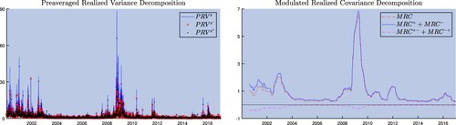
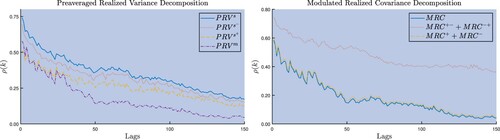
Figure 2 plots the autocorrelation function, averaged across all stocks for the PRV and MRC with their respective signed components. A cursory inspection shows a lower level of persistence when compared to standard volatility measures, which is expected since MMSN induces first-order autocorrelation (Hansen and Lunde 2006). The negative semi-variance shows higher persistence than its positive counterpart; thus being aligned with the findings of Patton and Sheppard (2015). Besides, the market is less persistent than the stocks. This may be in part explained by the memoryless large (finite) jumps typically observed in individual stocks (Duffie et al. 2000, Andersen et al. 2007, Duong and Swanson 2015, Bu et al. 2021), which however once aggregated at the market level become informative (Duong and Swanson 2015, Bu et al. 2021); thus reducing the persistence of $PR{V}^m$ compared to $PR{V}^s$. The MRC shows similar patterns as only the concordant elements are affected by co-jump activity (Bollerslev et al. 2020, Hizmeri et al. 2020).

Figure 2. Autocorrelation function.

The figure graphs the autocorrelation function for the different realized variances and covariances elements. The results presented are for the average across the stocks.

5. Modeling and forecasting with the market-HAR

5.1. In-sample performance

Table 3 presents the estimated coefficients and goodness-of-fit statistics for the HAR-PRV, HAR-V and HAR-Co-V models across three forecasting horizons: 1 day (h = 1), 1 week (h = 5), and 1 month (h = 22) ahead. The null hypothesis of the F-test is that of equal fit between the benchmark HAR-PRV and each of the market-HAR models; with the rejection indicating the latter outperforms the former. The number of stocks where the market-HAR models supersede the benchmark HAR-PRV is reported.

Table 3. Market-HAR prediction regression results.

	HAR-PRV	HAR-V	HAR-Co-V	HAR-PRV	HAR-V	HAR-Co-V	HAR-PRV	HAR-V	HAR-Co-V
	h = 1			h = 5			h = 22
${\text{β}}_0$	0.368${}^{\ast \ast \ast }$	0.355${}^{\ast \ast \ast }$	0.286${}^{\ast \ast \ast }$	0.502${}^{\ast \ast \ast }$	0.488${}^{\ast \ast \ast }$	0.412${}^{\ast \ast \ast }$	0.785${}^{\ast \ast \ast }$	0.752${}^{\ast \ast \ast }$	0.674${}^{\ast \ast \ast }$
${\text{β}}_d^s$	0.191${}^{\ast \ast \ast }$	0.158${}^{\ast \ast \ast }$	0.162${}^{\ast \ast \ast }$	0.117${}^{\ast \ast \ast }$	0.085${}^{\ast \ast }$	0.103	0.065	0.046	0.057
${\text{β}}_w^s$	0.335${}^{\ast \ast \ast }$	0.237${}^{\ast }$	0.259	0.291${}^{\ast \ast \ast }$	0.212${}^{\ast \ast \ast }$	0.196	0.200${}^{\ast \ast }$	0.137	0.199
${\text{β}}_m^s$	0.349${}^{\ast \ast \ast }$	0.406${}^{\ast \ast \ast }$	0.439${}^{\ast \ast \ast }$	0.421${}^{\ast \ast \ast }$	0.461${}^{\ast \ast \ast }$	0.524${}^{\ast \ast \ast }$	0.464${}^{\ast \ast \ast }$	0.501${}^{\ast \ast \ast }$	0.490${}^{\ast \ast \ast }$
${\text{β}}_d^m$		0.139	0.151		0.146${}^{\ast }$	0.242${}^{\ast }$		0.090	0.145
${\text{β}}_w^m$		0.406${}^{\ast \ast }$	0.395${}^{\ast }$		0.342${}^{\ast }$	0.045		0.180${}^{\ast }$	0.404
${\text{β}}_m^m$		−0.311	0.396		−0.257	0.773${}^{\ast }$		−0.081	0.648${}^{\ast }$
${\text{β}}_d^{MRC}$			−0.030			−0.128${}^{\ast }$			−0.077
${\text{β}}_w^{MRC}$			−0.067${}^{\ast }$			0.259			−0.353
${\text{β}}_m^{MRC}$			−0.729			−1.105			−0.718${}^{\ast }$
$R_{adj}^2$	0.389	0.398	0.403	0.551	0.566	0.575	0.564	0.583	0.598
F-test	–	20	20	–	18	20	–	20	20

Note: The table reports the coefficients for the average across all the stocks at the 300 seconds. ${}^{\ast }$, ${}^{\ast \ast }$, and ${}^{\ast \ast \ast }$ represent the significant of the coefficients at the 10%, 5%, and 1% levels using the Newey–West HAC correction allowing for serial correlation up to order 5 $(h=1)$, 10 (h = 5), and 44 (h = 22). Bold numbers highlight the market-HAR models that outperform the benchmark HAR-PRV. The bottom panel reports average values across all the stocks for the $R_{adj}^2$, and the number of rejections of the F-test. The F-test has a null hypothesis of equal fit, and hence its rejection indicates that market-HAR models are a better model fit than HAR-PRV models.

A first inspection of the results shows that adding market information in the HAR-V model leads to an improvement in the model fit relative to the benchmark model. This improvement ranges from 0.9% to 1.9% points in terms of the adjusted R-squares, and with the exception of two stocks at h = 5, the F-test rejects the null of equal fit for all the stocks across all forecasting horizons. Moreover, the HAR-Co-V model (which incorporates the variance and covariance market information) substantially improves the model fit: relative to the HAR-PRV models R-squares are raised from 1.4% to 3.4% points. The F-test corroborates this result. Market information renders stock-specific variables insignificant, which suggests that idiosyncratic volatility dynamics are of lesser importance. Monthly market volatility in the HAR-V model and the covariance estimates in the HAR-Co-V models are generally negative across all forecasting horizons. For the HAR-V model, negative market variance reduces weights assigned to monthly information; instead it places more emphasis on daily and weekly information.

Tables 4 and 5 present the parameter estimates and goodness-of-fit statistics for the asymmetric market-HAR variants. We discuss these tables in turn. Focusing first on the results in table 4, we observe that the specification based on the negative semi-variance has better fit than the one with the positive. Besides, the HAR-V${}^{-}$ outperforms the benchmark HAR-PRV in the majority of stocks. The increase in model fit is readily observed in terms of R-squares, where the HAR-V${}^{-}$ model improves between 3.4 % and 4.3% points relative to the HAR-PRV model, and between 1.5 % and 3.3% points relative to the unsigned HAR-V variant, across all forecasting horizons. Our findings here are in line with Patton and Sheppard (2015) who argue that negative semi-variances are more important to predict future volatility.

Table 4. Asymmetric HAR-V prediction regression results.

	HAR-V${}^{+}$	HAR-V${}^{-}$	HAR-V${}^{+}$	HAR-V${}^{-}$	HAR-V${}^{+}$	HAR-V${}^{-}$
	h = 1		h = 5		h = 22
${\text{β}}_0$	0.551${}^{\ast \ast \ast }$	0.326${}^{\ast \ast \ast }$	0.650${}^{\ast \ast \ast }$	0.480${}^{\ast \ast \ast }$	0.886${}^{\ast \ast \ast }$	0.757${}^{\ast \ast \ast }$
${\text{β}}_d^{s^{+}}$	0.149		0.083		0.041
${\text{β}}_w^{s^{+}}$	0.408		0.328		0.200
${\text{β}}_m^{s^{+}}$	0.888${}^{\ast \ast \ast }$		0.963${}^{\ast \ast \ast }$		1.004${}^{\ast \ast \ast }$
${\text{β}}_d^{m^{+}}$	−0.035		0.052		0.041
${\text{β}}_w^{m^{+}}$	0.780		0.663		0.414
${\text{β}}_m^{m^{+}}$	−0.276		−0.232		−0.026
${\text{β}}_d^{s^{-}}$		0.209${}^{\ast \ast \ast }$		0.112${}^{\ast }$		0.061
${\text{β}}_w^{s^{-}}$		0.429${}^{\ast }$		0.371${}^{\ast }$		0.263${}^{\ast }$
${\text{β}}_m^{s^{-}}$		0.884${}^{\ast \ast \ast }$		0.963${}^{\ast \ast \ast }$		0.980${}^{\ast \ast \ast }$
${\text{β}}_d^{m^{-}}$		0.995${}^{\ast \ast }$		0.627${}^{\ast \ast }$		0.357${}^{\ast }$
${\text{β}}_w^{m^{-}}$		0.857${}^{\ast }$		0.887${}^{\ast }$		0.407
${\text{β}}_m^{m^{-}}$		−0.897${}^{\ast }$		−0.652		−0.072
$R_{adj}^2$	0.335	0.431	0.497	0.594	0.526	0.598
F-test	0	19	1	20	1	20
HAR-PRV
$R_{adj}^2$	0.389		0.551		0.564

Note: See notes to table 3. The bottom panel of the table reports the 1-day (h = 1), 5-day (h = 5), and 22-day (h = 22) ahead HAR-PRV's adjusted R-squares for the average across all the stocks.

Table 5. Asymmetric HAR-Co-V prediction regression results.

Panel A: The table reports the prediction regression results for HAR-Co-V based on unsigned volatilities and semi-covariances.
	HAR-Co${}^{+}$-V	HAR-Co${}^{-}$-V	HAR-Co${}^{+}$-V	HAR-Co${}^{-}$-V	HAR-Co${}^{+}$-V	HAR-Co${}^{-}$-V
	h = 1		h = 5		h = 22
${\text{β}}_0$	0.160	0.311${}^{\ast \ast \ast }$	0.332${}^{\ast \ast }$	0.445${}^{\ast \ast \ast }$	0.614${}^{\ast \ast \ast }$	0.745${}^{\ast \ast \ast }$
${\text{β}}_d^s$	0.216${}^{\ast \ast }$	0.102	0.120${}^{\ast \ast \ast }$	0.051	0.063${}^{\ast \ast \ast }$	0.027
${\text{β}}_w^s$	0.326${}^{\ast \ast }$	0.121	0.281${}^{\ast \ast }$	0.114	0.194${}^{\ast \ast \ast }$	0.109
${\text{β}}_m^s$	0.417${}^{\ast \ast \ast }$	0.481${}^{\ast \ast \ast }$	0.489${}^{\ast \ast \ast }$	0.540${}^{\ast \ast \ast }$	0.551${}^{\ast \ast \ast }$	0.502${}^{\ast \ast \ast }$
${\text{β}}_d^m$	0.537${}^{\ast \ast }$	−0.149	0.377${}^{\ast \ast }$	−0.041	0.197${}^{\ast }$	−0.007
${\text{β}}_w^m$	0.859${}^{\ast }$	−0.278	0.692	−0.267	0.472	−0.059
${\text{β}}_m^m$	0.149	−0.081	0.295	0.145	0.643	−0.005
${\text{β}}_d^{R{C}^{+}}$	−0.727${}^{\ast \ast }$		−0.447${}^{\ast \ast }$		−0.232${}^{\ast }$
${\text{β}}_w^{R{C}^{+}}$	−1.159${}^{\ast }$		−0.882${}^{\ast }$		−0.751
${\text{β}}_m^{R{C}^{+}}$	−0.908		−1.103		−1.436${}^{\ast }$
${\text{β}}_d^{R{C}^{-}}$		0.896${}^{\ast \ast }$		0.532${}^{\ast \ast }$		0.309${}^{\ast }$
${\text{β}}_w^{R{C}^{-}}$		1.789${}^{\ast }$		1.617${}^{\ast }$		0.585
${\text{β}}_m^{R{C}^{-}}$		−0.719		−1.099		−0.237
$R_{adj}^2$	0.426	0.427	0.593	0.591	0.607	0.594
F-test	20	20	20	20	20	20
Panel B: The table reports the prediction regression results for HAR-Co-V using semi(co)variances.
	HAR-Co${}^{+}$-V${}^{+}$				HAR-Co${}^{-}$-V${}^{-}$
	h = 1	h = 5	h = 22		h = 1	h = 5	h = 22
${\text{β}}_0$	0.472${}^{\ast \ast \ast }$	0.583${}^{\ast \ast \ast }$	0.832${}^{\ast \ast \ast }$	${\text{β}}_0$	0.265${}^{\ast \ast }$	0.400${}^{\ast \ast \ast }$	0.698${}^{\ast \ast \ast }$
${\text{β}}_d^{s^{+}}$	0.238	0.155	0.085	${\text{β}}_d^{s^{-}}$	0.192${}^{\ast \ast \ast }$	0.123${}^{\ast \ast \ast }$	0.071
${\text{β}}_w^{s^{+}}$	0.570	0.435	0.316	${\text{β}}_w^{s^{-}}$	0.393${}^{\ast \ast \ast }$	0.293	0.394
${\text{β}}_m^{s^{+}}$	0.874${}^{\ast \ast }$	0.995${}^{\ast \ast }$	1.027${}^{\ast \ast }$	${\text{β}}_m^{s^{-}}$	1.067${}^{\ast \ast \ast }$	1.237${}^{\ast \ast \ast }$	1.056${}^{\ast \ast \ast }$
${\text{β}}_d^{m^{+}}$	0.273	0.337	0.202	${\text{β}}_d^{m^{-}}$	0.816	0.587${}^{\ast }$	0.367${}^{\ast }$
${\text{β}}_w^{m^{+}}$	1.478	1.007	0.831	${\text{β}}_w^{m^{-}}$	−0.005	−0.238	0.827
${\text{β}}_m^{m^{+}}$	0.684	0.938	1.085	${\text{β}}_m^{m^{-}}$	0.749${}^{\ast }$	1.755${}^{\ast }$	1.200
${\text{β}}_d^{MR{C}^{+}}$	−0.424	−0.377	−0.219	${\text{β}}_d^{MR{C}^{-}}$	0.122	0.004	−0.023
${\text{β}}_w^{MR{C}^{+}}$	−0.968	−0.541	−0.618	${\text{β}}_w^{MR{C}^{-}}$	0.772	1.026	−0.645
${\text{β}}_m^{MR{C}^{+}}$	−0.920	−1.200	−1.144	${\text{β}}_m^{MR{C}^{-}}$	−1.711${}^{\ast }$	−2.616${}^{\ast }$	−1.412${}^{\ast }$
$R_{adj}^2$	0.346	0.513	0.544	${\overline{R}}_{adj}^2$	0.436	0.603	0.609
F-test	0	3	4	F-test	19	20	20
HAR-PRV
$R_{adj}^2$	0.389	0.551	0.564

Note: See notes to table 3 for details. The bottom panel of the table reports the 1-day (h = 1), 5-day (h = 5), and 22-day (h = 22) ahead HAR-PRV's adjusted R-squares for the average across all the stocks.

In table 5, the asymmetric HAR-Co-V models are presented in two panels. Panel A gives parameter estimates for the HAR-Co-V models based on semi-covariances, but using unsigned volatilities. Across all forecasting horizons F-test values show both models to improve fit relative to the benchmark HAR-PRV model. The general similarity of goodness of fit across these models suggests similar explanatory power for the semi-covariances. Panel B reports the parameter estimates for the asymmetric HAR-Co-V using semi-covariances and semi-variances in the fully positive (HAR-Co${}^{+}$-V${}^{+}$) and negative (HAR-Co${}^{-}$-V${}^{-}$) variant. The HAR-Co${}^{-}$-V${}^{-}$ outperforms its fully positive counterpart by 6.5–9.0% points in terms of the adjusted R-squared, across all forecasting horizons. Compared to the benchmark HAR-PRV, the HAR-Co${}^{-}$-V${}^{-}$ model offers superior fit in most stocks.

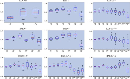
Figure 3 presents the distribution of model coefficients across the stocks using box-plots. The coefficient estimates appear well-behaved with the weekly and monthly components of the HAR-PRV model reflecting the stocks' heterogeneity to a greater extent than the daily component. This may be plausibly related to the mix of investor preferences observed at different stocks and/or business sectors. Across the models that contain both firm-specific and market-specific information, the marginal contribution of the latter varies substantially at the stock level, as evidenced by the higher heterogeneity of the market-specific coefficients vis-à-vis their firm-specific counterparts. A similar finding is observed for the models further allowing for realized covariances.¹⁸

Figure 3. Box plots for 1-day ahead parameter estimates.

Note: The figure depicts the box plot for each coefficient estimated across the nine different models. Each subplot shows the daily weekly and monthly coefficient pertaining to a specific model.

Our general findings are that, by incorporating market information, the market-HAR models deliver superior explanatory power over the benchmark HAR-PRV model. Whether the superior in-sample performance translates into out-of-sample forecasting gains is examined next.

5.2. Out-of-sample forecasting

Table 6 reports out-of-sample relative losses across forecasting horizons and sampling frequencies. Using each loss function, relative loss is computed as the ratio of the market-HAR models to the benchmark HAR-PRV model. For values below unity, market-HAR models outperform the benchmark. The superscript indicates stocks with significantly higher ($\alpha =0.05$ level) relative forecasting performance for market-HAR models, under the CPA test of Giacomini and White (2006). In line with the literature, we first discuss results based on the 300-second sampling frequency, 1-day ahead forecasting using the HMSE loss function.¹⁹ We then discuss in turn the impact of sampling frequency and longer forecasting horizon.

Table 6. Out-of-sample ranking performance.

	QLIKE	Rank	QLIKE	Rank	QLIKE	Rank	Avg.	HMSE	Rank	HMSE	Rank	HMSE	Rank	Avg.
	h = 1		h = 5		h = 22			h = 1		h = 5		h = 22
	30-second return							30-second return
HAR-PRV	1.000	6	1.000	7	1.000	7	1.000	1.000	7	1.000	7	1.000	7	1.000
HAR-V	0.980${}^{11}$	4	0.963${}^9$	6	0.976${}^3$	6	0.973	0.958${}^{13}$	6	0.955${}^9$	6	0.985${}^6$	6	0.966
HAR-V${}^{+}$	1.170${}^0$	9	1.154${}^0$	9	1.086${}^0$	9	1.137	1.363${}^0$	9	1.281${}^0$	9	1.160${}^1$	9	1.268
HAR-V${}^{-}$	0.939${}^{14}$	1	0.895${}^{17}$	1	0.937${}^6$	3	0.924	0.841${}^{19}$	3	0.868${}^{17}$	3	0.940${}^9$	5	0.883
HAR-Co-V	0.982${}^{11}$	5	0.958${}^9$	5	0.956${}^8$	5	0.965	0.922${}^{15}$	5	0.902${}^{13}$	5	0.912${}^{12}$	3	0.912
HAR-Co${}^{+}$-V${}^{+}$	1.149${}^1$	8	1.132${}^2$	8	1.059${}^4$	8	1.113	1.279${}^3$	8	1.206${}^5$	8	1.096${}^6$	8	1.194
HAR-Co${}^{-}$-V${}^{-}$	0.970${}^{10}$	3	0.900${}^{13}$	2	0.923${}^9$	2	0.931	0.835${}^{19}$	2	0.831${}^{18}$	2	0.885${}^{12}$	2	0.850
HAR-Co${}^{+}$-V	0.965${}^{10}$	2	0.905${}^{17}$	3	0.909${}^{11}$	1	0.926	0.791${}^{19}$	1	0.802${}^{19}$	1	0.848${}^{15}$	1	0.813
HAR-Co${}^{-}$-V	1.001${}^8$	7	0.928${}^9$	4	0.951${}^6$	4	0.960	0.887${}^{15}$	4	0.896${}^{11}$	4	0.936${}^9$	4	0.906
	60-second return							60-second return
HAR-PRV	1.000	6	1.000	7	1.000	7	1.000	1.000	7	1.000	7	1.000	7	1.000
HAR-V	0.976${}^{13}$	4	0.957${}^{10}$	6	0.972${}^6$	6	0.968	0.942${}^{15}$	6	0.939${}^{13}$	6	0.977${}^8$	6	0.953
HAR-V${}^{+}$	1.176${}^0$	9	1.168${}^0$	9	1.098${}^0$	9	1.147	1.377${}^0$	9	1.302${}^1$	9	1.179${}^0$	9	1.286
HAR-V${}^{-}$	0.945${}^{14}$	1	0.895${}^{16}$	1	0.935${}^6$	3	0.925	0.840${}^{17}$	3	0.866${}^{17}$	3	0.942${}^9$	5	0.883
HAR-Co-V	0.973${}^{15}$	3	0.949${}^{10}$	5	0.952${}^9$	5	0.958	0.899${}^{16}$	5	0.881${}^{15}$	5	0.902${}^{12}$	3	0.894
HAR-Co${}^{+}$-V${}^{+}$	1.147${}^1$	8	1.133${}^4$	8	1.061${}^3$	8	1.114	1.263${}^3$	8	1.201${}^4$	8	1.095${}^3$	8	1.186
HAR-Co${}^{-}$-V${}^{-}$	0.964${}^{13}$	2	0.901${}^{13}$	3	0.921${}^7$	2	0.929	0.820${}^{19}$	2	0.822${}^{19}$	2	0.881${}^{12}$	2	0.841
HAR-Co${}^{+}$-V	0.984${}^9$	5	0.897${}^{17}$	2	0.902${}^{12}$	1	0.927	0.763${}^{20}$	1	0.779${}^{20}$	1	0.833${}^{15}$	1	0.792
HAR-Co${}^{-}$-V	1.024${}^7$	7	0.924${}^{10}$	4	0.944${}^8$	4	0.964	0.869${}^{15}$	4	0.876${}^{13}$	4	0.921${}^{10}$	4	0.889
	300-second return							300-second return
HAR-PRV	1.000	7	1.000	7	1.000	7	1.000	1.000	7	1.000	7	1.000	7	1.000
HAR-V	0.966${}^{16}$	3	0.943${}^{16}$	6	0.963${}^8$	6	0.957	0.902${}^{15}$	6	0.909${}^{14}$	6	0.961${}^{10}$	6	0.924
HAR-V${}^{+}$	1.174${}^0$	9	1.198${}^2$	9	1.138${}^1$	9	1.170	1.408${}^0$	9	1.384${}^2$	9	1.260${}^1$	9	1.350
HAR-V${}^{-}$	0.963${}^{14}$	2	0.901${}^{15}$	2	0.930${}^{10}$	3	0.931	0.818${}^{17}$	3	0.855${}^{15}$	4	0.939${}^{12}$	5	0.871
HAR-Co-V	0.959${}^{16}$	1	0.923${}^{16}$	4	0.936${}^8$	4	0.940	0.823${}^{15}$	4	0.817${}^{17}$	3	0.857${}^{14}$	3	0.833
HAR-Co${}^{+}$-V${}^{+}$	1.135${}^2$	8	1.142${}^4$	8	1.085${}^4$	8	1.121	1.249${}^4$	8	1.220${}^4$	8	1.138${}^3$	8	1.202
HAR-Co${}^{-}$-V${}^{-}$	0.983${}^{12}$	4	0.911${}^{14}$	3	0.909${}^{12}$	2	0.934	0.765${}^{17}$	2	0.781${}^{18}$	2	0.842${}^{15}$	2	0.796
HAR-Co${}^{+}$-V	0.985${}^{12}$	5	0.881${}^{19}$	1	0.885${}^{14}$	1	0.917	0.693${}^{19}$	1	0.729${}^{20}$	1	0.806${}^{16}$	1	0.743
HAR-Co${}^{-}$-V	0.995${}^8$	6	0.931${}^{12}$	5	0.944${}^8$	5	0.957	0.868${}^{15}$	5	0.880${}^{1}4$	5	0.931${}^{12}$	4	0.893

Note: The table reports the average relative loss for QLIKE and HMSE across all the stocks. The relative losses are estimated as the ratio of the losses of the market-HAR models to the losses of the benchmark HAR-PRV. Entries in bold indicate that our proposed models outperform the HAR-PRV. Avg. column reports for each model the average relative loss across all forecasting horizons. The number in the superscript represents the number of stocks for which the losses of the market-HAR models are significantly lower than the losses of the benchmark model. We use the CPA test of Giacomini and White (2006) at the 5% significance level.

A first inspection of the results shows the most parsimonious of the market-HAR models (i.e. the HAR-V) to outperform the benchmark HAR-PRV model by approximately 9.80% points, and 15 stocks display significant forecasting gains. Asymmetric market-HAR models provide even better out-of-sample forecasting performance: when the negative semi-variance is used, the HAR-V${}^{-}$ model is relatively superior by 18.20% points, and 17 stocks display significant forecasting gains. Market-HAR models that incorporate realized covariance information outperform by up to 30.70% points the benchmark HAR-PRV model, with significant results for most stocks.

The forecasting gains of market-HAR models are moderated at high sampling frequencies and longer forecasting horizons.²⁰ Nevertheless, these remain highly significant even at the 30-second sampling frequency and/or the 1-month ahead case. In particular, the HAR-Co${}^{+}$-V model outperforms the benchmark by 20.9% points with significant results in 19 stocks when the sampling frequency is set at the 30-second, and by 19.40% points when the forecasting horizon is set to 1-month ahead.

5.3. Model classification and performance

This section presents the results of the Model Confidence Set (MCS) approach, which identifies the subset of models from the many market-HAR specifications with a superior predictive ability across specific forecasting horizons and sampling frequencies. The small variation in the ranking of models, as attributed to noise-robust realized measures, gives confirmation that, after accounting for MMSN, the sampling frequency choice becomes insignificant.

Table 7 reports MCS ranking information for individual stocks across forecasting horizons when the 300-second sampling frequency is used for the realized measures. Retained models are identified by a ranking number; models excluded from the MCS are identified by a dash. Models ranked higher outperform those ranked lower. The MCS results reported are based on the QLIKE loss function.²¹ Focusing on the 1-day ahead results, we observe that for most stocks (i.e. 18/20) there are at least two competing models in the MCS, while only 3/20 stocks include the HAR-PRV model—the main benchmark in the previous part of the analysis. The last two columns show respectively the percentage of times a model has been included in the MCS and its average rank. The HAR-V${}^{-}$ and HAR-Co${}^{+}$-V models are predominantly selected by the MCS featuring in 70% of the stocks; while the former has an average ranking of 2.86, the latter ranks at 1.86. Therefore the MCS finds the HAR-Co${}^{+}$-V the best model, on average. The 1-month forecasts show that the HAR-Co${}^{+}$-V model expands to 90% of the stocks, with its average ranking dropping to 1.44; thus further dominating the other models.

Table 7. Model confidence set ranking across forecasting horizons.

	AMZN	ARCN	BA	BAC	CAT	CHL	COST	CSCO	DIS	DOW	EXC	FCX	HAL	HON	IBM	KO	PG	SO	WFC	XRX	N%	Rank
	h = 1
HAR-PRV	–	4	–	–	7	–	–	–	–	–	2	–	–	–	–	–	–	–	–	–	15	4.33
HAR-V	–	2	–	–	6	–	–	–	–	–	1	–	4	–	–	2	4	1	5	–	40	3.13
HAR-V${}^{+}$	–	–	–	–	–	–	–	–	–	–	–	–	–	–	–	–	–	–	–	–	0	–
HAR-V${}^{-}$	1	6	–	–	4	3	1	2	–	2	–	–	3	3	3	5	3	3	1	–	70	2.86
HAR-Co-V	3	3	2	3	3	4	–	–	2	–	–	1	2	–	–	1	1	2	–	2	65	2.23
HAR-Co${}^{+}$-V${}^{+}$	–	–	–	–	–	–	–	–	–	–	–	–	–	–	–	–	–	–	–	–	0	–
HAR-Co${}^{-}$-V${}^{-}$	–	–	–	4	2	1	–	1	4	3	–	–	5	4	1	3	2	–	2	–	60	2.67
HAR-Co${}^{+}$-V	2	5	1	1	1	2	–	–	1	1	–	–	1	1	2	–	–	4	3	1	70	1.86
HAR-Co${}^{-}$-V	–	1	3	2	5	–	–	–	3	–	–	–	–	2	–	4	–	–	4	–	40	3.00
	h = 5
HAR-PRV	–	–	–	–	–	–	–	–	–	–	3	–	–	–	–	–	–	–	–	–	5	3.00
HAR-V	–	–	–	–	–	–	–	–	–	–	1	4	–	–	–	6	–	–	–	–	15	3.67
HAR-V${}^{+}$	–	–	–	–	–	–	–	–	–	–	–	–	–	–	–	–	–	–	–	–	0	–
HAR-V${}^{-}$	–	3	–	2	3	–	1	1	–	3	2	6	–	3	3	3	4	3	2	–	70	2.79
HAR-Co-V	–	4	2	–	–	–	–	–	2	–	4	1	2	–	–	2	2	2	4	2	55	2.45
HAR-Co${}^{+}$-V${}^{+}$	–	–	–	–	–	–	–	–	–	–	–	–	–	–	–	–	–	–	–	–	0	–
HAR-Co${}^{-}$-V${}^{-}$	–	–	4	3	1	2	2	2	–	1	–	5	–	4	1	1	1	–	3	–	65	2.31
HAR-Co${}^{+}$-V	1	1	1	1	2	1	–	–	1	2	–	3	1	1	2	4	3	1	1	1	85	1.59
HAR-Co${}^{-}$-V	–	2	3	4	–	–	–	–	–	–	–	2	–	2	–	5	–	–	–	3	35	3.00
	h = 22
HAR-PRV	2	3	–	6	4	–	–	–	–	–	–	7	–	–	2	–	–	–	–	–	30	4.00
HAR-V	–	4	–	3	–	–	–	–	–	–	–	5	–	–	–	–	–	–	–	–	15	4.00
HAR-V${}^{+}$	–	–	–	–	–	–	–	–	–	–	–	–	–	–	–	–	–	–	–	–	0	–
HAR-V${}^{-}$	–	2	–	4	3	2	1	1	–	3	2	6	–	2	–	4	–	–	2	5	65	2.85
HAR-Co-V	3	6	–	5	5	–	–	–	2	4	–	4	1	–	–	5	2	–	–	4	55	3.45
HAR-Co${}^{+}$-V${}^{+}$	–	–	–	–	–	–	–	–	4	–	–	–	–	–	–	–	–	–	–	–	5	4.00
HAR-Co${}^{-}$-V${}^{-}$	–	5	–	2	1	3	2	–	3	1	3	3	–	–	1	1	1	–	–	3	65	2.23
HAR-Co${}^{+}$-V	1	1	1	1	2	1	–	–	1	2	1	1	2	1	3	2	3	1	1	1	90	1.44
HAR-Co${}^{-}$-V	–	7	–	7	6	–	3	–	–	–	–	2	3	–	4	3	–	–	–	2	40	3.75

Note: The table reports the ranking based on the Model Confidence Set (MCS) proposed by Hansen et al. (2011). The entries are the ranking of the models across each stock and forecasting horizon based on noise-robust measures estimated using 300-second return frequency. We use the QLIKE as loss function, and the MCS is estimated using a block bootstrap with a window equal to 10 days, 5000 replications, and a significance level of 10%. The dash-line indicates that the model has been excluded from the MCS. The N% and Rank columns show the percentage of times a model has been included in the MCS and its average rank respectively.

Table 8 gives MCS rankings for individual stocks across sampling frequencies at the 1-day ahead forecasting horizon. The MCS results obtained with the 150-second sampling frequency show that HAR-Co${}^{+}$-V is the best model for 70% of the stocks with an average ranking of 1.64; thus being comparable to the results reported in table 7. However, as the sampling frequency increases the HAR-V${}^{-}$ emerges as the best specification in 80–90.0% of the stocks. It appears that the negative semi-variance dominates at higher frequencies, while the positive one carries no predictive power. In broad strokes, these asymmetric models show superior forecasting performance, which is in line with the findings of Patton and Sheppard (2015) and Bollerslev et al. (2016) among others. The new information that our paper uncovers relates to which signed components contribute to the most significant gains in the presence of both stock-specific and market-specific signed realized measures as well as their signed realized covariances. It further reveals that despite negative semi-variances being regarded as more informative, there is merit in the information content afforded by the positive semi-covariance.

Table 8. Model confidence set across sampling frequencies.

	AMZN	ARCN	BA	BAC	CAT	CHL	COST	CSCO	DIS	DOW	EXC	FCX	HAL	HON	IBM	KO	PG	SO	WFC	XRX	N%	Rank
	30-second return
HAR-PRV	–	1	–	–	4	–	–	–	–	–	–	–	–	–	–	–	–	–	–	–	10	2.50
HAR-V	–	2	–	–	5	–	–	–	–	–	–	2	–	–	–	2	–	–	–	3	25	2.80
HAR-V${}^{+}$	–	–	–	–	–	–	–	–	–	–	–	–	–	–	–	–	–	–	–	–	0	–
HAR-V${}^{-}$	1	3	–	1	1	2	1	1	3	1	–	1	5	1	2	1	2	2	1	2	90	1.72
HAR-Co-V	2	4	3	–	3	–	–	–	–	–	1	3	3	–	–	3	4	–	–	6	50	3.20
HAR-Co${}^{+}$-V${}^{+}$	–	–	–	–	–	–	–	–	–	–	–	–	–	–	–	–	–	–	–	–	0	–
HAR-Co${}^{-}$-V${}^{-}$	–	7	–	4	–	3	2	2	2	4	–	4	4	2	–	–	3	–	–	4	60	3.42
HAR-Co${}^{+}$-V	3	6	1	3	2	1	3	–	1	2	–	–	1	–	1	4	1	1	–	5	75	2.33
HAR-Co${}^{-}$-V	–	5	2	2	–	–	–	–	–	3	–	–	2	3	–	–	–	–	–	1	35	2.57
	60-second return
HAR-PRV	–	2	4	–	5	–	–	–	–	–	–	–	–	–	–	–	–	–	–	–	15	3.67
HAR-V	–	1	–	–	–	5	–	–	–	–	–	3	–	–	–	3	–	4	–	3	30	3.17
HAR-V${}^{+}$	–	–	–	–	–	–	–	–	–	–	–	–	–	–	–	–	–	–	–	–	0	–
HAR-V${}^{-}$	1	5	–	3	2	1	1	1	–	1	–	2	5	3	2	1	1	3	1	–	80	2.06
HAR-Co-V	3	3	2	–	3	4	–	–	–	–	1	1	3	–	–	2	4	2	–	2	60	2.50
HAR-Co${}^{+}$-V${}^{+}$	–	–	–	–	–	–	–	–	–	–	–	–	–	–	–	–	–	–	–	–	0	–
HAR-Co${}^{-}$-V${}^{-}$	–	–	–	4	4	3	2	2	–	4	–	5	4	2	3	4	2	–	–	–	60	3.25
HAR-Co${}^{+}$-V	2	–	1	1	1	2	3	–	1	2	–	4	1	4	1	–	3	1	–	–	70	1.93
HAR-Co${}^{-}$-V	–	4	3	2	–	–	–	–	–	3	–	–	2	1	–	–	–	–	–	1	35	2.29
	150-second return
HAR-PRV	–	4	4	–	–	–	–	–	–	–	3	–	–	–	–	–	–	–	–	–	15	3.67
HAR-V	–	2	–	–	–	–	–	–	–	–	1	–	–	–	–	2	4	2	–	–	25	2.20
HAR-V${}^{+}$	–	–	–	–	–	–	–	–	–	–	–	–	–	–	–	–	–	–	–	–	0	–
HAR-V${}^{-}$	1	6	–	–	4	2	1	1	–	2	–	–	–	–	–	4	3	4	1	–	55	2.64
HAR-Co-V	2	5	2	–	3	3	–	–	–	–	2	1	2	–	–	1	2	3	–	2	60	2.33
HAR-Co${}^{+}$-V${}^{+}$	–	–	–	–	–	–	–	–	–	–	–	–	–	–	–	–	–	–	–	–	0	–
HAR-Co${}^{-}$-V${}^{-}$	–	–	–	3	2	1	–	2	–	3	–	–	4	3	1	3	1	–	3	–	55	2.36
HAR-Co${}^{+}$-V	–	3	1	1	1	4	2	–	1	1	–	–	1	2	2	–	–	1	2	1	70	1.64
HAR-Co${}^{+}$-V	–	1	3	2	–	–	–	–	–	4	–	–	3	1	–	5	5	–	–	–	40	3.00

Note: The table reports the ranking based on the Model Confidence Set (MCS) proposed by Hansen et al. (2011). The entries are the ranking of the models across sampling frequencies based on 1-day ahead pseudo out-of-sample forecasts. We use the QLIKE as loss function, and the MCS is estimated using a block bootstrap with a window equal to 10 days, 5000 replications, and a significance level of 10%. The dash-line indicates that the model has been excluded from the MCS. The N% and Rank columns show the percentage of times a model has been included in the MCS and its average rank respectively.

5.4. Mixed sampling frequency market-HAR

In this section, we gauge the forecasting performance of the market-HAR models when we individually vary the sampling frequency on the stock and the market. Our earlier results have shown that the market-HAR models generally outperform the benchmark HAR-PRV and that the forecasting gains are of comparable magnitude across sampling frequencies. However, the results in table 2 reveal different correlation levels across sampling frequencies. Besides, the use noise-robust realized measures enable us to use a wide span of sampling frequencies.

We setup the mixed sampling approach on the HAR-V model for two reasons. First, the HAR-V model is the most parsimonious of the market-HAR class of models, hence our results here would be useful to establish a minimum expected gain. Second, the HAR-Co-V model incorporates the realized covariation that has to be estimated at the same sampling frequency between the stock and the market.²² The mixed-sampling HAR-V model is constructed by holding constant the stock frequency, while varying the market frequency and vice versa. We use a total of six sampling frequencies ranging from 30 to 300 seconds. The results are compared against the benchmark HAR-PRV and the HAR-V models that are based on the same sampling frequency for the stock and the market.

The results of this exercise are presented in table 9. The forecast evaluation criteria, averaged across all stocks, are presented in Panel A, while the relative losses with respect to the same frequency case (main diagonal) are reported in panel B. Figure 4 plots the relative losses in a 3D plane. The x- and y-axes display respectively the sampling frequency of the market and the stock, while the z-axis displays the loss ratio for the QLIKE (left-panel) and HMSE (right-panel). The darker part of the figure highlights the best performance, while by contrast the lighter part indicates the worst performance.

Figure 4. Mixed sampling HAR-V model.

Note: The figure depicts the out-of-sample average relative loss for a mixed sampling HAR-V model. The model is estimated by varying the sampling frequency used to estimate the stock and index volatility. The left-panel plots the QLIKE loss ratio surface, and the right-panel plots the HMSE loss ratio surface.

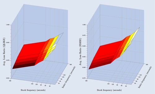
Table 9. Mixed sampling market-HAR.

	Panel A: Forecast evaluation criteria
	Index frequency
Stock frequency	30-sec	60-sec	90-sec	120-sec	150-sec	300-sec	30-sec	60-sec	90-sec	120-sec	150-sec	300-sec
	QLIKE						HMSE
30-sec	0.9801	0.9799	0.9792	0.9801	0.9806	0.9805	0.9577	0.9562	0.9549	0.9566	0.9569	0.9584
60-sec	0.9760	0.9764	0.9763	0.9771	0.9778	0.9782	0.9423	0.9421	0.9420	0.9434	0.9445	0.9469
90-sec	0.9719	0.9726	0.9729	0.9737	0.9745	0.9754	0.9303	0.9311	0.9319	0.9334	0.9347	0.9375
120-sec	0.9696	0.9705	0.9710	0.9717	0.9726	0.9740	0.9232	0.9243	0.9253	0.9267	0.9283	0.9319
150-sec	0.9666	0.9676	0.9681	0.9689	0.9697	0.9712	0.9123	0.9137	0.9151	0.9166	0.9182	0.9221
300-sec	0.9613	0.9622	0.9627	0.9634	0.9642	0.9659	0.8913	0.8933	0.8950	0.8968	0.8983	0.9021
	Panel B: Relative losses
	Index frequency
Stock frequency	30-sec	60-sec	90-sec	120-sec	150-sec	300-sec	30-sec	60-sec	90-sec	120-sec	150-sec	300-sec
	QLIKE						HMSE
30-sec	1.000	1.004	1.006	1.009	1.011	1.015	1.000	1.015	1.025	1.032	1.042	1.062
60-sec	0.996	1.000	1.003	1.006	1.008	1.013	0.984	1.000	1.011	1.018	1.029	1.050
90-sec	0.992	0.996	1.000	1.002	1.005	1.010	0.971	0.988	1.000	1.007	1.018	1.039
120-sec	0.989	0.994	0.998	1.000	1.003	1.008	0.964	0.981	0.993	1.000	1.011	1.033
150-sec	0.986	0.991	0.995	0.997	1.000	1.005	0.953	0.970	0.982	0.989	1.000	1.022
300-sec	0.981	0.985	0.990	0.991	0.994	1.000	0.931	0.948	0.960	0.968	0.978	1.000

Note: The table reports the mixed sampling market-HAR results. Panel A reports the forecasting evaluation criteria; Panel B reports the relative loss that is computed as the ratio of mixed sampling market-HAR models relative to the same frequency one (main diagonal). In panel A, values below unity indicate that the mixed sampling market-HAR outperforms the benchmark HAR-PRV. In panel B, values below unity indicate that the mixed frequency market-HAR models outperform the same frequency ones.

Interesting observations can be drawn from these results. First, all the sampling frequency combinations outperform the benchmark HAR-PRV model, thus corroborating our previous findings on the benefits of incorporating market information upon volatility forecasting. Second, the relative losses reported in the lower (upper) triangular part of each panel are below (above) unity suggesting that using a mixed sampling frequency market-HAR affects the forecasting performance. We observe that the best forecasting performance is achieved when the market sampling frequency is higher than the stock's. In particular and using the QLIKE (HMSE), the mixed sampling market-HAR shows 1.90% (6.90%) points superior forecasting performance when the 300-second stock sampling frequency is combined with the 30-second market sampling frequency. Forecasting improves proportionally to the differential in sampling frequencies between the stock and the market, while for those cases where stock sampling frequency is lower than the market, forecasting deteriorates. This observation suggests that the use of a mixed-sampling approach better captures variations in the information set of the stock and the market.

5.5. Economic value analysis

Table 10 reports the economic gains of switching from the benchmark HAR-PRV strategy to the market-HAR class of models for the 1-day ahead case.²³ The performance fee represents the amount that an investor is willing to pay to using our new class of forecasting models, and the performance fee is expressed in annual basis points. Statistically significant differentials are evaluated against the null hypothesis of zero performance fee using a one-sided t-test with a robust variance–covariance estimator following Engle and Colacito (2006), Bandi et al. (2008), and Nolte and Xu (2015), namely: $H_0:{\mathrm{\Delta }}_{\gamma }=0$ and $H_1:{\mathrm{\Delta }}_{\gamma }>0$. Bold numbers highlight the market-HAR models that outperform the benchmark strategy, and starred values indicate significant gains at the 5% significance level.

Table 10. Volatility-timing portfolio performance fee.

	AMZN	ARNC	BA	BAC	CAT	CHL	COST	CSCO	DIS	DOW	EXC	FCX	HAL	HON	IBM	KO	PG	SO	WFC	XRX	${\overline{\mathrm{\Delta }}}_{\gamma }$
	$\gamma =2$
HAR-V	2.428${}^{\star }$	–	−0.190	3.822${}^{\star }$	−0.123	0.053	4.152${}^{\star }$	0.192	−1.909	1.069	1.530	0.138	0.246	−0.360	1.366	0.025	4.878${}^{\star }$	0.200	0.045	45.464${}^{\star }$	3.151
HAR-V${}^{+}$	−22.394	–	−1.356	−4.885	−1.226	−1.211	−10.435	−2.541	−5.006	−3.453	0.703	0.051	−0.028	−2.990	−37.601	−5.667	−1.377	−0.569	−1.018	8.553${}^{\star }$	−4.622
HAR-V${}^{-}$	23.481${}^{\star }$	–	−0.116	12.288${}^{\star }$	0.330	1.358	20.431${}^{\star }$	5.117${}^{\star }$	−2.118	3.329${}^{\star }$	3.418${}^{\star }$	−0.020	0.413	0.688	29.539${}^{\star }$	4.330${}^{\star }$	7.985${}^{\star }$	1.017	0.893	49.685${}^{\star }$	8.102
HAR-Co-V	10.060${}^{\star }$	–	0.132	10.004${}^{\star }$	0.112	0.333	4.343${}^{\star }$	1.413	6.891${}^{\star }$	3.034${}^{\star }$	2.565${}^{\star }$	0.234	0.386	−0.477	14.087${}^{\star }$	2.384${}^{\star }$	19.123${}^{\star }$	1.213	0.648	50.339${}^{\star }$	6.341
HAR-Co${}^{+}$-V${}^{+}$	−8.855	–	−0.666	−1.433	−1.024	−0.973	−11.203	−2.404	4.982${}^{\star }$	−2.110	2.044${}^{\star }$	0.128	0.203	−1.716	−28.601	−3.457	8.035${}^{\star }$	0.718	−0.761	13.699${}^{\star }$	−1.670
HAR-Co${}^{-}$-V${}^{-}$	27.332${}^{\star }$	–	0.044	16.833${}^{\star }$	1.099	1.750	30.348${}^{\star }$	5.467${}^{\star }$	3.548${}^{\star }$	6.911${}^{\star }$	3.482${}^{\star }$	0.010	0.299	0.704	40.720${}^{\star }$	10.123${}^{\star }$	16.826${}^{\star }$	1.292	0.904	49.144${}^{\star }$	10.842
HAR-Co${}^{+}$-V	46.439${}^{\star }$	–	0.846	12.778${}^{\star }$	0.412	3.157${}^{\star }$	8.474${}^{\star }$	9.682${}^{\star }$	12.136${}^{\star }$	4.258${}^{\star }$	4.125${}^{\star }$	0.221	0.622	2.614${}^{\star }$	31.659${}^{\star }$	7.670${}^{\star }$	30.873${}^{\star }$	2.092${}^{\star }$	3.546${}^{\star }$	57.437${}^{\star }$	11.952
HAR-Co${}^{-}$-V	46.039${}^{\star }$	–	0.320	10.732${}^{\star }$	−0.001	−0.369	35.017${}^{\star }$	3.799${}^{\star }$	0.525	1.527	1.886	0.196	0.242	2.277${}^{\star }$	14.745${}^{\star }$	0.794	2.783${}^{\star }$	0.444	0.192	44.705${}^{\star }$	8.293
	$\gamma =6$
HAR-V	0.809	–	−0.063	1.274	−0.041	0.018	1.384	0.064	−0.636	0.356	0.510	0.046	0.082	−0.120	0.455	0.008	1.626	0.067	0.015	15.155${}^{\star }$	1.050
HAR-V${}^{+}$	−7.465	–	−0.452	−1.628	−0.409	−0.404	−3.478	−0.847	−1.669	−1.151	0.234	0.017	−0.009	−0.997	-12.534	−1.889	−0.459	−0.190	−0.339	2.851${}^{\star }$	−1.541
HAR-V${}^{-}$	7.827${}^{\star }$	–	−0.039	4.096${}^{\star }$	0.110	0.453	6.810${}^{\star }$	1.706	−0.706	1.110	1.139	−0.007	0.138	0.229	9.846${}^{\star }$	1.443	2.662${}^{\star }$	0.339	0.298	16.562${}^{\star }$	2.701
HAR-Co-V	3.353${}^{\star }$	–	0.044	3.335${}^{\star }$	0.037	0.111	1.448	0.471	2.297${}^{\star }$	1.011	0.855	0.078	0.129	−0.159	4.696${}^{\star }$	0.795	6.374${}^{\star }$	0.404	0.216	16.780${}^{\star }$	2.114
HAR-Co${}^{+}$-V${}^{+}$	−2.952	–	−0.222	−0.478	−0.341	−0.324	−3.734	−0.801	1.661	−0.703	0.681	0.043	0.068	−0.572	−9.534	−1.152	2.678${}^{\star }$	0.239	−0.254	4.566${}^{\star }$	−0.557
HAR-Co${}^{-}$-V${}^{-}$	9.111${}^{\star }$	–	0.015	5.611${}^{\star }$	0.366	0.583	10.234${}^{\star }$	1.822	1.183	2.304${}^{\star }$	1.161	0.003	0.100	0.235	13.573${}^{\star }$	3.374${}^{\star }$	5.609${}^{\star }$	0.431	0.301	16.381${}^{\star }$	3.620
HAR-Co${}^{+}$-V	15.587${}^{\star }$	–	0.282	4.259${}^{\star }$	0.137	1.052	2.825${}^{\star }$	3.233${}^{\star }$	4.045${}^{\star }$	1.419	1.375	0.074	0.207	0.871	10.553${}^{\star }$	2.557${}^{\star }$	10.515${}^{\star }$	0.697	1.185	19.146${}^{\star }$	4.001
HAR-Co${}^{-}$-V	15.914${}^{\star }$	–	0.107	3.577${}^{\star }$	−0.000	−0.123	11.672${}^{\star }$	1.266	0.175	0.509	0.629	0.065	0.081	0.759	4.915${}^{\star }$	0.265	0.928	0.148	0.064	14.902${}^{\star }$	2.793
	$\gamma =10$
HAR-V	0.486	–	−0.038	0.764	−0.025	0.011	0.830	0.038	−0.382	0.214	0.306	0.028	0.049	−0.072	0.273	0.005	0.976	0.040	0.009	9.093${}^{\star }$	0.630
HAR-V${}^{+}$	−4.479	–	−0.271	−0.977	−0.245	−0.242	−2.087	−0.508	−1.001	−0.691	0.141	0.010	−0.006	−0.598	−7.520	−1.133	−0.275	−0.114	−0.204	1.711	−0.924
HAR-V${}^{-}$	4.696${}^{\star }$	–	−0.023	2.458${}^{\star }$	0.066	0.272	4.086${}^{\star }$	1.023	−0.424	0.666	0.684	−0.004	0.083	0.138	5.908${}^{\star }$	0.866	1.597	0.203	0.179	9.937${}^{\star }$	1.620
HAR-Co-V	2.012${}^{\star }$	–	0.026	2.001	0.022	0.067	0.869	0.283	1.378	0.607	0.513	0.047	0.077	−0.095	2.817${}^{\star }$	0.477	3.825${}^{\star }$	0.243	0.130	10.068${}^{\star }$	1.268
HAR-Co${}^{+}$-V${}^{+}$	−1.771	–	−0.133	−0.287	−0.205	−0.195	−2.241	−0.481	0.996	−0.422	0.409	0.026	0.041	−0.343	−5.720	−0.691	1.607	0.144	−0.152	2.740${}^{\star }$	−0.334
HAR-Co${}^{-}$-V${}^{-}$	5.466${}^{\star }$	–	0.009	3.367${}^{\star }$	0.220	0.350	6.141${}^{\star }$	1.093	0.710	1.382	0.696	0.002	0.060	0.141	8.144${}^{\star }$	2.025${}^{\star }$	3.365${}^{\star }$	0.258	0.181	9.829${}^{\star }$	2.172
HAR-Co${}^{+}$-V	9.352${}^{\star }$	–	0.169	2.556${}^{\star }$	0.082	0.631	1.695	1.940${}^{\star }$	2.427${}^{\star }$	0.852	0.825	0.044	0.124	0.523	6.332${}^{\star }$	1.534	6.342${}^{\star }$	0.418	0.711	11.487${}^{\star }$	2.402
HAR-Co${}^{-}$-V	9.549${}^{\star }$	–	0.064	2.146${}^{\star }$	−0.000	−0.074	7.003${}^{\star }$	0.760	0.105	0.305	0.377	0.039	0.048	0.455	2.949${}^{\star }$	0.159	0.557	0.089	0.038	8.941${}^{\star }$	1.676

Note: The table shows results for the volatility-timing portfolio strategy using 1-day ahead forecasts. We report the economic gains of switching from the HAR-PRV model to the market-HAR models in annual basis points ${\mathrm{\Delta }}_{ab}$. The last column, ${\overline{\mathrm{\Delta }}}_{\gamma }$, reports the average performance fee for each model across all the stocks under analysis. Bold numbers highlight the market-HAR strategies that outperform the benchmark HAR-PRV strategy, and the starred values indicate that our strategy is significantly better than the benchmark in terms of performance fee evaluated at the 5% significance level. The empty columns for ARNC are because its expected return is always negative. Since short selling is not allowed and negative returns produce negative weights, an investor in this scenario can only select the risk-free rate.

A cursory inspection of the results finds that market-HAR models generate positive performance fees across all stocks. The best performance is achieved by the HAR-V${}^{-}$, HAR-Co${}^{+}$-V, and HAR-Co${}^{-}$-V${}^{-}$ strategies. When $\gamma =2$, these significantly outperform the benchmark strategy in at least 50% of our stocks. In contrast, the HAR-V${}^{+}$ and HAR-Co${}^{+}$-V${}^{+}$ models, that are based on the uninformative positive semi-variance, deliver weak out-of-sample performance. Performance fees at higher levels of risk aversion ($\gamma =6,10$) are positive and comparable to the $\gamma =2$ case.

To be allowed to switch from the benchmark strategy to the HAR-Co${}^{+}$-V strategy, a hypothetical investor would be willing to pay between 57 ($\gamma =2$) and 11 ($\gamma =10$) basis points. Regardless of the performance of HAR-V${}^{+}$ or HAR-Co${}^{+}$-V${}^{+}$, if HAR-V strategies were positioned at $\gamma =2$, a fee of 5.627 basis points would be warranted. Alternatively, HAR-Co-V strategies would, on average, warrant a performance fee of 9.357 basis points. These illustrative values highlight the benefits of incorporating market information in stock volatility forecasting; and that utilizing covariance and/or signed realized measures would further enhance the performance.

Table 11 presents the performance fee, averaged across all stocks for 1-day ahead forecasts when transaction costs are considered. These values are slightly smaller than earlier results, so indicating that transaction costs have only marginal impact upon strategies. The superior performance of the market-HAR models is not challenged by realistic transaction costs.

Table 11. Volatility-timing portfolio performance fee with transaction costs.

	${\overline{\mathrm{\Delta }}}_2$	TO	${\overline{\mathrm{\Delta }}}_6$	TO	${\overline{\mathrm{\Delta }}}_{10}$	TO
HAR-PRV		0.0041		0.0014		0.0008
HAR-V	3.135	0.0047	1.045	0.0016	0.627	0.0009
HAR-V${}^{+}$	−4.595	0.0031	−1.532	0.0010	−0.919	0.0006
HAR-V${}^{-}$	7.985	0.0083	2.663	0.0028	1.598	0.0017
HAR-Co-V	6.300	0.0056	2.101	0.0019	1.260	0.0011
HAR-Co${}^{+}$-V${}^{+}$	−1.661	0.0038	−0.554	0.0013	−0.332	0.0008
HAR-Co${}^{-}$-V${}^{-}$	10.691	0.0095	3.571	0.0032	2.143	0.0019
HAR-Co${}^{+}$-V	11.805	0.0095	3.953	0.0032	2.373	0.0019
HAR-Co${}^{-}$-V	8.178	0.0083	2.755	0.0028	1.653	0.0017

Note: The table reports average performance fee across all the stocks using 1-day ahead forecasts based on 300-second frequency. ${\overline{\mathrm{\Delta }}}_{\gamma }$ represents the average performance, while TO is the turnover estimated as in equation (11). Bold face numbers indicate that the average performance fee is positive and that the turnover of the strategy is greater than the benchmark's turnover.

6. Robustness

In this section, we examine the robustness of market-HAR forecasting gains to the presence of jumps and the choice of functional form.

6.1. Jumps

Accounting for jumps in volatility forecasting has been well documented, yet no consensus exists as to whether jumps increase forecasting performance (Giot and Laurent 2007, Andersen et al. 2007, Corsi et al. 2010, Busch et al. 2011, Patton and Sheppard 2015, Nolte and Xu 2015, Bu et al. 2021). In our context, we allow for the presence of jumps in either of the firm-specific and market-specific components, as well as jumps occurring in both components simultaneously (i.e. co-jumps). To separate the jump variation from the total realized variance, we need a measure that is robust to the presence of jumps. Since our framework relies on noise-robust measures, we use the pre-averaged bipower variation (PBV) proposed by Christensen et al. (2014): (35) $\begin{array}{r}PB{V}_t={\displaystyle \frac{M}{M-2L+2}}{\displaystyle \frac{1}{L{\psi }_2^L{\mu }_1^2}}\sum _{i=0}^{M-2L+1}|{\hat{r}}_{t,i}||{\hat{r}}_{i+L}|-{\displaystyle \frac{{\psi }_1^L{\hat{\omega }}_t}{{\theta }^2{\psi }_2^L}},\end{array}$(35) where ${\mu }_1=\mathbb{E}\left[|U|\right]$, and $U\sim \mathcal{N}(0,1)$. The jump variable are defined as follows: $\begin{array}{rl}J{V}_t^s& =max(PR{V}_t^s-PB{V}_t^s,0),\\ J{V}_t^m& =max(PR{V}_t^m-PB{V}_t^m,0).\end{array}$ Finally, we can create a co-jump measure as follows: (36) $\begin{array}{rl}C{J}_t& =\{\begin{array}{ll}1& \mathrm{i}\mathrm{f}\mathbb{I}(J{V}_t^s>0)\cap \mathbb{I}(J{V}_t^m>0),\\ 0& \mathrm{o}\mathrm{t}\mathrm{h}\mathrm{e}\mathrm{r}\mathrm{w}\mathrm{i}\mathrm{s}\mathrm{e}.\end{array}\end{array}$(36) Our focus is to ensure that the forecasting gains commanded by the market-HAR are robust to the inclusion of daily jumps, rather than an investigation of whether jumps increase forecasting performance. Table 12 presents out-of-sample relative losses of market-HAR models with jump components against the benchmark HAR-PRV model. The CPA test of Giacomini and White (2006) at the 5% significance level reports the number of stocks that show significantly higher forecasting gains relative to the benchmark HAR-PRV model. For brevity we present results based on the 300-second sampling frequency, and 1-day, 1-week, 1-month ahead forecasting horizons using the HMSE and QLIKE loss functions.²⁴ Market-HAR models with jumps in the stock-specific and market-specific components are denoted as HAR-V-J${}^s$ and HAR-V-J${}^m$ respectively; HAR-V-JJ denotes the inclusion of both jump components, while the HAR-V-CJ further imposes that jumps in the firm-specific and market-specific components occur simultaneously. The lower part of the table repeats the HAR-V (without jumps) for comparison purposes.

Table 12. HAR-V with jump regressors.

	QLIKE	HMSE	QLIKE	HMSE	QLIKE	HMSE
	h = 1		h = 5		h = 22
HAR-V-JJ	0.965	0.897	0.955	0.930	0.982	0.983
CPA	15	14	12	11	7	10
HAR-V-J${}^s$	0.963	0.893	0.952	0.926	0.978	0.983
CPA	14	15	13	14	7	10
HAR-V-J${}^m$	0.966	0.904	0.953	0.925	0.986	0.987
CPA	16	15	11	12	6	9
HAR-V-CJ	0.964	0.889	0.952	0.921	0.980	0.983
CPA	15	16	13	12	5	9
Memo:
HAR-V	0.966	0.902	0.943	0.909	0.963	0.961
CPA	16	16	8	15	14	10

Note: The table reports the average out-of-sample results for the HAR-V model, equation (16(16) $\begin{array}{rl}PR{V}_{t+h-1|t}^s& ={\text{β}}_0+{\text{β}}_d^{s}PR{V}_{t-1}^s+{\text{β}}_w^{s}PR{V}_{t-1|t-5}^s\\ & +{\text{β}}_m^{s}PR{V}_{t-1|t-22}^s+{\text{β}}_d^{m}PR{V}_{t-1}^m\\ & +{\text{β}}_w^{m}PR{V}_{t-1|t-5}^m+{\text{β}}_m^{m}PR{V}_{t-1|t-22}^m+{ϵ}_t,\end{array}$(16) ), that is further augmented by jumps from both the stock and the market index. The 300-second sampling frequency is used. The HAR-V-JJ refers to a HAR-V model plus jumps in the stock and the market index; the HAR-V-J${}^s$ refers to the HAR-V model plus jumps in the stock; HAR-V-J${}^m$ refers to the HAR-V model plus jumps in the market index; HAR-V-CJ refers to the HAR-V model plus simultaneous jumps in both the stock and the market index. The reported losses are the average relative losses for QLIKE and HMSE across all the stocks. The CPA test of Giacomini and White (2006) at the 5% significance level reports the number of stocks that show significantly higher forecasting gains relative to the benchmark-HAR. The lower part of the table repeats the same information for the market-HAR (without jumps) for comparison purposes.

Our results suggest that the forecast improvements pertaining to the inclusion of a market component revealed in the main paper are not challenged, on average, by the existence of jumps in either or both of stock-specific and market-specific components. On average and for short horizons, inclusion of jumps appears to offer minor improvements in forecasting performance.

6.2. Functional form

It is sometimes practice that volatility modeling and forecasting is conducted on the logarithmic transformation of the realized measure. To ensure that the forecasting benefits documented by the market-HAR models in the main part of the paper are not reflective of nonlinear dependencies, we proceed to estimate a market-HAR model with the logarithmic transformation, which we denote as Log-HAR-V. To facilitate comparisons, the forecasts of the Log-HAR-V are compared against those of a Log-HAR model. Namely, these models are defined as

Log-HAR (37) $\begin{array}{rl}\log \left(PR{V}_{t+h-1|t}^s\right)& ={\text{β}}_0+{\text{β}}_{d}log\left(PR{V}_{t-1}^s\right)\\ & +{\text{β}}_{w}log\left(PR{V}_{t-1|t-5}^s\right)\\ & +{\text{β}}_{m}log\left(PR{V}_{t-1|t-22}^s\right)+{ϵ}_t,\end{array}$(37) Log-HAR-V (38) $\begin{array}{rl}\log \left(PR{V}_{t+h-1|t}^s\right)& ={\text{β}}_0+{\text{β}}_d^{s}log\left(PR{V}_{t-1}^s\right)\\ & +{\text{β}}_w^{s}log\left(PR{V}_{t-1|t-5}^s\right)\\ & +{\text{β}}_m^{s}log\left(PR{V}_{t-1|t-22}^s\right)\\ & +{\text{β}}_d^{m}log\left(PR{V}_{t-1}^m\right)+{\text{β}}_w^{m}log\left(PR{V}_{t-1|t-5}^m\right)\\ & +{\text{β}}_m^{m}log\left(PR{V}_{t-1|t-22}^m\right)+{ϵ}_t.\end{array}$(38) Table 13 presents out-of-sample relative losses of Log-HAR-V model against the Log-HAR. The CPA test of Giacomini and White (2006) at the 5% significance level reports the number of stocks that show significantly higher forecasting gains relative to the Log-HAR. For brevity, we present results based on the 300-second sampling frequency, and 1-day, 1-week, 1-month ahead forecasting horizons using the HMSE and QLIKE loss functions.²⁵ The lower part of the table repeats the HAR-V (without logarithmic transformation) for comparison purposes.

Table 13. Out-of-sample results Log HAR-V model.

	QLIKE	HMSE	QLIKE	HMSE	QLIKE	HMSE
	h = 1		h = 5		h = 22
log-HAR-V	0.984	0.945	0.966	0.949	0.975	0.979
CPA	13	16	8	7	1	4
Memo:
HAR-V	0.966	0.902	0.943	0.909	0.963	0.961
CPA	16	16	8	15	14	10

Note: The table reports the average out-of-sample results for the logarithmic version of the model outlined in equation (16(16) $\begin{array}{rl}PR{V}_{t+h-1|t}^s& ={\text{β}}_0+{\text{β}}_d^{s}PR{V}_{t-1}^s+{\text{β}}_w^{s}PR{V}_{t-1|t-5}^s\\ & +{\text{β}}_m^{s}PR{V}_{t-1|t-22}^s+{\text{β}}_d^{m}PR{V}_{t-1}^m\\ & +{\text{β}}_w^{m}PR{V}_{t-1|t-5}^m+{\text{β}}_m^{m}PR{V}_{t-1|t-22}^m+{ϵ}_t,\end{array}$(16) ). To facilitate comparisons, the forecasts of the Log-HAR-V model are compared to the forecasts of Log-HAR model. The reported losses are the average relative losses for QLIKE and HMSE across all the stocks. The CPA test of Giacomini and White (2006) at the 5% significance level reports the number of stocks that show significantly higher forecasting gains relative to the Log-HAR model. The lower part of the table repeats the same information for the market-HAR (without log transformations)for comparison purposes.

Our results suggest that the qualitative nature of our findings in the main paper is not challenged by the logarithmic transformation. Put simply, inclusion of the market factor improves individual stock volatility forecasting irrespective of the functional form adopted on the forecasting model.

7. Concluding remarks

The increased availability of high-frequency data has shaped the financial econometrics literature. Yet the inherently multivariate issues in finance, such as the covariation among multiple assets or systematic risk factors, remain largely unaddressed. Our contribution here fills this gap. We show that incorporating the market volatility factor significantly improves stock volatility forecasting in statistical and economic terms. The importance of the market volatility factor suggests of developments that are not fully reflected in individual stock dynamics. For example, it may take some time for financial analysts and/or traders to gauge the impact of news on individual stocks, as well as precisely trace the exact effect of a certain announcement; what Bollerslev (2022) refers to as ‘soft’ news.

Our market-HAR model incorporates market information in a simple-to-estimate and digestible way. It does so by including realized variances and covariances of the market factor within the univariate heterogeneous autoregressive (HAR) model of Corsi (2009). Using a sample of 20 representative stocks from the S&P 500 and the SPDR (SPY) S&P 500 ETF market proxy, in-sample and out-of-sample forecasting improvements are obtained, which are priced at 57 annual basis points. The forecasting gains reported in this paper are robust to a variety of robustness tests.

Our work has implications for future research. The cross-sectional heterogeneity we observe in the market-specific and covariance coefficients (see figure 3) leads to ongoing work investigating their financial/economic drivers by potentially making use of the high frequency versions of the Fama–French size and value factors (Bollerslev and Zhang 2003, Aït-Sahalia et al. 2020). Besides, using our mixed frequency market-HAR design, the largest forecasting gains are attained when using a low (high) sampling frequency for the stock (market). This finding reflects the different informational content present in stocks/market across sampling frequencies. Future work in this direction could be positioned alongside (Giglio et al. 2016, Adrian et al. 2019, Carriero et al. 2020) in seeking to relate the ‘products’ of financial econometrics research to financial and economic outcomes. Finally, our market-HAR model can also be appropriate for modeling multivariate realized volatility, see for example the vech-HAR (Chiriac and Voev 2011, Bollerslev et al. 2018), the HAR-DRD (Oh and Patton 2016), and the HEAVY (Noureldin et al. 2012). This would allow us to relax the assumption that all assets share the same covariation dynamics (Chiriac and Voev 2011, Bollerslev et al. 2018). In such context, multivariate models may benefit from the use of the market factor as shown in this paper to avoid looming curse of dimensionality issues.

Acknowledgments

We thank the editors and two anonymous reviewers for their constructive feedback. The authors have benefited from conversations with Torben Andersen, Jia Li and John Maheu; and they acknowledge Gerry Steele and participants at the 12th International Conference in Computational Statistics and Financial Econometrics in PISA and the CMAF-EMP Research Workshop for helpful comments.

Disclosure statement

No potential conflict of interest was reported by the author(s).

Notes

1 Many factors have been proposed in what (Cochrane 2011) refers to this as ‘a zoo of new factors’. Harvey et al. (2016) and Chordia et al. (2020) advocate for multiple hypothesis testing frameworks to minimize false discovery of new factors. Further warranting such rigorous testing procedures is the advent of LASSO-type penalizing regression and machine learning techniques in the field, see Chinco et al. (2019), Gu et al. (2020), and Freyberger et al. (2020).

2 We purposely refer to the paper of Ang et al. (2006b), which introduces an aggregate volatility factor to explain the cross-section of returns. We call this ‘market volatility’ as it provides a smoother transition with the motivation of our model in this paper; the authors refer to it as systematic volatility and it is proxied by the VIX index.

3 Arguably this is the origin of the financial econometrics research field (Bollerslev 2022).

4 Alternatively, ARFIMA models may also be used in volatility modeling, see Izzeldin et al. (2019) for a comparison to HAR models.

5 A multivariate investigation within the financial econometrics literature has around 10 stocks over a 20-year period (Bollerslev et al. 2018). By comparison in asset pricing literature the Gu et al. (2020) investigation uses 30,000 stocks over a 60-year period.

6 For example, Chinco et al. (2019) using LASSO techniques explain around 2.5% of the variation in the stock return.

7 While this is true in a simple OLS regression, rolling estimation is one way to assume that the relationship can change. Even so, realized covariance in the market-HAR model allows the relation between stock and market to change at the daily and even intraday intervals.

8 Our framework allows for correlation among factors that is motivated by empirical evidence. Using the Fama and French (2015) five-factor model plus the momentum factor obtained from Kenneth French's website https://mba.tuck.dartmouth.edu/pages/faculty/ken.french/data_library.html we find that the market factor has a 14% correlation with the size factor SMB (‘small-minus-big’) factor and a $-36\mathrm{\%}$ correlation with the profitability factor RMW (‘robust-minus-weak’). Similarly, the book-to-market factor HML (‘high minus low’) displays a 43% and $-45\mathrm{\%}$ correlation with the investment factor CMA (‘conservative-minus-aggressive’) and momentum factors, respectively.

9 This result is equivalent to that of Fan et al. (2016), with the main distinction that we have restricted our process to be a univariate process and to have only two factors.

10 In the exposition that follows, we use returns and realized measures in the presence of microstructure noise; for an exposition of these measures in a noise-free scheme, see Andersen et al. (2001a), Andersen et al. (2001b), Barndorff-Nielsen and Shephard (2002b), Meddahi (2002), and Andersen et al. (2003) for realized measures, Barndorff-Nielsen et al. (2010) and Patton and Sheppard (2015) for realized semi-variances, and Barndorff-Nielsen and Shephard (2004) and Bollerslev et al. (2020) for realized covariance and semi-covariances.

11 RV and IV denote respectively the realized and integrated variance, see Meddahi (2002) and Barndorff-Nielsen and Shephard (2002a) among others.

12 Oomen (2006) shows that this estimator equals $(RV-R{V}_{AC1})/\left(2M\right)$ being very closely related to ${\omega }^2=RV/\left(2M\right)$ proposed by Zhang et al. (2005) and Bandi and Russell (2006).

13 To avoid notational clutter we drop the δ onwards, and assume it is equal to 0.1 unless otherwise stated.

14 These models come directly from a vector HAR structure. However, here the interest is only in forecasting the stock volatility rather than the stock and the market volatility. For instance, ${\mathit{y}}_{\mathit{t}}=\left(\begin{array}{c}{y}_t^s\\ y_t^m\end{array}\right)$. $$\begin{gathered} {\mathit{y}}_{\mathit{t}\mathbf{+}\mathit{h}\mathbf{-}\mathbf{1}|\mathit{t}}={\mathbf{\Phi }}_{\mathbf{0}}+{\mathbf{\Phi }}_{\mathit{d}}{\mathit{y}}_{\mathit{t}\mathbf{-}\mathbf{1}}+{\mathbf{\Phi }}_{\mathit{w}}{\mathit{y}}_{\mathit{t}\mathbf{-}\mathbf{5}|\mathit{t}\mathbf{-}\mathbf{1}}+ \\ {\mathbf{\Phi }}_{\mathit{d}}{\mathit{y}}_{\mathit{t}\mathbf{-}\mathbf{22}|\mathit{t}\mathbf{-}\mathbf{1}}+{\mathit{ϵ}}_{\mathit{t}}\equiv \left(\begin{array}{c}{y}_t^s\\ y_t^m\end{array}\right)=\left(\begin{array}{c}{\varphi }_0^s\\ {\varphi }_0^m\end{array}\right)+\left(\begin{array}{cc}{\varphi }_d^{s_1}& {\varphi }_d^{m_1}\\ {\varphi }_d^{m_2}& {\varphi }_d^{s_2}\end{array}\right) \\ \left(\begin{array}{c}{y}_{t-1}^s\\ y_{t-1}^m\end{array}\right)+\left(\begin{array}{cc}{\varphi }_w^{s_1}& {\varphi }_w^{m_1}\\ {\varphi }_w^{m_2}& {\varphi }_w^{s_2}\end{array}\right)\left(\begin{array}{c}{y}_{t-5|t-1}^s\\ y_{t-5|t-1}^m\end{array}\right)+\left(\begin{array}{cc}{\varphi }_m^{s_1}& {\varphi }_m^{m_1}\\ {\varphi }_m^{m_2}& {\varphi }_m^{s_2}\end{array}\right)\left(\begin{array}{c}{y}_{t-22|t-1}^s\\ y_{t-22|t-1}^m\end{array}\right)+\left(\begin{array}{c}{ϵ}_t^s\\ {ϵ}_t^m\end{array}\right) \end{gathered}$$ where the first equation gives rise to the HAR-V model.

15 The MSE loss criterion may be a natural choice in evaluating competing estimates for the mean, but this is less obvious in a heteroskedastic environment (Bollerslev et al. 1994, Bollerslev and Ghysels 1996). The MSE is a symmetric loss function and therefore fails to properly account for the asymmetry observed in variances. Within risk management practices underestimation of variance forecasts is more dangerous than overestimation as it might provide false signals of recovery, which can lead to substantial risk overexposure. However, we confirm that our results are qualitatively similar to the use of MSE.

16 We aim for an intuitive comparison at the stock level to illustrate the benefits of the market-HAR model, similar to Fleming et al. (2001), Fleming et al. (2003), and Marquering and Verbeek (2004). We leave portfolio designs with re-balancing schemes between the risky assets open to future research.

17 In a volatility forecasting application, Liu et al. (2018) show that the SPDR (SPY) S&P 500 ETF and the S&P 500 are similar, and we opt for the former as it is a tradable asset.

18 The factors driving the heterogeneity of market-specific information is an interesting question, which we leave open for a future large sample evaluation.

19 The results using QLIKE are qualitatively similar.

20 Li and Zakamulin (2020) also verify that volatility forecast accuracy diminishes in longer horizons.

21 The results based on the HMSE provide similar conclusions and are omitted for brevity, but are available upon request.

22 As the aim of this exercise is not to produce a horse-race we exclude the signed models and leave this question open to future research.

23 Results for longer horizons are qualitatively similar to those of the 1-day ahead case and are available upon request.

24 Results for other sampling frequencies are qualitatively similar and available from the authors upon request.

25 Results for other sampling frequencies are qualitatively similar and available from the authors upon request.

References

- Adrian, T., Boyarchenko, N. and Giannone, D., Vulnerable growth. Amer. Econ. Rev., 2019, 109(4), 1263–1289.
- Aït-Sahalia, Y., Kalnina, I. and Xiu, D., High-frequency factor models and regressions. J. Econom., 2020, 216(1), 86–105.
- Andersen, T.G., Bollerslev, T. and Diebold, F.X., Roughing it up: Including jump components in the measurement, modeling, and forecasting of return volatility. Rev. Econ. Stat., 2007, 89(4), 701–720.
- Andersen, T.G., Bollerslev, T., Diebold, F.X. and Ebens, H., The distribution of realized stock return volatility. J. Financ. Econ., 2001a, 61(1), 43–76.
- Andersen, T.G., Bollerslev, T., Diebold, F.X. and Labys, P., The distribution of realized exchange rate volatility. J. Am. Stat. Assoc., 2001b, 96(453), 42–55.
- Andersen, T.G., Bollerslev, T., Diebold, F.X. and Labys, P., Modeling and forecasting realized volatility. Econometrica, 2003, 71(2), 579–625.
- Ang, A., Chen, J. and Xing, Y., Downside risk. Rev. Financ. Stud., 2006a, 19(4), 1191–1239.
- Ang, A., Hodrick, R.J., Xing, Y. and Zhang, X., The cross-section of volatility and expected returns. J. Finance, 2006b, 61(1), 259–299.
- Ang, A., Hodrick, R.J., Xing, Y. and Zhang, X., High idiosyncratic volatility and low returns: International and further us evidence. J. Finance Econ., 2009, 91(1), 1–23.
- Bandi, F.M. and Russell, J.R., Separating microstructure noise from volatility. J. Financ. Econ., 2006, 79(3), 655–692.
- Bandi, F.M., Russell, J.R. and Zhu, Y., Using high-frequency data in dynamic portfolio choice. Econom. Rev., 2008, 27(1-3), 163–198.
- Barndorff-Nielsen, O., Kinnebrock, S. and Shephard, N., Measuring downside risk-realised semivariance. In Volatility and Time Series Econometrics: Essays in Honor of Robert F. Engle, pp. 117–136, 2010. New York: Oxford University Press.
- Barndorff-Nielsen, O.E. and Shephard, N., Econometric analysis of realized volatility and its use in estimating stochastic volatility models. J. R. Statist. Soc.: Ser. B (Statistical Methodology), 2002a, 64(2), 253–280.
- Barndorff-Nielsen, O.E. and Shephard, N., Estimating quadratic variation using realized variance. J. Appl. Econ., 2002b, 17(5), 457–477.
- Barndorff-Nielsen, O.E. and Shephard, N., Econometric analysis of realized covariation: High frequency based covariance, regression, and correlation in financial economics. Econometrica, 2004, 72(3), 885–925.
- Bekaert, G., Ehrmann, M., Fratzscher, M. and Mehl, A., The global crisis and equity market contagion. J. Finance, 2014, 69(6), 2597–2649.
- Bernales, A. and Guidolin, M., Can we forecast the implied volatility surface dynamics of equity options? Predictability and economic value tests. J. Bank. Finance, 2014, 46, 326–342.
- Black, F., Jensen, M.C. and Scholes, M., The capital asset pricing model: Some empirical tests. Stud. Theory Capital Markets, 1972, 81(3), 79–121.
- Bollerslev, T., Realized semi (co) variation: Signs that all volatilities are not created equal. J. Financial Econ., 2022, 20(2), 219–252.
- Bollerslev, T., Engle, R.F. and Nelson, D.B., Arch models. Handb. Econ., 1994, 4, 2959–3038.
- Bollerslev, T. and Ghysels, E., Periodic autoregressive conditional heteroscedasticity. J. Bus. Econ. Stat., 1996, 14(2), 139–151.
- Bollerslev, T., Li, J., Patton, A.J. and Quaedvlieg, R., Realized semicovariances. Econometrica, 2020, 88(4), 1515–1551.
- Bollerslev, T., Patton, A.J. and Quaedvlieg, R., Exploiting the errors: A simple approach for improved volatility forecasting. J. Econom., 2016, 192(1), 1–18.
- Bollerslev, T., Patton, A.J. and Quaedvlieg, R., Modeling and forecasting (un) reliable realized covariances for more reliable financial decisions. J. Econom., 2018, 207(1), 71–91.
- Bollerslev, T. and Zhang, B.Y., Measuring and modeling systematic risk in factor pricing models using high-frequency data. J. Empiric. Finan., 2003, 10(5), 533–558.
- Bu, R., Hizmeri, R., Izzeldin, M., Murphy, M. and Tsionas, M., The contribution of jump signs and activity to forecasting stock price volatility, 2021. Available at SSRN 3361972.
- Busch, T., Christensen, B.J. and Nielsen, M.Ø., The role of implied volatility in forecasting future realized volatility and jumps in foreign exchange, stock, and bond markets. J. Econom., 2011, 160(1), 48–57.
- Campbell, J.Y., Understanding risk and return. J. Polit. Econ., 1996, 104(2), 298–345.
- Campbell, J.Y. and Hentschel, L., No news is good news: An asymmetric model of changing volatility in stock returns. J. Finance Econ., 1992, 31(3), 281–318.
- Carriero, A., Clark, T.E. and Marcellino, M.G., Capturing macroeconomic tail risks with Bayesian vector autoregressions. FRB of Cleveland Working Paper, 2020.
- Chen, J., Intertemporal capm and the cross-section of stock returns. In EFA 2002 Berlin Meetings Discussion Paper, 2002.
- Chinco, A., Clark-Joseph, A.D. and Ye, M., Sparse signals in the cross-section of returns. J. Finance, 2019, 74(1), 449–492.
- Chiriac, R. and Voev, V., Modelling and forecasting multivariate realized volatility. J. Appl. Econom., 2011, 26(6), 922–947.
- Chordia, T., Goyal, A. and Saretto, A., Anomalies and false rejections. Rev. Financ. Stud., 2020, 33(5), 2134–2179.
- Christensen, K., Kinnebrock, S. and Podolskij, M., Pre-averaging estimators of the ex-post covariance matrix in noisy diffusion models with non-synchronous data. J. Econom., 2010, 159(1), 116–133.
- Christensen, K., Oomen, R.C. and Podolskij, M., Fact or friction: Jumps at ultra high frequency. J. Financ. Econ., 2014, 114(3), 576–599.
- Christoffersen, P., Feunou, B., Jacobs, K. and Meddahi, N., The economic value of realized volatility: Using high-frequency returns for option valuation. J. Finan. Quant. Anal., 2014, 49(3), 663–697.
- Cochrane, J.H., Presidential address: Discount rates. J. Finance, 2011, 66(4), 1047–1108.
- Corsi, F., A simple approximate long-memory model of realized volatility. J. Finan. Econom., 2009, 7(2), 174–196.
- Corsi, F., Pirino, D. and Renò, R., Threshold bipower variation and the impact of jumps on volatility forecasting. J. Econom., 2010, 159(2), 276–288.
- Corsi, F. and Renò, R., Discrete-time volatility forecasting with persistent leverage effect and the link with continuous-time volatility modeling. J. Bus. Econ. Stat., 2012, 30(3), 368–380.
- DeMiguel, V., Nogales, F.J. and Uppal, R., Stock return serial dependence and out-of-sample portfolio performance. Rev. Financ. Stud., 2014, 27(4), 1031–1073.
- Diebold, F.X. and Lopez, J.A., 8 forecast evaluation and combination. Handb. Statist., 1996, 14, 241–268.
- Diebold, F.X. and Yilmaz, K., Measuring financial asset return and volatility spillovers, with application to global equity markets. Econ. J., 2009, 119(534), 158–171.
- Duffie, D., Pan, J. and Singleton, K., Transform analysis and asset pricing for affine jump-diffusions. Econometrica, 2000, 68(6), 1343–1376.
- Duong, D. and Swanson, N.R., Empirical evidence on the importance of aggregation, asymmetry, and jumps for volatility prediction. J. Econom., 2015, 187(2), 606–621.
- Engle, R. and Colacito, R., Testing and valuing dynamic correlations for asset allocation. J. Bus. Econ. Stat., 2006, 24(2), 238–253.
- Fama, E.F. and French, K.R., Common risk factors in the returns on stocks and bonds. J. Financ. Econ., 1993, 33, 3–56.
- Fama, E.F. and French, K.R., A five-factor asset pricing model. J. Financ. Econ., 2015, 116(1), 1–22.
- Fama, E.F. and MacBeth, J.D., Risk, return, and equilibrium: Empirical tests. J. Political Econ., 1973, 81(3), 607–636.
- Fan, J., Furger, A. and Xiu, D., Incorporating global industrial classification standard into portfolio allocation: A simple factor-based large covariance matrix estimator with high-frequency data. J. Bus. Econ. Stat., 2016, 34(4), 489–503.
- Fleming, J., Kirby, C. and Ostdiek, B., The economic value of volatility timing. J. Finance, 2001, 56(1), 329–352.
- Fleming, J., Kirby, C. and Ostdiek, B., The economic value of volatility timing using ‘realized’ volatility. J. Financ. Econ., 2003, 67(3), 473–509.
- Forbes, K.J. and Rigobon, R., No contagion, only interdependence: Measuring stock market comovements. J. Finance, 2002, 57(5), 2223–2261.
- Freyberger, J., Neuhierl, A. and Weber, M., Dissecting characteristics nonparametrically. Rev. Financ. Stud., 2020, 33(5), 2326–2377.
- Ghysels, E. and Sinko, A., Volatility forecasting and microstructure noise. J. Econom., 2011, 160(1), 257–271.
- Giacomini, R. and White, H., Tests of conditional predictive ability. Econometrica, 2006, 74(6), 1545–1578.
- Giglio, S., Kelly, B. and Pruitt, S., Systemic risk and the macroeconomy: An empirical evaluation. J. Financ. Econ., 2016, 119(3), 457–471.
- Giot, P. and Laurent, S., The information content of implied volatility in light of the jump/continuous decomposition of realized volatility. J. Futures Markets, 2007, 27(4), 337–359.
- Glosten, L.R., Jagannathan, R. and Runkle, D.E., On the relation between the expected value and the volatility of the nominal excess return on stocks. J. Finance, 1993, 48(5), 1779–1801.
- Grootveld, H. and Hallerbach, W., Variance vs downside risk: Is there really that much difference? Eur. J. Oper. Res., 1999, 114(2), 304–319.
- Gu, S., Kelly, B. and Xiu, D., Empirical asset pricing via machine learning. Rev. Financ. Stud., 2020, 33(5), 2223–2273.
- Guerard, J.B., Markowitz, H. and Xu, G., Global stock selection modeling and efficient portfolio construction and management. J. Invest., 2013, 22(4), 121–128.
- Hansen, P.R. and Lunde, A., Realized variance and market microstructure noise. J. Bus. Econ. Stat., 2006, 24(2), 127–161.
- Hansen, P.R., Lunde, A. and Nason, J.M., The model confidence set. Econometrica, 2011, 79(2), 453–497.
- Harvey, C.R., Liu, Y. and Zhu, H., and the cross-section of expected returns. Rev. Financ. Stud., 2016, 29(1), 5–68.
- Hizmeri, R., Izzeldin, M. and Nolte, I., Bolstering the modelling and forecasting of realized covariance matrices using (directional) common jumps. Available at SSRN 3745671, 2020.
- Huang, X., Portfolio selection with a new definition of risk. Eur. J. Oper. Res., 2008, 186(1), 351–357.
- Izzeldin, M., Hassan, M.K., Pappas, V. and Tsionas, M., Forecasting realised volatility using arfima and har models. Quant. Finance, 2019, 19(10), 1627–1638.
- Jacod, J., Li, Y., Mykland, P.A., Podolskij, M. and Vetter, M., Microstructure noise in the continuous case: The pre-averaging approach. Stoch. Process. Their. Appl., 2009, 119(7), 2249–2276.
- Jegadeesh, N. and Titman, S., Returns to buying winners and selling losers: Implications for stock market efficiency. J. Finance, 1993, 48(1), 65–91.
- Li, X. and Zakamulin, V., Stock volatility predictability in bull and bear markets. Quant. Finance, 2020, 20(7), 1149–1167.
- Lintner, J., Security prices, risk, and maximal gains from diversification. J. Finance, 1965, 20(4), 587–615.
- Liu, F., Pantelous, A.A. and von Mettenheim, H.-J., Forecasting and trading high frequency volatility on large indices. Quant. Finance, 2018, 18(5), 737–748.
- Marquering, W. and Verbeek, M., The economic value of predicting stock index returns and volatility. J. Finan. Quant. Anal., 2004, 39(2), 407–429.
- Meddahi, N., A theoretical comparison between integrated and realized volatility. J. Appl. Econom., 2002, 17(5), 479–508.
- Ng, V., Engle, R.F. and Rothschild, M., A multi-dynamic-factor model for stock returns. J. Econom., 1992, 52(1-2), 245–266.
- Nolte, I. and Xu, Q., The economic value of volatility timing with realized jumps. J. Empir. Finance, 2015, 34, 45–59.
- Noureldin, D., Shephard, N. and Sheppard, K., Multivariate high-frequency-based volatility (heavy) models. J. Appl. Econom., 2012, 27(6), 907–933.
- Oh, D.H. and Patton, A.J., High-dimensional copula-based distributions with mixed frequency data. J. Econom., 2016, 193(2), 349–366.
- Oomen, R.C.A., Comment on: ‘Realized variance and market microstructure noise’ by Peter R. Hansen and Asger Lunde. J. Bus. Econ. Stat., 2006, 24(2), 195–202.
- Pástor, L. and Stambaugh, R.F., Liquidity risk and expected stock returns. J. Polit. Econ., 2003, 111(3), 642–685.
- Patton, A.J., Volatility forecast comparison using imperfect volatility proxies. J. Econom., 2011, 160(1), 246–256.
- Patton, A.J. and Sheppard, K., Good volatility, bad volatility: Signed jumps and the persistence of volatility. Rev. Econ. Statist., 2015, 97(3), 683–697.
- Poon, S.-H. and Granger, C.W., Forecasting volatility in financial markets: A review. J. Econ. Lit., 2003, 41(2), 478–539.
- Sharpe, W.F., Capital asset prices: A theory of market equilibrium under conditions of risk. J. Finance, 1964, 19(3), 425–442.
- Zhang, L., Mykland, P.A. and Aït-Sahalia, Y., A tale of two time scales: Determining integrated volatility with noisy high-frequency data. J. Am. Stat. Assoc., 2005, 100(472), 1394–1411.