When do systematic strategies decay?

Abstract

Published anomalies evaluated outside the data sample deliver about 50% of in-sample performance

1. Introduction

This paper investigates the determinants of the performance decay of known investment strategies after their publication in academic journals. Recently, several authors have conducted meta-analyses of the literature on stock return predictability.¹ The overwhelming finding of these studies is that return predictability significantly deteriorates after publication—though there is debate about the magnitude of this deterioration. Using a sample of 60 published investment strategies, we first replicate this observation and find, in line with many existing studies, that the Sharpe ratio of these strategies declines by about one half after results are published. This result also holds on international pools of stocks.

Such decay may arise for (at least) two different reasons: arbitrage or overfitting (McLean and Pontiff 2016). Arbitrage arises because, as soon as a new investment idea is disseminated, arbitrage capital moves in, reducing trading profits. This is a concern for investors trading on known ideas (published research), but much less so for investors using proprietary ideas that only slowly leak out of their organizations. Of much greater concern is overfitting, i.e. the notion that a portion of the risk-adjusted performance only happened because a researcher tested multiple hypotheses (as discussed by Harvey et al. 2015 for instance).

This paper tests these two views empirically. We use a wealth of potential drivers of out-of-sample decay based on these two hypotheses. We build four proxies of ease of arbitrage, six proxies signaling overfitting and we complete the list with the publication date, which may be associated with both mechanisms. Among these variables, some have significant predictive power. The year of publication alone explains 30% of the variance of Sharpe decay across factors and on average every year the post publication Sharpe decay of newly published factors increases by 5 ppt. The other important variables are related to overfitting: the number of operations required to calculate the signal, and two measures of sensitivity of in-sample Sharpe to outliers, add together another 15% of explanatory power. Arbitrage-related variables only marginally contribute. Thus the balance of evidence is in favor of the overfitting story.

This article is structured as follows. We first describe the set of 72 known stock return anomalies (in this paper, we use the term anomaly, factor and characteristics interchangeably without taking a stand on the debate on returns versus characteristics) that we have replicated using our own data. Each anomaly is based on information from CRSP or Compustat (US listed firms). We discard 12 such anomalies whose in-sample performance is too low—i.e. that we fail to replicate in-sample.

Using the remaining 60 anomalies, we confirm the finding by McLean and Pontiff (2016) that return predictability significantly drops out of sample. For each paper, we calculate the in-sample (IS) Sharpe ratio of a dynamically hedged long-short strategy corresponding to each signal as well Sharpe ratios in various ‘validation samples '. First, in the spirit of McLean and Pontiff (2016), we show that Sharpe ratios of strategies decay by about one half after publication—this magnitude is consistent with their finding. Second, we look at other countries (as in Asness et al. 2013, Lu et al. 2017, Jensen et al. 2021, and more recently Jacobs and Müller 2020). One important difference with previous work is that we focus on risk-adjusted performance (i.e. Sharpe ratios rather than t-stats). All of the factors we reconstructed were discovered on US data (typically the CRSP universe minus penny stocks), so a natural question is whether these findings still hold in other countries. International stocks are not a perfect out-of-sample test, as some of the predictability may be US specific and may therefore not translate into similar predictability in other countries—for instance because of accounting or regulatory differences. Another challenge is that international pools tend to be considerably smaller than the US stock market and therefore mechanically result in lower Sharpe ratios (larger stock pools allow for more diversification). We propose two simple methods to implement a ‘fair’ comparison across pools. We find that without such an adjustment the drop in Sharpe looks considerably larger than the within-US post-publication drop, on average about 90% across pools. With size adjustments in place, we find a drop of about one half in line with the post-publication decay on CRSP.

We then construct 13 different variables that are expected to predict post-publication Sharpe decay: 4 of them related to arbitrage and 8 pertaining to overfitting. We further add the date of publication, which is related to both views. These proxies are correlated to one another, so we first study their predictive power separately.

Out of the 13 variables we investigate, 6 variables are found to significantly predict out-of-sample Sharpe decay. The main predictor of decay is the date of publication: every year, the post publication Sharpe decay of a newly published strategy increases by approximately 5 percentage points. This is consistent with the idea that recently published signals are more likely to have been mined, but also with the idea that arbitrage capital ‘rushes in’ faster after publication in recent years, for instance due to increased exposure of asset managers to academic research.

We then construct four variables designed to capture the ‘arbitrage view’. The two significant variables measure the relative market capitalization of stocks most actively traded by the anomaly. We find that, indeed, anomalies that trade more liquid stocks tend to experience a stronger decay in Sharpe after publication.

Finally, we build eight in-sample characteristics inspired by the ‘overfitting view’. Out of the eight characteristics, three have a statistically significant impact on the Sharpe ratio decay. First, we find that signal complexity, as measured by the number of operations involved in computing the predicting variable, predicts stronger post publication performance decay. This is consistent with researchers mining for more complex relationships to improve the in-sample backtest. A second measure of complexity, the number of data items used to build the signal, however, does not significantly predict Sharpe decay.

More successful are the variables that capture sensitivity to outliers. The first variable is the ‘sensitivity to removing a small subset of stocks '. We construct this measure by computing the range of Sharpe ratios obtained in-sample by randomly removing 10% of the pool over 100 draws. When the range is large, the in-sample performance of the factor is vulnerable to a small number of stocks. The second variable is directly taken from Broderick et al. (2021). For each anomaly, we compute the performance loss after removing the most influential 0.1% observations. Interestingly, we show that the performance drop is very large on average. Put differently, a big fraction of in-sample returns in classical strategies depends on the presence of a small number of jumps—a feature arising from the non-normality of stock returns (see for instance Gabaix 2016). We find that both vulnerability and sensitivity significantly predict the decay of performance after publication. This suggests that small sample bias is a major contributor to overfitting.

Last, to compare the explanatory powers of the two sets of variables, we aggregate the arbitrage and overfitting variables into two ‘global’ measures. We regress the Sharpe decay on these two aggregates and the date of publication. We find that the date of publication alone predicts 30% of the variance of decays and the overfitting variables another 15%. The (marginal) contribution of arbitrage-related variables is negligible.

This paper is mostly a contribution to the rising literature on robustness of findings in economics in general. An earlier literature documented the accumulation of empirical results around key thresholds of statistical significance (see Brodeur et al. 2016 for a recent reference). Some papers advocate or develop methods to deal with multiple-testing problems (see for instance Harvey et al. 2015, Yan and Zheng 2017 or Giglio et al. 2020 for recent work). Other papers address the issue of robustness more directly. In the recent finance literature, Chen and Zimmerman (2018) and Jensen et al. (2021) propose a Bayesian-motivated shrinkage of in-sample alphas towards zero, which attenuates out-of-sample decay. Broderick et al. (2021) propose a method to estimate the contribution of the most influential points. In a sense, our paper proposes an out-of-sample test of these methodologies: the quest for returns predictability has generated a very large literature of comparable findings. This makes it easier to see if, on a large cross-section of such findings, there are early warning signs of overfitting. Contrary to our expectations, we find that the in-sample t-stat (recommended by for instance Harvey et al. 2015) is only a weak predictor of performance decay. Indicators of sensitivity to a small number of observations (such as the one inspired by Broderick et al. 2021) are more successful as early indicators of out of sample decay.

2. Data

2.1. Data sources

Our main source of data is an extract of the CRSP-Compustat merged sample that runs from January 1963 to April 2014. We also use CFM's proprietary data for international stocks. These international data sets have a shorter history. The beginning date depends on the pool and is shown in table 1. The end date is December 2018 for all international pools.

Table 1. Start dates of accounting and price data sets for different international indexes.

Index name	Start date
S&P/ASX 200 Index	2001-11-01
Bloomberg European 500	1999-01-01
Hang Seng Composite Index	2002-01-01
Korea Kospi Index	2003-12-01
Russell 3000 Index	1995-01-01
Russell 1000 Index	1995-01-01
China SE Shang Composite	2002-01-01
S&P/TSX Composite Index	2001-04-01
TOPIX 500 Index (TSE)	2007-01-01
FTSE 100 Index	1996-01-01

2.2. Replication approach

We construct a set of 72 factors documented in the literature (see list in the appendix table A1). We restrict our literature review to characteristics based on Compustat and/or CRSP only. Factors that were published after 2010 are not included, as our dataset stops in 2014 and we want to have a decently-sized out-of-sample period. The size of our sample is in the range of existing factor studies (50 factors in Kozak et al. 2018, Haddad et al. 2020, 97 factors in McLean and Pontiff 2016, and 452 in Hou et al. 2018).

Hou et al. (2018) distinguish three types of replications: pure (same method, same sample), statistical (same method, different sample) and scientific (similar method, different sample), the latter being closer to our approach. We use either the same sample (in-sample), or alternative samples (post-publication, international pools, liquid pools of the 500th and 1000th largest stocks). We construct predictors by staying as close as possible to what authors proposed in the literature, but we improve marginally on the portfolio construction. For each predictor, the construction of the portfolio follows the publication as closely as possible. We use the same variable, the same formulas as well as the same ranking procedure (most of the time top versus bottom deciles). To minimize look-ahead bias, we further add the assumption that annual accounting (Compustat) variables are not available until 4 months after the fiscal year end.

We improve on risk management over the way results are typically reported in these papers. The returns of replicated factors are often dollar neutral but may still have market exposure. We measure market exposure by running a 36-month rolling regression of portfolio returns on market returns. We use the resulting rolling beta of the portfolio to dynamically hedge the raw portfolio returns.

We report the distribution of in-sample Sharpe ratios and t-stats of our 72 factors in table 2. We take the exact same period as in the paper. We are able to replicate reasonably strong performance for most of our 72 anomalies. The mean Sharpe is at 0.98. Some factors do not, however, replicate very well. The Sharpe ratio at the first quartile breakpoint is only 0.43 with the corresponding t-stat of 1.89, a low level of significance by modern standards but not uncommon in the older literature.

Table 2. Summary statistics on our sample of 72 factors. Annualised Sharpe ratio and t-stats were computed with monthly returns. All factors are beta-neutralised, computed on CRSP from 1963 to 2014.

	Entire sample		In-sample Sharpe $>0$		In-sample Sharpe $>0.3$
	Sharpe ratio	t-stat	Sharpe ratio	t-stat	Sharpe ratio	t-stat
Mean	0.98	4.52	1.02	4.73	1.15	5.34
Median	0.85	3.79	0.88	3.84	0.99	4.55
$Q_1$	0.43	1.89	0.46	1.98	0.69	2.75
$Q_3$	1.33	6.24	1.38	6.39	1.46	7.10
N	72		69		60

Table 2 also shows that a few factors utterly fail to replicate. Three factors have a negative Sharpe ratio and another 9 have a Sharpe ratio which is less than 0.3. There are several reasons why we may fail to replicate the original results (McLean and Pontiff 2016 face similar issues). First some authors may not have disclosed all the details and steps of the factor construction. Sometimes, an innocuous transformation of data may have an important impact on the final PnL. Second, the portfolio construction may contain a hidden look-ahead bias. As mentioned previously, we also embargo the accounting data for 4 months after the end of fiscal year end, which is often more conservative than what is done in the literature. Last, in a few cases, we did not have access to all the data fields used by the authors, so we had to reconstruct the missing data using accounting identities. While the reconstructed quantities are typically very close to what the authors intended to use, they may alter the final PnL.

We restrict our set of anomalies to those for which the in-sample Sharpe is at least 0.3, which is close to the 1.5 threshold on the t-stat that McLean and Pontiff (2016) use to discard non-reproducible results. This additional cut reduces the sample size somewhat but ensures we are focusing on factors that can reproduced.

3. Out-of-sample performance drop

In this section, we look at the drop in the performance of factors outside the training sample. We will explore three out-of-sample contexts: post-publication, large US stocks (which are a subset of the research sample) and international pools. Here, we just focus on measures of Sharpe decay out of sample and we delegate the study of its determinants to the following section.

3.1. Measuring out-of-sample performance loss

To measure the performance decline out of sample, we use a discount ratio (1) $q:=\frac{S{R}_{OOS}}{S{R}_{IS}},$(1) where SR stands for Sharpe ratio computed in-sample or out of sample. The discount ratio measures the % drop in performance out-of-sample.

This measure is intuitive but faces an obvious challenge when the number of stocks changes out of sample. This is because the Sharpe ratio of a factor is mechanically increasing with the number of stocks, a benefit of diversification. If for instance the number of stocks decreases, even in the absence of actual performance decay, the measured Sharpe ratio will be mechanically lower. We thus need to adjust our Sharpe ratios for the number of stocks.

To work out this adjustment we need to find a formula that relates the Sharpe ratio with the number of stocks. We start from the following model of vector of returns: (2) $r_{t+1}=(b+{\eta }_{t+1})s_t+\text{β}{R}_{t+1}^m+{ϵ}_{t+1},$(2) where $s_t$ is a characteristic vector that can be measured. ${\eta }_{t+1}$ is an i.i.d. scalar shock. Stock returns are also exposed to the market via the vector of loadings β. To streamline algebra, we assume that there is only one factor and that the elements of $s_t$ are ranks uniformly distributed between $-.5$ and $+.5$.

Investors construct a long-short portfolio using $s_t$ as portfolio weights, $r_{t+1}^p=s_t^{\prime }{r}_{t+1}$. We neglect market exposure here and assume that signals are orthogonal to β's—so that there is no need to hedge portfolio returns against the market. The Sharpe ratio associated with such portfolio is given by (3) $\begin{array}{rl}SR& =\frac{b}{{\sigma }_{\eta }}\frac{1}{\sqrt{1+\frac{12{\sigma }_{ϵ}^2}{{\sigma }_{\eta }^{2}N}}}\\ & \approx \underset{S{R}_{\mathrm{\infty }}}{\underbrace{\frac{b}{{\sigma }_{\eta }}}}(1-\frac{6{\sigma }_{ϵ}^2}{{\sigma }_{\eta }^2}\frac{1}{N})\end{array}$(3) where the factor 12 is simply ${\int }_{-1/2}^{1/2}{x}^2\mathrm{d}x$. The above formula makes it clear that the Sharpe ratio is an increasing function of the number of stocks traded.

This result suggests two alternative ways of adjusting for N in our measurement, depending on our prior on ${\sigma }_{\eta }$.

• Simple adjustment If ${\sigma }_{\eta }=0$, there is no factor-specific risk, and the Sharpe ratio writes as (4) $SR=\frac{b}{{\sigma }_{ϵ}}\sqrt{\frac{N}{12}},$(4) which suggests a simple adjustment: divide the Sharpe ratio by $\sqrt{N}$.

• Two-step adjustment If ${\sigma }_{\eta }\ne 0$, then the Sharpe is approximately a linear function of $\frac{1}{N}$. This leads to the following approach:

  1. For several values of N, we draw different subsamples of N firms from the pool. Using each one of the subsamples we compute the Sharpe ratio. Then, $SR\left(N\right)$ is the average across draws of these Sharpe ratios.

  2. In the cross-section of N s, regress $SR\left(N\right)$ on $\frac{1}{N}$, retrieve the constant term, which is the size-adjusted Sharpe (if our returns model is correct).

In most parts of this paper, we will use the simple adjustment, but will also implement the two-step adjustment for international pools for robustness.

3.2. Post publication performance drop

Our first out-of-sample analysis uses the post-publication period (McLean and Pontiff 2016).

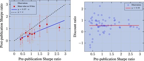
We describe the post-publication performance drop in figure 1. We plot in the left (resp. right) panel the post-publication Sharpe ratio (resp. the discount ratio) as a function of the pre-publication Sharpe ratio. In line with McLean and Pontiff (2016), both charts confirm that, on average, post-publication Sharpe ratios are below the in-sample ones. The binscatter plot in the left panel (in red) indicates that, on average, the post-publication Sharpe ratio drops by 43%. This drop is a bit smaller than the one found in McLean and Pontiff (2016), where a 58% drop is reported. Their set of anomalies is slightly larger than ours and we use a different hedging technique, but the magnitude is reassuringly similar. The decay by a factor of two is consistent with the calibrated model of overfitting in Rej et al. (2019).

Figure 1. Left panel: Sharpe ratios of factors post-publication versus pre-publication. The regression is performed with OLS and has a $R^2$ of 67%. Observations are divided into deciles and we compute the average (resp. median) Sharpe ratio in-sample (resp. post-publication). The error bars show the standard deviation in the y direction. Right panel: Discount ratio versus pre-publication Sharpe ratio. The median discount ratio is 0.55.

3.3. Performance drop on liquid stocks

We now study the out-of-sample performance drop when restricting the pool of stocks. All of the replicated anomalies are defined so far on a subset of the CRSP universe where penny stocks and delistings are discarded, but which still include many very small caps that cannot be traded at scale. Pools of larger stocks are more relevant for asset managers looking for capacity, while academic research has for long been focused on rejecting non-predictability of stock returns.

In this section, our test consists of looking at the performance on two of these larger pools: a pool made of 1000 most liquid stocks of CRSP and a one made of 500 most liquid names. The notion of ‘out-of-sample’ test here is an abuse of language as these pools are actually a small subsample of the original in-sample pool. But these pools were not the ones used by researchers when looking for predictability.

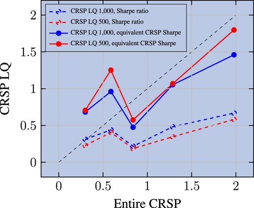
We plot in figure 2 Sharpe ratios on these subpools against the Sharpe ratios on CRSP. Clearly, Sharpe ratios on large caps are smaller than original in-sample Sharpe ratios (the dashed lines are below the 45-degree line). A naive reading of this result would be that the performance drops significantly in subsamples that have not been the main focus of researchers.

Figure 2. Raw and size-adjusted Sharpe ratios on liquidity pools vs. their original pool (as specified by the authors) counterparts. Observations are cut into five bins based on quantiles, we then compute the average (resp. median) Sharpe ratio on CRSP (resp. CRSP LQ 1000 or 500). Factors are beta-neutralised and Sharpe ratios below 0.3 on the entire CRSP universe (in-sample) are excluded.

But by design the pools of liquid stocks have a much smaller number of stocks than CRSP universe researchers are working with, so a size adjustment as described in section 3.1 is in order. We define the adjusted Sharpe as (5) $S{R}_p^{\ast }:=S{R}_p\sqrt{\frac{N_{CRSP}}{N_p}},$(5) where $S{R}_p^{\ast }$ is the Sharpe ratio on pool p adjusted for size. $S{R}_p$ is the Sharpe ratio computed on pool p and $N_p$ is the average number of stocks in this pool. Similarly, $N_{CRSP}$ is the average number of stocks in CRSP.

As discussed previously, the implicit assumption in equation (5(5) $S{R}_p^{\ast }:=S{R}_p\sqrt{\frac{N_{CRSP}}{N_p}},$(5) ) is that Sharpe ratios are directly proportional to $\sqrt{N}$, i.e. that predictability is a pure arbitrage, so that the Sharpe ratio would be infinite for $N\to \mathrm{\infty }$. Another key assumption we are making here is that the number of stocks in each pool is constant and well approximated by the average number of stocks in the pool over the period. This assumption is a very rough approximation of reality for CRSP, where number of stocks peaked just before 2000 and has declined ever since.

The solid lines of figure 2 report the result of this size adjustment. Now, the equivalent Sharpe ratio is much closer to the one computed on CRSP, even if on average still below the 45-degree line, hinting at a slight drop in performance out of sample. We can quantify the average decay by regressing the size adjusted Sharpe on the CRSP Sharpe for each one of the two pools separately. We report regression results in appendix table A2. We find that the Sharpe decay is 33% for the largest 1000 stocks, and 20% for the largest 500.

3.4. International evidence

We now analyze the performance drop on international pools of stocks. The rationale here is that most published anomalies were identified using US data only and were not initially tested on foreign stocks—a reason for this is the absence of international stock returns in WRDS, the platform most finance academics use. Several papers (see for instance Asness et al. 2013, Griffin 2015, Lu et al. 2017) have looked at the robustness of a small number of well-known factors outside of the USA, but papers investigating large set of factors (like McLean and Pontiff 2016, Hou et al. 2018) typically focus on US data. An exception is Jacobs and Müller (2020), who look at a large set of factors (241) in 39 stock markets. Another data advantage of their paper compared to ours is that they can observe returns before and after publication—in our case, our international data are mostly after publication. Unlike them, however, we focus on Sharpe ratios to appraise predictability rather than on t-stats.

We explore how well our 72 factors fare on pools of stocks from China, Hong Kong, Korea, Japan, Australia, Continental Europe, UK and Canada. We complement this list with the Russell 1000 and Russell 3000, which are broad indices of US stocks. All these pools correspond to well-known and liquid stock indices popular among large global investors. The period of study is shorter than that for CRSP because of limited historical data.

To measure performance in these pools, a size adjustment is necessary, as international pools are in general much smaller than the CRSP universe. Figure A1 shows the variation over time of the number of stocks in each one of these pools. Most of these indices—except the China SE Shanghai Composite—have a reasonably stable number of stocks. But more importantly, all of them are smaller than CRSP, some of them much smaller (the Australian pool has only 200 stocks) thus underlining the importance of the size adjustment.

Table 3 reports the results. Each line corresponds to a pool of stocks. We show the discount ratios, as defined in equation (1(1) $q:=\frac{S{R}_{OOS}}{S{R}_{IS}},$(1) ). Sharpe ratios are computed raw (column 4) and using the two pool size adjustments described in section 3.3. Given that all pools are much smaller than the US, size adjustments make a big difference. Across the eight international pools, the discount ratio is close to $.4$, a number similar but slightly smaller to what is obtained by comparing pre- and post-publication Sharpe on CRSP. Thus the Sharpe decay is significant but not complete for our set of 72 factors.

Table 3. Median discount ratio.

				Size adjusted
Country	Index/pool	Average size	Raw	Simple	Complex
Panel A: US pools
United States	CRSP post-publication	4694	0.55	0.52	0.54
United States	Russell 3000 Index	2933	0.20	0.26	0.22
United States	Russell 1000 Index	975	0.17	0.37	0.32
Panel B: Non-US pools
Australia	S&P/ASX 200 Index	200	0.08	0.38	1.00
Europe	Bloomberg European 500	505	0.09	0.24	0.37
Hong Kong	Hang Seng Composite Index	312	0.20	0.75	0.74
Korea	Korea Kospi Index	734	0.20	0.52	0.44
China	China SE Shanghai Composite	918	0.18	0.39	0.32
Canada	S&P/TSX Composite Index	244	0.11	0.47	0.87
Japan	TOPIX 500 Index (TSE)	500	−0.01	−0.02	0.32
United Kingdom	FTSE 100 Index	100	0.08	0.53	1.78
Average non-US		439	0.11	0.41	0.73

‘Out-of-US’ Sharpe ratio decay is consistent with overfitting, but also with arbitrage, as for many of factors in our zoo the period under consideration falls after the publication date. Quantitative investors could have had time to learn about anomalies and implemented them globally. A third possibility is that some stock anomalies reflect US-specific mispricing (due to differences in economics forces or accounting norms for instance).

The rest of the paper tries to distinguish between these possibilities. Before moving to this discussion, let us compare our results with Jacobs and Müller (2020), who find that anomalous returns are also present in non-US markets, both before and after publication. There are key methodological differences between our approaches. First, they focus on anomaly returns, while we focus on risk-adjusted performance (Sharpe ratios). For instance, it could well be that risk-adjusted performance deteriorates after publication while returns remain the same. Second, we compare international stock Sharpe ratios to pre-publication US Sharpe ratios. To do this properly, we show that it is crucial to adjust for pool size to make things comparable. Since Jacobs and Müller (2020) are not looking at risk adjusted performance, no size adjustment is necessary in their case.

4. Predicting out-of-sample performance decay

The previous section has established that, whether we look at post-publication data, liquid US pools or international pools, we observe a sizable drop in Sharpe ratio compared to the original in-sample value. The question we address now is whether we can predict the Sharpe ratio decay using in-sample diagnostics. We will focus here on post-publication decay.

To construct these in-sample characteristics, we draw inspiration from the overfitting and arbitrage hypotheses. While we find that several variables succeed in explaining part of the discount ratios' cross-sectional variance, we are cognizant of the fact that we might have missed important (statistically significant) proxies in both sets.

4.1. Arbitrage covariates

We define four variables that are designed to test the potential influx of arbitrage capital into a strategy once it is published. All of these variables are defined such that the expected sign of their effect on the discount ratio is negative (larger values mean that arbitrage capital is expected to move in more aggressively after publication):

• Holding period. The longer the holding period of a given factor, the cheaper it is to trade it and thus the higher is its capacity (Bonelli et al. 2019). We thus expect that slower strategies attract more arbitrage capital than faster ones. As a result performance will decay more post-publication. Let us define the matrix $\mathit{\omega }=({\omega }_{t,s}{)}_{\begin{array}{c}0<t\le T\\ 0<s\le N\end{array}}$ of weights used to compute factor f. We compute the holding period of stock s as (6) ${\mathcal{H}}_s^f:=2\cdot \frac{\sqrt{〈{\mathit{\omega }}_s^2〉-〈{\mathit{\omega }}_s{〉}^2}}{〈\left|\mathrm{\Delta }{\mathit{\omega }}_s\right|〉},$(6) where $\mathrm{\Delta }{\mathit{\omega }}_s:=({\omega }_{t+1,s}-{\omega }_{t,s}{)}_{0<t<T}$ and $〈\cdot 〉$ denotes the mean operator. We define the holding period of factor f as the cross-sectional median: ${\mathcal{H}}^f:=M\left({\mathcal{H}}_s^f\right)$.

• Amihud's liquidity. As arbitrage capital moves in we expect it to have a preference for liquid stocks. If liquidity correlates with factor exposure, arbitrage will hurt out-of-sample performance more and reduce the discount rate. We use Amihud's definition of illiquidity (Amihud 2002) with a minus sign. Thus the liquidity of a stock s at day t is (7) $L_{s,t}:=-\frac{\left|r_{s,t}\right|}{V_{s,t}},$(7) with r the (daily) return and V the (daily) volume. We then compute the weighted average liquidity in the portfolio associated with factor f and compare it to the average pool liquidity: (8) $\begin{array}{rl}{\mathcal{L}}_t^f& :=\frac{1}{2}(\frac{\sum _{{\omega }_{s,t}>0}{\omega }_{s,t}{L}_{s,t}}{\sum _{{\omega }_{s,t}>0}{\omega }_{s,t}}+\frac{\sum _{{\omega }_{s,t}<0}{\omega }_{s,t}{L}_{s,t}}{\sum _{{\omega }_{s,t}<0}{\omega }_{s,t}})\\ & \cdot \frac{N}{\sum _s{L}_{s,t}}.\end{array}$(8) The liquidity of a factor is its time-series median ${\mathcal{L}}^f:=M\left({\mathcal{L}}_t^f\right)$.

• Portfolio market cap to average market cap ratio. This variable is a variant of the previous one, where liquidity is now proxied by firm size. If factor loadings are correlated with market capitalization, arbitrage capital will find it easier to move in and correct the mispricing. We construct this variable as the (weighted) average market cap in the long and short legs compared to the average market capitalization of all stocks in CRSP. With $E_{s,t}$ being the market cap of stock s at time t, let us define (9) $\begin{array}{rl}{\mathcal{M}}_t^f& :=\frac{1}{2}(\frac{\sum _{{\omega }_{s,t}>0}{\omega }_{s,t}{E}_{s,t}}{\sum _{{\omega }_{s,t}>0}{\omega }_{s,t}}+\frac{\sum _{{\omega }_{s,t}<0}{\omega }_{s,t}{E}_{s,t}}{\sum _{{\omega }_{s,t}<0}{\omega }_{s,t}})\\ & \cdot \frac{N}{\sum _s{E}_{s,t}}.\end{array}$(9) We take the time-series median as the final measure ${\mathcal{M}}^f:=M\left({\mathcal{M}}_t^f\right)$. Hence, large values of this proxy suggest an exposure to large, liquid stocks and thus we expect a lower discount ratio.

• Short leg market cap ratio. This variable is a variant of the previous one designed to capture the hard-to-borrow effect. It is based on the idea that small stocks may be very costly to short. We define this variable as the (weighted) average market cap in the short leg relative to the average market cap of the market. If the ratio is large, the short leg is cheap to implement and arbitrage capital is expected to move in aggressively (table 4).

Table 4. Statistics for arbitrage variables before standardization. We only retain strategies with an in-sample Sharpe ratio on CRSP higher than 0.3.

	Mean	Median	$Q_1$	$Q_3$	$N$
log holding period	6.08	6.22	5.91	6.40	58
log mkt cap long short	0.88	0.62	−0.08	2.00	58
log mkt cap short	0.95	0.66	0.04	1.64	58
liquidity	−0.64	−0.74	−0.99	−0.17	58

Note: Log holding period is the natural logarithm of the factor's holding period. Log mkt cap long short is the natural logarithm of the ratio factor's market cap to average market cap. Log mkt cap short is defined as the natural logarithm of the ratio factor's short leg market cap to average market cap. Liquidity is the ratio of factor's liquidity (minus Amihud's liquidity) to average pool liquidity.

4.2. Overfitting covariates

We now propose proxies that may be relevant to multiple testing hypothesis. We use the same sign convention as for the arbitrage variables. We start with a variable that proxies for the fact that models may have been ‘selected’ to fit the data in-sample:

• Low t-stat. Harvey (2017) claims, drawing upon Bonferroni inequalities, that statistical significance in investment research requires a t-stat in excess of 3 to counteract the problem of multiple testing. Thus we construct a dummy variable equal to one if the t-stat of the factor is less than 3. When this is the case, the risk of multiple hypothesis testing is higher, and the expected discount ratio should be lower.

If there are many ways of testing the hypothesis, then, conditional on publication, we expect a larger drop of performance out-of-sample. We thus propose four variables that seek to capture the ‘flexibility’ of the sorting variable in achieving different in-sample Sharpe ratios:

• Log quantile span. We define a family of strategies for each given factor by varying the top and bottom quantiles used to define the long and short legs of the portfolio. For each quantile $q\in \{5\mathrm{\%},10\mathrm{\%},15\mathrm{\%},20\mathrm{\%},25\mathrm{\%},30\mathrm{\%},35\mathrm{\%}\}$, we compute one in-sample Sharpe $S{R}_q$. We then define this flexibility variable of factor f as (10) ${\mathcal{F}}^f:=\ln \frac{\sqrt{〈S{R}_q^2〉-〈S{R}_q{〉}^2}}{S{R}_{IS}}.$(10) The intuition is that the larger this variable is, the more sensitive is the factor's performance w.r.t. portfolio construction and the less likely it is to generalize outside the training period.

• Deviation from best q. This is a variation on the previous measure. Instead of log of the range, we look at the quantile $q^{\ast }$ that maximizes the in-sample Sharpe. We then compute the difference between $S{R}_{q^{\ast }}$ and the in-sample Sharpe in the baseline specification.

• Dummy number of Compustat items. We define this dummy variable as one if the number of Compustat items used to define the factor is more than two. The intuition behind this variable is that once researchers start combining multiple Compustat items the number of possible combinations increases exponentially and some of them will lead to false positive signals in-sample. Let us point out though that sometimes authors use several Compustat items to define certain well-known financial/accounting metrics not directly available as Compustat items. This weakens our argument only slightly, as a raft of accounting metrics exists thus considerably extending the universe of possible false positives.

• Dummy number of operations. This dummy variable is equal to one if the number of operations used to define the factor is more than two. The intuition is similar to the number of Compustat items. More complexity increases the scope for in-sample overfitting.

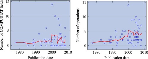
In figure 3, we show that there is a tendency to introduce more and more complexity in research. The trend towards increasing complexity may just reflect that more complex formulas are needed to find new signals or plain overfitting. Our cross-sectional analysis below investigates this.

Figure 3. Number of Compustat fields (resp. operations) used to compute the factors' characteristic, as a function of publication date. We only show factors whose in-sample Sharpe ratio is greater than 0.3. One dot per factor. The red line represents a moving average of five factors.

The last set of variables probes small-sample sensitivity of in-sample Sharpe estimates.

• Minus number of months in-sample. Backtests over long periods are more likely to pick up ‘stationary’ anomalies. Such persistent anomalies should have a higher chance of working outside the training period. Besides, even if all stock phenomena were to be stationary, it is easier to ‘mine’ statistically significant relationships on a short sample. Thus if this variable is larger, we expect the discount ratio to be smaller.

• Log of subset std. This variable captures the robustness of the factor strategy to removal of a small subset of stocks. To this effect, we draw a 10% random subset of stocks every period. We drop this subset and calculate the Sharpe ratio on the remaining 90% of the sample. We repeat this step 100 times and compute the standard deviation of Sharpe ratios. This variable captures the sensitivity of a factor's performance to removing a small number of observations. If this sensitivity is high, then the in-sample Sharpe is more likely to depend on a small subset of stocks that may exhibit different properties out-of-sample or disappear from the pool altogether.

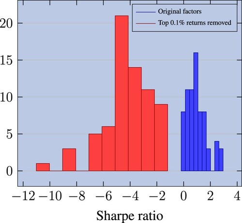
• Diff SR with dropped data. With this variable, we seek to capture the contribution of outliers to the in-sample Sharpe ratio. Such outliers are potentially important since returns are known to be non-normal (see e.g. Gabaix 2016). To appraise their contribution to the in-sample Sharpe ratio, we implement the methodology proposed by Broderick et al. (2021). We redefine the factors in such a way as to remove the 0.1% observations that are most impactful. Following the definition of Broderick et al., these observations are the top 0.1% portfolio returns throughout the entire period.² Since our factors are defined in a long/short way, these may came either from the long or the short leg. Once this has been done, we recompute the in-sample Sharpe. In figure 4, we report the distribution of Sharpe ratios of baseline strategies and Sharpe ratios after the 0.1% trimming. This figure illustrates the very large difference between the data and the trimmed data. After removing the top 0.1% contributors, the mean of the Sharpe ratio distribution drops from +1 to −4. This is in line with stock returns not being Gaussian. Classic anomalies rely on a very small sample of extreme contributors. The difference between the new Sharpe ratio and the original one is our variable. The larger it is, the more the in-sample performance is sensitive to a few stocks. We thus expect performance to drop more out-of-sample.

Figure 4. Distribution of in-sample Sharpe ratios of factors. We show original factors and a version where we remove the top 0.1% portfolio returns (Broderick et al. 2021). All 72 factors are beta-neutralised.

To make these variables comparable to one another, we standardize them, so that all have a mean of zero and a standard deviation of one (table 5).

Table 5. Stats for overfitting variables before standardization. We only retain strategies with an in-sample Sharpe ratio on CRSP higher than 0.3.

	Mean	Median	$Q_1$	$Q_3$	$N$
dummy tstat	0.28	0.00	0.00	1.00	60
log q span cv	−1.95	−2.11	−2.43	−1.37	58
diff from best q	0.15	0.08	0.03	0.21	58
dummy nb fields	0.35	0.00	0.00	1.00	60
dummy nb operations	0.75	1.00	0.75	1.00	60
sqrt nb months is	−16.06	−16.57	−18.52	−12.64	60
log std subset	−3.41	−3.45	−3.82	−2.91	57
diff w drop data	5.42	5.35	4.34	6.42	58

Note: Dummy tstat equals 1 (resp. 0) if the factor's t-stat is less (resp. greater) than 3. Log q span cv is the natural logarithm of the coefficient of variation of the factor's SR when varying the top and bottom quantiles that defines long/short legs. Diff from best q is the difference between the maximal in-sample SR (by varying the quantiles) and the original in-sample SR. Dummy nb fields equals 1 (resp. 0) if the number of Compustat variables to define the factor is greater or equal (resp. less) than 2. Dummy nb operations equal 1 (resp. 0) if the number of operations to define the factor is greater or equal (resp. less) than 2. Sqrt nb months is minus the square root of number of months used in the back test of the factor. Log std subset is the natural logarithm of the standard deviation of SR when removing a random 10% of stocks. Diff w drop data is the difference between the original in-sample SR and the SR when removing the top 0.1% portfolio returns.

4.3. Publication date

Our 11th variable is the publication date, potentially a proxy for both arbitrage and overfitting. The date of publication is measured in Unix time, i.e. the number of seconds that have elapsed since Jan 1st 1970. We expect the publication year to negatively affect discount ratios, under both the arbitrage and the overfitting views. According to the overfitting view, as the ‘true’ factors are revealed by researchers, people try harder and harder to come up with new strategies. Under the arbitrage view, given the rise of systematic investment over the past few decades, a reasonable conjecture would be that arbitrage capital is more likely to ‘rush in’ after publication than before.

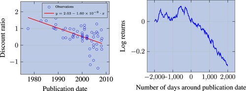
Consistent with both of these views, the left panel in figure 5 shows that Sharpe ratio decay after publication has increased substantially over time, especially since 2000.³ This change has happened fast, with the discount ratio decreasing by 0.05 every year. In the right panel of figure 5, we show the average detrended PnL of strategies around the date of publication, ranging from 2000 days before to 2000 days after. For each strategy, the PnL is calculated as the cumulative return of investing one dollar in the risk-controlled strategy. The detrended PnL is computed by removing the PnL mean in the pre-publication period. The right panel clearly shows a very fast performance decay after publication (actually starting around 1 year and a half before the publication date, which is consistent with pre-print circulation). This suggests that performance decays extremely fast, possibly too fast to be explained by arbitrage capital inflows.

Figure 5. Left panel: discount ratio as a function of publication date. Factors are beta-neutralised and computed on CRSP and we only retain those with Sharpe ratio greater than 0.3; one dot per factor; the red line draws a linear trend, fitted on blue dots, where dates are represented in Unix time. Right panel: average PnL of factors, centered on publication date; the average PnL is detrended based on the pre-publication period; factors are market-neutralised and, to be comparable, risk-managed; we use with the original stock pool and eliminate strategies that do not replicate well in sample.

4.4. Regression results

Given the rather small size of our sample of anomalies, we start with univariate regressions results. This helps to identify relevant variables and avoids the pitfalls of collinearity. In table A3, we present correlations between arbitrage variables. We see that three of our covariates: log mkt cap long short, log mkt cap short and illiquidity, are highly correlated. This is to be expected as they all proxy for effects that are related to liquidity.

Table 6 reports the results of the univariate regressions on each of the liquidity proxies. As expected, all coefficients are negative. The market cap based coefficients are both significant, as is the Amihud-liquidity-based one. We conclude that limited market liquidity prevent some of the market inefficiencies from being completely arbitraged away.

Table 6. OLS univariate regressions of the discount ratio on arbitrage variables (t-stats in parentheses).

	1	2	3	4
const	0.87	0.70***	0.72***	0.36***
	(1.22)	(7.8)	(7.86)	(2.64)
log holding period	−0.05
	(−0.41)
log mkt cap long short		−0.14**
		(−2.48)
log mkt cap short			−0.15***
			(−2.67)
liquidity				−0.34*
				(−1.95)
N	58	58	58	58
$R^2$	0.00	0.10	0.11	0.06

Note: ${}^{\ast \ast \ast }p<0.01$; ${}^{\ast \ast }p<0.05$; ${}^{\ast }p<0.1$

We now move to overfitting variables. In table A4, we present the correlations between overfitting variables. Much of the correlation structure does not come as a surprise. The correlation between dapublished and sqrt nb months is mechanical. The correlation between dapublished and number of operations is not mechanical, but still intuitive. With time authors explored more complex characteristics, as shown in figure 3.

Regression results are provided in table 7. The statistically significant overfitting variables capture different overfitting-related effects, as it may be inferred from lower level of correlations between them. First, publication date emerges as a very strong predictor of post-publication Sharpe ratio decay. As seen in figure 5 factors published more recently tend to be more overfitted. Second, among the ‘flexibility’ variables, the number of operations is the only one that comes out significant, although, as expected, all are negative. Finally, the two measures that seek to capture the dependence on a small number of observations do well at explaining the cross-section of Sharpe ratio decays. Anomalies that derive a significant part of their performance in-sample from a small subset of stocks tend to experience a more pronounced drop of risk-adjusted performance. Our measure of sensitivity to removal of a randomly-chosen 10% of the original sample also strongly predicts performance decay.

Table 7. OLS univariate regressions of the discount ratio on overfitting variables (t-stats in parentheses).

	1	2	3	4	5
const	0.59${}^{\ast \ast \ast }$	0.52${}^{\ast \ast \ast }$	0.54${}^{\ast \ast \ast }$	0.63${}^{\ast \ast \ast }$	0.92${}^{\ast \ast \ast }$
	(6.12)	(6.09)	(6.39)	(6.29)	(5.9)
dummy tstat	−0.15
	(−0.8)
log q span cv		−0.10
		(−1.08)
diff from best q			−0.07
			(−0.83)
dummy nb fields				−0.23
				(−1.37)
dummy nb operations					−0.49${}^{\ast \ast \ast }$
					(−2.72)
N	60	58	58	60	60
$R^2$	0.01	0.02	0.01	0.03	0.11
const	0.55${}^{\ast \ast \ast }$	0.59${}^{\ast \ast \ast }$	0.59${}^{\ast \ast \ast }$	0.53${}^{\ast \ast \ast }$
	(6.73)	(8.01)	(7.99)	(7.72)
sqrt nb months is	0.08
	(0.91)
log std subset		−0.16${}^{\ast \ast }$
		(−2.04)
diff w drop data			−0.21${}^{\ast \ast \ast }$
			(−2.99)
dapublished				−0.35${}^{\ast \ast \ast }$
				(−5.06)
N	60	57	58	60
$R^2$	0.01	0.07	0.14	0.31

Note: ${}^{\ast \ast \ast }p<0.01$; ${}^{\ast \ast }p<0.05$; ${}^{\ast }p<0.1$.

Overall, date of publication, the sensitivity to outliers suggested by Broderick et al. (2021) and the number of operations have the largest univariate $R^2$, i.e..30, .14 and .11. Put together, the three variables have an $R^2$ of 0.36, essentially driven by the first two variables.

4.5. Putting it all together

Last, we run a horse race between arbitrage and overfitting variables. We construct two variables: ‘arbitrage vulnerability’ and ‘overfitting vulnerability’, by taking an arithmetic mean for each set. Recall that all variables have been standardized to an s.d. of 1 and a mean of 0, so taking a mean gives an equal weight to all co-variates. To these two summary variables, we add the publication date.

In table 8, we report the result of the predictive regression. First, the date of publication has a strong explanatory power on the cross-section of Sharpe decays, with an $R^2$ of 0.30. Second, the combined overfitting vulnerability variable is also quite strong, with an $R^2$ of .15. Arbitrage vulnerability has a weaker predictive power and a lower—yet significant—t-stat. When we put the three variables together we end up with an $R^2$ of .47. Removing the arbitrage variable diminishes the $R^2$ only slightly suggesting its marginal importance.

Table 8. OLS regressions with arbitrage and overfitting vulnerabilities.

	Discount ratio
Dependent variable:	1	2	3	4	5	6
Year of publication −1990	−.05${}^{\ast \ast \ast }$				−.041${}^{\ast \ast \ast }$	−.044${}^{\ast \ast \ast }$
	(−4.9)				(−4.9)	(−5.2)
Arbitrage vulnerability		−.28${}^{\ast \ast }$		−.21${}^{\ast \ast }$	−.13
		(−2.6)		(−2.1)	(−1.5)
Overfitting vulnerability			−.34${}^{\ast \ast \ast }$	−.28${}^{\ast \ast }$	−.28${}^{\ast \ast \ast }$	−.31${}^{\ast \ast \ast }$
			(−3.1)	(−2.5)	(−3)	(−3.5)
Constant	1${}^{\ast \ast \ast }$	.58${}^{\ast \ast \ast }$	.55${}^{\ast \ast \ast }$	.55${}^{\ast \ast \ast }$	.92${}^{\ast \ast \ast }$	.94${}^{\ast \ast \ast }$
	(8.7)	(7.7)	(7.4)	(7.7)	(9.6)	(9.8)
N	60	58	55	55	55	55
$R^2$	0.30	0.11	0.15	0.19	0.47	0.45

Note: ${}^{\ast \ast \ast }p<0.01$; ${}^{\ast \ast }p<0.05$; ${}^{\ast }p<0.1$.

5. Conclusion

In this article, we confirm that published anomalies tend to deliver about 50% of the in-sample performance when evaluated outside of the sample. Unlike previous studies of this kind, we focus on risk-adjusted performance, rather than returns or t-stats. This novel emphasis requires that we develop new adjustments for pool size due to important diversification effects.

The other key innovation of our study is the analysis of covariates that (1) can be computed in-sample and (2) may predict the post-publication performance decay. To build these covariates, we rely on two hypotheses put forth in the literature: overfitting and arbitrage. We find that publication date, sensitivity to small sample bias, and formula complexity jointly explain some 30% of the cross-sectional variation in performance decay.

Acknowledgements

We thank Yves Lemperière, Philip Seager, Mark Potters and Jean-Philippe Bouchaud for helpful feedback.

Notes

1 See Harvey et al. (2015), McLean and Pontiff (2016), Hou et al. (2018), Chen and Zimmerman (2020), and Jensen et al. (2021) among others.

2 More precisely, each stock contributes ${\omega }_{s,t}{r}_{s,t+1}$ to the strategy P&L every month. We drop the top 0.1% contributions.

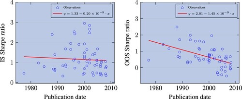
3 This comes from the decay of out-of-sample Sharpe ratio, while the in-sample Sharpe stays flat on average with publication date. See figure A2.

Appendices

Appendix 1. Tables

Table A1. List of factors and the corresponding references.

Factor	Reference article
Price earnings	Basu (1977)
Unexpected quarterly earnings	Rendleman et al. (1982)
Long term reversal	De Bondt and Thaler (1985)
Debt equity	Bhandari (1988)
Change in inventory-to-assets	Ou and Penman (1989)
Change in dividend per share	Ou and Penman (1989)
Change in capital expenditures-to-assets	Ou and Penman (1989)
Return on total assets	Ou and Penman (1989)
Debt repayment	Ou and Penman (1989)
Depreciation-to-PP&E	Holthausen and Larcker (1992)
Change in depreciation-to-PP&E	Holthausen and Larcker (1992)
Change in total assets	Holthausen and Larcker (1992)
Size	Fama and French (1993)
Book-to-market	Fama and French (1993)
Momentum	Jegadeesh and Titman (1993)
Sales growth	Lakonishok et al. (1994)
Cash flow-to-price	Lakonishok et al. (1994)
Working capital accruals	Sloan (1996)
Sales-to-price	Barbee et al. (1996)
Share turnover	Haugen and Baker (1996)
Cash flow-to-price variability	Haugen and Baker (1996)
Trading volume trend	Haugen and Baker (1996)
Inventory	Abarbanell and Bushee (1998)
Gross margin	Abarbanell and Bushee (1998)
Capital expenditures	Abarbanell and Bushee (1998)
Industry momentum	Moskowitz and Grinblatt (1999)
F-score	Piotroski (2000)
Industry adjusted book-to-market	Asness et al. (2000)
Industry adjusted cash flow-to-price	Asness et al. (2000)
Industry adjusted size	Asness et al. (2000)
Industry adjusted momentum	Asness et al. (2000)
Industry adjusted long term reversal	Asness et al. (2000)
Industry adjusted short term reversal	Asness et al. (2000)
Dollar volume	Chordia et al. (2001)
Dollar volume coefficient of variation	Chordia et al. (2001)
Share turnover coefficient of variation	Chordia et al. (2001)
Change in inventory	Thomas and Zhang (2002)
Change in current assets	Thomas and Zhang (2002)
Depreciation	Thomas and Zhang (2002)
Change in accounts receivable	Thomas and Zhang (2002)
Other accruals	Thomas and Zhang (2002)
Illiquidity	Amihud (2002)
Liquidity	Pástor and Stambaugh (2003)
Idiosyncratic return volatility x book-to-market	Ali et al. (2003)
Price x book-to-market	Ali et al. (2003)
Operating cash flow-to-price	Desai et al. (2004)
Abnormal corporate investment	Titman et al. (2004)
Accrual quality	Francis et al. (2004)
Earnings persistence	Francis et al. (2004)
Smoothness	Francis et al. (2004)
Value relevance	Francis et al. (2004)
Timeliness	Francis et al. (2004)
Tax income-to-book income	Lev and Nissim (2004)
Price delay	Hou and Moskowitz (2005)
Firm age	Jiang et al. (2005)
Duration	Jiang et al. (2005)
Change in current operating assets	Richardson et al. (2005)
Change in non-current operating liabilities	Richardson et al. (2005)
Growth in capital expenditures	Anderson and Garcia-Feijoo (2006)
Growth in capital expenditures (alternative)	Anderson and Garcia-Feijoo (2006)
Low volatility	Ang et al. (2006)
Low beta ΔVIX	Ang et al. (2006)
Zero trading days	Liu (2006)
Composite issuance	Daniel and Titman (2006)
Intangible return	Daniel and Titman (2006)
Earnings surprises x revenue surprises	Jegadeesh and Livnat (2006)
Industry concentration	Hou and Robinson (2006)
Change in shares outstanding	Pontiff and Woodgate (2008)
Seasonality	Heston and Sadka (2008)
Investment	Lyandres et al. (2008)
Investment growth	Xing (2007)
Change in asset turnover	Soliman (2008)

Table A2. OLS regressions of equivalent Sharpe ratio of CRSP LQ 500 (resp. 1000) on CRSP (t-stats in parenthesis).

	CRSP LQ 500	CRSP LQ 1000
coef	0.80${}^{\ast \ast \ast }$	0.67${}^{\ast \ast \ast }$
	(8.68)	(8.52)
N	60	60
$R^2$	0.56	0.55

Note: ${}^{\ast \ast \ast }p<0.01$; ${}^{\ast \ast }p<0.05$; ${}^{\ast }p<\mathrm{0.1.}$

Table A3. Correlation matrix for arbitrage variables.

	log holding period	log mkt cap long short	log mkt cap short	liquidity
log holding period	1.00
log mkt cap long short	−0.23	1.00
log mkt cap short	−0.08	0.89	1.00
liquidity	−0.07	0.78	0.62	1.00

Table A4. Correlation matrix for overfitting variables; dts = dummy tstat, lqscv = log q span cv, dbq = diff from best q, dnf = dumy nb fields, dno = dummy nb operations, snm = sqrt nb months is, lss = log std subset, ddd = diff w drop data.

	dts	lqscv	dbq	dnf	dno	snm	lss	ddd	dp
dts	1.00
lqscv	0.58	1.00
dbq	0.03	0.16	1.00
dnf	0.13	0.06	−0.02	1.00
dno	0.03	−0.07	0.06	0.23	1.00
snm	0.26	−0.05	−0.09	0.22	0.17	1.00
lss	0.14	0.16	0.00	0.44	0.43	0.48	1.00
ddd	−0.05	0.05	−0.05	0.24	0.35	0.22	0.48	1.00
dp	−0.11	0.14	0.09	0.09	0.29	−0.54	−0.04	0.27	1.00

Appendix 2. Figures

Figure A1. Number of constituents in each pool.

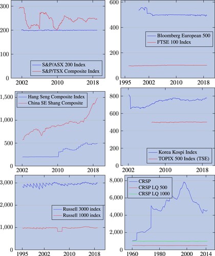
Figure A2. In-sample (resp. out-of-sample) Sharpe ratio as a function of publication date. Factors are beta-neutralised and computed on CRSP, conditional on its in-sample Sharpe ratio being greater than 0.3. One dot per factor. The red line draws a linear trend, fitted on blue dots, where dates are represented in Unix time. The $R^2$ are 0.4% and 24% respectively.

References

- Abarbanell, J.S. and Bushee, B.J., Abnormal returns to a fundamental analysis strategy. Account Rev., 1998, 73(1), 19–45. http://www.jstor.org/stable/248340.
- Ali, A., Hwang, L.S. and Trombley, M.A., Arbitrage risk and the book-to-market anomaly. J. Financ. Econ., 2003, 69(2), 355–373. doi:10.1016/S0304-405X(03)00116-8
- Amihud, Y., Illiquidity and stock returns: Cross-section and time-series effects. J. Financ. Markets, 2002, 5(1), 31–56. doi:10.1016/S1386-4181(01)00024-6
- Anderson, C.W. and Garcia-Feijoo, L., Empirical evidence on capital investment, growth options, and security returns. J. Finance, 2006, 61(1), 171–194. doi:10.1111/j.1540-6261.2006.00833.x
- Ang, A, Hodrick, R.J., Xing, Y. and Zhang, X., The cross-section of volatility and expected returns. J. Finance, 2006, 61(1), 259–299. doi:10.1111/j.1540-6261.2006.00836.x
- Asness, C.S., Porter, R.B. and Stevens, R.L., Predicting stock returns using industry-relative firm characteristics. 2000. doi:10.2139/ssrn.213872.
- Asness, C.S., Moskowitz, T.J. and Pedersen, L.H., Value and momentum everywhere. J. Finance, 2013, 68(3), 929–985. doi:10.1111/jofi.12021
- Barbee, W.C., Mukherji, S and Raines, G.A., Do sales–price and debt–equity explain stock returns better than book–market and firm size? Financ. Anal. J., 1996, 52(2), 56–60. doi:10.2469/faj.v52.n2.1980
- Basu, S., Investment performance of common stocks in relation to their price-earnings ratios: A test of the efficient market hypothesis. J. Finance, 1977, 32(3), 663–682. doi:10.1111/j.1540-6261.1977.tb01979.x
- Bhandari, L.C., Debt/equity ratio and expected common stock returns: Empirical evidence. J. Finance, 1988, 43(2), 507–528. doi:10.1111/j.1540-6261.1988.tb03952.x
- Bonelli, M., Landier, A., Simon, G. and Thesmar, D., The capacity of trading strategies. Tech. Rep. FIN-2015-1089, HEC Paris Research, 2019. http://doi.org/10.2139/ssrn.2585399.
- Broderick, T., Giordano, R. and Meager, R., An automatic finite-sample robustness metric: When can dropping a little data make a big difference? 2021, arXiv preprint. https://arxiv.org/abs/2011.14999.
- Brodeur, A., Lé, M., Sangnier, M. and Zylberberg, Y., Star wars: The empirics strike back. Amer. Econom. J. Appl. Econ., 2016, 8(1), 1–32. doi:10.1257/app.20150044
- Chen, A. and Zimmerman, T., Publication bias and the cross-section of stock returns. Finance and Economics Discussion Series 2018-033, 2018, Washington: Board of Governors of the Federal Reserve System. doi:10.17016/FEDS.2018.033.
- Chen, A. and Zimmerman, T., Open source cross-section asset pricing, 2020. doi:10.2139/ssrn.3604626.
- Chordia, T., Subrahmanyam, A. and Anshuman, V., Trading activity and expected stock returns. J. Financ. Econ., 2001, 59(1), 3–32. doi:10.1016/S0304-405X(00)00080-5
- Daniel, K. and Titman, S., Market reactions to tangible and intangible information. J. Finance, 2006, 61(4), 1605–1643.doi:10.1111/j.1540-6261.2006.00884.x
- De Bondt, W.F.M. and Thaler, R., Does the stock market overreact?. J. Finance, 1985, 40(3), 793–805. doi:10.1111/j.1540-6261.1985.tb05004.x
- Desai, H., Rajgopal, S. and Venkatachalam, M., Value–Glamour and accruals mispricing: One anomaly or two? Accounting Rev., 2004, 79(2), 355–385. doi:10.2308/accr.2004.79.2.355
- Fama, E.F. and French, K.R., Common risk factors in the returns on stocks and bonds. J. Financ. Econ., 1993, 33(1), 3–56. doi:10.1016/0304-405X(93)90023-5
- Francis, J., LaFond, R., Olsson, P.M. and Schipper, K., Costs of equity and earnings attributes. Accounting Rev., 2004, 79(4), 967–1010. doi:10.2308/accr.2004.79.4.967
- Gabaix, X., Power laws in economics: An introduction. J. Econ. Perspectives, 2016, 30(1), 185–206. doi:10.1257/jep.30.1.185
- Giglio, S., Liao, Y. and Xiu, D., Thousands of alpha tests. Rev. Financ. Stud., 2020, 34(7), 3456–3496. doi:10.1093/rfs/hhaa111
- Griffin, J., Are the fama and french factors global or country specific? Rev. Financ. Stud., 2015, 15(3), 783–803. doi:10.1093/rfs/15.3.783
- Haddad, V., Kozak, S. and Santosh, S., Factor timing. Rev. Financ. Stud., 2020, 33(5), 1980–2018. doi:10.1093/rfs/hhaa017
- Harvey, C.R., Presidential address: The scientific outlook in financial economics. J. Finance, 2017, 72(4), 1399–1440. doi:10.1111/jofi.12530
- Harvey, C.R., Liu, Y. and Zhu, H., …and the cross-section of expected returns. Rev. Financ. Stud., 2015, 29(1), 5–68. doi:10.1093/rfs/hhv059
- Haugen, R.A. and Baker, N.L., Commonality in the determinants of expected stock returns. J. Financ. Econ., 1996, 41(3), 401–439. doi:10.1016/0304-405X(95)00868-F
- Heston, S.L. and Sadka, R., Seasonality in the cross-section of stock returns. J. Financ. Econ., 2008, 87(2), 418–445. doi:10.1016/j.jfineco.2007.02.003
- Holthausen, R.W. and Larcker, D.F., The prediction of stock returns using financial statement information. J. Accounting Econ., 1992, 15, 373–411. doi:10.1016/0165-4101(92)90025-W
- Hou, K. and Moskowitz, T.J., Market frictions, price delay, and the cross-section of expected returns. Rev. Financ. Stud., 2005, 18(3), 981–1020. doi:10.1093/rfs/hhi023
- Hou, K. and Robinson, D.T., Industry concentration and average stock returns. J. Finance, 2006, 61(4), 1927–1956. doi:10.1111/j.1540-6261.2006.00893.x
- Hou, K., Xue, C. and Zhang, L., Replicating anomalies. Rev. Financ. Stud., 2018, 33(5), 2019–2133. doi:10.1093/rfs/hhy131
- Jacobs, H. and Müller, S., Anomalies across the globe: Once public, no longer existent? J. Financ. Econ., 2020, 135(1), 213–230. doi:10.1016/j.jfineco.2019.06.004
- Jegadeesh, N. and Livnat, J., Revenue surprises and stock returns. J. Accounting Econ., 2006, 41(1), 147–171. doi:10.1016/j.jacceco.2005.10.003
- Jegadeesh, N. and Titman, S., Returns to buying winners and selling losers: Implications for stock market efficiency. J. Finance, 1993, 48(1), 65–91. doi:10.2307/2328882
- Jensen, T.I., Kelly, B.T. and Pedersen, L.H., Is there a replication crisis in finance? Working Paper 28432, National Bureau of Economic Research, 2021. doi:10.3386/w28432.
- Jiang, G., Lee, C.M.C. and Zhang, Y., Information uncertainty and expected returns. Rev. Accounting Stud., 2005, 10, 185–221. doi:10.1007/s11142-005-1528-2
- Kozak, S., Nagel, S. and Santosh, S., Interpreting factor models. J. Finance, 2018, 73(3), 1183–1223. doi:10.1111/jofi.12612
- Lakonishok, J., Shleifer, A. and Vishny, R.W., Contrarian investment, extrapolation, and risk. J. Finance, 1994, 49(5), 1541–1578. doi:10.1111/j.1540-6261.1994.tb04772.x
- Lev, B. and Nissim, D., Taxable income, future earnings, and equity values. Accounting Rev., 2004, 79(4), 1039–1074. doi:10.2308/accr.2004.79.4.1039
- Liu, W., A liquidity-augmented capital asset pricing model. J. Financ. Econ., 2006, 82(3), 631–671. doi:10.1016/j.jfineco.2005.10.001
- Lu, X., Stambaugh, R.F. and Yuan, Y., Anomalies abroad: Beyond data mining. NBER Working Papers 23809, National Bureau of Economic Research, Inc., 2017. doi:10.3386/w23809.
- Lyandres, E., Sun, L. and Zhang, L., The new issues puzzle: Testing the investment-based explanation. Rev. Financ. Stud., 2008, 21(6), 2825–2855. doi:10.1093/rfs/hhm058
- McLean, R.D. and Pontiff, J., Does academic research destroy stock return predictability? J. Finance, 2016, 71(1), 5–32. doi:10.1111/jofi.12365
- Moskowitz, T.J. and Grinblatt, M., Do industries explain momentum? J. Finance, 1999, 54(4), 1249–1290. doi:10.1111/0022-1082.00146
- Ou, J.A. and Penman, S.H., Financial statement analysis and the prediction of stock returns. J. Accounting Econ., 1989, 11, 295–329. doi:10.1016/0165-4101(89)90017-7
- Piotroski, J.D., Value investing: The use of historical financial statement information to separate winners from losers. J. Accounting Res., 2000, 38, 1–41. doi:10.2307/2672906
- Pontiff, J. and Woodgate, A., Share issuance and cross-sectional returns. J. Finance, 2008, 63(2), 921–945. doi:10.1111/j.1540-6261.2008.01335.x
- Pástor, L. and Stambaugh, R.F., Liquidity risk and expected stock returns. J. Polit. Econ., 2003, 111(3), 642–685. doi:10.1086/374184
- Rej, A., Seager, P. and Bouchaud, J.P., How should you discount your backtest PnL? Wilmott, 2019, 2019(103), 53–57. doi:10.1002/wilm.10793
- Rendleman, R.J., Jones, C.P. and Latané, H.A., Empirical anomalies based on unexpected earnings and the importance of risk adjustments. J. Financ. Econ., 1982, 10(3), 269–287. doi:10.1016/0304-405X(82)90003-4
- Richardson, S.A., Sloan, R.G., Soliman, M.T. and Tuna, I., Accrual reliability, earnings persistence and stock prices. J. Accounting Econ., 2005, 39(3), 437–485. doi:10.1016/j.jacceco.2005.04.005
- Sloan, R.G., Do stock prices fully reflect information in accruals and cash flows about future earnings? Account Rev., 1996, 71(3), 289–315. http://www.jstor.org/stable/248290.
- Soliman, M.T., The use of dupont analysis by market participants. Account. Rev., 2008, 83(3), 823–853. doi:10.2308/accr.2008.83.3.823
- Thomas, J.K. and Zhang, H., Inventory changes and future returns. Rev. Account. Stud., 2002, 7, 163–187. doi:10.1023/A:1020221918065
- Titman, S., Wei, K.C.J. and Xie, F., Capital investments and stock returns. J. Finan. Quant. Anal., 2004, 39(4), 677–700. doi:10.1017/S0022109000003173
- Xing, Y., Interpreting the value effect through the Q-theory: An empirical investigation. Rev. Financ. Stud., 2007, 21(4), 1767–1795. doi:10.1093/rfs/hhm051
- Yan, X.S. and Zheng, L., Fundamental analysis and the cross-section of stock returns: A data-mining approach. Rev. Financ. Stud., 2017, 30(4), 1382–1423. doi:10.1093/rfs/hhx001