Bitcoin: jumps, convenience yields, and option prices

Abstract

We investigate Bitcoin pricing characteristics and find evidence of jumps and positive convenience yield. We develop a theoretical jump diffusion model for options on spots and use simulations to evaluate non-linear parameter estimates. Data from the Deribit exchange is used to compare the performance of the jump diffusion models with Practitioner Black–Scholes models. Using Diebold–Marino statistics and standard error metrics, we find that the jump diffusion models significantly outperform Practitioner Black–Scholes models. We conclude that Bitcoin behaves more like a commodity than a currency.

Keywords:

• Bitcoin
• Options
• Jump-diffusion
• Parameter estimation commodity

1. Introduction

Bitcoin is a form of the peer-to-peer electronic cash system initially introduced by the pseudonymous Satoshi Nakamoto in 2008. Since the first inception of bitcoin in 2009, the market for cryptocurrencies built on blockchain technology has evolved dramatically. By November 2020, there are more than 7700 cryptocurrencies in existence, according to CoinMarketCap. Bitcoin remains the most popular cryptocurrency with a volatile market cap that exceeded $1 trillion in May of 2021.

The substantial increase in bitcoin trading has led to a surge in interest for bitcoin derivatives as an efficient tool for hedging and managing risk. While there is considerable interest in bitcoin derivatives research, relatively few papers study the stochastic properties of bitcoin and bitcoin derivatives pricing. Siu and Elliott (2020) study the pricing of bitcoin options using a SETAR-GARCH model. Hou et al. (2020) develop a bitcoin options pricing model that allows stochastic volatility with correlated jump options. In a similar paper, Cao and Celik (2021) model option prices assuming that the underlying process is a currency with constant interest rates and jump-diffusions. However, these studies do not test their models empirically using actual bitcoin option prices due to the lack of data. Several researchers utilize available data on options traded on unregulated exchanges and adopt artificial neural network approaches to price bitcoin options (Pagnottoni 2019, Li et al. 2019a). Cretarola et al. (2020) propose a stochastic model for the bitcoin price dynamics driven by market attention and develop a quasi-closed form for option price.

We make a novel contribution to the literature by deriving a model for pricing bitcoin European options admitting both jumps and stochastic convenience yield. We utilize an extensive data set from Deribit that includes 470,326 puts and 575,763 calls. Launched in 2016, Deribit is the first crypto exchange to offer bitcoin options and currently accounts for nearly 90 % of the total market in terms of the daily trading volume. Using Diebold–Marino statistics, we find that the jump-diffusion model with convenience yield (JDC) significantly outperforms the Black–Scholes Practitioner model at out-of-sample horizons 1, 2,…,15 days. This result holds for both puts and calls using both an absolute value and root mean square error metric (RMSE). We estimate that bitcoin has a positive average convenience yield of about 2.35 % per annum.

2. Background

Bitcoin has attracted the attention of financial economists as a virtual currency with the potential to disrupt existing payment systems and traditional currencies (Böhme et al. 2015). Unlike standard fiat currencies, bitcoin is not formally backed by a government or central authority, and its supply is controlled by a software algorithm. The bitcoin supply is preprogrammed to grow at a decreasing rate before reaching the limit of 21 million units. More than 18 million bitcoins are already mined to date, and the final coin is projected to be mined in around 2140. A non-technical review of bitcoin's principles and properties can be founded in Böhme et al. (2015).

A substantial part of early literature focused on the potential effects of bitcoin as a transaction mechanism and the implications for central banks and monetary policy (Evans 2014, Dwyer 2015, Weber 2016, Chiu and Koeppl 2017, Schilling and Uhlig 2019, Raskin and Yermack 2018). Baur and Dimpfl (2019) studied price discovery in bitcoin spot and futures markets.

Various empirical studies have shown that bitcoin prices and return dynamic are intrinsically complex, extremely volatile, and exhibit bubble-like behaviors (Hafner 2020, Cheah and Fry 2015). Many studies using different statistical methods have confirmed that bubble-like behavior, a dramatic price increase followed by an abrupt collapse, is a common and reoccurring characteristic of bitcoin price dynamics (Cheung et al. 2015, Chaim and Laurini 2019, Corbet et al. 2018, Li et al. 2019b, Waters and Bui 2022). Cretarola and Figà-Talamanca (2021) develop a continuous-time stochastic model for bitcoin price depending on a market attention factor and prove that bitcoin bubbles are fueled by market exuberance. That is, market attention drives bitcoin prices, and conversely, elevated price feeds sentiment in the same direction, creating a vicious loop that boosts bitcoin price into a bubble. Such price bubbles are detected in 2012–2013 and 2017, when the correlation between market attention and bitcoin returns exceeds a non-negative threshold. The efficiency of cryptocurrency markets has also been a controversial topic. While some studies have found that the cryptocurrency market is somehow efficient (Nadarajah and Chu 2017, Manahov and Urquhart 2021, Kang et al. 2022), a growing body of literature has documented inefficiencies in markets for bitcoin and arbitrage opportunities across exchanges (Krückeberg and Scholz 2020, Makarov and Schoar 2020, Pieters and Vivanco 2017, Shynkevitch 2020). Jo et al. (2020) have studied bitcoin as a high sentiment beta stock. See also Kyriazis et al. (2020) and references therein.

2.1. Bitcoin convenience yield

Even though bitcoin was introduced as a form of digital currency, financial economists have argued that it should be classified as a currency, a commodity, or a different asset class. Dyhrberg (2016) studies the similarities between gold, dollar and bitcoin prices and suggests that bitcoin has the same hedging capability. Given that its price is extremely volatile and almost exhibits no correlation with highly used currencies and gold, Yermack (2015) concludes that bitcoin's behaviors are more like a speculative investment than a currency. Utilizing bitcoin transaction data from July 2010 to June 2015, Baur et al. (2018) reach the same conclusion that bitcoin is mainly used as a speculative investment and not an alternative currency and medium of exchange. Recent studies that comprehensively examine the risks and returns conclude that bitcoin embraces an asset class that is fundamentally different from traditional asset classes (Liu and Tsyvinski 2018) and can be used for diversification and hedging purposes (Bouri et al. 2017, Krueckeberg and Scholz 2019, Borri 2019, Bianchi 2020). Virtual currencies such as Bitcoin, have been determined to be commodities under the Commodity Exchange Act (CEA). The IRS taxes bitcoin like other property (Internal Revenue Bulletin: 2014-21).

Similar to commodities, bitcoin provides a convenience yield. Convenience yield is a flow of benefits to owners of the spot not available to owners of corresponding futures contracts. For commodities, convenience yield is typically thought of as the extra benefit obtained from holding the physical commodity. The benefits of holding Bitcoin are not analogous to that of a physical commodity. Bitcoin is not a tangible asset and has no physical form, yet it provides streams of utility to its owners not found in futures contracts.

As a payment system, the benefits of owning bitcoin come from its uses to facilitate transactions, hedge hyper-inflation risk caused by political turmoil and serve as a store of value (Detzel et al. 2020). The secure, decentralized, and anonymous nature of bitcoin has made it popular as a medium for exchanges involving illicit goods and services (Athey et al. 2016, Barth et al. 2020). Illegal activities facilitated by bitcoin include money laundering, terrorism funding, illegal gambling and tax evasion. Yelowitz and Wilson (2015) use Google trends data to study bitcoin clientele and find that illegal activity is one of the main drivers of interest in bitcoin. Foley et al. (2019) use novel techniques for analyzing bitcoin user-level transactions and blockchain data to quantify the use of illicit trade facilitated by bitcoin. They find that approximately one-quarter of bitcoin users and almost one-half of bitcoin transactions are involved in illegal activities. They also note that the proportion of bitcoin activity associated with illegal trades has declined with increasing mainstream and speculative interest although the absolute amount has continued to grow.

Cong et al. (2020) develop a dynamic model of the platform economy and demonstrate that the cryptocurrency price is the present value of platform-specific convenience yield. Biais et al. (2020) also emphasize the fundamental value of Bitcoin from convenience yield reflecting transactional benefits. Kim (2021) finds that bitcoin has a positive convenience yield due in part to short-selling restrictions in the spot market and to network voting rights. Short selling pressures in spot markets increase the relative value of the spot vis á vis futures. The result is that the cost-of-carry model includes a positive convenience yield component. Bitcoin holders can also vote on network proposals to the bitcoin network with potential positive price effects. This is a right not afforded to holders of futures contracts.

Negative convenience is also possible due to the threat of unexpected regulation or other forms of government interference, hacking exposure, and lost passwords. Wu et al. (2021) use spot and futures data and a fractional cointegrated vector autoregressive model to document negative convenience yield. Their data, sourced from the Crypto.com Exchange and the Chicago Mercantile Exchange, are for the period from December 18, 2017, to July 31, 2020.

2.2. Jumps in bitcoin price

Several studies using daily data have documented sudden massive price swings in the form of jumps as important features of cryptocurrency dynamics. Chaim and Laurini (2018) find that jumps in bitcoin returns are contemporaneous and associated with formative events such as hack and unsuccessful fork attempts. Philippas et al. (2019) find that informative signals proxied by Google search volume and Twitter tweets partially drive bitcoin price and price jumps, especially under high uncertainty. Gronwald (2019) examines price movement in bitcoin and compares it with other exhaustible resource commodities such as gold and crude oil. While jumps in commodity prices are usually caused by short-run supply uncertainty, bitcoin faces no supply-side uncertainty due to its unique feature, implying that demand-side factors mainly cause jumps in bitcoin prices. Applying a non-parametric methodology, Kang and Kim (2019) find that jumps in bitcoin price tend to cluster during special periods and are independent of volatility. They suggest that market illiquidity caused erratic movements in bitcoin prices as more jumps are observed when trading volume is low. Using high-frequency transaction-level data from Mt.Gox, the leading bitcoin trading platform during 2011–2013, Scaillet et al. (2020) find that jumps in bitcoin price are more frequent than in US large-cap stocks. Similar to Kang and Kim's (2019) results, market illiquidity appears to be the main driving factor of price jumps. The lack of central authority to stabilize the market via circuit breakers or otherwise provide liquidity makes bitcoin price fundamentally sensitive abnormal market pressures. In fact, political risk in the form of governmental threats has been indicated as the cause of large drops in the price of bitcoin. For example, bitcoin fell by more than 10 % on Monday, June 21, 2021, following an announcement by the Bank of China that it would close down more than two dozen mining operations (Reuters.com/technology).

2.3. The process

The jump-diffusion (JD) process, developed by Merton (1976), adds jumps driven by Poisson events to the standard geometric Brownian motion (gBm). Merton notes that empirical studies of stock price series tend to show far too many outliers for a simple, constant-variance log-normal distribution. Other studies that document the use of JD models in financial markets include those of Ball and Torous (1985), Jorion (1988), Bates (1991), and Bakshi et al. (1997).

Merton assumes that jumps are uncorrelated with the underlying and develops the equilibrium (but not no-arbitrage) JD option pricing model. To incorporate both convenience yield and jumps, we cast the physical Bitcoin JD price process as (1) $\begin{array}{rl}\frac{\mathrm{d}P}{P}& =({\mu }_p-c-\lambda \overline{J})\mathrm{d}t+{\sigma }_p\mathrm{d}{W}_p+Jdq,\\ \mathrm{d}c& =\kappa (\theta -c)\mathrm{d}t+{\sigma }_c\mathrm{d}{W}_c\end{array}$(1) where ${\mu }_p$ is required return, c is convenience yield, J is jump magnitude, $ln(1+J)126N(\gamma -\frac{{\delta }^2}{2},{\delta }^2)$, λ is the Poisson arrival intensity, and $\overline{J}$ $=e^{\gamma }-1$ is the expected jump magnitude. Other definitions with respect to the diffusion process are standard, i.e. $\mathrm{d}{W}_p$ and $\mathrm{d}{W}_p$ are standard Brownian diffusions with possible correlations ρ. As in Merton (1976), jumps are assumed to have no systematic risk and are independent of the diffusion innovation.¹ The instantaneous drift, ${\mu }_p$, is replaced by r in the risk-neutral (RN) system. We use the acronym JDC to denote the jump diffusion model augmented by convenience yield.

We assume that interest rates (r) are fixed and that convenience yield (c) is a mean-reverting Ornstein–Uhlenbeck (OU) process with long-term mean θ, speed of adjustment coefficient κ, and volatility ${\sigma }_c$. Innovations in convenience yield are possibly correlated with price diffusions. The RN drift in the OU process can be written as $\left(\kappa \right(\theta -c)-RP)\mathrm{d}t$ where the risk premium adjustment $RP=\lambda {\sigma }_c$. We embed the risk premium into κ and θ in our parameter estimates.

The JDC model has different features and is more tractable than the stochastic volatility model developed by Hou et al. (2020). Their model includes correlated jumps in both returns and stochastic volatility. The Hou et al. (2020) model does not consider convenience yield.

2.3.1. State variable solution

The solutions to the bitcoin diffusion processes are (2) $\begin{array}{rl}{P}_t& =P_0{e}^{(r-\frac{{\sigma }^2}{2}-\lambda \overline{J})t-{\int }_0^{t}c\left(s\right)d\mathit{s}\mathbf{+}{\sigma }_p{\int }_0^t\mathrm{d}{W}_p+{\sum }_{i=0}^{n{\left(t\right)}_{}}\ln (1+J_i)},\\ c_t& =c_0{e}^{-\kappa t}+\theta (1-e^{-\kappa t})+{\sigma }_c{\int }_0^t{e}^{-\kappa (t-s)}\mathrm{d}{W}_c,\end{array}$(2) where $n\left(t\right)$ is the number of jumps in $[0,t]$ (hereafter n), $J_i,i=0,1,2,\dots$ is the magnitude of the ith jump, and (3) $\begin{array}{rl}& {\int }_0^{t}c\left(s\right)\mathrm{d}s\\ & ={\int }_0^t(c_0{e}^{-\kappa s}+\theta (1-e^{-\kappa s})+{\sigma }_c{\int }_0^s{e}^{-\kappa (s-v)}\mathrm{d}{W}_c\left(v\right))\mathrm{d}s\\ & =\theta t+\frac{1-e^{-\kappa t}}{\kappa }(c_0-\theta )+{\sigma }_c{\int }_0^t{\int }_0^s{e}^{-\kappa (s-v)}\mathrm{d}{W}_c\left(v\right)\mathrm{d}s.\end{array}$(3) The last representation is useful in developing means and variances of the price process.

2.3.2. Option price

Under standard assumptions and the risk-neutral measure, an equilibrium solution for call option price for the setup in equation (1(1) $\begin{array}{rl}\frac{\mathrm{d}P}{P}& =({\mu }_p-c-\lambda \overline{J})\mathrm{d}t+{\sigma }_p\mathrm{d}{W}_p+Jdq,\\ \mathrm{d}c& =\kappa (\theta -c)\mathrm{d}t+{\sigma }_c\mathrm{d}{W}_c\end{array}$(1) ) is given by Bates (1991) (4) $\begin{array}{rl}C& =e^{-rt}E{[P_t-K]}^{+}\\ & =e^{-rt}{E}_n\left[E_{P|n}\left[{[P_t-K]}^{+}|n\right]\right],\end{array}$(4) using iterated expectations and where t is the time to option maturity, $[P_t-K{]}^{+}=\mathrm{M}\mathrm{a}\mathrm{x}\{0,P_t-K\}$, $P_t$ is underlying price at time-t, K is strike price, n is the number of jump events in [0, t], and r is the constant default-free rate.² Using equation (2(2) $\begin{array}{rl}{P}_t& =P_0{e}^{(r-\frac{{\sigma }^2}{2}-\lambda \overline{J})t-{\int }_0^{t}c\left(s\right)d\mathit{s}\mathbf{+}{\sigma }_p{\int }_0^t\mathrm{d}{W}_p+{\sum }_{i=0}^{n{\left(t\right)}_{}}\ln (1+J_i)},\\ c_t& =c_0{e}^{-\kappa t}+\theta (1-e^{-\kappa t})+{\sigma }_c{\int }_0^t{e}^{-\kappa (t-s)}\mathrm{d}{W}_c,\end{array}$(2) ) rewrite $C_n=e^{-rt}{E}_{P|n}\left[\mathrm{M}\mathrm{a}\mathrm{x}\right\{0,P_t-K\left\}|n\right]$ as (5) $C_n=E_n{\left[(P_0{e}^{X_t}-e^{-rt}K)|n\right]}^{+},$(5) where (6) $\begin{array}{rl}{X}_{t|n}& =-(\frac{{\sigma }_p^2}{2}+\lambda \overline{J})t-{\int }_0^{t}c\left(s\right)\mathrm{d}s\\ & +{\sigma }_p{\int }_0^t\mathrm{d}{W}_p+{\sum }_{i=0}^n\ln (1+J_i),\end{array}$(6) and where $J_i$ is the magnitude of the ith jump. Note that r in the $X_{t|n}$ term vanishes because of the $e^{-rt}$ discount factor.

We use the following lemma from Amin and Jarrow (1991) and generalized by Hilliard and Hilliard (2017):

Lemma 2.1.

Suppose X and Y normal with means ${\mu }_X$ and ${\mu }_Y$ and variances ${\sigma }_X^2$ and ${\sigma }_Y^2$ and call option value is given by risk-neutral expectation. Then (7) $\begin{array}{rl}{C}_n& =E_{P|n}\left[\mathrm{M}\mathrm{a}\mathrm{x}\{0,e^{-rt}{P}_t-e^{-rt}K\}|n\right]\\ & =E_{P|n}\left[\mathrm{M}\mathrm{a}\mathrm{x}\{0,P_0{e}^{X_t}-e^{Y}K\}|n\right]\\ & =K_1{e}^{{\mu }_X+\frac{{\sigma }_X^2}{2}}\mathrm{\Phi }\left(d_1\right)-K_2{e}^{{\mu }_Y+\frac{{\sigma }_Y^2}{2}}\mathrm{\Phi }\left(d_2\right),\end{array}$(7) where Y = −rt, $C_n$ is a call option, $K_1=P_0$ and $K_2=K$ is the strike price and where $\begin{array}{rl}{d}_1& :=\eta =\frac{\ln \left(\frac{K_1{e}^{{\mu }_X+\frac{{\sigma }_X^2}{2}}}{K{e}^{{\mu }_Y+\frac{{\sigma }_Y^2}{2}}}\right)+\frac{1}{2}{\zeta }^2}{\zeta }\\ d_1& =\frac{\ln \left(\frac{P_0}{K}\right)+{\mu }_X-{\mu }_Y+{\sigma }_X^2}{{\sigma }_X}\\ d_2& =d_1-\sqrt{\mathrm{V}\mathrm{a}\mathrm{r}\left[X\right]}\\ {\zeta }^2& :=\mathrm{V}\mathrm{a}\mathrm{r}[X-Y]=\mathrm{V}\mathrm{a}\mathrm{r}\left[X\right].\end{array}$

2.3.3. Application with convenience yield and jumps

From equations (6(6) $\begin{array}{rl}{X}_{t|n}& =-(\frac{{\sigma }_p^2}{2}+\lambda \overline{J})t-{\int }_0^{t}c\left(s\right)\mathrm{d}s\\ & +{\sigma }_p{\int }_0^t\mathrm{d}{W}_p+{\sum }_{i=0}^n\ln (1+J_i),\end{array}$(6) ), (5(5) $C_n=E_n{\left[(P_0{e}^{X_t}-e^{-rt}K)|n\right]}^{+},$(5) ), and (7(7) $\begin{array}{rl}{C}_n& =E_{P|n}\left[\mathrm{M}\mathrm{a}\mathrm{x}\{0,e^{-rt}{P}_t-e^{-rt}K\}|n\right]\\ & =E_{P|n}\left[\mathrm{M}\mathrm{a}\mathrm{x}\{0,P_0{e}^{X_t}-e^{Y}K\}|n\right]\\ & =K_1{e}^{{\mu }_X+\frac{{\sigma }_X^2}{2}}\mathrm{\Phi }\left(d_1\right)-K_2{e}^{{\mu }_Y+\frac{{\sigma }_Y^2}{2}}\mathrm{\Phi }\left(d_2\right),\end{array}$(7) ) write, for fixed n, (8) $\begin{array}{rl}{C}_n& =E_{P|n}[p_0{e}^{-(\frac{{\sigma }_p^2}{2}+\lambda \overline{J})t-{\int }_0^{t}c\left(s\right)\mathrm{d}s+{\sigma }_p{\int }_0^t\mathrm{d}{W}_p{\left(t\right)}_{}+{\sum }_{i=0}^n\ln (1+J_i)}{-e^{{-}^{rt}}K]}^{+}\\ & =E_{P|n}[p_0{e}^{-\lambda \overline{J}-(\frac{(1-e^{-\kappa t})}{\kappa }{c}_0+\theta (t-\frac{1-e^{-\kappa t}}{\kappa }\left)\right)-{\sigma }_c{\int }_0^t\left(\frac{1-e^{-\kappa s}}{\kappa }\right)\mathrm{d}{W}_c\left(s\right)+({\sigma }_p{\int }_0^t\mathrm{d}{W}_p-\frac{{\sigma }_p^2}{2}t)+{\sum }_{i=0}^n\ln (1+J_i)}\\ & -e^{{-}^{rt}}K{]}^{+}\end{array}$(8) where we make the identification: $\begin{array}{rl}{K}_1& =P_0,\\ K_2& =K=\mathrm{s}\mathrm{t}\mathrm{r}\mathrm{i}\mathrm{k}\mathrm{e},\\ E\left[Y|n\right]& =-rt,\\ \mathrm{V}\mathrm{a}\mathrm{r}\left[Y|n\right]& =0,\\ {\zeta }^2& =\mathrm{V}\mathrm{a}\mathrm{r}\left[\right(X-Y\left)|n\right]=\mathrm{V}\mathrm{a}\mathrm{r}\left[X|n\right].\end{array}$ The pricing result, conditional on n, is (9) $C_n=P_0{e}^{{\mu }_{X|n}+\frac{{\sigma }_{X|n}^2}{2}}N\left(d_1\right)-K{e}^{-rt}N\left(d_2\right),$(9) with $X|n$ given by equation (6(6) $\begin{array}{rl}{X}_{t|n}& =-(\frac{{\sigma }_p^2}{2}+\lambda \overline{J})t-{\int }_0^{t}c\left(s\right)\mathrm{d}s\\ & +{\sigma }_p{\int }_0^t\mathrm{d}{W}_p+{\sum }_{i=0}^n\ln (1+J_i),\end{array}$(6) ). The term, ${\mu }_{X|n}+\frac{{\sigma }_{X|n}^2}{2}$ is effectively dividend yield, conditional on n. Furthermore, define $E\left[X|n\right]:={\mu }_{X|n}$ and $\mathrm{V}\mathrm{a}\mathrm{r}\left[X|n\right]:={\sigma }_{X|n}^2$. Then, from equations (3(3) $\begin{array}{rl}& {\int }_0^{t}c\left(s\right)\mathrm{d}s\\ & ={\int }_0^t(c_0{e}^{-\kappa s}+\theta (1-e^{-\kappa s})+{\sigma }_c{\int }_0^s{e}^{-\kappa (s-v)}\mathrm{d}{W}_c\left(v\right))\mathrm{d}s\\ & =\theta t+\frac{1-e^{-\kappa t}}{\kappa }(c_0-\theta )+{\sigma }_c{\int }_0^t{\int }_0^s{e}^{-\kappa (s-v)}\mathrm{d}{W}_c\left(v\right)\mathrm{d}s.\end{array}$(3) ) and (6(6) $\begin{array}{rl}{X}_{t|n}& =-(\frac{{\sigma }_p^2}{2}+\lambda \overline{J})t-{\int }_0^{t}c\left(s\right)\mathrm{d}s\\ & +{\sigma }_p{\int }_0^t\mathrm{d}{W}_p+{\sum }_{i=0}^n\ln (1+J_i),\end{array}$(6) ) (10) $\begin{array}{rl}E\left[X|n\right]& =-\frac{(1-e^{-\kappa t})}{\kappa }(c_0-\theta )-\theta t-\frac{{\sigma }_p^2}{2}t\\ & +n(\gamma -\frac{{\delta }^2}{2})-\overline{J}\lambda t,\\ \mathrm{V}\mathrm{a}\mathrm{r}\left[X|n\right]& ={\sigma }_p^{2}t+\frac{{\sigma }_c^2}{2{\kappa }^2}\left(\frac{-e^{-2\kappa t}+4e^{-\kappa t}+2\kappa t-3}{\kappa }\right)\\ & -\frac{2}{\kappa }\left({\rho }_{pc}{\sigma }_p{\sigma }_c(t-\frac{1-e^{-\kappa t}}{\kappa })\right)+n{\delta }^2.\end{array}$(10) See details in the appendix.

From iterated expectations, the unconditional pricing result with Poisson arrivals is (11) $\begin{array}{rl}C& =E_n\left[C_n\right]\\ & =\sum _{n=0}^{\mathrm{\infty }}{e}^{-\lambda t}\frac{{\left(\lambda t\right)}^n}{n!}{C}_n.\end{array}$(11) In our evaluations we sum over N terms, where Prob[$n>N]={10}^{-12}$. The Poisson sum converges quickly and N = 4 or 5 meets the criteria for plausible parameter choices. Conditional put price $\left(H_n\right)$ is similarly given by (12) $H_n=K{e}^{-rt}N(-d_2)-P_0{e}^{{\mu }_{X|n}+\frac{{\sigma }_{X|n}^2}{2}}N(-d_1).$(12)

2.4. Black–Scholes approximations to jump diffusion prices

Using plausible parameter choices and a number of scenarios, we calibrate the Black–Scholes with implied dividends (BSD) model to the Jump Diffusion model (JDC) using approximately equivalent variances and convenience yields. Specifically, using equation (9(9) $C_n=P_0{e}^{{\mu }_{X|n}+\frac{{\sigma }_{X|n}^2}{2}}N\left(d_1\right)-K{e}^{-rt}N\left(d_2\right),$(9) ) we choose the BSD convenience yield to be $c\tau =E[X|n=\overline{n}]+\frac{\mathrm{V}\mathrm{a}\mathrm{r}[X|n=\overline{n}]}{2}$, BSC volatility is ${\sigma }^{2}t=\mathrm{V}\mathrm{a}\mathrm{r}[X|n=\overline{n}]$ where c is continuous dividend yield, t is time-to-expiration and $\overline{n}=\lambda t$ is the average number of jumps. The result is a direct comparison between JDC and BSD models and is roughly equivalent to a BS model implemented by jointly implying dividends and volatilities.

Bates (1996) and Bakshi et al. (1997) study Deutshe Mark and S&P 500 Index options, respectively, and find that the JD and Stochastic Volatility Jump (SVSJ) models provide a better fit to observed prices than the BS model. The outperformance is greater for short maturity options. Ball and Torous (1985) simulate the JD process and compare BS call prices with JD prices. Similarly, we simulate a JD process with added convenience yield (JDC) and quantify BSD deviations in table 1 for options with 15 and 45 days to maturity. We vary moneyness, jump means, and jump frequency. Other parameters are fixed. The performance metric is proportional error, computed as (BSD Option-JDC Option)/JDC Option. The BSD model overprices (underprices) when the metric is positive (negative). For the parameters chosen, several observations follow: (1) at-the-money BSD errors for all scenarios are positive and larger at 15 days than at 45 days. This result is consistent with the theoretical results and simulations of Ball and Torous (1985), (2) at 15 days to maturity, BSD underprices out-of-the money options when the mean jump size is positive. Otherwise, BSD option prices are larger for all moneyness levels, and (3) call errors at 45 days have the same sign as at 15 days, but the errors are generally smaller.

Table 1. Black–Scholes proportional approximation errors.

$\frac{P}{K}$		0.9			1			1.1
λ	γ	$-0.25$	0	0.25	$-0.25$	0	0.25	$-0.25$	0	0.25
Panel A. Versus 15 Day JDC Model Calls
0		0	0	0	0	0	0	0	0	0
3		0.6476	0.3823	−0.0041	0.2647	0.2653	0.1516	0.0818	0.1231	0.1455
6		0.5568	0.3313	−0.0576	0.2347	0.2571	0.0882	0.0794	0.1411	0.1407
9		0.4332	0.2733	−0.0771	0.1881	0.2236	0.0388	0.0707	0.1356	0.1066
Panel B. Versus 45 Day JDC Model Calls
0		0	0	0	0	0	0	0	0	0
3		0.2387	0.1558	−0.0404	0.1329	0.1226	0.0301	0.0699	0.0842	0.0671
6		0.1854	0.1155	−0.0402	0.1181	0.0965	0.0100	0.0783	0.0730	0.0460
9		0.1647	0.0861	−0.0137	0.1230	0.0737	0.0226	0.0976	0.0589	0.0501
Panel C. Versus 15 Day JDC Model Puts
0		0	0	0	0	0	0	0	0	0
3		0.1102	0.3805	0.2831	0.1977	0.2693	0.0779	0.1346	0.1139	−0.0417
6		0.0236	0.3309	0.1234	0.1341	0.2601	−0.0174	0.1410	0.1327	−0.0937
9		−0.0320	0.2731	−0.0007	0.0663	0.2257	−0.0870	0.1095	0.1289	−0.1279
Panel D. Versus 45 Day JDC Puts
0		0	0	0	0	0	0	0	0	0
3		−0.0219	0.1552	−0.0507	0.0270	0.1255	−0.0849	0.0477	0.0832	−0.1050
6		−0.0795	0.1152	−0.1508	−0.0389	0.0982	−0.1569	−0.0072	0.0724	−0.1550
9		−0.1025	0.0858	−0.1915	−0.0728	0.0748	−0.1857	−0.0459	0.0585	−0.1759

Notes: Proportional errors are computed as (BSD call-JDC call)/JDC call  and similarly for puts.  Moneyness for calls (puts) is defined as $P/K\left(K/P\right)$, where P is underlying price and K is strike price.  The BSD model is obtained by normalizing volatility and by setting the number of jumps equal to the mean number of arrivals, $\overline{n}=\lambda \tau$, where λ is jump intensity and τ is time-to-maturity. Other parameters are: $\mathrm{\%}\kappa$ (speed of adjustment coefficient) = 100, r (default-free rate) $=0.03,{\sigma }_p$ (underlying volatility) $=0.65$, δ (annual jump volatility) $=0.5$ and$\gamma =$ mean jump size. Initial values ($C_0$) and the long-term mean for convenience yield $\left(\theta \right)=0$. The correlation between the underlying and convenience yield innovations $=0$.

2.5. Estimating parameters by NLS

We generate data and estimate known parameters and latent convenience yield using nonlinear least squares (NLS) and the Gauss Constrained Optimization program. We estimate the parameter vector ${\omega }^{\ast }=\{\lambda ,{\sigma }_p^2,{\sigma }_c^2,{\delta }^2,\kappa ,\theta ,\gamma ,{\rho }_{pc},c\}$, where (13) $L\left({\omega }^{\ast }\right)=\underset{\omega }{min}\sum {\left(C_{\mathrm{m}\mathrm{o}\mathrm{d}\mathrm{e}\mathrm{l}}\right(\omega )-C_{\mathrm{o}\mathrm{b}\mathrm{s}})}^2,$(13) using 25, 125, and 250 observations. As has been reported by He et al. (2006) and elsewhere, the estimation surface can be quite flat, leading to unstable estimates. Consequently, we report primarily functions of the parameter estimates necessary for option pricing and option pricing errors. Observation are generated from the price and convenience yield process in equation (1(1) $\begin{array}{rl}\frac{\mathrm{d}P}{P}& =({\mu }_p-c-\lambda \overline{J})\mathrm{d}t+{\sigma }_p\mathrm{d}{W}_p+Jdq,\\ \mathrm{d}c& =\kappa (\theta -c)\mathrm{d}t+{\sigma }_c\mathrm{d}{W}_c\end{array}$(1) ) with 1%, 4%, and 7% proportional errors added. Specifically, $C_{\mathrm{o}\mathrm{b}\mathrm{s}}=C+\text{β}C\eta$, where C is JDC model price, $\text{β}=0.01$, 0.04, or 0.07 and $\eta 126N(0,1)$. Results are given in table 2. Panels A, B and C give estimates of option pricing components evaluated at their mean values, $E[X|n=\overline{n}]$, $\mathrm{V}\mathrm{a}\mathrm{r}[X|n=\overline{n}]$, call price, and call price percent error using parameter estimates from 25, 125, and 250 observations, respectively. Estimates of means and variances are quite accurate. For all levels of moneyness, errors in pricing are less than 50 basis points for call price when 1% noise ($\text{β}=0.01)$ is added to JDC model prices. When 4% noise is added, errors range from about 27 to 60 basis points in panels B and C. In these and other samples, we generally find accurate estimates of underlying and jump volatility (${\sigma }_p$ and δ). The estimates of arrival intensity $\left(\lambda \right)$, the speed of adjustment $\left(\kappa \right)$, and all convenience yield parameters were less accurate. The takeaway, however, is that parameter estimates provided accurate estimates of conditional means, variances, and call option price.

Table 2. NLS estimates of jump diffusion parameters and pricing effects.

JDC Parameters			κ	θ	${\sigma }_p$	${\sigma }_c$	ρ	λ	γ	δ
Parameter Values			100.00	0.000	0.30	0.20	1.000	3.000	0.000	0.200
Average NLS Estimates			12.317	−0.0321	0.2863	1.4224	0.8242	4.6124	−0.0152	0.1929
Moneyness		S/K=0.90				S/K=1				S/K=1.1
JDC Pertubations		1 % Error	4% Error	7%Error		1 % Error	4% Error	7%Error		1%Error	4%Error	7%Error
	Parameter	Estimate	Estimate	Estimate	Parm	Estimate	Estimate	Estimate	Parm	Estimate	Estimate	Estimate
Panel A: (NLS n = 25)
E$\left[X\right|n=\overline{n}]$	−0.0371	−0.0389	−0.0583	−0.0478	−0.0371	−0.0406	−0.0482	−0.031	−0.0371	−0.0381	−0.0379	−0.0232
Var$\left[X\right|n=\overline{n}]$	0.0741	0.0765	0.1099	0.079	0.0741	0.0756	0.0856	0.0648	0.0741	0.0754	0.0738	0.0487
Call	193.67	194.01	196.45	195.89	128.90	128.72	133.19	127.67	83.35	82.94	83.48	74.65
% Call Err		0.1768	1.4344	1.1433		−0.1334	3.334	−0.9495		−0.4935	0.1633	−10.4359
Panel B. (NLS n = 125)
E$\left[X\right|n=\overline{n}]$	−0.0371	−0.0378	−0.0318	−0.0304	−0.0371	−0.0357	−0.0468	−0.0399	−0.0371	−0.0385	−0.0382	−0.0496
Var$\left[X\right|n=\overline{n}]$	0.0741	0.0748	0.0692	0.0659	0.0741	0.0725	0.0841	0.0745	0.0741	0.0752	0.0747	0.0868
Call	193.67	193.79	192.51	192.81	128.90	128.32	128.46	128.79	83.35	83.75	83.12	80.66
% Call Err		0.0627	−0.5976	−0.4466		−0.4454	−0.336	−0.0785		0.4886	−0.2728	−3.2225
Panel C.(NLS n=250)
E$\left[X\right|n=\overline{n}]$	−0.0371	−0.0369	−0.0395	−0.0383	−0.0371	−0.0368	−0.0509	−0.1888	−0.0371	−0.0368	−0.0397	−0.0464
Var$\left[X\right|n=\overline{n}]$	0.0741	0.0742	0.0757	0.0778	0.0741	0.074	0.0872	0.1954	0.0741	0.0738	0.0756	0.0821
Call	193.67	193.90	193.07	195.69	128.90	128.93	129.27	134.07	83.35	83.31	83.68	84.99
% Call Err		0.1194	−0.3132	1.0427		0.0284	0.291	4.0134		−0.045	0.3968	1.9722

Notes: X = Ln(underlying price). NLS estimates taken from simulated data over days, strikes, and maturities. JDC observations have random errors added to option price.  JDC simulated call price is computed as $C\left(simulated\right)=C+\mathrm{\%}\text{β}C\eta$ , where β =1%, 4% or 7%, C is JDC call price and $\mathrm{\%}\eta$ is N(0,1). Reported parameter estimates in lines two and three are averages taken over all observations. $E\left[X\right|n=\overline{n}]$ and $\mathrm{\%}\mathrm{V}\mathrm{a}\mathrm{r}\left[X\right|n=\overline{n}]$ are computed at the expected number of jump events, ($\overline{n}=\lambda t),$where λ is the Poisson arrival intensity and t is the time-to-option expiration.

3. Data

We use tick level trade data on options and futures traded on Deribit to estimate parameters and test our model. To date, Deribit dominates the market for bitcoin options, accounting for nearly 90 % of total trading volume (Skew.com). All trades must be executed in a base currency (bitcoin) and no fiat currency is involved. Bitcoin options traded on Deribit are European style with cash settlement at expiry.

The first bitcoin option contract had an expiration date of July 15, 2016, but the first trade on bitcoin options was made on November 29, 2016 for options that expired on March 31, 2017. We collect all transaction data on bitcoin options and futures from November 29, 2016 to June 16, 2020, and exclude all observations traded on the expiration date. The raw dataset contains 575,762 observations for calls and 470,325 observations for puts. Futures observations from the same period consists of 27,496,587 trades. Summary statistics are presented in table 3.

Table 3. Descriptive statistics for BTC options.

Maturity	Moneyness (S/K)
	$<0.90$		0.90–0.97		0.97–1.03		1.03–1.10		$>1.10$
Maturity	N	Mean	N	Mean	N	Mean	N	Mean	N	Mean
Panel A: Call options
$\le 7$ days	42,475	45.30	80,264	80.72	100,406	176.53	23,761	539.93	12,126	1,313.28
8–30 days	68,725	123.48	44,231	260.64	32,475	449.28	11,354	785.92	11,549	2,085.43
31–60 days	38,049	221.05	10,398	560.40	8,358	761.47	4,313	1,008.46	7,230	2,013.85
61–120 days	31,443	475.41	3,662	1,279.75	3,057	1,509.37	2,275	1,624.84	3,689	2,902.50
$>120$ days	28,491	547.48	1,765	1,437.85	1,553	1,675.13	1,244	1,856.72	2,869	2,802.26
Panel B: Put options
$\le 7$ days	8,430	1,738.52	18,016	565.16	85,620	169.22	64,352	80.24	47,640	42.09
8–30 days	13,003	3,817.81	10,909	735.94	30,234	418.05	32,561	256.31	61,612	129.32
31–60 days	6,262	4,496.83	3,596	1,010.58	6,221	681.15	7,797	478.07	26,451	204.89
61–120 days	4,665	7,126.92	1,524	1,699.28	2,384	1,270.56	2,683	1,027.07	16,660	434.60
$>120$ days	4,627	8,412.51	1,054	1,849.52	1,402	1,498.57	1,447	1,319.55	11,175	497.25

Notes: Data on BTC options traded on Deribit (https://www.deribit.com/) are obtained via application programming interface (API). The data covers the period from November 29, 2016, to June 16, 2020. N denotes the number of observations, and Mean price denotes the mean of option prices. Moneyness is calculated as S/K where and K is the strike price and S is the BTC index price reported by Deribit. BTC index price is made up of the latest prices from leading crypto exchanges, including Bitstamp, Gemini, Bitfinex, Bittrex, Itbit, Coinbase, LMAX Digital and Kraken.

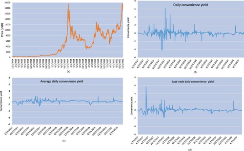
Figure 1(a) is a plot of Bitcoin prices downloaded from Coinbase. Daily observations begin 12/1/2014 and end 12/5/2020. Prices in this period ranged from a low of $370 (less than $0.10 in July of 2010) and during this period the high was $19,948 on 12/4/2020. Prices during this period are best characterized as highly volatile leading an active market for options.

Figure 1. (a) Daily bitcoin closing price from the coinbase exchange. (b) Daily convenience yield implied from put-call-parity. (c) Average daily convenience yield implied from the cost-of-carry model. (d) Daily convenience yield implied from cost-of-carry and last daily trade.

4. Estimating bitcoin convenience yield

Miltersen and Schwartz (1998) develop distribution-free convenience yield estimation methods using the cost-of-carry model. They highlight the difference between the term structure of CY and spot CY and write (14) $J(t,T)=P_t{e}^{{\int }_t^T\left(r\right(t,s)-c(t,s\left)\right)\mathrm{d}s},$(14) where $J(t,T)$ is the price at time-t of a forward contract expiring at T, $r(t,s)$ is the instantaneous continuously compounded futures interest rate and $c(t,s)$ is the continuously compounded term structure of convenience yields. We use $F(t,T)$ $\approx J(t,T)$ to denote futures prices. The approximation is exact when interest rates are independent of the spot and in the special case when interest are constant.

To approximate $c_t$, the spot convenience yield, consider a small increment of time Δ and write (15) $\begin{array}{rl}F(t,t+\mathrm{\Delta })& =S_t{e}^{{\int }_t^{t+\mathrm{\Delta }}\left(r\right(t,s)-c(t,s\left)\right)\mathrm{d}s}\\ & \approx S_t{e}^{\mathrm{\Delta }\left(r\right(t,t)-c(t,t\left)\right)}.\end{array}$(15) Since rates are annualized, spot convenience yield $c(t,t)=c_t$ is approximated as (16) $c_t=r_t-\frac{1}{\mathrm{\Delta }}\ln \left(\frac{F(t,t+\mathrm{\Delta })}{S_t}\right)$(16) for small Δ. In our estimates, we use daily averages, settlement prices, and $\mathrm{\Delta }=15/365$, where the contract matures in 15 days and 365 is the number of trading days in the year. Δ is thus an annualized number as are rates and yields. If the 15-day contract is not available, then we use the next closest maturity.

We use the cost-of-carry model, and put-call parity to estimate CY. See figure 1(b–d). Figure 1(b) is the CY estimate obtained using the dividend form of put-call parity. The sample mean and standard deviation using PCP are 0.0247 and 0.5563, respectively. Figure 1(c) is a plot of daily estimates using the average of each transaction within the day and the cost-of-carry model. The mean and standard deviation of these estimates are 0.0179 and 0.2908. Figure 1(d) is a plot of estimates using the cost-of-carry model and the last transaction of the day. Means and standard deviations were 0.0278 and 0.3913, respectively. It is notable that average CY is positive for all estimates. The CC model with average of transactions within the day is least volatile with a standard deviation of 0.2908. The average estimate of annual CY from the three methods is about 2.35 %.

Our CY estimates differ in sign from those of Ozvatic (2015) and Wu et al. (2021) but are consistent with those of Kim (2021). Ozvatic used the Gibson and Schwartz (1990) commodities model and a regression setup to estimate bitcoin convenience yield from March 3, 2013, until February 18, 2015. He finds a mean (median) convenience yield of $-72.7(-48.3)$, consistent with hacking risks reported during this period. He finds negative but lower CY during the latter part of the period. Wu et al. (2021) used a fractional cointegrated vector autoregressive model and find a negative convenience from December 17, 2018 to July 31, 2021. Kim (2021) finds a positive convenience yield of 5.4 % using the cost-of-carry model and CME tick-by-tick data from December 18, 2017, until December 31, 2019. Our CY estimate is smaller than Kim's. We use different time periods, and data from Deribit while Kim uses data from the CME. Consistent with equation (16(16) $c_t=r_t-\frac{1}{\mathrm{\Delta }}\ln \left(\frac{F(t,t+\mathrm{\Delta })}{S_t}\right)$(16) ), we also use the short-term 15-day futures contract in our calculations.

5. Jump diffusion estimation and pricing results

From our dataset, we construct several subsets to avoid or otherwise account for missing data. Each line in the dataset corresponds to a transaction on either a put or a call. We separate these datasets and augment each by adding CY calculations for each observation. For calls, we define four datasets: Call${}_1$ is the universe of all observations on calls, Call${}_2$ is the subset of observations when there is no missing data for all methods of estimating CY, Call${}_3$ is the subset of observations where there is no missing data when CY is estimated by PCP, Call${}_4$ is the subset of observations when there is no missing data when CY is estimated using the cost-of-carry model. Corresponding datasets are formed for puts.

All data sets and error metrics on in-sample data are used determine the efficacy of different methods of fitting daily option prices. In addition to PCP and CC model estimates, we also imply the daily CY using the JDC model. To do this we use the NLS estimation setup shown in equation (13(13) $L\left({\omega }^{\ast }\right)=\underset{\omega }{min}\sum {\left(C_{\mathrm{m}\mathrm{o}\mathrm{d}\mathrm{e}\mathrm{l}}\right(\omega )-C_{\mathrm{o}\mathrm{b}\mathrm{s}})}^2,$(13) ) and add a constant CY $=c$ to the parameter vector ω. CY error measures are not remarkably different for all four estimation methods. The entire dataset, $Cal{l}_1$ ($Pu{t}_1)$ is available for CY estimates using the JDC model so we chose this model to estimate all eight system parameters plus daily convenience yield.

There were 575,762 observations in the dataset Call${}_1$. To imply daily parameters, we set a daily minimum threshold of 100 observations, leaving a subset set of 564,331 observations. The mean number of observations per day was 433. There were 470,325 observations in the $Pu{t}_1$ dataset. A daily threshold of 100 leaves a subset of 457,123 observations with a mean of 366 daily observations. For each day, we estimated eight parameters plus convenience yield for both datasets and evaluated error metrics for up to 15 days forward.

5.1. Parameter estimates for the jump-diffusion model with convenience yield

Nonlinear Least Squares estimates of parameters and daily convenience yield are given in table 4. The estimates were based on 954 observations on calls and 899 estimates on puts. All parameter estimates are annualized. As noted in the simulations, the optimization surface is relatively flat and individual parameter estimates have wide confidence bands. We note especially the high level and standard deviation of convenience yield volatility estimates, ${\hat{\sigma }}_c$, and this holds for both calls and puts. There is less volatility in estimates of underlying volatility, ${\sigma }_p$. Black–Scholes model estimates of volatility are higher, not surprisingly, since they are implied and must account for other sources of variation such as jumps and convenience yield. As demonstrated in the simulations, pricing estimates are quite accurate, notwithstanding volatility in individual parameters. The operational test of the JDC model is out-of-sample accuracy.

Table 4. NLS parameter estimates.

	Call Estimates (n = 954)		Put Estimates $(n=899)$
Parameter	Mean	Std Dev	Mean	Std Dev
κ	96.4428	113.4389	88.760	108.85
θ	−0.0133	0.6996	−0.3933	1.1319
${\sigma }_p$	0.6242	0.2805	0.5944	0.2969
${\sigma }_c$	13.0763	16.3581	12.962	16.934
ρ	0.1018	0.7327	0.2157	0.7255
λ	5.7484	9.3189	7.4004	9.5714
γ	0.1801	0.5367	−0.1255	0.5669
δ	0.4939	0.7065	0.3607	0.7481
$c_0$	−0.1172	1.2346	0.1254	1.7014

Notes: Nonlinear Least Squares estimates of Jump-Diffusion/Convenience Yield Model annualized parameters. Data covers the period from 1/29/2017 until 6/15/2020. All estimates are for the JD/CY Model except for $c_0,$the average of convenience yields over days. For calls, the estimates of underlying volatility for the Black-Scholes Model, ${\sigma }_{p,}$ was 0.8122 with volatility standard deviation 0.2494. For puts, the corresponding Black-Scholes Model volatility was 0.811with standard deviation 0.2496.

5.2. Pricing estimates

We chose the Absolute Proportional Error (AE) and Proportional Root Mean Square Error (RMSE) as out-of-sample error metrics. The error computations for calls were (17) $\begin{array}{rl}\mathrm{A}\mathrm{E}& =\mathrm{A}\mathrm{v}\mathrm{g}|\hat{C}-C_{\mathrm{o}\mathrm{b}\mathrm{s}}|/\mathrm{A}\mathrm{v}\mathrm{g}\left(C_{\mathrm{o}\mathrm{b}\mathrm{s}}\right),\\ \mathrm{R}\mathrm{M}\mathrm{S}\mathrm{E}& =\left(\sqrt{\sum {(\hat{C}-C_{\mathrm{o}\mathrm{b}\mathrm{s}})}^2/N}\right)/\mathrm{A}\mathrm{v}\mathrm{g}\left(C_{\mathrm{o}\mathrm{b}\mathrm{s}}\right),\end{array}$(17) and similarly for puts. All averages and sums are calculated over daily observations. $\hat{C}$ is the jump diffusion model estimate and $C_{\mathrm{o}\mathrm{b}\mathrm{s}}$ the observed price. Parameter estimates and the set of 15 day out-of-sample estimates are rolled forward each day.

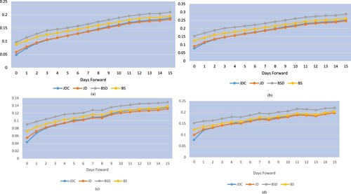
Plots of AE and RMSE metrics for calls and puts are shown in figure 2(a–d). The comparative models were the jump diffusion model with all implied parameters (JDC), the jump-diffusion model without convenience yield (JD), the Black–Scholes model with implied volatility and dividends (BSD) and the Black–Scholes model with implied volatility (BS). The figures show that point estimates of JDC and JD errors are lower than BSD and BS errors for all out-of-sample days forward. Call AE metrics from the JDC (BSD) model are about 7% (11) one day forward and increase monotonically to about 12% (15) five days forward. Put AE metrics are similarly better. The JDC and JD estimates were similar. JDC errors were lower than JD errors in-sample and one day out-of-sample for both metrics. BS metrics are consistently better than BSD metrics in all figures. All errors increase with days out-of-sample and patterns are similar in all figures.

Figure 2. (a) Absolute call errors. (b) RMSE call errors. (c) Absolute put errors. (d) RMSE put errors.

We evaluate the significance of out-of-sample errors using the Diebold and Mariano (1995) statistic. The setup for the AE metric is as follows: the difference in average pricing errors for day-t, normalized by the number of observations, is (18) $d_t=\frac{m_t}{\overline{m}}({\mathrm{A}\mathrm{E}}_{\mathrm{J}\mathrm{D}}-{\mathrm{A}\mathrm{E}}_{\mathrm{B}\mathrm{S}}),t=1,2,\dots ,T,$(18) where T is the number of days in sample, $m_t$ is the number of observations on day-t and $\overline{m}$ is the mean over all days. The same calculations are made for the RMSE metric.

We use a Heteroscedasticity and Autocorrelation Consistent (HAC) estimator to compute standard errors of α in the regression $d_t=\alpha +{ϵ}_t$, $t=1,2,\dots ,T$.³ The null is that $\alpha =0$. The t-statistic on α is the DM test statistic. The DM statistic is computed for JDC versus JD, BSD and BS for puts and calls and both error metrics. Error metrics and DM statics are given in tables 5 and 6 for up to five days out-of-sample.

Table 5. Error metrics and significant tests for calls on BTC.

		Error		DM test statistics
Metric	Days	Avg$|$Error$|$	RMSE	Avg$|$Error$|$	RMSE
Panel A: One day out-of-sample
BS	951	0.1015	0.1430	−6.08***	−5.56***
BSD	951	0.1136	0.1719	−6.99***	−6.56***
JD	951	0.0787	0.1154	−3.75***	−3.04***
JDC	951	0.0736	0.1107
Panel B: Two days out-of-sample
BS	950	0.1156	0.1600	−5.34***	−4.82***
BSD	950	0.1281	0.1882	−6.47***	−5.99***
JD	950	0.0946	0.1341	−2.40**	−1.66*
JDC	950	0.0918	0.1319
Panel C: Three days out-of-sample
BS	949	0.1249	0.1709	−4.54***	−4.16***
BSD	949	0.1403	0.2013	−5.97***	−5.64***
JD	949	0.1054	0.1463	−0.70	−0.37
JDC	949	0.1043	0.1456
Panel D: Four days out-of-sample
BS	948	0.1310	0.1788	−4.20***	−3.76***
BSD	948	0.1454	0.2070	−5.45***	−5.07***
JD	948	0.1129	0.1557	−0.13	0.28
JDC	948	0.1127	0.1562
Panel E: Five days out-of-sample
BS	947	0.1381	0.1885	−4.31***	−3.77***
BSD	947	0.1504	0.2143	−5.19***	−4.76***
JD	847	0.1206	0.1661	0.15	0.94
JDC	947	0.1208	0.1676

Notes: JD denotes jump-diffusion model without convenience yield, JDC denotes jump-diffusion model with convenience yield, BS denotes the Black-Scholes model with implied volatility, and BSD denotes the Black-Scholes model with implied dividends and volatility. Columns 3 and 4 report the mean of daily error metrics: average absolute error (Avg—Error—) and root-mean- square error (RMSE). The last two columns report the Diebold-Mariano test statistics for significant differences between the JDC model versus other models' error metrics. *, ** and *** denote statistical significance at 10%, 5%, and 1% respectively. The data for calls is from December 1, 2016 to June 15, 2020.

Table 6. Error metrics and significant tests for puts on BTC.

		Error		DM test statistics
Metric	Days	Avg$|$Error$|$	RMSE	Avg$|$Error$|$	RMSE
Panel A: One day out-of-sample
BS	898	0.0834	0.1360	-6.38***	-4.70***
BSD	898	0.0976	0.1606	-6.78***	-5.68***
JD	898	0.0722	0.1236	-2.89***	-1.34
JDC	898	0.0672	0.1201
Panel B: Two days out-of-sample
BS	897	0.0914	0.1415	-4.43***	-2.80***
BSD	897	0.1040	0.1632	-6.19***	-5.31***
JD	897	0.0822	0.1313	-1.02	-0.17
JDC	897	0.0803	0.1308
Panel C: Three days out-of-sample
BS	896	0.0973	0.1503	-5.03***	-2.71***
BSD	896	0.1103	0.1716	-6.84***	-5.93***
JD	896	0.0888	0.1410	-1.06	0.15
JDC	896	0.0875	0.1413
Panel D: Four days out-of-sample
BS	895	0.1030	0.1573	-5.03***	-2.41***
BSD	895	0.1169	0.1792	-6.69***	-5.76***
JD	895	0.0942	0.1478	-0.52	0.42
JDC	895	0.0936	0.1490
Panel E: Five days out-of-sample
BS	894	0.1061	0.1586	-1.72*	-0.01
BSD	894	0.1189	0.1787	-4.69***	-2.91***
JD	894	0.0987	0.1506	1.51	1.28
JDC	894	0.1017	0.1585

Notes: JD denotes jump-diffusion model without convenience yield, JDC denotes jump-diffusion model with convenience yield, BS denotes Black-Scholes model with implied volatility, and BSD denotes Black-Scholes model with implied dividends and volatility. Columns 3 and 4 report the mean of daily error metrics: average absolute error (Avg—Error—) and root-mean- square error (RMSE). The last two columns report the Diebold-Mariano test statistics for significant differences between the JDC model versus other models' error metrics. *, ** and *** denote statistical significance at 10%, 5%, and 1% respectively. The data for puts is from November 29, 2016 to June 15, 2020.

Call results are given in table 5. The JDC model AE and RMSE metrics are significantly smaller than BS and BSD for all days forward. The AE metrics for the JDC model are significantly smaller than those of the JD model one and two days forward. The JDC metrics are not significantly different from JD metrics at horizons longer than three days.

The put results given in table 6 are similar to the results for calls. JDC metrics are significantly smaller than BSC and BS metrics at all horizons except the five day horizon. Similarly, the JDC metric is significantly smaller than the JD metric only at one day forward.

6. Summary and conclusions

We investigate convenience yields and option prices for the very volatile and controversial bitcoin cryptocurrency. Using the standard risk neutral valuation setup for equilibrium pricing, we develop a jump-diffusion model with mean-regressive convenience yield. The model has additional parameters but the same form and tractability as the original Merton (1976) model.

Using real data and simulations to validate estimators, we make these notable findings: (1) Bitcoin convenience yields on average are positive and over 2% per year. This contrasts with some earlier studies that find large and negative convenience yields. The differences are likely due to different time periods, different data platforms, and different estimation techniques. However, figure 1(b–d) shows daily yields that can be as small as negative four percent. This is more consistent with a convenience yield (which can be negative) than a currency rate, (2) in simulations, NLS estimates of jump diffusion parameters are unstable, but in net provide accurate estimates of jump diffusion prices with known parameters, and (3) using a large data set spanning most of the years 2016 to 2020, the Merton jump-diffusion model with and without convenience yield significantly outperforms similar versions of the Practitioner Black–Scholes model in out-of-sample tests.

Disclosure statement

No potential conflict of interest was reported by the author(s).

Data availability statement

The data that support the findings of this study were obtained from the following public sources as of July 2020: (a) Deribit's application programming interface (API), retrieved from https://docs.deribit.com/ (b) US Department of the Treasury's website, retrieved from https://home.treasury.gov/policy-issues/financing-the-government/interest-rate-statistics.

Notes

1 Many jumps in crypto prices have coincided with the occurrence of hacks, unsuccessful fork attempts, and government intervention or announcements.

2 We use iterated expectations and further specify that $E[P_t-K{]}^{+}=$ $E_n\left[E_{P_t|n}\right[[P_t-K{]}^{+}]|n]$. Expectations $E_n$ and $E_{P_t|n}$ are taken over the pdf of n and the pdf of $P_t|n$, respectively.

3 We use Newey-West to compute HAC standard errors.

Appendix

Beginning with equation (9(9) $C_n=P_0{e}^{{\mu }_{X|n}+\frac{{\sigma }_{X|n}^2}{2}}N\left(d_1\right)-K{e}^{-rt}N\left(d_2\right),$(9) ) in the text, write the conditional call price as (A1) $C_n=P_0{e}^{{\mu }_{X|n}+\frac{{\sigma }_{X|n}^2}{2}}N\left(d_1\right)-K{e}^{-rt}N\left(d_2\right),$(A1) where N is the standard normal cumulative distribution function and (A2) $\begin{array}{rl}{X}_t& =-(\frac{{\sigma }_p^2}{2}+\lambda \overline{J})t-{\int }_0^{t}c\left(s\right)\mathrm{d}s\\ & +{\sigma }_p{\int }_0^t\mathrm{d}{W}_p+{\sum }_{i=0}^n\ln (1+J_i),‘\\ d_1& =\frac{\ln \left(\frac{P_0}{K}\right)+{\mu }_{X|n}-{\mu }_{Y|n}+{\sigma }_{X|n}^2}{{\sigma }_{X|n}},\\ d_2& =d_1-\sqrt{\mathrm{V}\mathrm{a}\mathrm{r}\left[X|n\right]},\end{array}$(A2) where (A3) $\begin{array}{rl}E[X_t|n=\overline{n}]& :={\mu }_{X|n}\\ & =-(\frac{{\sigma }_s^2}{2}+\lambda \overline{J})t-\frac{(1-e^{-\kappa t})}{\kappa }{c}_0\\ & -\theta (t-\frac{1-e^{-\kappa t}}{\kappa })\\ & +n(\gamma -\frac{{\delta }^2}{2}),\end{array}$(A3) and (A4) $\begin{array}{rl}\mathrm{V}\mathrm{a}\mathrm{r}[X_t|n=\overline{n}]& ={\sigma }_{X|n}^2\\ & ={\sigma }_p^{2}t+{\sigma }_c^2(\frac{t}{{\kappa }^2}+\frac{4e^{-\kappa t}-e^{-2\kappa t}-3}{2{\kappa }^3})\\ & -\frac{2}{\kappa }{\rho }_{pc}{\sigma }_s{\sigma }_c(t-\frac{1-e^{-\kappa t}}{\kappa })+n{\delta }^2,\end{array}$(A4)

since (A5) $\begin{array}{rl}& \mathrm{V}\mathrm{a}\mathrm{r}{\int }_0^t(\frac{e^{\kappa s}-1}{\kappa }-\frac{1}{\kappa }(1-e^{-\kappa t})e^{\kappa s}){\sigma }_c\mathrm{d}{Z}_c\left(s\right)\\ & ={\sigma }_c^2{\int }_0^t{(\frac{e^{\kappa s}-1}{\kappa }-\frac{1}{\kappa }(1-e^{-\kappa t})e^{\kappa s})}^2\mathrm{d}s\left(\mathrm{b}\mathrm{y}\mathrm{I}\mathrm{t}\mathrm{o}\mathrm{I}\mathrm{s}\mathrm{o}\mathrm{m}\mathrm{e}\mathrm{t}\mathrm{r}\mathrm{y}\right)\\ & ={\sigma }_c^2(\frac{t}{{\kappa }^2}+\frac{4e^{-\kappa t}-e^{-2\kappa t}-3}{2{\kappa }^3}),\end{array}$(A5) and (A6) $\begin{array}{rl}& -{\sigma }_p{\sigma }_{c}Cov[{\int }_0^t\mathrm{d}{Z}_p\left(u\right),{\int }_0^t\left(\frac{1}{\kappa }(1-e^{-\kappa v})\right)\mathrm{d}{Z}_c\left(v\right)]\\ & =-{\rho }_{sc}{\sigma }_s{\sigma }_c{\int }_0^t\frac{1}{\kappa }(1-e^{-\kappa u})\mathrm{d}u\\ & =-\frac{1}{\kappa }{\rho }_{sc}{\sigma }_s{\sigma }_c(t-\frac{1-e^{-\kappa t}}{\kappa })\end{array}$(A6) Results for $E[X_t|n=\overline{n}]$ $={\mu }_{X|n}$ and $\mathrm{V}\mathrm{a}\mathrm{r}[X|n=\overline{n}]=$ ${\sigma }_{X|n}^2$ define the conditional option price. The unconditional price for a call is (A7) $C=\sum _{n=0}^{\mathrm{\infty }}{e}^{-\lambda t}\frac{{\left(\lambda t\right)}^n}{n!}{C}_n.$(A7) Conditional put price $\left(H_n\right)$ is given by (A8) $H_n=K{e}^{-rt}N(-d_2)-P_0{e}^{{\mu }_{X|n}+\frac{{\sigma }_{X|n}^2}{2}}N(-d_1).$(A8)

References

- Amin, K.I. and Jarrow, R.A., Pricing foreign currency options under stochastic interest rates. J. Int. Money Finance, 1991, 10(3), 310–329.
- Athey, S., Parashkevov, I., Sarukkai, V. and Xia, J., Bitcoin pricing, adoption, and usage: Theory and evidence. Working paper, Stanford Graduate School of Business, 2016.
- Bakshi, G., Cao, C. and Chen, Z., Empirical performance of alternative option pricing models. J. Finance, 1997, 52(5), 2003–2049.
- Ball, C.A. and Torous, W.N., On jumps in common stock prices and their impact on call option pricing. J. Finance, 1985, 40, 155–173.
- Barth, J.R., Herath, H.S., Herath, T.C. and Xu, P., Cryptocurrency valuation and ethics: A text analytic approach. J. Manag. Anal., 2020, 7(3), 367–388.
- Bates, D.S., The crash of 87: Was it expected? The evidence from options markets. J. Finance, 1991, 46(3), 1009–1044.
- Bates, D.S., Jumps and stochastic volatility: Exchange rate processes implicit in deutsche mark options. Rev. Financ. Stud., 1996, 9(1), 69–107.
- Baur, D.G. and Dimpfl, T., Price discovery in bitcoin spot or futures?. J. Futures Mark., 2019, 39, 803–817.
- Baur, D.G., Hong, K. and Lee, A.D., Bitcoin: Medium of exchange or speculative assets?. J. Int. Financ. Mark. Inst. Money, 2018, 54, 177–189.
- Biais, B., Bisiere, C., Bouvard, M., Casamatta, C. and Menkveld, A.J., Equilibrium bitcoin pricing. Available at SSRN 3261063. 2020.
- Bianchi, D., Cryptocurrencies as an asset class? An empirical assessment. J. Altern. Invest., 2020, 23(2), 162–179.
- Böhme, R., Christin, N., Edelman, B. and Moore, T., Bitcoin: Economics, technology, and governance. J. Econ. Perspect., 2015, 29(2), 213–238.
- Borri, N., Conditional tail-risk in cryptocurrency markets. J. Empir. Finance, 2019, 50, 1–19.
- Bouri, E., Molnár, P., Azzi, G., Roubaud, D. and Hagfors, L.I., On the hedge and safe haven properties of Bitcoin: Is it really more than a diversifier?. Finance Res. Lett., 2017, 20, 192–198.
- Cao, M. and Celik, B., Valuation of Bitcoin options. J. Futures Mark., 2021, 1–20. doi:10.1002/fut.22214
- Chaim, P. and Laurini, M.P., Volatility and return jumps in bitcoin. Econ. Lett., 2018, 173, 158–163.
- Chaim, P. and Laurini, M.P., Is Bitcoin a bubble?. Phys. A Stat. Mech. Appl., 2019, 517, 222–232.
- Cheah, E.T. and Fry, J., Speculative bubbles in Bitcoin markets? An empirical investigation into the fundamental value of Bitcoin. Econ. Lett., 2015, 130, 32–36.
- Cheung, A., Roca, E. and Su, J.J., Crypto-currency bubbles: An application of the Phillips–Shi–Yu (2013) methodology on Mt. Gox bitcoin prices. Appl. Econ., 2015, 47(23), 2348–2358.
- Chiu, J. and Koeppl, T., The economics of cryptocurrency—Bitcoin and beyond. Working Paper, Queen's University, 2017.
- Cong, L.W., Li, Y. and Wang, N., Token-based platform finance. Fisher College of Business Working Paper, (2019-03), p. 028, 2020.
- Corbet, S., Lucey, B. and Yarovaya, L., Datestamping the Bitcoin and Ethereum bubbles. Finance Res. Lett., 2018, 26, 81–88.
- Cretarola, A. and Figà-Talamanca, G., Detecting bubbles in Bitcoin price dynamics via market exuberance. Ann. Oper. Res., 2021, 299(1–2), 459–479.
- Cretarola, A., Figà-Talamanca, G. and Patacca, M., Market attention and Bitcoin price modeling: Theory, estimation and option pricing. Decis. Econ. Finance, 2020, 43(1), 187–228.
- Detzel, A., Liu, H., Strauss, J., Zhou, G. and Zhu, Y., Learning and predictability via technical analysis: Evidence from Bitcoin and stocks with hard-to-value fundamentals. Financ. Manag., 2020, doi:10.1111/fima.12310
- Diebold, F.X. and Mariano, R.S., Comparing predictive accuracy. J. Bus. Econ. Stat., 1995, 13, 252–263.
- Dyhrberg, A.H., Bitcoin, gold and the dollar—A GARCH volatility analysis. Finance Res. Lett., 2016, 16, 85–92.
- Dwyer, G.P., The economics of Bitcoin and similar private digital currencies. J. Financ. Stab., 2015, 17, 81–91.
- Evans, D.S., Economic aspects of Bitcoin and other decentralized public-ledger currency platforms. University of Chicago Coase-Sandor Institute for Law & Economics Research Paper, 685, 2014.
- Foley, S., Karlsen, J.R. and Putniņš, T.J., Sex, drugs, and bitcoin: How much illegal activity is financed through cryptocurrencies?. Rev. Financ. Stud., 2019, 32(5), 1798–1853.
- Gibson, R. and Schwartz, E., Stochastic convenience yield and the pricing of oil contingent claims. J. Finance, 1990, 45(3), 959–976. Papers and Proceedings
- Gronwald, M., Is Bitcoin a commodity? on price jumps, demand shocks, and certainty of supply. J. Int. Money. Finance, 2019, 97, 86–92.
- Hafner, C.M., Testing for bubbles in cryptocurrencies with time-varying volatility. J. Financ. Econom., 2020, 18(2), 233–249.
- He, C., Kennedy, J.S., Coleman, T.F., Forsyth, P.A., Li, Y. and Vetzal, K.R., Calibration and hedging under jump-diffusion. Rev. Deriv. Res., 2006, 9, 1–35.
- Hilliard, J.E. and Hilliard, J., Option pricing under short-lived arbitrage: Theory and tests. Quant. Finance, 2017, 17(11), 1661–1681.
- Hou, A.J., Wang, W., Chen, C.Y. and Härdle, W.K., Pricing cryptocurrency options. J. Financ. Econom., 2020, 18(2), 250–279.
- Jo, H., Park, H. and Shefrin, H., Bitcoin and sentiment. J. Futures Mark., 2020, 40, 1861–1879.
- Jorion, P., On jump processes in the foreign exchange and stock markets. Rev. Financ. Stud., 1988, 1, 427–445.
- Kang, N. and Kim, J., An empirical analysis of Bitcoin price jump risk. Sustainability, 2019, 11(7), 2012.
- Kang, H.J., Lee, S.G. and Park, S.Y, Information efficiency in the cryptocurrency market: The efficient-market hypothesis. J. Comput. Inf. Syst., 2022, 62(3), 622–631.
- Kim, S.T., Is it worth to hold bitcoin?. Finance Res. Lett., 2021, doi:10.1016/j.frl.2021.102090
- Kyriazis, N., Papadamou, S. and Corbet, S, A systematic review of the bubble dynamics of cryptocurrency prices. Res. Int. Bus. Finance, 2020, 54, Article ID 101254.
- Krückeberg, S. and Scholz, P., Decentralized efficiency? Arbitrage in bitcoin markets. Financ. Anal. J., 2020, 76(3), 135–152.
- Krueckeberg, S. and Scholz, P., Cryptocurrencies as an asset class. In Cryptofinance and Mechanisms of Exchange, edited by S. Goutte, K. Guesmi, and S. Saadi, pp. 1–28, 2019 (Springer: Cham).
- Li, L., Arab, A., Liu, J., Liu, J. and Han, Z., Bitcoin options pricing using LSTM-based prediction model and blockchain statistics. In 2019 IEEE International Conference on Blockchain (Blockchain), pp. 67–74. IEEE, 2019a.
- Li, Z.Z., Tao, R., Su, C.W. and Lobonţ, O.R., Does Bitcoin bubble burst?. Qual. Quant., 2019b, 53(1), 91–105.
- Liu, Y. and Tsyvinski, A., Risks and returns of cryptocurrency. Working paper, National Bureau of Economic Research (No. w24877), 2018.
- Makarov, I. and Schoar, A., Trading and arbitrage in cryptocurrency markets. J. Financ. Econ., 2020, 135(2), 293–319.
- Manahov, V. and Urquhart, A., The efficiency of Bitcoin: A strongly typed genetic programming approach to smart electronic Bitcoin markets. Int. Rev. Financ. Anal., 2021, 73, Article ID 101629.
- Merton, R.C., Option pricing when underlying stock returns are discontinuous. J. Financ. Econ., 1976, 3(1–2), 125–144.
- Miltersen, K.R. and Schwartz, E.S., Pricing of options on commodity futures with stochastic term structures of convenience yields and interest rates. J. Financ. Quant. Anal., 1998, 33(1), 33–59.
- Nadarajah, S. and Chu, J., On the inefficiency of Bitcoin. Econ. Lett., 2017, 150, 6–9.
- Ozvatic, S., An analysis of bitcoin spot and futures markets. www.researchonline.mq.edu.au, 2015.
- Pagnottoni, P., Neural network models for Bitcoin option pricing. Front. Artif. Intell., 2019, 2, 5.doi:10.3389/frai.2019.00005
- Philippas, D., Rjiba, H., Guesmi, K. and Goutte, S., Media attention and Bitcoin prices. Finance Res. Lett., 2019, 30, 37–43.
- Pieters, G. and Vivanco, S., Financial regulations and price inconsistencies across Bitcoin markets. Inf. Econ. Policy, 2017, 39, 1–14.
- Raskin, M. and Yermack, D., Digital currencies, decentralized ledgers and the future of central banking. In Research Handbook on Central Banking, edited by P. Conti-Brown, and R.M. Lastra, pp. 474–486, 2018 (Edward Elgar Publishing: Northampton, MA).
- Scaillet, O., Treccani, A. and Trevisan, C., High-frequency jump analysis of the bitcoin market. J. Financ. Econom., 2020, 18(2), 209–232.
- Schilling, L. and Uhlig, H., Some simple bitcoin economics. J. Monet. Econ., 2019, 106, 16–26.
- Shynkevitch, A., Impact of Bitcoin futures on the informational efficiency of the bitcoin spot market. J. Futures Mark., 2020, 41, 115–134.
- Siu, T.K. and Elliott, R.J., Bitcoin option pricing with a SETAR-GARCH model. Eur. J. Finance, 2020, doi:10.1080/1351847X.2020.1828962
- Waters, G.A. and Bui, T., An empirical test for bubbles in cryptocurrency markets. J. Econ. Finance, 2022, 46(1), 207–219.
- Weber, B., Bitcoin and the legitimacy crisis of money. Camb. J. Econ., 2016, 40(1), 17–41.
- Wu, J, Xu, K., Zheng, X. and Chen, J., Fractional cointegration in bitcoin spot and futures markets. J. Futures Mark., 2021, May, doi:10.1002/fut.22216
- Yelowitz, A. and Wilson, M., Characteristics of Bitcoin users: An analysis of Google search data. Appl. Econ. Lett., 2015, 22(13), 1030–1036.
- Yermack, D., Is Bitcoin a real currency? An economic appraisal. In Handbook of Digital Currency, edited by D.K.C. Lee, pp. 31–43, 2015 (Academic Press).
Appendix
Beginning with equation (Equation9(9)
(9) ) in the text, write the conditional call price as
(A1)
where N is the standard normal cumulative distribution function and
(A2)
(A2) where
(A3)
and
(A4)
since
(A5)
(A6)
Results for
define the conditional option price. The unconditional price for a call is
(A7)
Conditional put price