Improving the asymmetric stochastic volatility model with ex-post volatility: the identification of the asymmetry

Abstract

Simulation studies show that the asymmetry stochastic volatility (ASV) models may infer erroneous correlation coefficients, due to their predetermined return-volatility specification. We propose identifying the correlation parameter by incorporating the ex-post volatility in the ASV framework. We obtain a significantly smaller magnitude in the estimated correlation coefficients between equity and volatility processes among major U.S. equity market indexes. Out-of-sample index return distribution forecasts demonstrate superior performance when jointly estimating the return and the ex-post volatility processes. The corrected return-volatility correlations by estimating proposed ASV models with subsample data further document the time-varying leverage effect.

Keywords:

• Asymmetric stochastic volatility
• Leverage effect
• Time-varying asymmetry
• Bayesian MCMC
• Density forecasting
• Realized volatility measures

JEL Classifications:

• C11
• C15
• C22
• C52

1. Introduction

Since the seminal work by Engle (1982), stochastic volatility (SV) has become a key component for financial time series modeling. The asymmetric stochastic volatility (ASV) model, which explicitly identifies the asymmetric correlation between equity returns and their volatility, is an important extension of the simple stochastic volatility (SV) model. In this paper, we discuss the potential misidentification of the return-volatility correlation in the ASV model, as a consequence of modeling the correlation without observing both return and volatility series. We further show that the joint estimation of return and volatility (using realized volatility or bi-power variation) under the ASV framework leads to a more accurate return-volatility correlation estimation, supported by the return density forecasting comparison. Moreover, we show how the corrected estimation of the return-volatility correlation reveals the time-varying asymmetry, which the traditional ASV model misses.

Classical volatility models, such as the GARCH (Bollerslev 1986) model and the SV model (Taylor 2008), and numerous related extensions of such models utilize the standalone return series to infer the stochastic volatility process. Equity returns tend to be negatively correlated with current or future volatility changes. This asymmetry effect is more pronounced for stock market indexes than individual stocks (Kim and Kon 1994, Tauchen et al. 1996, Andersen et al. 2001). Harvey and Shephard (1996) introduce an asymmetric stochastic volatility specification (ASV-HS hereafter), where the equity return innovation is correlated with future volatility changes. Jacquier et al. (2004) propose an alternative asymmetric stochastic volatility specification (ASV-JPR hereafter), in which return innovation is correlated with contemporaneous volatility changes. In comparing these two model specifications, Yu (2005) shows that the return series under the ASV-JPR specification is not a martingale and that ASV-HS is superior to ASV-JPR using a model fitting (marginal likelihood) comparison.

The standard ASV model estimates the correlation coefficient between the equity return, which is observable, and the inferred latent volatility process, which is completely determined by the return series. In this paper, we use simulation studies to show that the standard ASV models tend to produce erroneous estimations of the return-volatility correlation coefficients. The ASV-HS and ASV-JPR models represent asymmetry based on their return-volatility correlation specifications. It is difficult to differentiate the lead-lag or contemporaneous return-volatility correlations by fitting these ASV models with the return series only. In other words, significantly large (with absolute values far from zero and close to one) correlation coefficients from ASV models are insufficient to conclude that the true return-volatility relation is consistent with the corresponding ASV models' specifications. When lead-lag and contemporaneous return-volatility correlations exist in the true model, the ASV-HS model and the ASV-JPR model tend to overestimate the correlation (underestimate the negative correlation coefficient).

The ASV model investigates the return-volatility correlation in the absence of volatility observations, and misidentification is likely to occur. Simulation studies show that incorporating volatility measures, with potential bias and noise, significantly mitigates misidentification when the true volatility process is unobservable. Incorporating an accurate volatility measure enhances the ASV model in accurately identifying the parameters. This improvement diminishes when the volatility measure is noisier. Jointly modeling the return series with a noisy volatility measure has significant misidentification, but the magnitude is smaller.

The potentially erroneous correlation coefficient estimation is misleading when modeling the real-world equity market using standard ASV models. Fitting ASV models with return series alone infer the latent volatility process according to the model's specification and attribute all asymmetric correlations to the model's specification, resulting in an overestimation of the return-volatility correlation (underestimation of the negative correlation coefficient). Inconclusive evidence regarding the causal relationship between equity returns and volatility is found, and the economic interpretation of the asymmetric return-volatility correlation is debatable. We expect to observe both contemporaneous and lead-lag return-volatility correlation with daily data.

Volatility can be measured by the realized volatility measures estimated from high-frequency prices. The realized volatility (RV) and bi-power variation (BV), which are both ex-post variances, are consistent and model-free estimations of the volatility (Andersen and Bollerslev 1998, Barndorff-Nielsen and Shephard 2001, 2004). The RV and BV provide econometricians the support of directly modeling and forecasting the volatility process (Bollerslev et al. 2009, Corsi 2009, Maheu and McCurdy 2011). However, RV or BV is not the true volatility process. It measures the true volatility process biased by microstructure noises (Bandi and Russell 2008, Ait-Sahalia et al. 2011) and non-trading hour bias (Hansen and Lunde 2005, Zhang and Zhao 2020). Previous empirical frameworks (Takahashi et al. 2009, Shirota et al. 2014, Asai et al. 2017, Liu and Maheu 2018) jointly model the return and realized volatility by treating the RV (or logarithmic RV) as an observed series centered around the true volatility (logarithmic volatility) process.

The incorporation of the volatility measures significantly improves the specification and estimation of the ASV models. By jointly modeling the equity return and corresponding volatility measures (see Takahashi et al. 2009), the latent volatility process is no longer endogenously determined by the return series alone. We examine four major U.S. equity indexes ETFs (SPY, DIA, QQQ, and IWM), which are proxies for the S&P 500, the Dow Jones Industrial Average, the NASDAQ 100, and the Russell 2000 indexes, respectively. The sample period ranges from 1998 to 2020, covering two business cycles and supporting our conclusion's robustness. Consistent with the simulation results, the empirical results show that the RV (or BV) measure produces a significantly weaker lead-lag return-volatility correlation, specified as the ASV-HS model.

To support the accuracy of the correlation estimated by jointly modeling return and RV (BV), we show that adding ex-post volatilities significantly improves volatility forecasting from a one-day-ahead return density forecasting perspective. The forecasting comparison supports the accuracy of the lead-lag return-volatility correlation estimated from jointly modeling both return and RV (BV). The predictive superiority is consistent for all four indexes. Combined with the innovation of the ASV framework, the proposed model reflects the predictive relation between current return and future volatility.

The corrected estimation of the lead-lag return-volatility correlation parameter reveals a time-varying leverage effect, which the standard ASV model could omit. Since 2016, the predictive return-volatility correlations have been significantly weaker for major equity indexes. The estimated correlation coefficient could be greater than $-0.2$ for SPY, while the coefficient could be lower than $-0.7$ from 2004 to 2007. Consistent with this Jensen and Maheu (2014), the predictive relationship between return and future volatility depends on the market condition and varies over time. However, the standard ASV-HS model fails to capture the significant differences between the lead-lag return-volatility correlations estimated from different periods of return data (the estimated correlation coefficients range from $-0.8$ to $-0.6$ over time), which is expected as a consequence of the misidentification problem.

Our paper contributes to the extant literature in three aspects. First, we show through simulation analysis that the standard ASV models may have misidentified the correlation structure due to their limited model specification. Second, we propose model improvements to correct this misidentification on correlation estimation by incorporating the ex-post volatility. Lastly, we provide consistent evidence of the time-varying leverage effect, which the standard ASV-HS model misses.

The rest of the paper is organized as follows. Section 2 presents the ASV-HS/ASV-JPR models with their corresponding specifications on the volatility measures. We illustrate in Section 3 how the ASV-HS model generates pseudo-correlation coefficients, and demonstrate how incorporating a volatility measure mitigates this problem. Section 4 discusses the data set covered in this paper. Section 5 presents the empirical results of in-sample estimation and out-of-sample comparisons and shows the time-varying leverage effect. We conclude the paper in Section 7.

2. Model specifications and estimations

2.1. Asymmetric stochastic volatility models

The continuous asymmetric stochastic volatility process of the logarithmic equity price $S_t$ and the corresponding centered logarithmic volatility process $\log \left({\sigma }_t^2\right)$ (see Yu 2005) are: (1) $\begin{array}{rl}\mathrm{d}{S}_t& =\mu \mathrm{d}t+{\sigma }_t{\sigma }_y\mathrm{d}{B}_t^y,\end{array}$(1) (2) $\begin{array}{rl}\mathrm{d}\log \left({\sigma }_t^2\right)& =\text{β}\log \left({\sigma }_t^2\right)\mathrm{d}t+{\sigma }_h\mathrm{d}{B}_t^h.\end{array}$(2) Under our specification, there is no constant term in the volatility process (equation (2(2) $\begin{array}{rl}\mathrm{d}\log \left({\sigma }_t^2\right)& =\text{β}\log \left({\sigma }_t^2\right)\mathrm{d}t+{\sigma }_h\mathrm{d}{B}_t^h.\end{array}$(2) )). However, it is equivalent to having a constant term ${\sigma }_y$ in equation (1(1) $\begin{array}{rl}\mathrm{d}{S}_t& =\mu \mathrm{d}t+{\sigma }_t{\sigma }_y\mathrm{d}{B}_t^y,\end{array}$(1) ) so that the volatility process is a centered volatility process with an unconditional mean of 0. $\mathrm{d}{B}_t^y$ and $\mathrm{d}{B}_t^h$ are two Brownian processes with $B_t^y\mathrm{d}{B}_t^h=\rho \mathrm{d}t$. The consensus on this correlation coefficient is $\rho <0$.

To estimate the discrete-time SV model, we need to discretize this continuous model. We can choose either forward difference ($\mathrm{d}t\approx △t=t+1-t$) or backward difference ($\mathrm{d}t\approx △t=t-t-1$). If we choose backward difference in the price equation (1(1) $\begin{array}{rl}\mathrm{d}{S}_t& =\mu \mathrm{d}t+{\sigma }_t{\sigma }_y\mathrm{d}{B}_t^y,\end{array}$(1) ), i.e., $\mathrm{d}{S}_t\approx S_t-S_{t-1}$ and forward difference in the volatility equation (2(2) $\begin{array}{rl}\mathrm{d}\log \left({\sigma }_t^2\right)& =\text{β}\log \left({\sigma }_t^2\right)\mathrm{d}t+{\sigma }_h\mathrm{d}{B}_t^h.\end{array}$(2) ), i.e., $\mathrm{d}\log \left({\sigma }_t^2\right)\approx \log \left({\sigma }_{t+1}^2\right)-\log \left({\sigma }_t^2\right)$, the resulting discrete stochastic volatility model will be the ASV-HS model of Harvey and Shephard (1996) in equations (3(3) $\begin{array}{rl}{y}_t& \equiv \log \left(S_t\right)-\log \left(S_{t-1}\right)=\mu +\exp \left(h_t/2\right)u_t,\\ h_{t+1}& =\delta h_t+v_{t+1},\end{array}$(3) )–(4(4) $\begin{array}{rl}\left[\begin{array}{c}{u}_t\\ v_{t+1}\end{array}\right]& \sim \mathit{N}(\left[\begin{array}{c}0\\ 0\end{array}\right],\left[\begin{array}{cc}{\sigma }_y^2& {\rho }_{HS}{\sigma }_y{\sigma }_h\\ {\rho }_{HS}{\sigma }_y{\sigma }_h& {\sigma }_h^2\end{array}\right]).\end{array}$(4) ). Current return innovation $u_t$ and future volatility innovation $v_{t+1}$ jointly follow a bivariate normal distribution. (3) $\begin{array}{rl}{y}_t& \equiv \log \left(S_t\right)-\log \left(S_{t-1}\right)=\mu +\exp \left(h_t/2\right)u_t,\\ h_{t+1}& =\delta h_t+v_{t+1},\end{array}$(3) (4) $\begin{array}{rl}\left[\begin{array}{c}{u}_t\\ v_{t+1}\end{array}\right]& \sim \mathit{N}(\left[\begin{array}{c}0\\ 0\end{array}\right],\left[\begin{array}{cc}{\sigma }_y^2& {\rho }_{HS}{\sigma }_y{\sigma }_h\\ {\rho }_{HS}{\sigma }_y{\sigma }_h& {\sigma }_h^2\end{array}\right]).\end{array}$(4) This specification is consistent with the leverage effect interpretation, as we can see from the following uni-variate representation of the ASV-HS model: (5) $\begin{array}{rl}{y}_t& =\mu +\exp \left(h_t/2\right)u_t,u_t\sim N(0,{\sigma }_y^2),\\ h_{t+1}& =\delta h_t+\frac{{\rho }_{HS}{\sigma }_h}{{\sigma }_y}{u}_t+\sqrt{1-{\rho }_{HS}^2}{w}_{t+1},\\ & w_{t+1}\sim N(0,{\sigma }_h^2).\end{array}$(5) In equation (5(5) $\begin{array}{rl}{y}_t& =\mu +\exp \left(h_t/2\right)u_t,u_t\sim N(0,{\sigma }_y^2),\\ h_{t+1}& =\delta h_t+\frac{{\rho }_{HS}{\sigma }_h}{{\sigma }_y}{u}_t+\sqrt{1-{\rho }_{HS}^2}{w}_{t+1},\\ & w_{t+1}\sim N(0,{\sigma }_h^2).\end{array}$(5) ), future volatility $h_{t+1}$ can be treated as a dependent variable with current volatility $h_t$ and return innovation $u_t$ as independent variables. The correlation coefficient (${\rho }_{HS}$) measures the effect of current return innovation on future volatility. The return-volatility correlation structure of the ASV-HS model is a lead-lag relation in which current equity return is associated with future volatility and is consistent with the leverage effect interpretation of the asymmetry.

If we take backward difference on both the price and volatility equations ($\mathrm{d}{S}_t\approx S_t-S_{t-1}$ and $d\log \left({\sigma }_t^2\right)\approx \log \left({\sigma }_t^2\right)-\log \left({\sigma }_{t-1}^2\right)$ for (1(1) $\begin{array}{rl}\mathrm{d}{S}_t& =\mu \mathrm{d}t+{\sigma }_t{\sigma }_y\mathrm{d}{B}_t^y,\end{array}$(1) ) and (2(2) $\begin{array}{rl}\mathrm{d}\log \left({\sigma }_t^2\right)& =\text{β}\log \left({\sigma }_t^2\right)\mathrm{d}t+{\sigma }_h\mathrm{d}{B}_t^h.\end{array}$(2) )), the resulting discrete stochastic volatility model will be the ASV-JPR model of Jacquier et al. (2004) in equations (6(6) $\begin{array}{rl}{y}_t& \equiv \log \left(S_t\right)-\log \left(S_{t-1}\right)=\mu +\exp \left(h_t/2\right)u_t,\\ h_t& =\delta h_{t-1}+v_t,\end{array}$(6) )–(7(7) $\begin{array}{rl}\left[\begin{array}{c}{u}_t\\ v_t\end{array}\right]& \sim \mathit{N}(\left[\begin{array}{c}0\\ 0\end{array}\right],\left[\begin{array}{cc}{\sigma }_y^2& {\rho }_{JPR}{\sigma }_y{\sigma }_h\\ {\rho }_{JPR}{\sigma }_y{\sigma }_h& {\sigma }_h^2\end{array}\right]).\end{array}$(7) ). contemporaneous return innovation $u_t$ and volatility innovation $v_t$ jointly follow a bi-variate normal distribution. (6) $\begin{array}{rl}{y}_t& \equiv \log \left(S_t\right)-\log \left(S_{t-1}\right)=\mu +\exp \left(h_t/2\right)u_t,\\ h_t& =\delta h_{t-1}+v_t,\end{array}$(6) (7) $\begin{array}{rl}\left[\begin{array}{c}{u}_t\\ v_t\end{array}\right]& \sim \mathit{N}(\left[\begin{array}{c}0\\ 0\end{array}\right],\left[\begin{array}{cc}{\sigma }_y^2& {\rho }_{JPR}{\sigma }_y{\sigma }_h\\ {\rho }_{JPR}{\sigma }_y{\sigma }_h& {\sigma }_h^2\end{array}\right]).\end{array}$(7) Similarly, the following uni-variate representation of the ASV-JPR model shows no lead-lag relation between return and volatility. (8) $\begin{array}{rl}{y}_t& =\mu +\exp \left(h_t/2\right)u_t,u_t\sim N(0,{\sigma }_y^2),\\ h_t& =\delta h_{t-1}+\frac{{\rho }_{JPR}{\sigma }_h}{{\sigma }_y}{u}_t+\sqrt{1-{\rho }_{JPR}^2}{w}_t,w_t\sim N(0,{\sigma }_h^2).\end{array}$(8) Given equation (8(8) $\begin{array}{rl}{y}_t& =\mu +\exp \left(h_t/2\right)u_t,u_t\sim N(0,{\sigma }_y^2),\\ h_t& =\delta h_{t-1}+\frac{{\rho }_{JPR}{\sigma }_h}{{\sigma }_y}{u}_t+\sqrt{1-{\rho }_{JPR}^2}{w}_t,w_t\sim N(0,{\sigma }_h^2).\end{array}$(8) ), we cannot identify either volatility feedback or the leverage effect (Men et al. 2017) as this model's return and volatility innovations are immediate. The return-volatility correlation structure of the ASV-JPR model is consistent with the contemporaneous asymmetric correlation, especially at lower frequencies, like weekly or even monthly, where we cannot differentiate between return and volatility in the lead-lag relation.

For comparison purposes, we also estimate the following symmetric stochastic volatility model (SV model), in which the return and latent volatility innovations are not correlated, in the empirical result section (Section 5): $\begin{array}{rl}{y}_t& =\mu +\exp \left(h_t/2\right)u_t,u_t\sim N(0,{\sigma }_y^2),\\ h_t& =\delta h_{t-1}+w_t,w_t\sim N(0,{\sigma }_h^2).\end{array}$ If we have a volatility measure denoted as $V{M}_t$, we can jointly model the return $y_t$ and the volatility measure $V{M}_t$ (see Takahashi et al. 2009). Combining the ASV-HS model with a volatility measure leads to the following VMASV-HS model specification: (9) $\begin{array}{rl}{y}_t& =\mu +\exp \left(h_t/2\right)u_t,\\ h_{t+1}& =\delta h_t+v_{t+1},\\ V{M}_t& =\xi +h_t+e_t,e_t\sim N(0,{\sigma }_{VM}^2),\\ \left[\begin{array}{c}{u}_t\\ v_{t+1}\end{array}\right]& \sim \mathit{N}(\left[\begin{array}{c}0\\ 0\end{array}\right],\left[\begin{array}{cc}{\sigma }_y^2& {\rho }_{HS}{\sigma }_y{\sigma }_h\\ {\rho }_{HS}{\sigma }_y{\sigma }_h& {\sigma }_h^2\end{array}\right]).\end{array}$(9) Similarly, we could also extend the ASV-JPR model with a volatility measure as the following VMASV-JPR model: (10) $\begin{array}{rl}{y}_t& =\mu +\exp \left(h_t/2\right)u_t,\\ h_t& =\delta h_{t-1}+v_t,\\ V{M}_t& =\xi +h_t+e_t,e_t\sim N(0,{\sigma }_{VM}^2),\\ \left[\begin{array}{c}{u}_t\\ v_t\end{array}\right]& \sim \mathit{N}(\left[\begin{array}{c}0\\ 0\end{array}\right],\left[\begin{array}{cc}{\sigma }_y^2& {\rho }_{JPR}{\sigma }_y{\sigma }_h\\ {\rho }_{JPR}{\sigma }_y{\sigma }_h& {\sigma }_h^2\end{array}\right]).\end{array}$(10) Under this framework, $y_t$ and $V{M}_t$ are jointly modeled with a single volatility factor $h_t$ in the state space model framework. Unlike the ASV model without the volatility measure, $V{M}_t$ will substantially influence the identification of $h_t$ if $V{M}_t$ is an accurate volatility measure. More importantly, the identification of $h_t$ will not depend on $y_t$ alone. Incremental information in $V{M}_t$ will improve the identification of the true volatility process and help clarify the asymmetric relation between return and volatility.

The specification of equations (9(9) $\begin{array}{rl}{y}_t& =\mu +\exp \left(h_t/2\right)u_t,\\ h_{t+1}& =\delta h_t+v_{t+1},\\ V{M}_t& =\xi +h_t+e_t,e_t\sim N(0,{\sigma }_{VM}^2),\\ \left[\begin{array}{c}{u}_t\\ v_{t+1}\end{array}\right]& \sim \mathit{N}(\left[\begin{array}{c}0\\ 0\end{array}\right],\left[\begin{array}{cc}{\sigma }_y^2& {\rho }_{HS}{\sigma }_y{\sigma }_h\\ {\rho }_{HS}{\sigma }_y{\sigma }_h& {\sigma }_h^2\end{array}\right]).\end{array}$(9) ) and (10(10) $\begin{array}{rl}{y}_t& =\mu +\exp \left(h_t/2\right)u_t,\\ h_t& =\delta h_{t-1}+v_t,\\ V{M}_t& =\xi +h_t+e_t,e_t\sim N(0,{\sigma }_{VM}^2),\\ \left[\begin{array}{c}{u}_t\\ v_t\end{array}\right]& \sim \mathit{N}(\left[\begin{array}{c}0\\ 0\end{array}\right],\left[\begin{array}{cc}{\sigma }_y^2& {\rho }_{JPR}{\sigma }_y{\sigma }_h\\ {\rho }_{JPR}{\sigma }_y{\sigma }_h& {\sigma }_h^2\end{array}\right]).\end{array}$(10) ) follows the broad literature on jointly modeling return and realized volatility measures (Takahashi et al. 2009, Koopman and Scharth 2013, Shirota et al. 2014, Venter and De Jongh 2014, Asai et al. 2017).¹ The constant term ξ captures the shift required to adjust $V{M}_t$ so make $V{M}_t-\xi$ an unbiased estimation of the daily logarithmic volatility $E(V{M}_t-\xi |h_t)=h_t$. And the error term $e_t\sim N(0,{\sigma }_{VM}^2)$ is the i.i.d noise of $V{M}_t$. A smaller ${\sigma }_{VM}$ indicates a more accurate volatility measure.

Similarly, we also estimated the symmetric SV model (VMSV) with the volatility measure as follows: $\begin{array}{rl}{y}_t& =\mu +\exp \left(h_t/2\right)u_t,u_t\sim N(0,{\sigma }_y^2),\\ h_t& =\delta h_{t-1}+w_t,w_t\sim N(0,{\sigma }_h^2),\\ V{M}_t& =\xi +h_t+e_t,e_t\sim N(0,{\sigma }_{VM}^2).\end{array}$ The VMSV model will be used as a benchmark model to examine whether modeling the asymmetry is necessary.

2.2. Model estimation

We use Bayesian MCMC for model estimations. The key is to sample the latent volatility $h_t$ since the ASV model can be treated as a simple linear model given $h_t$. We use the Metropolis-Hasting algorithm with tailored proposal distributions. Let $\mathit{h}$ ($\mathit{y}$ and $\mathit{V}\mathit{M}$) denote the latent volatility series $\{h_t{\}}_{t=1}^T$ (the return series $\{y_t{\}}_{t=1}^T$ and the volatility measure series $\{V{M}_t{\}}_{t=1}^T$ ), ${\mathit{h}}_{-t}$ denote the latent volatility series excluding $h_t$ and $\mathbf{\Sigma }$ denote the covariance matrix $\left[\begin{array}{cc}{\sigma }_y^2& \rho {\sigma }_y{\sigma }_h\\ \rho {\sigma }_y{\sigma }_h& {\sigma }_h^2\end{array}\right]$. Denote the set of the parameters $\{\delta ,\mathbf{\Sigma },\xi ,{\sigma }_{VM}\}$ as Θ. We provide details about MCMC estimations in Appendix Section A1. We report the MCMC steps and prior choices as follows:

• $\mathit{h}|\mathit{y},\mathit{V}\mathit{M},\mu ,\delta ,\xi ,{\sigma }_{VM}$: Single-move sampler for $h_t$, $t=1,2\dots T$ with the Metropolis-Hastings algorithm. For the ASV-HS and ASV-JPR models, which do not have the volatility measure, the posterior distributions of $\mathit{h}$ only depend on $\mathit{y}$.

• $\mu ,\delta |\mathit{y},\mathit{h},\mathbf{\Sigma }$: Conjugate normal distribution $N(0,5)$ for μ and truncated normal distribution $N(0.95,5)I_{|\delta |<1}$ for δ for stationarity.

• $\mathbf{\Sigma }|\mathit{y},\mathit{h},\mu ,\delta$: Conjugate Wishart distribution $W(n,S_0^{-1})$, where n = 3 and $S_0=\left[\begin{array}{cc}{0.8}^2& 0\\ 0& {0.3}^2\end{array}\right]$. We set zero correlation in the inverse of the scale matrix. The choices of the degree of freedom guarantee the Wishart prior is uninformative.

• $\xi |\mathit{V}\mathit{M},\mathit{h},{\sigma }_{VM}$: Conjugate normal distribution $N(\overline{VM},5)$. $\overline{VM}$ is the simple average of $V{M}_t$. Since the unconditional mean of $h_t$ is zero, the constant term ξ should be close to $\overline{VM}$. This step is specific to the VMASV-HS and VMASV-JPR models.

• ${\sigma }_{VM}|\mathit{V}\mathit{M},\mathit{h},\xi$: Conjugate inverse gamma prior distribution $IG(\frac{3}{2},\frac{0.5}{2})$. This step is specific to the VMASV-HS and VMASV-JPR models.

We set flat prior distributions for all parameters to avoid subjective bias. Also, we set the total number of MCMC iterations to 100 000 and keep 1 of every 10 draws. We also set 1000 burn-in iterations for parameter convergence.

3. Simulation study of ASV models

3.1. The misidentification of return-volatility correlation

The general data generating process (DGP) for returns ($y_t$) and true volatilities ($h_t$) is specified as follows: (11) $\begin{array}{rl}{y}_t& =\mu +\exp \left(h_t/2\right)u_t,u_t\sim N(0,{\sigma }_y^2),\end{array}$(11) (12) $\begin{array}{rl}{h}_t& =\delta h_{t-1}+\frac{{\rho }_{JPR}{\sigma }_h}{{\sigma }_y}{u}_t+\frac{{\rho }_{HS}{\sigma }_h}{{\sigma }_y}{u}_{t-1}+\sqrt{1-{\rho }_{HS}^2-{\rho }_{JPR}^2}{w}_t,\\ & w_t\sim N(0,{\sigma }_h^2).\end{array}$(12) Where the volatility innovation $v_t\equiv h_t-\delta h_{t-1}$ is correlated with the contemporaneous and lagged return innovations ($u_t$ and $u_{t-1}$) as the following: (13) $\left[\begin{array}{c}{u}_{t-1}\\ u_t\\ v_t\end{array}\right]\sim \mathit{N}(\left[\begin{array}{c}0\\ 0\\ 0\end{array}\right],\left[\begin{array}{ccc}{\sigma }_y^2& 0& {\rho }_{HS}{\sigma }_y{\sigma }_h\\ 0& {\sigma }_y^2& {\rho }_{JPR}{\sigma }_y{\sigma }_h\\ {\rho }_{HS}{\sigma }_y{\sigma }_h& {\rho }_{JPR}{\sigma }_y{\sigma }_h& {\sigma }_h^2\end{array}\right]).$(13) As shown in equation (13(13) $\left[\begin{array}{c}{u}_{t-1}\\ u_t\\ v_t\end{array}\right]\sim \mathit{N}(\left[\begin{array}{c}0\\ 0\\ 0\end{array}\right],\left[\begin{array}{ccc}{\sigma }_y^2& 0& {\rho }_{HS}{\sigma }_y{\sigma }_h\\ 0& {\sigma }_y^2& {\rho }_{JPR}{\sigma }_y{\sigma }_h\\ {\rho }_{HS}{\sigma }_y{\sigma }_h& {\rho }_{JPR}{\sigma }_y{\sigma }_h& {\sigma }_h^2\end{array}\right]).$(13) ), the correlation coefficient ${\rho }_{JPR}$ and ${\rho }_{HS}$ represent the contemporaneous and lead-lag return-volatility correlations respectively. Restricting ${\rho }_{JPR}=0$ (${\rho }_{HS}=0$), equations (11(11) $\begin{array}{rl}{y}_t& =\mu +\exp \left(h_t/2\right)u_t,u_t\sim N(0,{\sigma }_y^2),\end{array}$(11) ) and (12(12) $\begin{array}{rl}{h}_t& =\delta h_{t-1}+\frac{{\rho }_{JPR}{\sigma }_h}{{\sigma }_y}{u}_t+\frac{{\rho }_{HS}{\sigma }_h}{{\sigma }_y}{u}_{t-1}+\sqrt{1-{\rho }_{HS}^2-{\rho }_{JPR}^2}{w}_t,\\ & w_t\sim N(0,{\sigma }_h^2).\end{array}$(12) ) will degenerate into the ASV-HS (ASV-JPR) model and restricting ${\rho }_{JPR}={\rho }_{HS}=0$ leads to the symmetric SV model.

We set the return-volatility correlation (${\rho }_{HS}$ and ${\rho }_{JPR}$) to represent the following three scenarios.²

1. Only the lead-lag return-volatility correlation exists. We let ${\rho }_{HS}$ equal to $-0.2$, $-0.5$ or $-0.8$, while ${\rho }_{JPR}$ equal to 0. The volatility innovation is weakly, moderately, or strongly related to lagged return innovations, but not current return innovation.

2. Only the contemporaneous return-volatility correlation exists. We let ${\rho }_{JPR}$ equal to $-0.2$, $-0.5$ or $-0.8$, while ${\rho }_{HS}$ equal to 0. The volatility innovation is weakly, moderately, or strongly related to current return innovations, but not to lagged return innovation.

3. Both lead-lag and contemporaneous return-volatility correlations exist. First, we let both ${\rho }_{HS}$ and ${\rho }_{JPE}$ equal $-0.2$ (or $-0.5$), indicating that the volatility innovation is weak (or moderately) related to both current and lagged return innovations. We also let ${\rho }_{HS}$ equal to $-0.8$ and ${\rho }_{JPR}$ equal to $-0.2$ (or ${\rho }_{HS}$ equal to $-0.2$ and ${\rho }_{JPR}$ equal to $-0.8$), indicating that the volatility innovation is strongly related to lagged return innovation while weakly related to current return innovation (weakly related to lagged return innovation while strongly related to current return innovation).

We set the remaining parameters ($\mu =0.1$, $\delta =0.96$, ${\sigma }_y=0.9$, ${\sigma }_h=0.3$) according to the estimation results of fitting the symmetric SV model with S&P500 returns, as shown in table 6, which are consistent with previous researches that modeling equity index returns with the SV models. We simulated 200 samples of return and volatility series for each parameter setting, and each sample contained 4000 observations.

To summarize the simulation study's MCMC estimation results, we report the estimated posterior mean, standard deviation, and 95% density intervals across the simulated samples. In addition, we also report the posterior cumulative distribution function at the parameter true value ($F\left(True\right)$), which is the posterior probability of a parameter (θ) smaller than its true value ($P(\theta <True)$). A value of $F\left(True\right)$ close to 1 (or 0) suggest that the model tends to underestimate (overestimate) the parameter.

Table 1 (table 2) shows the estimation results of the ASV-HS and ASV-JPR models in Panel A and B, when there is a lead-lag (contemporaneous) return-volatility correlation specified as the ASV-HS (ASV-JPR) model.

Table 1. Estimation results of fitting ASV-HS and ASV-JPR models with simulated returns: Only lead-lag return-volatility correlation exists.

	${\rho }_{HS}=-0.2$, ${\rho }_{JPR}=0$					${\rho }_{HS}=-0.5$, ${\rho }_{JPR}=0$					${\rho }_{HS}=-0.8$, ${\rho }_{JPR}=0$
	True	Mean	Std	95% D.I.	$F\left(True\right)$	True	Mean	Std	95% D.I.	$F\left(True\right)$	True	Mean	Std	95% D.I.	$F\left(True\right)$
Panel A: ASV-HS
μ	0.1	0.101	0.012	0.078, 0.125	0.463	0.1	0.099	0.012	0.076, 0.123	0.514	0.1	0.103	0.011	0.081, 0.125	0.409
		(0.014)	(0.001)	(0.014), (0.014)	(0.309)		(0.012)	(0.001)	(0.012), (0.011)	(0.295)		(0.011)	(0.001)	(0.012), (0.010)	(0.273)
δ	0.96	0.961	0.006	0.948, 0.972	0.450	0.96	0.960	0.006	0.949, 0.971	0.456	0.96	0.960	0.004	0.951, 0.969	0.467
		(0.006)	(0.001)	(0.008), (0.005)	(0.287)		(0.005)	(0.001)	(0.006), (0.004)	(0.276)		(0.004)	(0.001)	(0.005), (0.004)	(0.293)
${\sigma }_y$	0.9	0.890	0.054	0.787, 1.000	0.574	0.9	0.893	0.053	0.791, 1.001	0.543	0.9	0.886	0.048	0.793, 0.981	0.575
		(0.046)	(0.007)	(0.042), (0.054)	(0.258)		(0.051)	(0.007)	(0.047), (0.057)	(0.292)		(0.046)	(0.005)	(0.044), (0.049)	(0.284)
${\sigma }_h$	0.3	0.297	0.019	0.261, 0.335	0.552	0.3	0.299	0.017	0.266, 0.335	0.534	0.3	0.296	0.014	0.269, 0.326	0.585
		(0.020)	(0.001)	(0.018), (0.021)	(0.301)		(0.016)	(0.001)	(0.015), (0.018)	(0.280)		(0.015)	(0.001)	(0.014), (0.016)	(0.283)
${\rho }_{HS}$	−0.2	−0.201	0.051	−0.299, −0.101	0.490	−0.5	−0.511	0.042	−0.59, −0.426	0.591	−0.8	−0.800	0.025	−0.845, −0.749	0.517
		(0.050)	(0.002)	(0.049), (0.052)	(0.274)		(0.040)	(0.002)	(0.037), (0.042)	(0.262)		(0.025)	(0.002)	(0.021), (0.029)	(0.290)
Panel B: ASV-JPR
μ	0.1	0.113	0.012	0.090, 0.136	0.233	0.1	0.129	0.012	0.106, 0.153	0.031	0.1	0.155	0.012	0.132, 0.177	0.000
		(0.013)	(0.001)	(0.014), (0.013)	(0.250)		(0.011)	(0.001)	(0.011), (0.010)	(0.060)		(0.009)	(0.001)	(0.009), (0.009)	(0.001)
δ	0.96	0.962	0.006	0.949, 0.973	0.403	0.96	0.965	0.006	0.954, 0.976	0.218	0.96	0.974	0.004	0.965, 0.982	0.016
		(0.006)	(0.001)	(0.008), (0.005)	(0.280)		(0.005)	(0.001)	(0.007), (0.004)	(0.221)		(0.004)	(0.001)	(0.005), (0.003)	(0.057)
${\sigma }_y$	0.9	0.891	0.054	0.789, 1.002	0.570	0.9	0.902	0.057	0.795, 1.021	0.497	0.9	0.908	0.064	0.786, 1.038	0.466
		(0.046)	(0.007)	(0.043), (0.053)	(0.258)		(0.0520)	(0.008)	(0.048), (0.060)	(0.283)		(0.0490)	(0.009)	(0.049), (0.060)	(0.249)
${\sigma }_h$	0.3	0.293	0.019	0.258, 0.332	0.601	0.3	0.279	0.018	0.247, 0.316	0.809	0.3	0.247	0.014	0.221, 0.275	0.991
		(0.019)	(0.001)	(0.018), (0.021)	(0.291)		(0.017)	(0.001)	(0.016), (0.020)	(0.216)		(0.014)	(0.001)	(0.013), (0.016)	(0.035)
${\rho }_{JPR}$	0.0	−0.113	0.048	−0.207, −0.019	0.959	0.0	−0.302	0.050	−0.397, −0.203	1.000	0.0	−0.574	0.047	−0.661, −0.478	1.000
		(0.046)	(0.002)	(0.046), (0.046)	(0.070)		(0.046)	(0.002)	(0.045), (0.045)	(0.000)		(0.048)	(0.003)	(0.044), (0.052)	(0.000)

Note: This table summarizes the estimation results of fitting the ASV-HS (panel A) and the ASV-JPR (panel B) models with returns ($y_t$) simulated from the following model: $\begin{array}{rl}{y}_t& =\mu +\exp \left(h_t/2\right)u_t,u_t\sim N(0,{\sigma }_y^2),\\ h_t& =\delta h_{t-1}+\frac{{\rho }_{JPR}{\sigma }_h}{{\sigma }_y}{u}_t+\frac{{\rho }_{HS}{\sigma }_h}{{\sigma }_y}{u}_{t-1}+\sqrt{1-{\rho }_{HS}^2-{\rho }_{JPR}^2}{w}_t,w_t\sim N(0,{\sigma }_h^2),\end{array}$ where $\mu =0.1$, $\delta =0.96$, ${\sigma }_y=0.9$, ${\sigma }_h=0.3$, ${\rho }_{JPR}=0$, and ${\rho }_{HS}=-0.2,-0.5,-0.8$ respectively (the true values are reported in column True for comparison purposes). We simulate 200 samples of 4000 observations. We report the means of MCMC posterior mean (column Mean), standard deviation (column Std), 95% density interval (column 95% D.I), and cumulative distribution at the true value (column $F\left(True\right)$). The corresponding standard deviations across simulated samples are reported in brackets.

Table 2. Estimation results of fitting ASV-HS and ASV-JPR models with simulated returns: Only contemporaneous return-volatility correlation exists.

	${\rho }_{HS}=0$, ${\rho }_{JPR}=-0.2$					${\rho }_{HS}=0$, ${\rho }_{JPR}=-0.5$					${\rho }_{HS}=0$, ${\rho }_{JPR}=-0.8$
	True	Mean	Std	95% D.I.	$F\left(True\right)$	True	Mean	Std	95% D.I.	$F\left(True\right)$	True	Mean	Std	95% D.I.	$F\left(True\right)$
Panel A: ASV-HS
μ	0.1	0.092	0.012	0.068, 0.116	0.673	0.1	0.080	0.012	0.056, 0.104	0.882	0.1	0.064	0.012	0.040, 0.087	0.990
		(0.013)	(0.001)	(0.013), (0.013)	(0.266)		(0.012)	(0.001)	(0.013), (0.012)	(0.140)		(0.011)	(0.001)	(0.013), (0.010)	(0.025)
δ	0.96	0.958	0.006	0.945, 0.970	0.527	0.96	0.955	0.006	0.942, 0.967	0.702	0.96	0.950	0.005	0.939, 0.960	0.917
		(0.007)	(0.001)	(0.009), (0.006)	(0.299)		(0.006)	(0.001)	(0.008), (0.005)	(0.253)		(0.005)	(0.001)	(0.006), (0.004)	(0.126)
${\sigma }_y$	0.9	0.892	0.051	0.796, 0.994	0.566	0.9	0.868	0.045	0.781, 0.958	0.696	0.9	0.837	0.038	0.763, 0.912	0.873
		(0.049)	(0.007)	(0.046), (0.056)	(0.286)		(0.046)	(0.005)	(0.042), (0.052)	(0.262)		(0.040)	(0.004)	(0.039), (0.043)	(0.163)
${\sigma }_h$	0.3	0.300	0.019	0.265, 0.337	0.526	0.3	0.296	0.018	0.263, 0.332	0.583	0.3	0.288	0.015	0.260, 0.320	0.699
		(0.017)	(0.001)	(0.015), (0.019)	(0.274)		(0.018)	(0.001)	(0.015), (0.019)	(0.279)		(0.017)	(0.001)	(0.015), (0.019)	(0.269)
${\rho }_{HS}$	0.0	−0.134	0.051	−0.233, −0.033	0.964	0.0	−0.349	0.049	−0.443, −0.250	1.000	0.0	−0.627	0.043	−0.706, −0.538	1.000
		(0.053)	(0.002)	(0.052), (0.054)	(0.079)		(0.050)	(0.002)	(0.047), (0.052)	(0.000)		(0.045)	(0.003)	(0.040), (0.051)	(0.000)
Panel B: ASV-JPR
μ	0.1	0.099	0.012	0.076, 0.123	0.505	0.1	0.100	0.012	0.077, 0.122	0.49	0.1	0.102	0.011	0.081, 0.124	0.430
		(0.012)	(0.001)	(0.013), (0.012)	(0.284)		(0.011)	(0.001)	(0.012), (0.011)	(0.279)		(0.009)	(0.001)	(0.010), (0.009)	(0.255)
δ	0.96	0.959	0.006	0.946, 0.971	0.478	0.96	0.959	0.006	0.948, 0.970	0.498	0.96	0.960	0.004	0.952, 0.968	0.481
		(0.007)	(0.001)	(0.009), (0.006)	(0.301)		(0.006)	(0.001)	(0.007), (0.005)	(0.288)		(0.004)	(0.000)	(0.004), (0.003)	(0.270)
${\sigma }_y$	0.9	0.892	0.054	0.791, 1.003	0.559	0.9	0.889	0.051	0.791, 0.993	0.57	0.9	0.889	0.048	0.797, 0.984	0.572
		(0.051)	(0.008)	(0.048), (0.057)	(0.283)		(0.050)	(0.007)	(0.048), (0.057)	(0.285)		(0.040)	(0.005)	(0.037), (0.046)	(0.262)
${\sigma }_h$	0.3	0.299	0.019	0.263, 0.337	0.540	0.3	0.298	0.017	0.265, 0.333	0.553	0.3	0.299	0.014	0.273, 0.326	0.531
		(0.018)	(0.002)	(0.017), (0.021)	(0.278)		(0.017)	(0.001)	(0.016), (0.019)	(0.296)		(0.014)	(0.001)	(0.014), (0.015)	(0.298)
${\rho }_{JPR}$	−0.2	−0.201	0.046	−0.290, −0.109	0.506	−0.5	−0.499	0.040	−0.574, −0.419	0.505	−0.8	−0.802	0.023	−0.844, −0.754	0.541
		(0.045)	(0.002)	(0.044), (0.046)	(0.290)		(0.037)	(0.002)	(0.035), (0.040)	(0.290)		(0.022)	(0.002)	(0.019), (0.026)	(0.286)

Note: This table summarizes the estimation results of fitting the ASV-HS (panel A) and the ASV-JPR (panel B) models with returns ($y_t$) simulated from the following model: $\begin{array}{rl}{y}_t& =\mu +\exp \left(h_t/2\right)u_t,u_t\sim N(0,{\sigma }_y^2),\\ h_t& =\delta h_{t-1}+\frac{{\rho }_{JPR}{\sigma }_h}{{\sigma }_y}{u}_t+\frac{{\rho }_{HS}{\sigma }_h}{{\sigma }_y}{u}_{t-1}+\sqrt{1-{\rho }_{HS}^2-{\rho }_{JPR}^2}{w}_t,w_t\sim N(0,{\sigma }_h^2),\end{array}$ where $\mu =0.1$, $\delta =0.96$, ${\sigma }_y=0.9$, ${\sigma }_h=0.3$, ${\rho }_{HS}=0$, and ${\rho }_{JPR}=-0.2,-0.5,-0.8$ respectively (the true values are reported in column True for comparison purposes). We simulate 200 samples of 4000 observations. We report the means of MCMC posterior mean (column Mean), standard deviation (column Std), 95% density interval (column 95% D.I), and cumulative distribution at the true value (column $F\left(True\right)$). The corresponding standard deviations across simulated samples are reported in brackets.

First, we confirm the validity of our estimation method by correctly identifying the true parameter if the return is simulated accordingly (Panel A of table 1 and Panel B of table 2). Moreover, if the SV model generates the return series, both ASV-HS and ASV-JPR models report correlation coefficients close to zero, as shown in table A1 of the Online Appendix.

However, as shown in Panel B of table 1 if only lead-lag return-volatility correlation exists, the ASV-JPR model consistently produces ${\rho }_{JPR}$ that is significantly smaller than zero. When there is weak (${\rho }_{HS}=-0.2$), moderate (${\rho }_{HS}=-0.5$), or strong (${\rho }_{HS}=-0.8$) lead-lag correlation, the ASV-JPR model erroneously estimate ${\rho }_{JPR}=-0.113$, $-0.302$, or $-0.574$ on average.³ Moreover, the posterior probability of ${\rho }_{JPR}<0$ is consistent close to one across simulated samples, as shown by column $F\left(True\right)$ in Panel B of table 1. Similarly, as shown in Panel A of table 2, When it is weak (${\rho }_{JPR}=-0.2$), moderate (${\rho }_{JPR}=-0.5$), or strong (${\rho }_{JPR}=-0.8$) contemporaneous correlation, the ASV-HS model erroneously estimates ${\rho }_{HS}=-0.134$, $-0.349$, or $-0.627$ on average and the posterior probability of ${\rho }_{HS}<0$ is close one across samples. The misidentification is statistically and economically significant for both ASV-HS and ASV-JPR models. An estimated ${\rho }_{HS}$ (${\rho }_{JPR}$) that far from zero of the ASV-HS (ASV-JPR) model does not necessarily support the lead-lag (contemporaneous) return-volatility correlation.⁴

Both ASV models are consistent with the well-documented negative correlation between return and volatility. However, when there is asymmetry, both ASV models can only reflect the asymmetry according to their correlation structure, even though the true structure is different. Whether the exact return-volatility correlation is return leading volatility or contemporaneous correlation, both ASV-HS and ASV-JPR will produce significant negative correlation coefficients. Moreover, the greater misspecification,⁵ the greater misidentification ASV models could have.

In tables A2 and A3 of the Online Appendix, we further confirm the overestimation of the magnitude of return-volatility asymmetry (underestimation of the normally negative return-volatility correlation coefficient) for both the ASV-HS and ASV-JPR models, when both lead-lag and contemporaneous return-volatility correlations exist. In the real world, both lead-lag and contemporaneous tend to exist, and the overestimation of the magnitude of return-volatility asymmetry in this section of simulation studies is consistent with the findings in the following Section 5 of empirical analysis.

The misidentification could raise signification concerns when we interpret the results of ASV models. Take the empirical results of fitting the ASV-HS model with the S&P500 ETF (SPY) daily returns as an example, the ASV-HS model produces an estimated ${\rho }_{HS}=-0.735$, which indicates a strong lead-lag return-volatility correlation, as shown in table 6 of Section 5. However, we have demonstrated that setting ${\rho }_{HS}=-0.200$ and ${\rho }_{JPR}=-0.800$ (strong contemporaneous but weak lead-lag correlations) in the true model could lead to a similar lead-lag return-volatility correlation coefficient (${\rho }_{HS}=-0.724$), as shown in Panel A of table A3. A similar issue also exists for the ASV-JPR model. An estimated non-zero correlation coefficient could lend little support to the correctness of the model's correlation structure specification.

The misidentification of ${\rho }_{HS}$ or ${\rho }_{JPR}$ arises from the fact that volatility is not directly observable. To show this, suppose we can observe the true late volatility process $h_t$ and re-estimate the ASV-HS (ASV-JPR) model with simulated returns and latent volatility. Tables A4, A5, A6, and A7 of the Online Appendix report the estimation results of all models in tables 1, 2, A2, and A3 correspondingly by assuming the true volatility process $h_t$ is observed.⁶ As shown in tables A4, A5, A6, and A7, when $h_t$ is observed, both ASV-HS and ASV-JPR models consistently identify the true return-volatility correlation parameters.

The stochastic volatility model treats the true volatility process as a latent process and infers it according to its return-volatility correlation specification. Identifying the latent volatility and the parameters could lead to a significant identification issue. Although we cannot accurately observe the true volatility, we can utilize the volatility measures, which measure the true volatility with noises, to mitigate the misidentification issue.

3.2. The improvement of volatility measure

We augment the data generating process (equations (11(11) $\begin{array}{rl}{y}_t& =\mu +\exp \left(h_t/2\right)u_t,u_t\sim N(0,{\sigma }_y^2),\end{array}$(11) ) and (12(12) $\begin{array}{rl}{h}_t& =\delta h_{t-1}+\frac{{\rho }_{JPR}{\sigma }_h}{{\sigma }_y}{u}_t+\frac{{\rho }_{HS}{\sigma }_h}{{\sigma }_y}{u}_{t-1}+\sqrt{1-{\rho }_{HS}^2-{\rho }_{JPR}^2}{w}_t,\\ & w_t\sim N(0,{\sigma }_h^2).\end{array}$(12) )) with the volatility measure ($V{M}_t$) as: (14) $\begin{array}{rl}{y}_t& =\mu +\exp \left(h_t/2\right)u_t,u_t\sim N(0,{\sigma }_y^2),\\ h_t& =\delta h_{t-1}+\frac{{\rho }_{JPR}{\sigma }_h}{{\sigma }_y}{u}_t+\frac{{\rho }_{HS}{\sigma }_h}{{\sigma }_y}{u}_{t-1}\\ & +\sqrt{1-{\rho }_{HS}^2-{\rho }_{JPR}^2}{w}_t,w_t\sim N(0,{\sigma }_h^2),\\ V{M}_t& =\xi +h_t+e_t,e_t\sim N(0,{\sigma }_{VM}^2),\end{array}$(14) where $W{M}_t$ in equation (14(14) $\begin{array}{rl}{y}_t& =\mu +\exp \left(h_t/2\right)u_t,u_t\sim N(0,{\sigma }_y^2),\\ h_t& =\delta h_{t-1}+\frac{{\rho }_{JPR}{\sigma }_h}{{\sigma }_y}{u}_t+\frac{{\rho }_{HS}{\sigma }_h}{{\sigma }_y}{u}_{t-1}\\ & +\sqrt{1-{\rho }_{HS}^2-{\rho }_{JPR}^2}{w}_t,w_t\sim N(0,{\sigma }_h^2),\\ V{M}_t& =\xi +h_t+e_t,e_t\sim N(0,{\sigma }_{VM}^2),\end{array}$(14) ) measures the true volatility $h_t$ with bias ξ and errors $e_t$. We set $\xi =0$ and test for various ${\sigma }_{VM}$, which measures the accuracy of the volatility measure. Given we have set ${\sigma }_h=0.3$, we let ${\sigma }_{VM}=0.03={\sigma }_h/10$, ${\sigma }_{VM}=0.15={\sigma }_h/2$, or ${\sigma }_{VM}=0.3={\sigma }_h$ to represent an accurate, moderate and noisy volatility measure respectively.⁷

We can jointly model the return and corresponding volatility measure with VMASV-HS and VMASV-JPR models. We expect that the inclusion of volatility measures will help both the ASV-HS and ASV-JPR models identify the true return-volatility correlation.⁸

In table 3, we report the estimation result of the VMASV-HS model when there is a moderate (${\rho }_{JPR}=-0.5$ in Panel A) or strong (${\rho }_{JPR}=-0.8$ in Panel B) contemporaneous return-volatility correlation in the true model. For ${\rho }_{JPR}=-0.5$ (${\rho }_{JPR}=-0.8$) in the true model, the VMASV-HS model produces ${\rho }_{HS}=-0.005$, ${\rho }_{HS}=-0.07$, and ${\rho }_{HS}=-0.177$ (${\rho }_{HS}=-0.01$, ${\rho }_{HS}=-0.157$, and ${\rho }_{HS}=-0.389$) for ${\sigma }_{VM}=0.03$, ${\sigma }_{VM}=0.15$, and ${\sigma }_{VM}=0.3$ respectively. Incorporating the volatility measure will significantly mitigate misidentification compared to the original ASV model. If we have an accurate volatility measure (${\sigma }_{VM}=0.03$), the VMASV-HS could accurately identify the true parameter values and the 95% density intervals contain the true values. If there is a moderate noise level in the volatility measure (${\sigma }_{VM}=0.15$), incorporating the volatility measure still leads to close-to-zero lead-lag correlation parameters, while the 95% density intervals no longer contain the true values. Suppose we have a relatively noisy volatility measure (${\sigma }_{VM}=0.3$). In that case, the improvement of incorporating the volatility measure diminishes, as the VMASV-HS model also significantly underestimates ${\rho }_{HS}$, especially when there is a strong contemporaneous correlation (${\rho }_{JPR}=-0.8$ in the true model). However, compared to the original ASV model, incorporating volatility measure significantly decreases the underestimation of ${\rho }_{HS}$.

Table 3. Estimation results of fitting VMASV-HS models with simulated returns and volatility measures: Only contemporaneous return-volatility correlation exists.

		No Volatility Measures				${\sigma }_{VM}=0.03={\sigma }_h/10$				${\sigma }_{VM}=0.15={\sigma }_h/2$				${\sigma }_{VM}=0.3={\sigma }_h$
	True	Mean	Std	95% D.I.	$F\left(True\right)$	Mean	Std	95% D.I.	$F\left(True\right)$	Mean	Std	95% D.I.	$F\left(True\right)$	Mean	Std	95% D.I.	$F\left(True\right)$
Panel A: Moderate contemporaneous correlation ${\rho }_{HS}=0$, ${\rho }_{JPR}=-0.5$
μ	0.1	0.080	0.012	0.056, 0.104	0.882	0.142	0.011	0.121, 0.162	0.004	0.129	0.011	0.108, 0.151	0.027	0.110	0.011	0.088, 0.131	0.256
		(0.012)	(0.001)	(0.013), (0.012)	(0.140)	(0.010)	(0.001)	(0.010), (0.010)	(0.019)	(0.010)	(0.001)	(0.010), (0.010)	(0.074)	(0.011)	(0.001)	(0.011), (0.010)	(0.247)
δ	0.96	0.955	0.006	0.942, 0.967	0.702	0.959	0.005	0.950, 0.968	0.550	0.956	0.005	0.946, 0.965	0.720	0.956	0.005	0.947, 0.966	0.680
		(0.006)	(0.001)	(0.008), (0.005)	(0.253)	(0.005)	(0.000)	(0.005), (0.004)	(0.280)	(0.005)	(0.000)	(0.006), (0.005)	(0.249)	(0.006)	(0.000)	(0.006), (0.005)	(0.265)
${\sigma }_y$	0.9	0.868	0.045	0.781, 0.958	0.696	0.861	0.027	0.811, 0.912	0.814	0.890	0.017	0.857, 0.923	0.694	0.891	0.017	0.858, 0.925	0.675
		(0.046)	(0.005)	(0.042), (0.052)	(0.262)	(0.034)	(0.006)	(0.035), (0.036)	(0.249)	(0.011)	(0.000)	(0.011), (0.012)	(0.195)	(0.012)	(0.000)	(0.011), (0.012)	(0.201)
${\sigma }_h$	0.3	0.296	0.018	0.263, 0.332	0.583	0.298	0.004	0.292, 0.305	0.625	0.304	0.007	0.290, 0.318	0.348	0.294	0.008	0.278, 0.310	0.708
		(0.017)	(0.001)	(0.015), (0.019)	(0.279)	(0.003)	(0.000)	(0.003), (0.003)	(0.268)	(0.007)	(0.000)	(0.007), (0.007)	(0.272)	(0.008)	(0.000)	(0.008), (0.009)	(0.257)
${\rho }_{HS}$	0.0	−0.349	0.049	−0.443, −0.250	1.000	−0.005	0.016	−0.037, 0.026	0.579	−0.070	0.020	−0.109, −0.030	0.992	−0.177	0.025	−0.226, −0.127	1.000
		(0.050)	(0.002)	(0.047), (0.052)	(0.000)	(0.018)	(0.001)	(0.018), (0.018)	(0.306)	(0.023)	(0.001)	(0.024), (0.023)	(0.019)	(0.029)	(0.001)	(0.030), (0.029)	(0.000)
ξ	0.0	–	–	–	–	−0.080	0.058	−0.189, 0.025	0.788	−0.015	0.030	−0.074, 0.044	0.678	−0.017	0.030	−0.076, 0.043	0.701
		–	–	–	–	(0.078)	(0.015)	(0.086), (0.078)	(0.274)	(0.010)	(0.001)	(0.011), (0.011)	(0.118)	(0.010)	(0.001)	(0.010), (0.010)	(0.112)
${\sigma }_{VM}$		–	–	–	–	0.032	0.004	0.025, 0.042	0.317	0.140	0.008	0.124, 0.155	0.821	0.297	0.007	0.283, 0.310	0.634
		–	–	–	–	(0.001)	(0.000)	(0.001), (0.002)	(0.058)	(0.008)	(0.000)	(0.008), (0.008)	(0.211)	(0.007)	(0.000)	(0.007), (0.007)	(0.267)
Panel B: Strong contemporaneous correlation ${\rho }_{HS}=0$, ${\rho }_{JPR}=-0.8$
μ	0.1	0.064	0.012	0.040, 0.087	0.990	0.169	0.011	0.148, 0.190	0.000	0.142	0.011	0.120, 0.164	0.001	0.102	0.011	0.081, 0.123	0.441
		(0.011)	(0.001)	(0.013), (0.010)	(0.025)	(0.007)	(0.001)	(0.007), (0.006)	(0.000)	(0.007)	(0.001)	(0.008), (0.007)	(0.003)	(0.007)	(0.001)	(0.008), (0.007)	(0.226)
δ	0.96	0.950	0.005	0.939, 0.960	0.917	0.958	0.005	0.949, 0.967	0.598	0.955	0.005	0.946, 0.964	0.775	0.955	0.004	0.947, 0.963	0.790
		(0.005)	(0.001)	(0.006), (0.004)	(0.126)	(0.004)	(0.000)	(0.005), (0.004)	(0.260)	(0.005)	(0.000)	(0.005), (0.004)	(0.226)	(0.004)	(0.000)	(0.005), (0.004)	(0.221)
${\sigma }_y$	0.9	0.837	0.038	0.763, 0.912	0.873	0.854	0.025	0.808, 0.903	0.878	0.886	0.017	0.854, 0.919	0.758	0.890	0.017	0.858, 0.924	0.684
		(0.040)	(0.004)	(0.039), (0.043)	(0.163)	(0.030)	(0.005)	(0.028), (0.035)	(0.197)	(0.010)	(0.000)	(0.010), (0.011)	(0.167)	(0.011)	(0.000)	(0.011), (0.012)	(0.198)
${\sigma }_h$	0.3	0.288	0.015	0.260, 0.320	0.699	0.299	0.004	0.292, 0.306	0.603	0.288	0.008	0.273, 0.304	0.843	0.266	0.007	0.252, 0.281	1.000
		(0.017)	(0.001)	(0.015), (0.019)	(0.269)	(0.003)	(0.000)	(0.003), (0.003)	(0.256)	(0.008)	(0.000)	(0.008), (0.008)	(0.167)	(0.007)	(0.000)	(0.007), (0.007)	(0.002)
${\rho }_{HS}$	0.0	−0.627	0.043	−0.706, −0.538	1.000	−0.010	0.016	−0.042, 0.022	0.681	−0.157	0.027	−0.211, −0.105	1.000	−0.389	0.031	−0.449, −0.328	1.000
		(0.045)	(0.003)	(0.040), (0.051)	(0.000)	(0.014)	(0.000)	(0.014), (0.014)	(0.236)	(0.026)	(0.001)	(0.028), (0.025)	(0.000)	(0.028)	(0.001)	(0.028), (0.028)	(0.000)
ξ	0.0	–	–	–	–	−0.087	0.054	−0.189, 0.014	0.851	−0.021	0.030	−0.080, 0.038	0.743	−0.028	0.030	−0.087, 0.030	0.813
		–	–	–	–	(0.066)	(0.012)	(0.067), (0.074)	(0.225)	(0.009)	(0.001)	(0.010), (0.009)	(0.091)	(0.010)	(0.001)	(0.011), (0.010)	(0.085)
${\sigma }_{VM}$		–	–	–	–	0.032	0.004	0.025, 0.041	0.353	0.159	0.009	0.142, 0.176	0.222	0.322	0.007	0.309, 0.335	0.014
		–	–	–	–	(0.001)	(0.000)	(0.000), (0.001)	(0.047)	(0.009)	(0.001)	(0.010), (0.008)	(0.223)	(0.006)	(0.000)	(0.007), (0.006)	(0.064)

Note: This table summarizes the estimation results of fitting the VMASV-HS models with returns ($y_t$) and volatility measures ($V{M}_t$) simulated from the following model: $\begin{array}{rl}{y}_t& =\mu +\exp \left(h_t/2\right)u_t,u_t\sim N(0,{\sigma }_y^2),\\ h_t& =\delta h_{t-1}+\frac{{\rho }_{JPR}{\sigma }_h}{{\sigma }_y}{u}_t+\frac{{\rho }_{HS}{\sigma }_h}{{\sigma }_y}{u}_{t-1}+\sqrt{1-{\rho }_{HS}^2-{\rho }_{JPR}^2}{w}_t,w_t\sim N(0,{\sigma }_h^2),\\ V{M}_t& =\xi +h_t+e_t,e_t\sim N(0,{\sigma }_{VM}^2),\end{array}$ where $\mu =0.1$, $\delta =0.96$, ${\sigma }_y=0.9$, ${\sigma }_h=0.3$, ${\rho }_{HS}=0$, and ${\rho }_{JPR}=-0.5$ in Panel A (${\rho }_{HS}=-0.8$ in Panel B). The noise of volatility measure ${\sigma }_{VM}$ is set to 0.03, 0.15, and 0.3 respectively. We simulate 200 samples of 4000 observations. We report the means of MCMC posterior mean (column Mean), standard deviation (column Std), 95% density interval (column 95% D.I), and cumulative distribution at the true value (column $F\left(True\right)$). The corresponding standard deviations across simulated samples are reported in brackets. We include the estimation results of the ASV-HS without volatility measure for comparison.

Table 4 reports the estimation results of the VMASV-HS model when both lead-lag and a contemporaneous correlation exists (${\rho }_{HS}=-0.5$ and ${\rho }_{JPR}=-0.5$ in Panel A and ${\rho }_{HS}=-0.2$ and ${\rho }_{JPR}=-0.8$ in Panel B). Similar to the results in table 3, an accurate volatility measure helps the VMASV-HS model correctly identify the true parameter even if there is significant misspecification (${\rho }_{JPR}=-0.8$ in the true model). Noisier volatility measures also significantly improve the misspecification and help us make correct economic interpretations. Although the VMASV-HS also has a significant identification issue when the volatility measure is noisy, the magnitude of misidentification is significantly smaller than that of the ASV-HS model.⁹

Table 4. Estimation results of fitting VMASV-HS models with simulated returns and volatility measures: Both lead-lag and contemporaneous return-volatility correlations exist.

		No Volatility Measures				${\sigma }_{VM}=0.03={\sigma }_h/10$				${\sigma }_{VM}=0.15={\sigma }_h/2$				${\sigma }_{VM}=0.3={\sigma }_h$
	True	Mean	Std	95% D.I.	$F\left(True\right)$	Mean	Std	95% D.I.	$F\left(True\right)$	Mean	Std	95% D.I.	$F\left(True\right)$	Mean	Std	95% D.I.	$F\left(True\right)$
Panel A: Moderate lead-lag and contemporaneous correlations ${\rho }_{HS}=-0.5$, ${\rho }_{JPR}=-0.5$
μ	0.1	0.080	0.010	0.059, 0.100	0.907	0.132	0.009	0.115, 0.149	0.004	0.113	0.008	0.096, 0.129	0.118	0.095	0.008	0.079, 0.111	0.665
		(0.012)	(0.001)	(0.013), (0.011)	(0.144)	(0.007)	(0.001)	(0.007), (0.006)	(0.016)	(0.007)	(0.001)	(0.007), (0.007)	(0.161)	(0.007)	(0.000)	(0.008), (0.007)	(0.236)
δ	0.96	0.955	0.004	0.946, 0.964	0.781	0.963	0.003	0.956, 0.969	0.271	0.960	0.003	0.953, 0.966	0.509	0.958	0.003	0.951, 0.964	0.672
		(0.004)	(0.000)	(0.005), (0.004)	(0.224)	(0.003)	(0.000)	(0.003), (0.003)	(0.248)	(0.003)	(0.000)	(0.004), (0.003)	(0.292)	(0.003)	(0.000)	(0.004), (0.003)	(0.275)
${\sigma }_y$	0.9	0.840	0.047	0.747, 0.933	0.809	0.833	0.026	0.785, 0.882	0.944	0.887	0.017	0.854, 0.920	0.751	0.889	0.017	0.857, 0.923	0.700
		(0.051)	(0.004)	(0.050), (0.054)	(0.231)	(0.033)	(0.007)	(0.033), (0.037)	(0.119)	(0.011)	(0.000)	(0.010), (0.011)	(0.167)	(0.011)	(0.000)	(0.010), (0.011)	(0.186)
${\sigma }_h$	0.3	0.344	0.016	0.314, 0.375	0.023	0.300	0.003	0.293, 0.306	0.531	0.311	0.005	0.301, 0.321	0.070	0.320	0.006	0.308, 0.333	0.012
		(0.016)	(0.001)	(0.015), (0.017)	(0.073)	(0.004)	(0.000)	(0.004), (0.004)	(0.301)	(0.006)	(0.000)	(0.006), (0.006)	(0.128)	(0.006)	(0.001)	(0.006), (0.007)	(0.042)
${\rho }_{HS}$	−0.5	−0.738	0.030	−0.793, −0.676	1.000	−0.505	0.012	−0.529, −0.480	0.611	−0.577	0.018	−0.613, −0.541	0.999	−0.661	0.019	−0.697, −0.624	1.000
		(0.028)	(0.002)	(0.025), (0.032)	(0.000)	(0.012)	(0.000)	(0.012), (0.012)	(0.274)	(0.017)	(0.001)	(0.017), (0.017)	(0.005)	(0.017)	(0.001)	(0.016), (0.018)	(0.000)
ξ	0.0	–	–	–	–	−0.150	0.057	−0.256, −0.046	0.939	−0.027	0.030	−0.086, 0.032	0.801	−0.027	0.030	−0.087, 0.032	0.806
		–	–	–	–	(0.078)	(0.018)	(0.085), (0.084)	(0.136)	(0.009)	(0.001)	(0.010), (0.009)	(0.081)	(0.009)	(0.001)	(0.009), (0.010)	(0.085)
${\sigma }_{VM}$		–	–	–	–	0.032	0.004	0.025, 0.042	0.311	0.151	0.006	0.138, 0.163	0.462	0.302	0.006	0.291, 0.314	0.406
		–	–	–	–	(0.001)	(0.000)	(0.001), (0.002)	(0.076)	(0.007)	(0.001)	(0.007), (0.007)	(0.307)	(0.007)	(0.001)	(0.007), (0.007)	(0.305)
Panel B: Weak lead-lag and strong contemporaneous correlations ${\rho }_{HS}=-0.2$, ${\rho }_{JPR}=-0.8$
μ	0.1	0.068	0.011	0.046, 0.089	0.972	0.159	0.010	0.140, 0.177	0.000	0.131	0.010	0.112, 0.150	0.006	0.106	0.010	0.087, 0.125	0.317
		(0.014)	(0.001)	(0.015), (0.012)	(0.064)	(0.006)	(0.001)	(0.006), (0.006)	(0.000)	(0.007)	(0.001)	(0.007), (0.006)	(0.016)	(0.008)	(0.001)	(0.008), (0.008)	(0.235)
δ	0.96	0.951	0.005	0.941, 0.960	0.913	0.961	0.004	0.954, 0.969	0.396	0.958	0.004	0.951, 0.966	0.609	0.954	0.004	0.946, 0.961	0.857
		(0.005)	(0.001)	(0.006), (0.004)	(0.145)	(0.004)	(0.000)	(0.005), (0.004)	(0.297)	(0.004)	(0.000)	(0.005), (0.004)	(0.292)	(0.006)	(0.002)	(0.007), (0.004)	(0.206)
${\sigma }_y$	0.9	0.815	0.041	0.735, 0.895	0.908	0.881	0.017	0.847, 0.913	0.836	0.882	0.017	0.850, 0.915	0.813	0.886	0.017	0.853, 0.919	0.756
		(0.051)	(0.004)	(0.048), (0.055)	(0.128)	(0.011)	(0.001)	(0.012), (0.012)	(0.137)	(0.011)	(0.001)	(0.011), (0.012)	(0.151)	(0.012)	(0.001)	(0.012), (0.012)	(0.185)
${\sigma }_h$	0.3	0.322	0.015	0.293, 0.353	0.151	0.299	0.003	0.292, 0.306	0.577	0.294	0.007	0.282, 0.307	0.742	0.305	0.009	0.29, 0.322	0.385
		(0.015)	(0.001)	(0.014), (0.016)	(0.195)	(0.003)	(0.000)	(0.003), (0.003)	(0.276)	(0.007)	(0.001)	(0.006), (0.007)	(0.256)	(0.016)	(0.007)	(0.008), (0.021)	(0.292)
${\rho }_{HS}$	−0.2	−0.724	0.035	−0.787, −0.651	1.000	−0.207	0.016	−0.238, −0.176	0.626	−0.367	0.028	−0.422, −0.313	1.000	−0.493	0.031	−0.553, −0.432	0.993
		(0.038)	(0.004)	(0.032), (0.044)	(0.000)	(0.016)	(0.001)	(0.015), (0.016)	(0.278)	(0.032)	(0.001)	(0.032), (0.031)	(0.000)	(0.046)	(0.008)	(0.037), (0.050)	(0.067)
ξ	0.0	–	–	–	–	−0.025	0.031	−0.088, 0.033	0.776	−0.029	0.030	−0.089, 0.030	0.823	−0.034	0.030	−0.092, 0.025	0.856
		–	–	–	–	(0.011)	(0.004)	(0.018), (0.015)	(0.113)	(0.009)	(0.001)	(0.010), (0.009)	(0.073)	(0.010)	(0.001)	(0.010), (0.010)	(0.071)
${\sigma }_{VM}$		–	–	–	–	0.032	0.004	0.025, 0.041	0.345	0.164	0.008	0.148, 0.179	0.125	0.290	0.009	0.274, 0.306	0.735
		–	–	–	–	(0.001)	(0.000)	(0.001), (0.001)	(0.048)	(0.009)	(0.000)	(0.010), (0.009)	(0.190)	(0.022)	(0.011)	(0.029), (0.009)	(0.284)

Note: This table summarizes the estimation results of fitting the VMASV-HS models with returns ($y_t$) and volatility measures ($V{M}_t$) simulated from the following model: $\begin{array}{rl}{y}_t& =\mu +\exp \left(h_t/2\right)u_t,u_t\sim N(0,{\sigma }_y^2),\\ h_t& =\delta h_{t-1}+\frac{{\rho }_{JPR}{\sigma }_h}{{\sigma }_y}{u}_t+\frac{{\rho }_{HS}{\sigma }_h}{{\sigma }_y}{u}_{t-1}+\sqrt{1-{\rho }_{HS}^2-{\rho }_{JPR}^2}{w}_t,w_t\sim N(0,{\sigma }_h^2),\\ V{M}_t& =\xi +h_t+e_t,e_t\sim N(0,{\sigma }_{VM}^2),\end{array}$ where $\mu =0.1$, $\delta =0.96$, ${\sigma }_y=0.9$, ${\sigma }_h=0.3$, and ${\rho }_{HS}={\rho }_{JPR}=-0.5$ in Panel A (${\rho }_{HS}=-0.2$ and ${\rho }_{JPR}=-0.8$ in Panel B). The noise of volatility measure ${\sigma }_{VM}$ is set to 0.03, 0.15, and 0.3 respectively. We simulate 200 samples of 4000 observations. We report the means of MCMC posterior mean (column Mean), standard deviation (column Std), 95% density interval (column 95% D.I), and cumulative distribution at the true value (column $F\left(True\right)$). The corresponding standard deviations across simulated samples are reported in brackets. We include the estimation results of the ASV-HS without volatility measure for comparison.

To conclude the findings of simulation studies, the ASV models, identifies a relationship between the observed return $y_t$ and the inferred volatility $h_t$ according to its return-volatility correlation specification. Without volatility measures of $h_t$, both ASV-HS and ASV-JPR fail to jointly identify the latent volatility and model parameters, including the return-volatility correlation coefficient. As the ASV model could only represent the general return-volatility asymmetry according to its model specification, the ASV-HS (ASV-JPR) model could erroneously estimate a greater lead-lag return-volatility (contemporaneous) correlation if there is a greater contemporaneous (lead-lag) correlation in the true model. Moreover, when lead-lag and contemporaneous correlations exist in the true model, both ASV models tend to overestimate (underestimate the negative correlation coefficient) the correlation.

Incorporating the volatility measure will mitigate the issue since the direct and model-free measure of the true volatility helps the model identify the latent volatility process. The simulation studies confirm consistent improvements in incorporating volatility measures in ASV models. An accurate volatility measure helps the VMASV model correctly identify the true parameters, and the improvement diminishes when the volatility measure is noisier. VMASV models with a noisy volatility measure still have significant misidentification, but the magnitude is significantly smaller than that of the ASV model.

The simulation study in this section calls for a re-examination of the asymmetry in the real-world equity market. Researchers and practitioners have widely used the ASV-HS (or ASV-JPR) model as a standard and popular model. However, the misidentification problem may challenge previous empirical evidence about asymmetry. In the following section, we will use daily equity index (proxied by the equity index ETF) returns and corresponding realized volatility measures of the past two decades to re-examine the asymmetric return-volatility correlations.

4. Data

This paper selects four major U.S. equity indexes: the S&P 500, the Dow Jones Industrial Average, the NASDAQ 100, and the Russell 2000. We use the most traded corresponding ETFs, which are SPDR S&P 500 Trust (SPY), SPDR Dow Jones Industrial Average ETF Trust (DIA), Invesco QQQ Trust (QQQ), and iShares Russell 2000 (IWM), respectively, to calculate daily returns and the corresponding realized volatility measures. We use ETFs' daily adjusted close prices, retrieved from Thomson Reuters Eikon, to calculate the daily close-to-close returns. Throughout this paper, all returns are scaled by 100.

We use the realized volatility measures, the ex-post volatility, as volatility measures. The realized volatility measures have been well-studied as accurate measures of the true volatility of the continuous process. We retrieve 5-minute ETF prices within the main trading hours (according to the NYSE trading calendar) from the TAQ to calculate the open-to-close realized volatility and bi-power variation¹⁰ (Andersen and Bollerslev 1998, Barndorff-Nielsen and Shephard 2001, 2002, 2004). Given the continuous jump-diffusion process of log asset price $\log S_t$: $\mathrm{d}\log S_t={\mu }_t\mathrm{d}t+{\sigma }_t\mathrm{d}{W}_t+J_t\mathrm{d}{q}_t,$ $W_t$ is the standard Brownian motion, and $\mathrm{d}{q}_t$ is the Poisson process with jump intensity ${\lambda }_t$. $J_t$, following a normal distribution, measures the jump size. Define the intraday return over time interval Δ as: $r_{t,j}=\log S_{t,j\cdot \mathrm{\Delta }}-\log S_{t,(j-1)\cdot \mathrm{\Delta }},$ where $\log S_{t,j\cdot \mathrm{\Delta }}$ is the log asset price at day t and time $j\cdot \mathrm{\Delta }$. The realized volatility and bipower variation of asset returns are: $\begin{array}{rl}R{V}_t& =\sum _{j=1}^m{r}_{t,j}^2⟹\mathrm{\Delta }\downarrow 0{\int }_{t-1}^t{\sigma }_s^2\mathrm{d}s+{\int }_{t-1}^t{J}_s^2\mathrm{d}{q}_s,\\ B{V}_t& =\frac{\pi }{2}\frac{m}{m-1}\sum _{j=1}^m|r_{t,j}||r_{t,j-1}|⟹\mathrm{\Delta }\downarrow 0{\int }_{t-1}^t{\sigma }_s^2\mathrm{d}s.\end{array}$ Similar to Takahashi et al. (2009), we use $\log R{V}_t$ or $\log B{V}_t$ as volatility measures ($V{M}_t$) in equations (9(9) $\begin{array}{rl}{y}_t& =\mu +\exp \left(h_t/2\right)u_t,\\ h_{t+1}& =\delta h_t+v_{t+1},\\ V{M}_t& =\xi +h_t+e_t,e_t\sim N(0,{\sigma }_{VM}^2),\\ \left[\begin{array}{c}{u}_t\\ v_{t+1}\end{array}\right]& \sim \mathit{N}(\left[\begin{array}{c}0\\ 0\end{array}\right],\left[\begin{array}{cc}{\sigma }_y^2& {\rho }_{HS}{\sigma }_y{\sigma }_h\\ {\rho }_{HS}{\sigma }_y{\sigma }_h& {\sigma }_h^2\end{array}\right]).\end{array}$(9) ) and (10(10) $\begin{array}{rl}{y}_t& =\mu +\exp \left(h_t/2\right)u_t,\\ h_t& =\delta h_{t-1}+v_t,\\ V{M}_t& =\xi +h_t+e_t,e_t\sim N(0,{\sigma }_{VM}^2),\\ \left[\begin{array}{c}{u}_t\\ v_t\end{array}\right]& \sim \mathit{N}(\left[\begin{array}{c}0\\ 0\end{array}\right],\left[\begin{array}{cc}{\sigma }_y^2& {\rho }_{JPR}{\sigma }_y{\sigma }_h\\ {\rho }_{JPR}{\sigma }_y{\sigma }_h& {\sigma }_h^2\end{array}\right]).\end{array}$(10) ).¹¹ We expect that $\log R{V}_t$ or $\log B{V}_t$ provide incremental information about the true logarithmic volatility process. We will address the joint modeling of return and $\log R{V}_t$ ($\log B{V}_t$) with the VMASV-HS as the RVASV-HS (BVASV-HS) model. Similarly, we address the joint modeling of return and $\log R{V}_t$ ($\log B{V}_t$) with the VMASV-JPR model as the RVASV-JPR (BVASV-JPR) model. As we have discussed, the RVASV-HS (RVASV-JPR), compared to the ASV-HS (ASV-JPR) model, estimates the return-volatility correlation conditional on observing both the return and volatility measures. We expect significantly different estimation results by including realized volatility measures.

The starting dates of our data sets are 1998, Jan 05, 1998, Jan 21, 1999, Mar 11, and 2000 Jun 05 for SPY, DIA, QQQ, and IWM, respectively. For all ETFs, the data sets end at 2020 Dec 31, which covers the recent 2020 pandemic crisis. Table 5 summarizes the daily returns, realized volatilities, and bi-power variations.

Table 5. Date summary for all ETFs.

	Mean	Variance	Skewness	Kurtosis	Min	Max
SPY	Nobs: 5787
Return	0.03	1.546	−0.293	10.118	−12.709	11.22
RV	1.064	5.328	9.425	137.245	0.01	59.123
BV	1.026	5.179	8.957	115.52	0.011	52.011
DIA	Nobs: 5776
Return	0.032	1.443	−0.285	12.332	−13.667	10.989
RV	1.049	5.623	10.325	164.203	0.018	59.36
BV	1.013	5.522	10.075	152.322	0.012	54.658
QQQ	Nobs: 5490
Return	0.036	3.148	0.166	8.008	−13.438	19.603
RV	2.184	21.641	11.637	268.109	0.032	151.755
BV	2.075	17.566	8.184	128.882	0.03	108.199
IWM	Nobs: 5178
Return	0.031	2.333	−0.506	7.071	−14.735	9.097
RV	1.598	11.291	12.238	222.234	0.054	86.75
BV	1.503	9.615	10.506	157.544	0.052	75.533

Table 6. The estimation results for the SPY ETF.

	SV	RVSV	BVSV	ASV-HS	RVASV-HS	BVASV-HS	ASV-JPR	RVASV-JPR	BVASV-JPR
μ	0.084	0.117	0.117	0.044	0.087	0.087	0.084	0.088	0.088
	[0.010]	[0.009]	[0.009]	[0.010]	[0.009]	[0.009]	[0.009]	[0.008]	[0.008]
	(0.066, 0.103)	(0.099, 0.135)	(0.099, 0.135)	(0.025, 0.062)	(0.069, 0.106)	(0.069, 0.106)	(0.065, 0.100)	(0.072, 0.105)	(0.071, 0.104)
δ	0.978	0.962	0.961	0.972	0.966	0.9656	0.986	0.972	0.972
	[0.004]	[0.004]	[0.004]	[0.003]	[0.003]	[0.003]	[0.002]	[0.003]	[0.003]
	(0.970, 0.985)	(0.953, 0.970)	(0.953, 0.969)	(0.965, 0.978)	(0.959, 0.972)	(0.959, 0.972)	(0.981, 0.990)	(0.966, 0.978)	(0.966, 0.978)
${\sigma }_y$	0.885	0.906	0.8982	0.841	0.856	0.871	0.968	0.999	1.022
	[0.062]	[0.045]	[0.047]	[0.049]	[0.040]	[0.043]	[0.078]	[0.053]	[0.051]
	(0.770, 1.026)	(0.827, 1.003)	(0.818, 1.011)	(0.745, 0.933)	(0.775, 0.929)	(0.785, 0.957)	(0.821, 1.103)	(0.883, 1.100)	(0.925, 1.121)
${\sigma }_h$	0.227	0.301	0.307	0.253	0.258	0.264	0.222	0.288	0.295
	[0.014]	[0.008]	[0.009]	[0.013]	[0.007]	[0.007]	[0.010]	[0.007]	[0.007]
	(0.201, 0.255)	(0.285, 0.318)	(0.290, 0.324)	(0.228, 0.280)	(0.244, 0.273)	(0.250, 0.279)	(0.203, 0.241)	(0.275, 0.302)	(0.282, 0.309)
${\rho }_{HS}$	–	–	–	−0.735	−0.407	−0.394
				[0.027]	[0.027]	[0.027]
				(−0.784, −0.680)	(−0.460, −0.353)	(−0.446, −0.340)
${\rho }_{JPR}$	–	–	–	–	–	–	−0.801	−0.710	−0.706
							[0.023]	[0.015]	[0.015]
							(−0.842, −0.752)	(−0.738, −0.680)	(−0.735, −0.677)
ξ	–	−0.610	−0.694	–	−0.731	−0.760	–	−0.434	−0.456
		[0.096]	[0.102]		[0.091]	[0.097]		[0.104]	[0.098]
		(−0.787, −0.406)	(−0.872, −0.453)		(−0.927, −0.569)	(−0.962, −0.573)		(−0.670, −0.246)	(−0.649, −0.277)
${\sigma }_{VM}$	–	0.371	0.375	–	0.404	0.409	–	0.375	0.380
		[0.006]	[0.007]		[0.006]	[0.006]		[0.005]	[0.006]
		(0.358, 0.383)	(0.362, 0.388)		(0.392, 0.416)	(0.396, 0.421)		(0.365, 0.386)	(0.369, 0.391)

Note: The table reports the posterior mean, standard deviation in [] and 0.95 density interval in ().

The mode specifications are SV model: $\begin{array}{rl}{y}_t& =\mu +\exp \left(h_t/2\right)u_t\\ h_t& =\delta h_{t-1}+w_t\end{array}$, $\left[\begin{array}{c}{u}_t\\ v_t\end{array}\right]\sim \mathit{N}(\left[\begin{array}{c}0\\ 0\end{array}\right],\left[\begin{array}{cc}{\sigma }_y^2& 0\\ 0& {\sigma }_h^2\end{array}\right])$, ASV-HS model: $\begin{array}{rl}{y}_t& =\mu +\exp \left(h_t/2\right)u_t\\ h_{t+1}& =\delta h_t+v_{t+1}\end{array}$, $\left[\begin{array}{c}{u}_t\\ v_{t+1}\end{array}\right]\sim \mathit{N}(\left[\begin{array}{c}0\\ 0\end{array}\right],\left[\begin{array}{cc}{\sigma }_y^2& {\rho }_{HS}{\sigma }_y{\sigma }_h\\ {\rho }_{HS}{\sigma }_y{\sigma }_h& {\sigma }_h^2\end{array}\right])$, and ASV-JPR model: $\begin{array}{rl}{y}_t& =\mu +\exp \left(h_t/2\right)u_t\\ h_t& =\delta h_{t-1}+v_t\end{array}$, $\left[\begin{array}{c}{u}_t\\ v_t\end{array}\right]\sim \mathit{N}(\left[\begin{array}{c}0\\ 0\end{array}\right],\left[\begin{array}{cc}{\sigma }_y^2& {\rho }_{JPR}{\sigma }_y{\sigma }_h\\ {\rho }_{JPR}{\sigma }_y{\sigma }_h& {\sigma }_h^2\end{array}\right])$. Extending SV, ASV-HS, or ASV-JPR model with logarithmic RV (BV) as volatility measure: $\log R{V}_t(\log B{V}_t)=\xi +h_t+e_t,e_t\sim N(0,{\sigma }_{VM}^2)$ leads to the RVSV, RVASV-HS, or RVASV-JPR (BVSV, BVASV-HS, or BVASV-JPR) respectively.

5. Empirical results

5.1. In-sample estimation

We report the estimation results for the SPY ETF in table 6 in this section. We provide estimation results for other equity indexes ETFs in Section A3 of the Online Appendix. The results for all equity index ETFs are consistent, and our empirical evidence is robust and comprehensive. We take the SPY as an example here to illustrate our findings.

We observe a strong negative correlation between return and volatility from both the ASV-HS and ASV-JPR models' perspectives. Considering the previous simulation study, the correlation coefficients from both ASV models without volatility measures may not truly represent the model's return-volatility correlations. Including RV or BV as a volatility measure leads to a significantly weaker (smaller in magnitude) return-volatility correlation. Taking RV as an example, the RVASV-HS yields a correlation coefficient: ${\rho }_{HS}=-0.4072$, which is substantially smaller in magnitude than that of the ASV-HS model (${\rho }_{HS}=-0.7350$). The RVASV-JPR also produces a weaker correlation coefficient: ${\rho }_{JPR}=-0.7082$, compared to that of the ASV-JPR model (${\rho }_{JPR}=-0.8083$). The difference is insignificant. Including $\log BV$ as a volatility measure produces similar estimation results to that of including $\log RV$.

The significant difference in the estimated ρ between ASV-HS and RVASV-HS (BVASV-HS) models raises the question of which model produces the correct estimation of the lead-lag return-volatility correlation. Given inconclusive evidence about the asymmetry, we expect both contemporaneous and lead-lag return-volatility correlation to exist in the real equity market under daily frequency. The significant difference between ASV-HS and RVASV-HS (BVASV-HS) models is consistent with the simulation study. Without volatility measures, the ASV-HS model will attribute all the asymmetry to its lead-lag return-volatility correlation specifications. Including the ex-post volatility improves the identification of latent volatility by introducing incremental information about the volatility process. As a result, the RVASV-HS (BVASV-HS) model reports a significantly weaker lead-lag return-volatility correlation.

5.2. Out-of-sample model comparison

The in-sample results suggest that including the volatility measures substantially influences the estimation of the return-volatility correlation. However, given the in-sample estimation results, it is insufficient to conclude that the RVASV-HS or BVASV-HS model yields a more accurate estimation of the return-volatility correlation than the benchmark ASV-HS model. We need out-of-sample comparisons to confirm the value of volatility measures and the accuracy of the estimation of the correlation coefficient.¹²

The key innovation of the ASV-HS model compared to the simple SV is to capture that negative returns are associated with greater future volatility. If the RVASV-HS or BVASV-HS model produces a more accurate estimation of the lead-lag return-volatility correlation, it should have a better future volatility prediction. This section compares the models from return density forecasting and portfolio management perspectives.

By comparing the one-day-ahead return density forecasting, we jointly compare the prediction of $h_{t+1}$, because an accurate prediction of conditional volatility leads to better return density forecasts. We calculate the following logarithmic predictive likelihood ($LP{L}_M$) of one-day-ahead returns (Geweke and Amisano 2010, Gelman et al. 2014): (15) $LP{L}_M=\sum _{t=T-\tau -1}^{T-1}\log \left(p_M\right(y_{t+1}|{\mathit{Y}}_{1:t}\left)\right).$(15) where M indicates model specifications, ${\mathit{Y}}_{1:t}$ represents the set of all available observations of return and volatility measures at time t. The predictive likelihood measures the performance of one-day ahead return $y_{t+1}$ with available observations at time t according to model M. Given the posterior sampling of the parameters ${\left\{{\mathrm{\Theta }}_M^{\left(i\right)}\right\}}_{i=1}^N$ by fitting model M with available observations and iid draws ${\left\{{ϵ}^{\left(i\right)}\right\}}_{i=1}^N$ from a standard normal distribution, the predictive likelihood in equation (15(15) $LP{L}_M=\sum _{t=T-\tau -1}^{T-1}\log \left(p_M\right(y_{t+1}|{\mathit{Y}}_{1:t}\left)\right).$(15) ) is estimated as: $p_M\left(y_{t+1}|{\mathit{Y}}_{1:t}\right)\approx \frac{1}{N}\sum _{i=1}^N{f}_N(y_{t+1}|{\mu }_M^{\left(i\right)},{{\sigma }_{M,y}^{\left(i\right)}}^2\exp (h_{M,t+1}^{\left(i\right)}\left)\right),$ where: (16) $\begin{array}{rl}{h}_{M,t+1}^{\left(i\right)}& ={\delta }_M^{\left(i\right)}{h}_{M,t}^{\left(i\right)}+\frac{{\rho }_M^{\left(i\right)}{\sigma }_{M,h}^{\left(i\right)}}{{\sigma }_{M,y}^{\left(i\right)}}\frac{y_t}{\exp \left(h_{M,t}^{\left(i\right)}/2\right)}\\ & +\sqrt{1-{{\rho }_M^{\left(i\right)}}^2}{\sigma }_{M,h}^{\left(i\right)}{ϵ}^{\left(i\right)}.\end{array}$(16) A higher logarithmic predictive likelihood indicates a better forecasting performance. To compare two models $M_1$ and $M_2$, the logarithmic predictive Bayes (LBF) factor of $M_1$ relative to $M_2$ is simply defined as: $\begin{array}{rl}LBF& =LP{L}_{M_1}-LP{L}_{M_2}\\ & =\sum _{t=T-\tau -1}^{T-1}\log \left(p_{M_1}\right(y_{t+1}|{\mathit{Y}}_{1:t})\\ & -\sum _{t=T-\tau -1}^{T-1}\log \left(p_{M_2}\right(y_{t+1}|{\mathit{Y}}_{1:t}).\end{array}$ A logarithmic predictive Bayes factor greater than five supports $M_1$ over $M_2$ (Kass and Raftery 1995).

Table 7 summarizes the predictive logarithmic likelihood of one-day-ahead returns. The forecasting window covers two business cycles, including the 2008 and 2020 crises, which strengthens the robustness of the following conclusions. First, including the leverage effect is important for modeling the stochastic volatility of equity indexes. The ASV-HS model is significantly better than the simple SV model. As shown in table 6, ASV-HS produces a significantly stronger lead-lag return-volatility correlation than the RVASV-HS or BVASV-HS model. However, the RVASV-HS or BVASV-HS model strongly dominates the ASV-HS model for all indexes. Including RV or BV significantly improves the ASV model. The RVASV-HS or BVASV-HS achieves better forecasting performance even though it reports a weaker lead-lag return-volatility correlation than the ASV-HS model. The results support the return-volatility correlation estimated by the RVASV-HS or BVASV-HS model. As in the ASV-HS model, the stronger lead-lag return-volatility correlation does not necessarily lead to better volatility forecasting.

Table 7. Predictive logarithmic predictive likelihood of future returns.

	SPY	DIA	QQQ	IWM
SV	−6292.34	−6111.39	−7500.07	−7840.41
	–	–	–	–
RVSV	−6156.41	−6040.53	−7352.08	−7719.41
	[135.93]	[70.86]	[147.99]	[121.00]
BVSV	−6152.82	−6038.27	−7352.25	−7715.42
	[139.52]	[73.12]	[147.82]	[124.99]
ASV-HS	−6185.20	−6017.04	−7438.38	−7756.33
	[107.14]	[94.35]	[61.69]	[84.08]
RVASV-HS	−6118.98	−6012.06	−7321.92	−7688.07
	[173.36]	[99.33]	[178.15]	[152.34]
BVASV-HS	−6117.45	−6011.24	−7322.86	−7683.45
	[174.89]	[100.15]	[177.21]	[156.96]

Note: The out-of-sample forecasting window ranges from 2002 Jan 02 to 2020 Dec 31, with total of 4784 daily forecasting periods. Inside the bracket [] is the logarithmic predictive Bayes factor compared to the benchmark SV model. Bold font numbers indicate the model with the highest predictive logarithmic likelihood of one-day-ahead returns. Overall, RVASV-HS and BVASV-HS lead to the best one-day-ahead return density forecasting and there is no significant difference between them.

6. Time-varying asymmetry

As shown by the in-sample estimation results of four major equity indexes, there are significant differences between the return-volatility volatility correlations ${\rho }_{HS}$ estimated from ASV-HS and RVASV-HS (or BVASV-HS) models. The simulation study of the potential misidentification by estimation return series with ASV models and the out-of-sample comparison further support the superiority of jointly estimating return and RV (BV) as the RVASV-HS (BVASV-HS) model. We further show that the return-volatility correlation could be time-varying by jointly estimating returns and RV (BV). This time-varying property is missed by estimating return alone.

We split the full-sample daily observations into 3-year subsamples.¹³ In table 8, we report the estimation results of the return-volatility correlation parameters ${\rho }_{HS}$ and ${\rho }_{JPR}$ by fitting ASV-HS, RVASV-HS, ASV-JPR, and RVASV-JPR models¹⁴ with subsample daily observations of SPY. Estimation results for other equity indexes are consistent, which can be found in Appendix Section A4. For illustration purposes, we also fit models with daily observations within forwarding 3-year rolling windows from 1998 to 2018 and plot the estimated return-volatility correlation ${\rho }_{HS}$ and ${\rho }_{JPR}$ in the following figure 1.

Figure 1. The time-varying asymmetry is estimated from 3-year rolling windows.

We use the daily observations within the forward 3-year rolling window for each year to fit the ASV-HS, RVASV-HS, ASV-JPR, and RVASV-JPR models. The left (right) plot compares the estimated return-volatility correlation coefficients of ASV-HS and ASV-HS models (ASV-JPR and RVASV-JPR models). Consistent with table 8, the lead-lag return-volatility correlation estimated from jointly modeling return and RV with the RVASV-HS significantly varies over the past 20 years.

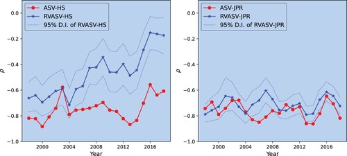
Table 8. The estimated return-volatility correlations for different periods of SPY.

Year	ASV-HS	RVASV-HS	ASV-JPR	RVASV-JPR
1998–2000	−0.819	−0.662	−0.743	−0.788
	[0.054]	[0.058]	[0.080]	[0.035]
	(−0.904, −0.694)	(−0.766, −0.536)	(−0.866, −0.555)	(−0.848, −0.712)
2001–2003	−0.809	−0.651	−0.742	−0.646
	[0.060]	[0.071]	[0.088]	[0.067]
	(−0.903, −0.667)	(−0.777, −0.502)	(−0.875, −0.538)	(−0.766, −0.504)
2004–2007	−0.7887	−0.7162	−0.7703	−0.7834
	[0.072]	[0.060]	[0.083]	[0.044]
	(−0.895, −0.618)	(−0.822, −0.586)	(−0.889, −0.570)	(−0.860, −0.688)
2007–2009	−0.7402	−0.4271	−0.8090	−0.6044
	[0.085]	[0.063]	[0.054]	[0.050]
	(−0.873, −0.544)	(−0.551, −0.303)	(−0.893, −0.685)	(−0.698, −0.504)
2010–2012	−0.7555	−0.4595	−0.7138	−0.7596
	[0.067]	[0.081]	[0.078]	[0.037]
	(−0.864, −0.605)	(−0.612, −0.295)	(−0.841, −0.538)	(−0.825, −0.681)
2013–2015	−0.8673	−0.4859	−0.8602	−0.7909
	[0.039]	[0.076]	[0.042]	[0.031]
	(−0.929, −0.776)	(−0.633, −0.337)	(−0.922, −0.761)	(−0.848, −0.725)
2016–2018	−0.5580	−0.1521	−0.6469	−0.6142
	[0.088]	[0.066]	[0.092]	[0.038]
	(−0.711, −0.370)	(−0.285, −0.025)	(−0.799, −0.445)	(−0.686, −0.536)
2018–2020	−0.6077	−0.1734	−0.8181	−0.7235
	[0.080]	[0.072]	[0.050]	[0.033]
	(−0.750, −0.434)	(−0.320, −0.036)	(−0.895, −0.701)	(−0.785, −0.655)

Note: The table reports the posterior mean, the standard deviation in [] and 0.95 density interval in ().

This table compares the estimated return-volatility correlation coefficients of the ASV-HS, RVASV-HS, ASV-JPR, and RVASV-JPR models for different periods. The estimated ${\rho }_{HS}$ from the RVASV-HS model could change significantly over time. For recent years (from 2016 to 2020), ${\rho }_{HS}$ could be as high as $-0.1521$ while it could be as low as $-0.7162$ for the time range 2004 to 2007. For the ASV-HS, ASV-JPR, and RVASV-JPR models, the estimated ${\rho }_{JPR}$ ranges from $-0.8$ to $-0.6$.

The results show that the lead-lag return-volatility correlation, as specified by the ASV-HS or RVASV-HS model, significantly varies over time when jointly models return an RV as the RVASV-HS model. The estimated ${\rho }_{HS}$ could be as high as $-0.1521$ for the years 2016 to 2018, which suggests a weak or even insignificant.¹⁵ However, from 2004 to 2006, ${\rho }_{HS}$ could be as low as $-0.7162$, which suggests a strong lead-lag return-volatility correlation. On the other hand, the ASV-HS model reports a relatively stable correlation as ${\rho }_{HS}$ ranges between $-0.8$ to $-0.6$. In addition, the contemporaneous return-volatility correlations are consistently around $-0.7$ over the past 20 years for both the ASV-JPR and RVASV-JPR models.

Left graph of figure 1 shows that ASV-HS supports the conclusion that the current return innovation is negatively correlated with future volatility innovations. This correlation has been significant and consistent for the U.S. equity indexes for the past 20 years. By estimating the ASV-HS model with subsamples of different periods, the empirical evidence does not support the time-varying property of the lead-lag return-volatility correlation. However, by jointly modeling the return and ex-post volatility, we find that the return volatility correlation varies from a strong correlation to a weak or insignificant one.

Our simulation studies can explain the mixed evidence provided by ASV-HS and RVASV-HS models. Modeling return series with the ASV-HS model could lead to misidentification of the return-volatility parameter. As figure 1 has shown, the contemporaneous return-volatility correlation is strong and consistent over time. Estimating the ASV-HS model with return alone could lead to a significant lead-lag return-volatility correlation, which may not represent the true relation. As a result, empirical results of the ASV-HS model fail to reveal that the lead-lag return-volatility correlation could depend on the market condition and change significantly over time.

Given both the simulation study and forecasting comparison¹⁶ To support the superiority of jointly estimating return and corresponding volatility measure, the RVASV-HS model (or BVASV-HS model) produces a more accurate estimation of the lead-lag return-volatility correlation and reveals the time-varying property of the ‘leverage effect’. Our result provides direct evidence that the asymmetry is not constant over time and sheds light on further modeling or explaining this time-varying asymmetry.

7. Conclusion

Similar to any empirical study on the correlation of two variables, one needs to observe both the return and volatility process to estimate the correlation accurately in the stochastic volatility models. The ASV model improves the SV model by modeling the asymmetric return-volatility correlation. The ASV model infers the volatility process from the return series according to the model's specification without observing the volatility process. As a result, the ASV model estimates the correlation coefficient between the return and the inferred volatility process, which is endogenous to the return process.

The realized volatility measures allow us to model the return-volatility correlation conditionally by observing both the return and volatility process. Using more than 20 years' daily returns and corresponding RV/BV of three major U.S. equity indexes, we show that incorporating the RV/BV produces a significantly different estimation of the return-volatility correlation, as expected by the simulation study. We conduct out-of-sample comparisons from both return density forecasting and mean-variance portfolio management perspective. The results strongly support the improvement from RVASV-HS and BVASV-HS models, which confirms the accuracy of the return-volatility correlation estimated by jointly modeling return and ex-post volatility. The significant improvement brought by incorporating an accurate volatility measure calls for further development of accurate realized volatility estimations (Fan and Wang 2007, Barndorff-Nielsen et al. 2008, Griffin et al. 2021).

We provide consistent evidence of the time-varying leverage effect for the U.S. equity indexes by jointly modeling return and RV (BV) over sub-samples. Moreover, the misidentification of the ASV-HS model conceals the time-varying properties. Our work provides important evidence for ASV modeling and sheds light on further research.

Disclosure statement

No potential conflict of interest was reported by the author(s).

Supplemental data

Supplemental data for this article can be accessed online at http://dx.doi.org/10.1080/14697688.2022.2140700.

Notes

1 High-frequency-based realized volatility measures (like the realized volatility $R{V}_t$), which will be formally defined in Section 4, suffer from microstructure noise and non-trading hour bias. Takahashi et al. (2009) jointly model daily return and $\log R{V}_t$ and show that the non-trading hour bias is more significant. Shifting $\log R{V}_t$ with constant term ξ assumes that the bias could be adjusted by scaling $R{V}_t$. However, this may not be a valid assumption since the microstructure noise and non-trading hour bias could be autocorrelated, especially when the market is highly volatile or crashes. Equations (9(9) $\begin{array}{rl}{y}_t& =\mu +\exp \left(h_t/2\right)u_t,\\ h_{t+1}& =\delta h_t+v_{t+1},\\ V{M}_t& =\xi +h_t+e_t,e_t\sim N(0,{\sigma }_{VM}^2),\\ \left[\begin{array}{c}{u}_t\\ v_{t+1}\end{array}\right]& \sim \mathit{N}(\left[\begin{array}{c}0\\ 0\end{array}\right],\left[\begin{array}{cc}{\sigma }_y^2& {\rho }_{HS}{\sigma }_y{\sigma }_h\\ {\rho }_{HS}{\sigma }_y{\sigma }_h& {\sigma }_h^2\end{array}\right]).\end{array}$(9) ) and (10(10) $\begin{array}{rl}{y}_t& =\mu +\exp \left(h_t/2\right)u_t,\\ h_t& =\delta h_{t-1}+v_t,\\ V{M}_t& =\xi +h_t+e_t,e_t\sim N(0,{\sigma }_{VM}^2),\\ \left[\begin{array}{c}{u}_t\\ v_t\end{array}\right]& \sim \mathit{N}(\left[\begin{array}{c}0\\ 0\end{array}\right],\left[\begin{array}{cc}{\sigma }_y^2& {\rho }_{JPR}{\sigma }_y{\sigma }_h\\ {\rho }_{JPR}{\sigma }_y{\sigma }_h& {\sigma }_h^2\end{array}\right]).\end{array}$(10) ) could have a missing serial correlated variable, which captures the dynamics of microstructure noise and non-trading hour bias. In this paper, we follow the specification of existing literature, and the assumption of constant ξ and i.i.d $e_t$ does not affect the validity of our findings. Future research might improve the accuracy of realized volatility measures or model the serial correlation of $e_t$.

2 For robustness, we also simulate the symmetry scenario by letting ${\rho }_{HS}$ and ${\rho }_{JPR}$ equal to 0, indicating that the volatility innovation is not related to contemporaneous and lagged return innovations. The empirical results, as shown in table A1 of the Online Appendix, both ASV-HS and ASV-JPR models would correctly identify the correct parameters, as the symmetric SV model is a special case of the ASV-HS or ASV-JPR model.

3 In this section of simulation studies, ${\rho }_{JPR}=-0.113$ indicates that the mean (across simulated samples) of posterior mean is $-0.113$, so do ${\rho }_{HS}$ and other parameters.

4 To rule out the concern that the misidentification could be a result of a divergent MCMC algorithm, in Section A5 of the Online Appendix, we report the trace plots of fitting the ASV-HS (ASV-JPR) model with a random sample of simulated returns where contemporaneous (lead-lag) return-volatility correlation exist. We confirm the convergence of the Bayesian algorithm for both ASV-HS and ASV-JPR models.

5 Greater misspecification means fitting the return with ASV-HS (ASV-JPR) model but there is stronger contemporaneous (lead-lag) return-volatility correlation.

6 Given $y_t$ and $h_t$, both ASV-HS and ASV-JPR model could be estimated as multivariate linear regressions.

7 For comparison, we keep the simulated samples of return and true volatility in Section 3.1 and only simulated volatility measures according to equation (14(14) $\begin{array}{rl}{y}_t& =\mu +\exp \left(h_t/2\right)u_t,u_t\sim N(0,{\sigma }_y^2),\\ h_t& =\delta h_{t-1}+\frac{{\rho }_{JPR}{\sigma }_h}{{\sigma }_y}{u}_t+\frac{{\rho }_{HS}{\sigma }_h}{{\sigma }_y}{u}_{t-1}\\ & +\sqrt{1-{\rho }_{HS}^2-{\rho }_{JPR}^2}{w}_t,w_t\sim N(0,{\sigma }_h^2),\\ V{M}_t& =\xi +h_t+e_t,e_t\sim N(0,{\sigma }_{VM}^2),\end{array}$(14) ).

8 In table A8 of the Online Appendix, we report the estimation results of VMASV-HS and VMASV-JPR models when the return-volatility correlations are consistent with the true model, respectively. Both VMASV-HS and VMASV-JPR models correctly identify all parameters, supporting the validity of our estimation of the VMASV models. Moreover, fitting VMASV models with simulated return and volatility measures leads to a sharpener identification of the common parameters (smaller posterior standard deviations and narrower density intervals).

9 In the Online Appendix, tables A9 and A10 further show the improvements of incorporating the volatility measure in the VMASV-JPR model, which is consistent with the results of the VMASV-HS model in tables 3 and 4. An accurate volatility measure helps the VMASV-JPR model correctly identify the contemporaneous return-volatility correlation, and the noisier volatility measures also significantly mitigate misidentification.

10 Using index returns and the corresponding RV (BV) leads to similar results. However, as Zhang and Zhao (2020) has shown, the open prices of major U.S. equity indexes are misleading due to the casualness of index providers in setting the open prices. The estimated RV and BV, involving open prices of the index, could be too noisy by including false turbulence at the market open.

11 We jointly model the daily close-to-close returns and daily open-to-close RV (BV) to avoid noises from measuring overnight volatilities with squared overnight returns. Our model specification allows overnight bias and noise of the RV or BV.

12 Notice that we do not include the ASV-JPR or VMASV-JPR for forecasting comparison, as the ASV-JPR specification is not a semi-martingale sequence. The conditional return mean is not zero or a constant μ (see Yu 2005 for details).

13 There are about 750 daily observations within each subsample, which is large enough for fitting ASV models. We also test 4-year or 5-year subsamples and the findings are consistent.

14 Using BV as a volatility measure lead to a similar result as that of RV, we only report the estimation results of RVASV-HS and RVASV-JPR here for conciseness.

15 For years 2016 to 2018 (or 2018 to 2020), the 99% density interval of ${\rho }_{HS}$ of RVASV-HS model contains zero.

16 One may concern that our forecasting comparison uses all past observations, i.e., to predict the distribution of one-day-ahead return $y_{i+1}$, we use observations $t=1,2,\dots i$ to fit the models, while the subsample analysis uses 3-year daily observations. We also compare the distributional forecasting of ASV-HS and RVASV-HS models by fitting the model with past 3-year daily observations ($t=i-750,\dots i$). The RVASV-HS model consistently dominates the ASV-HS model.

References

- Ait-Sahalia, Y., Mykland, P.A. and Zhang, L., Ultra high frequency volatility estimation with dependent microstructure noise. J. Econom., 2011, 160(1), 160–175.
- Andersen, T.G. and Bollerslev, T., Answering the skeptics: Yes, standard volatility models do provide accurate forecasts. Int. Econ. Rev., 1998, 39, 885–905.
- Andersen, T.G., Bollerslev, T., Diebold, F.X. and Ebens, H., The distribution of realized stock return volatility. J. Financ. Econ., 2001, 61(1), 43–76.
- Asai, M., Chang, C.-L. and McAleer, M., Realized stochastic volatility with general asymmetry and long memory. J. Econom., 2017, 199(2), 202–212.
- Bandi, F.M. and Russell, J.R., Microstructure noise, realized variance, and optimal sampling. Rev. Econ. Stud., 2008, 75(2), 339–369.
- Barndorff-Nielsen, O.E. and Shephard, N., Non-Gaussian Ornstein-Uhlenbeck-based models and some of their uses in financial economics. J. R. Stat. Soc. Ser. B (Stat. Methodol.), 2001, 63(2), 167–241.
- Barndorff-Nielsen, O.E. and Shephard, N., Econometric analysis of realized volatility and its use in estimating stochastic volatility models. J. R. Stat. Soc. Ser. B (Stat. Methodol.), 2002, 64(2), 253–280.
- Barndorff-Nielsen, O.E. and Shephard, N., Power and bipower variation with stochastic volatility and jumps. J. Financ. Econom., 2004, 2(1), 1–37.
- Barndorff-Nielsen, O.E., Hansen, P.R., Lunde, A. and Shephard, N., Designing realized kernels to measure the ex post variation of equity prices in the presence of noise. Econometrica, 2008, 76(6), 1481–1536.
- Bollerslev, T., Generalized autoregressive conditional heteroskedasticity. J. Econom., 1986, 31(3), 307–327.
- Bollerslev, T., Kretschmer, U., Pigorsch, C. and Tauchen, G., A discrete-time model for daily S&P500 returns and realized variations: Jumps and leverage effects. J. Econom., 2009, 150(2), 151–166.
- Corsi, F., A simple approximate long-memory model of realized volatility. J. Financ. Econom., 2009, 7(2), 174–196.
- Engle, R.F., Autoregressive conditional heteroscedasticity with estimates of the variance of united kingdom inflation. Econometrica, 1982, 50(4), 987–1007.
- Fan, J. and Wang, Y., Multi-scale jump and volatility analysis for high-frequency financial data. J. Am. Stat. Assoc., 2007, 102(480), 1349–1362.
- Gelman, A., Hwang, J. and Vehtari, A., Understanding predictive information criteria for Bayesian models. Stat. Comput., 2014, 24(6), 997–1016.
- Geweke, J. and Amisano, G., Comparing and evaluating Bayesian predictive distributions of asset returns. Int. J. Forecast., 2010, 26(2), 216–230.
- Griffin, J., Liu, J. and Maheu, J.M., Bayesian nonparametric estimation of ex post variance. J. Financ. Econom., 2021, 19(5), 823–859.
- Hansen, P.R. and Lunde, A., A realized variance for the whole day based on intermittent high-frequency data. J. Financ. Econom., 2005, 3(4), 525–554.
- Harvey, A.C. and Shephard, N., Estimation of an asymmetric stochastic volatility model for asset returns. J. Bus. Econ. Statist., 1996, 14(4), 429–434.
- Jacquier, E., Polson, N.G. and Rossi, P.E., Bayesian analysis of stochastic volatility models with fat-tails and correlated errors. J. Econom., 2004, 122(1), 185–212.
- Jensen, M.J. and Maheu, J.M., Estimating a semiparametric asymmetric stochastic volatility model with a dirichlet process mixture. J. Econom., 2014, 178, 523–538.
- Kass, R.E. and Raftery, A.E., Bayes factors. J. Am. Stat. Assoc., 1995, 90(430), 773–795.
- Kim, D. and Kon, S.J., Alternative models for the conditional heteroscedasticity of stock returns. J. Bus., 1994, 67, 563–598.
- Koopman, S.J. and Scharth, M., The analysis of stochastic volatility in the presence of daily realized measures. J. Financ. Econom., 2013, 11(1), 76–115.
- Liu, J. and Maheu, J.M., Improving markov switching models using realized variance. J. Appl. Econom., 2018, 33(3), 297–318.
- Maheu, J.M. and McCurdy, T.H., Do high-frequency measures of volatility improve forecasts of return distributions? J. Econom., 2011, 160(1), 69–76.
- Men, Z., McLeish, D., Kolkiewicz, A.W. and Wirjanto, T.S., Comparison of asymmetric stochastic volatility models under different correlation structures. J. Appl. Stat., 2017, 44(8), 1350–1368.
- Shirota, S., Hizu, T. and Omori, Y., Realized stochastic volatility with leverage and long memory. Comput. Stat. Data. Anal., 2014, 76, 618–641.
- Takahashi, M., Omori, Y. and Watanabe, T., Estimating stochastic volatility models using daily returns and realized volatility simultaneously. Comput. Stat. Data. Anal., 2009, 53(6), 2404–2426.
- Tauchen, G., Zhang, H. and Liu, M., Volume, volatility, and leverage: A dynamic analysis. J. Econom., 1996, 74(1), 177–208.
- Taylor, S.J., Modelling Financial Time Series, 2008 (World Scientific: Singapore).
- Venter, J. and De Jongh, P., Extended stochastic volatility models incorporating realised measures. Comput. Stat. Data. Anal., 2014, 76, 687–707.
- Yu, J., On leverage in a stochastic volatility model. J. Econom., 2005, 127(2), 165–178.
- Zhang, Z. and Zhao, R., Is overnight volatility overlooked? Working Paper, 2020.