Asymmetric short-rate model without lower bound

Abstract

We propose a new short-rate process which appropriately captures the salient features of the negative interest rate environment. The model combines the advantages of the Vasicek and Cox–Ingersoll–Ross (CIR) dynamics: it is flexible, tractable and displays positive skewness without imposing a strict lower bound. In addition, a novel calibration procedure is introduced which focuses on minimizing the Jensen–Shannon (JS) divergence between the model- and market-implied forward rate densities rather than focusing on the minimization of price or volatility discrepancies. A thorough empirical analysis based on cap market quotes shows that our model displays superior performance compared to the Vasicek and CIR models regardless of the calibration method. Our proposed calibration procedure based on the JS divergence better captures the entire forward rate distribution compared to competing approaches while maintaining a good fit in terms of pricing and implied volatility errors.

Keywords:

• Affine short-rate model
• Negative interest rates
• Jensen–Shannon divergence
• Implied density calibration

JEL classifications:

• C52
• C61
• E43
• G12
• G13

1. Introduction

The Global Financial Crisis of 2007–2008 prompted major central banks to cut their policy rates to mitigate the contractionary effects of the crisis on the real economy. Faced with the inability to further decrease their policy rates to support the economic recovery due to the (Zero) Lower Bound constraint, central banks resorted to unconventional monetary policies (UMPs), such as quantitative easing and negative interest rate policies, in an attempt to further stimulate the economic recovery in a low interest rate environment. Research has mainly focused on assessing the effectiveness of UMPs in stimulating the real economy; see e.g. Acharya et al. (2019) for an analysis of the real effects of the ECB's Outright Monetary Transactions (OMT) programme and Heider et al. (2019) for a study of the transmission of negative interest rates to the real economy through the bank lending channel.

Fewer papers focus on the implications of the low interest rate environment, which results partly from UMPs implemented by central banks, for the modelling and pricing of interest rate derivatives. Filipović et al. (2017) introduce the linear-rational term structure framework for the pricing of swaps and European swaptions and Filipović and Kitapbayev (2018) extend it to American swaption pricing. The authors' contributions are, however, limited to an environment with a strict Zero Lower Bound and thus provide limited insights on challenges associated with derivative pricing in a negative interest rate environment. Recchioni et al. (2017) show empirically that allowing for negative interest rates within the multi-factor Heston stochastic volatility model of Recchioni and Sun (2016) leads to more accurate pricing both in-sample and out-of-sample for European call and put equity options.

We make a contribution to this research agenda by developing a short-rate model which appropriately captures the salient features of the negative interest rate environment while delivering tractable semi-analytical expressions for the pricing of caplets. Mean-reverting processes such as the Vasicek model (Vasicek 1977) and the Cox–Ingersoll–Ross model (Cox et al. 1985; CIR hereafter) are considered as standard benchmarks for the modelling of short rate dynamics. The latter was often favoured before the negative interest rate period as it precludes negative values, in contrast to the Vasicek model which postulates a Gaussian distribution. Nevertheless, short-rate modelling frameworks need to be reviewed to better reflect the recent interest rate environment. The most direct solution would be returning to models exhibiting Gaussian dynamics, such as the Vasicek model, which do not preclude negative values. However, this approach might be at odds with empirical evidence as interest rates display conditional asymmetry in their dynamics; see, e.g. Bauer and Chernov (2021) who document pronounced variations in US yield conditional skewness over the business cycle using option-implied skewness for future Treasury yields. Square-root dynamics, as found in the CIR model, can provide the desired positive skewness but at the cost of non-negativity, which is not appropriate in a negative rate environment. A straightforward solution is to introduce a constant negative shift to the CIR process. Nevertheless, the resulting model would exhibit a strict lower bound (the shift itself). In addition, although one could treat the shift as an additional parameter to be estimated from the data, this approach does not prescribe how to reliably estimate this lower bound parameter and guidelines from the empirical or theoretical literature are currently scarce.

In light of these limitations, this paper makes four contributions: first, we propose a two-factor model (VaCIR hereafter) which combines the desirable features of the Vasicek and CIR models. We also consider the deterministic shift extension of these models proposed by Brigo and Mercurio (2001) which guarantees a perfect fit to the term structure of interest rates. The shifted versions of the Vasicek and CIR models are known respectively as the Hull–White model (Hull and White 1990) and the CIR++ model (Brigo and Mercurio 2001). These two models are then combined to obtain the shifted version of our VaCIR model which we denote as VaCIR++. The term structure literature has previously resorted to similar two-factor models to obtain decompositions of risky interest rates into their risk-free components, modelled by a Vasicek process, and compensations for their exposures to credit and/or liquidity risks, modelled by CIR processes; see, for example Longstaff et al. (2005) and Filipović and Trolle (2013). Instead, our purpose is to propose a two-factor approach that would better characterize interest rate dynamics in a negative interest rate environment. The tractability of our framework allows us to obtain semi-analytical expressions for the forward rate density and caplet pricing.

Second, we propose a novel approach to calibrate short-rate models by forward rate density matching. This is achieved by minimizing the distance between the market- and model-implied densities, measured by the Jensen–Shannon (JS) divergence. More precisely, we choose the model parameters such that the associated forward rate distribution, computed under the corresponding forward measure, is the closest to the one implied by derivative market prices. The key advantage over the price or volatility mean squared error (MSE hereafter) minimization is that our approach analyses the fit based on the full distribution rather than focusing on a few data points. An accurate calibration of the density tends to ensure a good fit in terms of prices or volatilities. However, the converse is not necessarily true. Our proposed calibration methodology generalizes moment-based approaches which focus on a few key moments of the distribution—see, for example Guillaume and Schoutens (2013). By focusing on the whole density, our approach accounts for all the moments and circumvents the challenges associated with selecting which moments to match and how to aggregate the matching errors of the various moments into a single one. Furthermore, by switching the focus of the calibration approach to the minimization of the relative entropy (here, the JS divergence) between the market- and model-implied densities, our contribution also builds directly on the literature applying information theory to quantitative finance. Brody and Hughston (2002) propose a calibration methodology based on Shannon entropy maximization which they apply to interest rate term structure models. Cont and Tankov (2004) suggest a regularized calibration approach for exponential Lévy processes to stock option prices based on relative entropy. By contrast, our approach can be applied to any tractable short-rate models, such as the Hull–White and CIR++ models, and extensions such as our proposed VaCIR++ model. Moreover, instead of using the discrepancy between the densities as a penalty to amend the traditional pricing error minimization approach as in Cont and Tankov (2004), it serves as the main objective function in our calibration method. Finally, Tavin (2012) introduces a calibration approach for Normal Inverse Gaussian models to asset log-returns based on relative entropy matching of the risk-neutral density implied by the volatility smile. However, our contribution departs from this one by adopting a model-free approach to infer the implied forward rate density from market data; using the arbitrage-free smoothing technique of the implied-volatility surface of Fengler (2009) to ensure that the forward rate density obtained is well specified; and opting for the Jensen–Shannon divergence which is better suited to compare densities with potentially different supports.

Third, we study the evolution of the market-implied EURIBOR forward rate densities during the recent period of negative interest rates. To this end, we collect a time series of normal volatility curves of caps and apply a stripping procedure to obtain caplet prices. The model-free approach of Breeden and Litzenberger (1978) is then used in combination with the arbitrage-free smoothing technique introduced in Fengler (2009) to get smooth non-negative market implied forward rate densities. These densities are the key input to derivative pricing and will serve as the calibration target in the density matching approach we developed. Two papers propose an analysis related to our empirical study of market-implied forward rate densities: Li and Zhao (2009) study the probability density functions of future US LIBOR rates implied from caps data. Similarly, Trolle and Schwartz (2014) provide stylized facts about higher-order swap rate moments based on the implied density obtained from the swaption cube data for Europe and the USA. However, both papers focus on the period preceding the low interest rate regime and their analysis does not provide relevant insights about the negative interest rate environment.

Fourth, we provide a thorough empirical study investigating the performance of our bivariate VaCIR++ model during the recent period of negative interest rates in the euro area. This is achieved by comparing our model to its single-factor components, the Hull-White and CIR++ models, as well as their two-factor extensions, the G2++ and the CIR2++, respectively. We evaluate the performance of these models when calibrated using both the volatility MSE and density matching criteria. We find that the VaCIR++ model, which combines the features of the Hull–White and CIR++ models, consistently exhibits the best performance regardless of the target criterion. Our results further demonstrate that the JS divergence calibration approach provides a more robust way of calibrating interest rate models to fixed-income derivative data since it has superior performance in capturing the entire forward distribution, high pricing accuracy and comparable fitting quality in terms of matching implied-volatility curves. Therefore, this approach can then be used to price new, complex and illiquid derivatives with the same underlying forward rate.

The remainder of this paper is organized as follows: Section 2 introduces the modelling framework which combines the Hull–White and CIR++ models into our proposed two-factor VaCIR++ model. Section 3 details the different steps of our calibration algorithm. Section 4 presents the data for our empirical application and the results. Section 5 concludes.

2. Model description

In this section, we focus on analytically tractable homogeneous short-rate models existing in the literature and explain how to extend them to obtain a more flexible and general framework that will better account for the negative interest rate environment. For all three considered cases, we use the deterministic shift extension illustrated by Brigo and Mercurio (2001). The idea is that by shifting a latent model with time-homogeneous dynamics with a deterministic function $\varphi :{\mathbb{R}}^{+}\to \mathbb{R}$, one obtains a short-rate model that is analytically tractable and able to perfectly fit the term structure of interest rates. Moreover, the shift function ϕ is directly given by the difference between the instantaneous forward rate curve implied from the market and that generated by the latent process, possibly available in closed form.

We start with two classic short-rate models which will serve as benchmarks. The obvious choice is the Hull–White model. We consider an Ornstein–Uhlenbeck (Gaussian) latent process and shift it with the function ϕ. The other natural candidate is the CIR model. Applying a deterministic shift function to the latter yields the CIR++ model. This model features skewness and is compatible with the negative rates environment thanks to the shift. Note that this model exhibits a strict lower bound up to any time horizon T, given by the minimum of the function ϕ on the interval $[0,T]$. The alternative we propose is a combination of the aforementioned models, in an attempt to address their documented shortcomings while preserving the desired features.

2.1. Baseline framework

We postulate a filtered probability space $(\mathrm{\Omega },\mathcal{F},\mathbb{F},\mathbb{Q})$ where $\mathbb{Q}$ is a probability measure and $\mathbb{F}:=({\mathcal{F}}_t{)}_{t\ge 0}$ the filtration, satisfying the usual conditions. All processes considered in this paper are assumed to be $\mathbb{F}$-adapted.

We consider two standard interest-rate models that we take as benchmarks, namely the Vasicek model (noted x hereafter) and the CIR model (noted y hereafter). The short-rate dynamics are respectively given by (1) $\begin{array}{rl}\mathrm{d}{x}_t& ={\kappa }_1({\theta }_1-x_t)\mathrm{d}t+{\sigma }_1\mathrm{d}{W}_t^x,x_0\in \mathbb{R},\end{array}$(1) (2) $\begin{array}{rl}\mathrm{d}{y}_t& ={\kappa }_2({\theta }_2-y_t)\mathrm{d}t+{\sigma }_2\sqrt{y_t}\mathrm{d}{W}_t^y,y_0\in {\mathbb{R}}_0^{+}.\end{array}$(2) where $W^x$ and $W^y$ are two independent Brownian motions under $\mathbb{Q}$.

These models belong to the class of homogeneous one-factor affine diffusions, with dynamics¹ (3) $\begin{array}{r}\mathrm{d}{z}_t=(a+b{z}_t)\mathrm{d}t+\sqrt{c+d{z}_t}\mathrm{d}{W}_t,z_0>-c/d,\mathrm{\forall }d>0,\end{array}$(3) where W is a Brownian motion. We denote the parameters as $\mathrm{\Psi }=(a,b,c,d,z_0)$. Duffie and Kan (1996) provide conditions to ensure strictly positive volatility of multivariate affine diffusions. In the univariate case, these conditions reduce to $\mathrm{\forall }{z}_t\mathrm{s}.\mathrm{t}.c+d{z}_t=0,d(b{z}_t+a)>\frac{d^2}{2}\iff ad-bc>\frac{d^2}{2}.$ Intuitively, this condition ensures that the boundary (i.e. the value of the process associated with the vanishing square-root condition, $z_t=-c/d$) will never be hit if the drift of the process, i.e. $a+b{z}_t$, is sufficiently positive in the neighbourhood of the boundary. The stochastic differential equations (SDEs) associated with the Vasicek and CIR models are recovered from equation (3(3) $\begin{array}{r}\mathrm{d}{z}_t=(a+b{z}_t)\mathrm{d}t+\sqrt{c+d{z}_t}\mathrm{d}{W}_t,z_0>-c/d,\mathrm{\forall }d>0,\end{array}$(3) ) using respectively ${\mathrm{\Psi }}^x:=({\kappa }_1{\theta }_1,-{\kappa }_1,{\sigma }_1^2,0,x_0)$ and ${\mathrm{\Psi }}^y:=({\kappa }_2{\theta }_2,-{\kappa }_2,0,{\sigma }_2^2,y_0)$.² For the Vasicek model, the condition above is satisfied as $ad-bc={\kappa }_1{\sigma }_1^2>0=\frac{d^2}{2}$. For the CIR model, we have $ad-bc={\kappa }_2{\theta }_2{\sigma }_2^2>\frac{{\sigma }_2^4}{2}=\frac{d^2}{2}$. This is equivalent to the Feller condition ${\kappa }_2{\theta }_2>\frac{{\sigma }_2^2}{2}$, of which the condition in Duffie and Kan (1996) is a multidimensional extension.

Homogeneous affine diffusions, as in equation (3(3) $\begin{array}{r}\mathrm{d}{z}_t=(a+b{z}_t)\mathrm{d}t+\sqrt{c+d{z}_t}\mathrm{d}{W}_t,z_0>-c/d,\mathrm{\forall }d>0,\end{array}$(3) ), are popular due to their analytical tractability which simplifies model calibration. For instance, denoting by $\mathbb{E}$ the expectation under $\mathbb{Q}$, it is well known that for such processes, (4) $\begin{array}{r}{P}_t^z\left(T\right):=\mathbb{E}\left[{\mathrm{e}}^{-{\int }_t^T{z}_s\mathrm{d}s}|{\mathcal{F}}_t\right]=A^z(T-t){\mathrm{e}}^{-B^z(T-t)z_t},\end{array}$(4) where $A^z,B^z$ are deterministic functions satisfying Riccati equations, for which analytical solutions can be found.³

When $\mathbb{Q}$ stands for the risk-neutral measure, $\mathbb{F}$ is the information flow available to investors and z depicts the short-rate process, $P_t^z\left(T\right)$ agrees with $P_t\left(T\right)$, the no-arbitrage price at time t of a risk-free zero-coupon bond with maturity $T\ge t$: (5) $\begin{array}{r}{P}_t\left(T\right):=\mathbb{E}\left[\frac{M_t^z}{M_T^z}|{\mathcal{F}}_t\right]=\mathbb{E}\left[{\mathrm{e}}^{-{\int }_t^T{z}_s\mathrm{d}s}|{\mathcal{F}}_t\right]=P_t^z\left(T\right),\end{array}$(5) where $M^z:=(M_t^z{)}_{t\ge 0}$ and $M_t^z:={\mathrm{e}}^{{\int }_0^t{z}_s\mathrm{d}s}$ is the money market account numéraire.

The existence of analytical expressions for zero-coupon bond prices explains why the Vasicek and CIR models are so popular for interest rate modelling. Furthermore, their deterministic shift extensions make it possible to replicate the observed term structure of discount factors at time t. More specifically, the short rate is expressed as $z_t^{\varphi }=z_t+{\varphi }^z\left(t\right)$, $z\in \{x,y\}$. The corresponding zero-coupon bond price takes the form (6) $\begin{array}{r}{P}_t^{z^{\varphi }}\left(T\right)=\exp \{-{\int }_t^T{\varphi }^z(s\left)\mathrm{d}s\right\}{P}_t^z\left(T\right).\end{array}$(6) One can then choose the function ${\varphi }^z$ such that the discount curve implied by the $z^{\varphi }$ model perfectly agrees with the market discount curve, i.e. $P_t^{z^{\varphi }}\left(T\right)=P_t^M\left(T\right)$. It can be shown that this choice corresponds to (7) $\begin{array}{rl}{\varphi }^z\left(t\right)& =f_0^M\left(t\right)-f_0^z\left(t\right),\end{array}$(7) (8) $\begin{array}{rl}{f}_0^x\left(t\right)& =(\frac{{\sigma }_1^2}{2{\kappa }_1^2}{\mathrm{e}}^{-{\kappa }_{1}t}+\frac{{\kappa }_1^2{\theta }_1-{\sigma }_1^2/2}{{\kappa }_1^2})(1-{\mathrm{e}}^{-{\kappa }_{1}t})+x_0{\mathrm{e}}^{-{\kappa }_{1}t},\end{array}$(8) (9) $\begin{array}{rl}{f}_0^y\left(t\right)& =\frac{2{\kappa }_2{\theta }_2({\mathrm{e}}^{th}-1)}{2h+({\kappa }_2+h)({\mathrm{e}}^{th}-1)}+y_0\frac{4h^2{\mathrm{e}}^{th}}{[2h+({\kappa }_2+h\left)\right({\mathrm{e}}^{th}-1){]}^2},\end{array}$(9) where $f_t^M(\cdot )$ is the time-t instantaneous forward curve associated with the current market term structure, $f_t^z(\cdot )$ is the corresponding curve implied by the model $z\in \{x,y$} and $h:=\sqrt{{\kappa }_2^2+2{\sigma }_2^2}$.

2.2. Proposed extension

Recall that our goal is to design a model that would comply with negative interest rates. As discussed in the introduction, the Vasicek model (x) has the ability to deal with negative values, but at the expense of assuming a Normal distribution for the short rate. The shifted CIR model may comply with the negative interest rate environment whenever the shift is negative. However, as explained above, such a process would exhibit a time-dependent lower bound (the shift function itself) which would be associated with additional challenges on how to reliably estimate a meaningful lower bound on interest rates from available data.

The model we propose aims at capturing skewness without imposing a strict lower bound by combining two latent processes: a Vasicek process and a CIR process. We denote the resulting model VaCIR hereafter. Mathematically, we consider the following dynamics for the short rate in this model: (10) $\begin{array}{r}{r}_t:=x_t+y_t,\end{array}$(10) where the Brownian motions $W^x,W^y$ in equations (1(1) $\begin{array}{rl}\mathrm{d}{x}_t& ={\kappa }_1({\theta }_1-x_t)\mathrm{d}t+{\sigma }_1\mathrm{d}{W}_t^x,x_0\in \mathbb{R},\end{array}$(1) ) and (2(2) $\begin{array}{rl}\mathrm{d}{y}_t& ={\kappa }_2({\theta }_2-y_t)\mathrm{d}t+{\sigma }_2\sqrt{y_t}\mathrm{d}{W}_t^y,y_0\in {\mathbb{R}}_0^{+}.\end{array}$(2) ) are assumed to be independent. This assumption preserves the analytical tractability of zero-coupon bond prices (11) $\begin{array}{rl}{P}_t^r\left(T\right)& =P_t^x\left(T\right)P_t^y\left(T\right)\\ & =A^x(T-t)A^y(T-t){\mathrm{e}}^{-\left[B^x\right(T-t)x_t+B^y(T-t\left)y_t\right]}.\end{array}$(11) Similarly, we extend the combined VaCIR model to perfectly replicate the current observed discount curve (denoted VaCIR++ hereafter), i.e.$r_t^{\varphi }=r_t+{\varphi }^r\left(t\right)$, where ${\varphi }^r\left(t\right)={\varphi }^x\left(t\right)+{\varphi }^y\left(t\right)-f_0^M\left(t\right)$. Additionally, the zero-coupon bond is defined in the same way as in equation (6(6) $\begin{array}{r}{P}_t^{z^{\varphi }}\left(T\right)=\exp \{-{\int }_t^T{\varphi }^z(s\left)\mathrm{d}s\right\}{P}_t^z\left(T\right).\end{array}$(6) ). Introducing correlation between the two latent processes would come at the cost of analytical tractability of A, B since the resulting model would not be part of the affine model class, see appendix 3 for details. One consequence of assuming independence between x and y is that our proposed model might yield unsatisfactory calibration results for the term structure of caplet volatilities exhibiting a large hump shape. As the main focus of our analysis is not the calibration of the market-implied volatility surface, we leave these considerations for future research and refer the interested reader to chapter 4 of Brigo and Mercurio (2007) for more details.

2.3. Forward rate dynamics and densities under the forward measure

Due to the central role played by the forward rate in the price of derivative products (e.g. caps and floors), we derive the dynamics and densities related to the forward rate in the various models⁴ (12) $\begin{array}{r}{F}_t^z(T,S)=\frac{1}{\mathrm{\Delta }}(\frac{P_t^z\left(T\right)}{P_t^z\left(S\right)}-1),z\in \{x,y,r\}.\end{array}$(12) For convenience, we formulate the dynamics of $F(T,S)=\left(F_t\right(T,S){)}_{0\le t\le T<S}$ under the S-forward measure, ${\mathbb{Q}}^S$.

Proposition 1

Let $t\le T<S$ and $\mathrm{\Delta }:=S-T$. Then,

1. The forward rate $F^r(T,S)$ associated with the model specified in equation (10(10) $\begin{array}{r}{r}_t:=x_t+y_t,\end{array}$(10) ) reads as (13) $\begin{array}{r}{F}_t^r(T,S)=\frac{1}{\mathrm{\Delta }}\left(\right(1+\mathrm{\Delta }{F}_t^x(T,S)\left)\right(1+\mathrm{\Delta }{F}_t^y(T,S))-1).\end{array}$(13) Moreover, let ${\sigma }_t^x:={\sigma }_1$, ${\sigma }_t^y:={\sigma }_2\sqrt{y_t}$ be the diffusion coefficients associated with models x and y, respectively. For $z\in \{x,y\}$, define $W_t^{z,S}:=W_t^z+{\int }_0^t{\zeta }_s^{z,S}\mathrm{d}s$ with ${\zeta }_t^{z,S}:={\sigma }_t^z{B}^z(S-t)$. Define ${\mathbb{Q}}^S$ using the random variable ${\frac{\mathrm{d}{\mathbb{Q}}^S}{\mathrm{d}\mathbb{Q}}|}_{{\mathcal{F}}_S}=\frac{P_S^r\left(S\right)}{P_0^r\left(S\right)}\frac{M_0^r}{M_S^r}=\frac{P_S^r\left(S\right)}{P_0^r\left(S\right)M_S^r}.$ Then,

2. $F^x(T,S),F^y(T,S)$ and $F^r(T,S)$ are ${\mathbb{Q}}^S$-martingales;

3. The dynamics of the forward rates associated with x and y are given by (14) $\begin{array}{rl}\mathrm{d}{F}_t^x(T,S)& ={\sigma }^x(t,F_t^x(T,S\left)\right)\mathrm{d}{W}_t^{x,S},\mathrm{d}{F}_t^y(T,S)\\ & ={\sigma }^y(t,F_t^y(T,S\left)\right)\mathrm{d}{W}_t^{y,S},\end{array}$(14) where $W^{x,S},W^{y,S}$ are independent ${\mathbb{Q}}^S$-Brownian motions and $\begin{array}{rl}{\sigma }^x(t,u)& :={\sigma }_1[u+\frac{1}{\mathrm{\Delta }}]\left(B^x\right(S-t)-B^x(T-t\left)\right),\\ {\sigma }^y(t,u)& :={\sigma }_2[u+\frac{1}{\mathrm{\Delta }}]\\ & \times \sqrt{\left(B^y\right(S-t)-B^y(T-t\left)\right)\left(G_t\right(T,S,u\left)\right)},\\ G_t(T,S,u)& :=\ln \left([1+\mathrm{\Delta }u]\frac{A^y(S-t)}{A^y(T-t)}\right).\end{array}$

Proof.

See appendix 4.

Because these processes are independent, the conditional density of $r_t$ given $(x_s,y_s)$ is obtained by the convolution of the corresponding conditional densities for the Vasicek and CIR processes sampled at t. The ${\mathbb{Q}}^S$-conditional densities of x and y can be found in Brigo and Mercurio (2007).

Proposition 2

Let $t\le T\le S$. Under ${\mathbb{Q}}^S$, the density of the spot rate $z_T^{\varphi }$ conditional on $z_t^{\varphi }$, for $z\in \{x,y,r\}$, is given by, (15) $\begin{array}{r}{f}_{z_T^{\varphi }|z_t^{\varphi }}^S\left(u\right)=f_{z_T|z_t}^S(u-{\varphi }^z(t\left)\right).\end{array}$(15) Note that when z = r, the condition $z_T|z_t$ becomes $r_T|(x_t,y_t)$.

1. The density of $x_T$ conditional on $x_t$ is given by (16) $\begin{array}{rl}{f}_{x_T|x_t}^S\left(u\right)& =\frac{1}{{\sigma }^x(T-t)}\phi \left(\frac{u-{\mu }^x(t,T)}{{\sigma }^x(T-t)}\right),\\ {\mu }^x(t,T)& =x_t{\mathrm{e}}^{-{\kappa }_1(T-t)}+M^S(t,T),\\ {\sigma }^x\left(\tau \right)& =\sqrt{\frac{{\sigma }_1^2}{2{\kappa }_1}[1-{\mathrm{e}}^{-2{\kappa }_1\tau }]},\\ M^S(t,T)& =({\theta }_1-\frac{{\sigma }_1^2}{{\kappa }_1^2})(1-{\mathrm{e}}^{-{\kappa }_1(T-t)})\\ & +\frac{{\mathrm{e}}^{-{\kappa }_1(S-T)}}{{\kappa }_1}\left({\sigma }^x\right(T-t){)}^2,\end{array}$(16) where φ is the standard Normal density.

2. The density of $y_T$ conditional on $y_t$ is given by (17) $\begin{array}{rl}{f}_{y_T|y_t}^S\left(u\right)& =f_{{\chi }^2(\nu ,\delta (t,T,S\left)\right)/q(t,T,S)}\left(u\right)\\ & =q(t,T,S)f_{{\chi }^2(\nu ,\delta (t,T,S\left)\right)}\left(q\right(t,T,S\left)u\right),u\ge 0,\end{array}$(17) where $f_{{\chi }^2(\nu ,\delta )}$ is the density of a non-central chi-squared random variable with ν degrees of freedom and non-centrality parameter δ. We introduced the following notation: $\begin{array}{rl}q(t,T,S)& :=2\left(\rho \right(T-t)+\frac{{\kappa }_2+h}{{\sigma }_2^2}+B^y(\mathrm{\Delta }\left)\right),\\ \delta (t,T,S)& :=\frac{4\rho (T-t{)}^2{y}_t{\mathrm{e}}^{h(T-t)}}{q(t,T,S)},\\ \rho \left(\tau \right)& :=\frac{2h}{{\sigma }_2^2(\exp [h\tau ]-1)},\end{array}$ with $\nu :=4{\kappa }_2{\theta }_2/{\sigma }_2^2$ and $h:=\sqrt{{\kappa }_2^2+2{\sigma }_2^2}$.

3. The density of $r_T$ conditional on $(x_t,y_t)$ is given by (18) $\begin{array}{r}{f}_{r_T|(x_t,y_t)}^S\left(u\right)={\int }_0^{\mathrm{\infty }}{f}_{x_T|x_t}^S(u-v)f_{y_T|y_t}^S\left(v\right)\mathrm{d}v.\end{array}$(18)

From the expressions in Proposition 2, we can now provide a characterization of the conditional density of the zero-coupon bond price under the S-forward measure.

Proposition 3

Let $t\le T\le S$. Under ${\mathbb{Q}}^S$, the density of the zero-coupon bond price, $P_T^{z^{\varphi }}\left(S\right)$, conditional upon $z_t^{\varphi }$, for models of $z\in \{x,y,r\}$ with shift extensions, is given by (19) $\begin{array}{r}{f}_{P_T^{z^{\varphi }}\left(S\right)|z_t^{\varphi }}^S\left(u\right)={\mathrm{e}}^{{\int }_t^T{\varphi }^z\left(s\right)\mathrm{d}s}{f}_{P_T^z\left(S\right)|z_t}^S\left(u{\mathrm{e}}^{{\int }_t^T{\varphi }^z\left(s\right)\mathrm{d}s}\right),u\ge 0.\end{array}$(19) Note that when z = r, the condition $P_T^z\left(S\right)|z_t$ becomes $P_T^r\left(S\right)|(x_t,y_t)$.

1. The density of the zero-coupon bond price $P_T^z\left(S\right)$ conditional upon $z_t$, for the Vasicek model (z = x) and the CIR model (z = y) is given by (20) $\begin{array}{r}{f}_{P_T^z\left(S\right)|z_t}^S\left(u\right)=\frac{1}{u{B}^z\left(\mathrm{\Delta }\right)}{f}_{z_T|z_t}^S(\frac{1}{B^z\left(\mathrm{\Delta }\right)}\ln \frac{A^z\left(\mathrm{\Delta }\right)}{u}),\end{array}$(20) where $u\ge 0$ for the Vasicek model and $0\le u\le 1$ for the CIR model. As for the combined model, it reads as (21) $\begin{array}{r}{f}_{P_T^r\left(S\right)|{\mathcal{F}}_t}^S\left(u\right)={\int }_0^1\frac{1}{v}{f}_{P_T^x\left(S\right)|x_t}^S\left(u/v\right)f_{P_T^y\left(S\right)|y_t}^S\left(v\right)\mathrm{d}v,u\ge 0.\end{array}$(21)

2. The density of the spot rate $L^{z^{\varphi }}(T,S):=F_T^{z^{\varphi }}(T,S)$ conditional upon ${\mathcal{F}}_t={\mathcal{F}}_t^x\vee {\mathcal{F}}_t^y$,⁵ $z\in \{x,y,r\}$, is given by (22) $\begin{array}{r}{f}_{L^{z^{\varphi }}(T,S)|{\mathcal{F}}_t}^S\left(u\right)=\frac{\mathrm{\Delta }}{(1+\mathrm{\Delta }u{)}^2}{f}_{P_T^{z^{\varphi }}\left(S\right)|{\mathcal{F}}_t}^S\left(\frac{1}{1+\mathrm{\Delta }u}\right).\end{array}$(22)

3. Model calibration

Calibrating a short-rate model z to the market amounts to (i) selecting a set of n financial products, called calibration instruments hereafter, and (ii) looking for the set of parameters ${\mathrm{\Psi }}^z$ minimizing the discrepancies between the market- and model-implied prices of the calibration instruments. The time-t no-arbitrage price of a caplet on the spot rate $L(T,S)=F_T(T,S)$, with strike K, fixing date T and payment date S>T can be obtained from the ${\mathbb{Q}}^S$ density of $L(T,S)$: (23) $\begin{array}{rl}{\mathrm{C}\mathrm{p}\mathrm{l}}_t(T,S,K)& =M_t\mathbb{E}\left[\frac{\left(L\right(T,S)-K{)}^{+}\mathrm{\Delta }}{M_S}|{\mathcal{F}}_t\right]\\ & =P_t\left(S\right){\mathbb{E}}^S\left[\left(L\right(T,S)-K{)}^{+}\mathrm{\Delta }|{\mathcal{F}}_t\right]\\ & =\mathrm{\Delta }{P}_t\left(S\right){\int }_K^{+\mathrm{\infty }}(v-K)f_{L(T,S)|{\mathcal{F}}_t}^S\left(v\right)\mathrm{d}v,\end{array}$(23) where $P_t\left(S\right)$ is the price of the zero-coupon bond with maturity S at time t and $f_{L(T,S)}^S$ is the density of the spot rate $L(T,S)$ provided in equation (22(22) $\begin{array}{r}{f}_{L^{z^{\varphi }}(T,S)|{\mathcal{F}}_t}^S\left(u\right)=\frac{\mathrm{\Delta }}{(1+\mathrm{\Delta }u{)}^2}{f}_{P_T^{z^{\varphi }}\left(S\right)|{\mathcal{F}}_t}^S\left(\frac{1}{1+\mathrm{\Delta }u}\right).\end{array}$(22) ). The model prices are obtained by evaluating the right-hand side of equation (23(23) $\begin{array}{rl}{\mathrm{C}\mathrm{p}\mathrm{l}}_t(T,S,K)& =M_t\mathbb{E}\left[\frac{\left(L\right(T,S)-K{)}^{+}\mathrm{\Delta }}{M_S}|{\mathcal{F}}_t\right]\\ & =P_t\left(S\right){\mathbb{E}}^S\left[\left(L\right(T,S)-K{)}^{+}\mathrm{\Delta }|{\mathcal{F}}_t\right]\\ & =\mathrm{\Delta }{P}_t\left(S\right){\int }_K^{+\mathrm{\infty }}(v-K)f_{L(T,S)|{\mathcal{F}}_t}^S\left(v\right)\mathrm{d}v,\end{array}$(23) ), replacing $f_{L(T,S)}^S$ by $f_{L^z(T,S)}^S$ in proposition 3 for each of the considered models. Calibration based on the minimization of the mean squared error of implied volatilities is often favoured in practice and we cover this approach in section 3.1. In section 3.2, we introduce a novel calibration technique whose aim is to minimize the distance between the model-implied density, $f_{L^z(T,S)}^S$, and the market-implied one, $f_{L(T,S)}^S$.

3.1. Calibration of the implied-volatility curve

The caplet pricing equation provides us with the formula to compute the caplet prices under the three considered models by plugging in the density function specified in equation (22(22) $\begin{array}{r}{f}_{L^{z^{\varphi }}(T,S)|{\mathcal{F}}_t}^S\left(u\right)=\frac{\mathrm{\Delta }}{(1+\mathrm{\Delta }u{)}^2}{f}_{P_T^{z^{\varphi }}\left(S\right)|{\mathcal{F}}_t}^S\left(\frac{1}{1+\mathrm{\Delta }u}\right).\end{array}$(22) ). Under the assumption of normal volatility and the Bachelier formula, we can obtain the implied volatility associated with caplet products. Based on the implied volatility, the considered models are calibrated to the market caplet volatility surface, and the fitting performance is measured in terms of the mean squared error (MSE) of implied volatilities. We thus calibrate each of the considered models by looking for the parameters ${\mathrm{\Psi }}^z$ which minimize the MSE between the model-implied and market-implied volatilities: (24) $\begin{array}{r}{\mathrm{\Psi }}^{z^{\ast }}:=\arg \underset{{\mathrm{\Psi }}^z}{min}\frac{1}{n}\sum _{i=1}^n{({\sigma }_i^M-{\sigma }_i^z)}^2\end{array}$(24) where ${\sigma }_i^M$ and ${\sigma }_i^z$ are the market- and model-implied volatilities for caplet i, respectively.

3.2. Calibration of the forward rate density

The caplet pricing equation allows us to infer the implied forward rate density from market data in a model-free way.⁶ Indeed, differentiating twice the expression for the caplet price in equation (23(23) $\begin{array}{rl}{\mathrm{C}\mathrm{p}\mathrm{l}}_t(T,S,K)& =M_t\mathbb{E}\left[\frac{\left(L\right(T,S)-K{)}^{+}\mathrm{\Delta }}{M_S}|{\mathcal{F}}_t\right]\\ & =P_t\left(S\right){\mathbb{E}}^S\left[\left(L\right(T,S)-K{)}^{+}\mathrm{\Delta }|{\mathcal{F}}_t\right]\\ & =\mathrm{\Delta }{P}_t\left(S\right){\int }_K^{+\mathrm{\infty }}(v-K)f_{L(T,S)|{\mathcal{F}}_t}^S\left(v\right)\mathrm{d}v,\end{array}$(23) ) with respect to the strike K, we obtain (25) $\begin{array}{r}{f}_{L(T,S)|{\mathcal{F}}_t}^S\left(K\right)=\frac{\frac{{\mathrm{\partial }}^2}{\mathrm{\partial }{K}^2}{\mathrm{C}\mathrm{p}\mathrm{l}}_t(T,S,K)}{\mathrm{\Delta }{P}_t\left(S\right)}.\end{array}$(25) To get an accurate estimation of the density based on equation (25(25) $\begin{array}{r}{f}_{L(T,S)|{\mathcal{F}}_t}^S\left(K\right)=\frac{\frac{{\mathrm{\partial }}^2}{\mathrm{\partial }{K}^2}{\mathrm{C}\mathrm{p}\mathrm{l}}_t(T,S,K)}{\mathrm{\Delta }{P}_t\left(S\right)}.\end{array}$(25) ), we need to obtain the market discount curve and the price quotations for caplets on a fine grid of strikes. Since only a limited number of products are actively traded and quoted on the fixed-income market, we have to resort to interpolation methods. Special care needs to be taken to obtain a valid (i.e. non-negative) and smooth density.

To this end, we use the arbitrage-free smoothing technique of the implied volatility surface developed by Fengler (2009) which we apply to the caplet prices. The procedure takes the quoted caps data and obtains the caplet prices via caplet stripping. Then, a cubic spline smoothing technique is applied to caplet prices, augmented with appropriately chosen linear constraints to enforce no-arbitrage restrictions. By eliminating arbitrage opportunities, this approach precludes the occurrence of negative local volatilities or negative transition probabilities and thus ensures that the forward rate density is well specified.⁷ The method proposed by Fengler (2009) is closely related to the literature on non-parametric estimation of risk-neutral transition densities under shape constraints (Aït-Sahalia and Duarte 2003, Yatchew and Härdle 2006). We decided to adopt it instead of other competing approaches due to its ease of implementation; its good theoretical properties—inherited from the theory on natural smoothing splines under suitable shape constraints; and its applicability in contexts with scarce calibration data. See also Tavin (2012) for alternative approaches to the smoothing of the implied-volatility surface which do not preclude the presence of arbitrage opportunities and impose stronger parametric restrictions on the modelling.

To calibrate the model-implied density to match the market-implied one, we need a criterion assessing how far the model-implied density is from the reference one. A common approach taken in the literature relies on a moment-based approach which focuses on a few key moments of the distribution (Guillaume and Schoutens 2013). This problem has also been tackled by adopting an information-theoretic point of view, in which all moments are taken into account. In particular, Cont and Tankov (2004) introduce a regularization term based on relative entropy in a calibration problem based on MAE minimization to enforce uniqueness and stability of the solution. See also Brody and Hughston (2002) for an application of the Shannon entropy to term structure modelling. We build on this existing literature and select the measure based on Kullback–Leibler (KL) divergence as our calibration criteria.⁸ ${}^{,}$⁹ Specifically, the KL divergence between two densities $(p,q)$ is the relative entropy, and is based on (differential) Shannon's entropy: (26) $\begin{array}{r}〈p|q〉:=\int p\left(x\right)\log \left(\frac{p\left(x\right)}{q\left(x\right)}\right)\mathrm{d}x,\end{array}$(26) where p is assumed to be absolutely continuous with respect to q.

Note that, given the asymmetry of the KL divergence, $〈p|q〉$ will typically be different from $〈q|p〉$. As a consequence, basing the optimization program on only one of them would result in different outcomes. Additionally, optimization based on the KL divergence might face some challenges in practice as the KL divergence is not defined when p is not absolutely continuous with respect to q. In our application, we circumvent these issues by considering the Jensen--Shannon (JS) divergence which is a symmetrized and smoothed version of the KL divergence. Specifically, the JS divergence between two densities $(p,q)$ is defined as (27) $\begin{array}{r}\mathrm{JSD}\left(p|q\right)=\frac{1}{2}〈p|m〉+\frac{1}{2}〈q|m〉,\end{array}$(27) where $m=\frac{1}{2}(p+q)$. By comparing both densities to their average, the JS divergence is always ensured to be bounded as the denominator in the log is always nonzero whenever the numerator is nonzero. Therefore, the JS divergence can be used to compare densities with different supports. Additionally, the measure is bounded at zero and reaches this lower bound only when p = q almost everywhere.

Equipped with a measure accurately quantifying the goodness of fit between densities, we can calibrate each of the considered models by choosing as parameters the set ${\mathrm{\Psi }}^z$ which minimize the JS divergence between the model-implied and the market-implied densities (28) $\begin{array}{r}{\mathrm{\Psi }}^{z^{\ast }}:=\arg \underset{{\mathrm{\Psi }}^z}{min}JSD\left(f_{L(T,S)}^S|f_{L^z(T,S)}^S\right)\end{array}$(28) where $f_{L(T,S)}^S$ and $f_{L^z(T,S)}^S$ are respectively the market- and model-implied forward rate densities.

3.3. Summary of calibration algorithm

As summarized in the diagram 3.3, we use algorithm 1 and algorithm 2 to calibrate the model over a discrete grid of strikes $K\in \{K_0,K_1,K_2\dots K_{N-1},K_N\}$ for certain lower and upper bounds of $K_0$ and $K_N$.¹⁰

3.4. Multi-period extension

The calibration approach outlined in section 3.2 only considers caplet products with a single pair of fixing and payment dates $(T,S)$ for different strikes $K\in \{K_0,K_1,\dots ,K_N\}$ whose underlyings correspond to the same spot rate $L(T,S)$. One might also be interested in pricing multiple caplet products with different fixing and payment dates using a common short-rate model. Although several routes are possible, this can be easily achieved with the following two-step procedure. First, we retrieve caplet prices for products with pairs of fixing and payment dates denoted by $(T^i,S^i),i=1,\dots ,M$, for different strikes $K^i\in \{K_0^i,K_1^i,\dots ,K_{N^i}^i\}$ from market cap data using caplet stripping and we construct the caplet price curve for a finer grid of strikes via the arbitrage-free smoothing technique of the implied-volatility surface (Fengler 2009). Second, we can calibrate each of the considered short-rate models by choosing the set of parameters ${\mathrm{\Psi }}^z$ which minimizes the sum of all JS divergence (29) $\begin{array}{r}{\mathrm{\Psi }}^{z^{\ast }}:=\arg \underset{{\mathrm{\Psi }}^z}{min}\sum _{i=1}^{M}JSD\left(f_{L(T^i,S^i)}^{S^i}|f_{L^z(T^i,S^i)}^{S^i}\right)\end{array}$(29) where $JSD\left(f_{L(T^i,S^i)}^{S^i}|f_{L^z(T^i,S^i)}^{S^i}\right)$ is the JS divergence value between the market- and model-implied densities for the corresponding spot rates $L(T^i,S^i)$. A weighting scheme could further be applied to the elements of the sum in equation (29(29) $\begin{array}{r}{\mathrm{\Psi }}^{z^{\ast }}:=\arg \underset{{\mathrm{\Psi }}^z}{min}\sum _{i=1}^{M}JSD\left(f_{L(T^i,S^i)}^{S^i}|f_{L^z(T^i,S^i)}^{S^i}\right)\end{array}$(29) ) to reflect, e.g. relative differences in liquidity across fixing and payment dates.

4. Empirical application

In this section, we present an empirical application where we conduct a thorough performance comparison of the three competing models (namely, Hull–White, CIR++ and VaCIR++) under the two calibration schemes introduced in section 3. More specifically, we take the 6-month forward rate as an example to evaluate the pricing accuracy and the quality of fitting the market-implied-volatility curve. We further investigate the distribution of the forward rate in 6 months and illustrate the model performance in terms of density matching under the three considered frameworks in the negative interest rate environment. The rest of this section is organized as follows: section 4.1 presents the data description and sample coverage used for our empirical application and illustrates the non-arbitrage smoothing technique implemented to construct the market-implied density curve; Section 4.2 covers the calibration results based on the minimization of implied volatility errors; Section 4.3 covers the calibration results based on the minimization of JS divergence where the modelled forward density is matched to the market-implied one.

4.1. Data description and volatility curve smoothing

We use historical data for the 6-month EURIBOR forward rate $F_0(6M,1Y)$ and the interest rate derivatives whose underlying rate is the 6-month forward rate in 6 months, i.e. $L(6M,1Y)=F_{6M}(6M,1Y)$.¹¹ Observe that the market provides quotations for the implied volatilities of caps whereas, to compute the market-implied density for the forward rate $L(6M,1Y)$, we need caplet prices associated with the latter.

Therefore, we start by collecting monthly normal volatility quotes from Refinitiv (formerly known as Eikon, Thomson Reuters) for the 6-month EURIBOR caps quoted over a grid composed of 13 different strikes. The sample period spans from March 31, 2016, to January 29, 2021, during which the 6-month EURIBOR and 6-month forward rate are in the negative territory. Then we use the Bachelier formula to get the cap prices and apply the stripping approach proposed in Hagan and Konikov (2004) to extract caplet prices.

The market-implied volatilities for caplets are obtained by inverting the Bachelier formula. The implied forward rate density can be computed from equation (25(25) $\begin{array}{r}{f}_{L(T,S)|{\mathcal{F}}_t}^S\left(K\right)=\frac{\frac{{\mathrm{\partial }}^2}{\mathrm{\partial }{K}^2}{\mathrm{C}\mathrm{p}\mathrm{l}}_t(T,S,K)}{\mathrm{\Delta }{P}_t\left(S\right)}.\end{array}$(25) ), which involves the numerical estimation of the second-order derivatives. Thus caplet prices for a given fine grid of strikes are required to guarantee an accurate approximation. As explained in section 3.2, we follow the procedure introduced in Fengler (2009) to ensure a well-specified forward rate density.

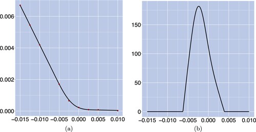
In figure 1, we illustrate the performance of the smoothing approach from two perspectives, the fit of market prices and the behaviour of the probability density. Figure 1(a) presents the interpolated prices and the market quoted prices for the caplet products of interest, $\mathrm{C}\mathrm{p}\mathrm{l}(0,6M,1Y)$. It can be observed that all market quotations are in line with the smoothed price curve, indicating that the interpolation technique is performing well as an accurate caplet valuation tool. Figure 1(b) shows that the market-implied density is non-negative and is positive in the range from approximately −0.7% to 0.3%. This indicates that the 6-month forward rate in 6 months is distributed in a quite narrow range and the probability of the potential value is the highest around −0.22% which is consistent with the level of the current forward rate. This illustrates the property that the expectation under the corresponding forward measure of the future forward rate matches the current forward rate.

Figure 1. Interpolated caplet prices and market-implied probability density under ${\mathbb{Q}}^S$ constructed based on the cap market data (quoted in normal volatility) on March 31, 2016. Panel (a) gives the market caplet prices (dots) computed by the Bachelier formula alongside with interpolated price curve obtained by the no-arbitrage cubic spline smoothing technique. Panel (b) provides the $L(6M,1Y)$ forward rate density implied from the interpolated caplet prices using equation (25(25) $\begin{array}{r}{f}_{L(T,S)|{\mathcal{F}}_t}^S\left(K\right)=\frac{\frac{{\mathrm{\partial }}^2}{\mathrm{\partial }{K}^2}{\mathrm{C}\mathrm{p}\mathrm{l}}_t(T,S,K)}{\mathrm{\Delta }{P}_t\left(S\right)}.\end{array}$(25) ). (a) Interpolated price curve and (b) implied density of $L(6M,1Y)$.

4.2. Calibration results for the implied-volatility curve

Equation (23(23) $\begin{array}{rl}{\mathrm{C}\mathrm{p}\mathrm{l}}_t(T,S,K)& =M_t\mathbb{E}\left[\frac{\left(L\right(T,S)-K{)}^{+}\mathrm{\Delta }}{M_S}|{\mathcal{F}}_t\right]\\ & =P_t\left(S\right){\mathbb{E}}^S\left[\left(L\right(T,S)-K{)}^{+}\mathrm{\Delta }|{\mathcal{F}}_t\right]\\ & =\mathrm{\Delta }{P}_t\left(S\right){\int }_K^{+\mathrm{\infty }}(v-K)f_{L(T,S)|{\mathcal{F}}_t}^S\left(v\right)\mathrm{d}v,\end{array}$(23) ) provides the model-implied caplet prices. The corresponding caplet volatilities, obtained via the Bachelier formula, can thus be compared with those extracted from market quotes as explained in section 3.1. The model is then calibrated according to equation (24(24) $\begin{array}{r}{\mathrm{\Psi }}^{z^{\ast }}:=\arg \underset{{\mathrm{\Psi }}^z}{min}\frac{1}{n}\sum _{i=1}^n{({\sigma }_i^M-{\sigma }_i^z)}^2\end{array}$(24) ). We provide the calibration performance on the first available date from our sample as an illustration.

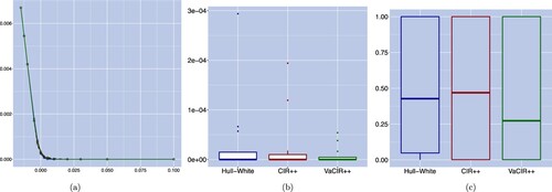
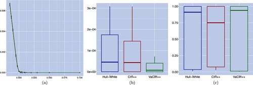
We plot in figure 2 the modelled implied volatilities, with associated squared errors in basis points and relative errors, using the parameters calibrated based on fitting the market-implied volatilities. Figure 2(a) shows the implied-volatility curves for each of the three calibrated models as well as the implied volatilities extracted from stripped market quotes, which serve here as calibration target. We observe that the CIR++ and the VaCIR++ models capture quite well the in-/at-the-money caplet volatilities but fail to capture accurately the data of the deep out-of-the-money products. The Hull–White model provides the worst fit as the modelled curve deviates from the market one for all products. Furthermore, the box plots of the associated squared and relative errors, displayed in figures 2(b,c) respectively, provide further details on the relative performance of the three models considered. The Hull–White model has the largest median value and dispersion for both the squared and relative errors while the error distribution of the VaCIR++ model is close to the CIR++ one but exhibits a slightly lower median value (squared errors) and less dispersion (relative errors).

Figure 2. Implied-volatility curves with associated squared errors (in bps) and relative volatility errors on March 31, 2016, where the models are calibrated on the criteria of implied volatility error minimization. Panel (a) shows the implied-volatility curves with respect to the strike for the market (dashed), Hull–White (□), CIR++ ($\mathrm{△}$) and VaCIR++ (⋄) models. Panel (b) and Panel (c) provide respectively the box plots of the associated squared and relative errors for the three candidate models. (a) Implied-volatility curve; (b) implied vol squared error and (c) implied vol relative error.

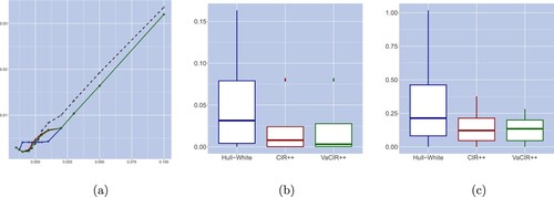
Figure 3 shows the same results as figure 2 but expressed in terms of prices rather than volatilities. It can be observed that all three considered models provide a close fit to the market price curve. When comparing between models, the inferior performance of the Hull–White model is further confirmed by pricing accuracy. In particular, the Hull–White model has the highest value in terms of squared errors and comparable relative errors to the CIR++ model. The VaCIR++ model provides the best performance in terms of both the squared and relative pricing errors. Not surprisingly, figure 3(a) indicates that a small implied volatility error for the in/at the money caplets can lead to a sizable discrepancy in prices while the out of the money caplets are subject to large differences in volatility but have almost indistinguishable price curves. This observation highlights the drawbacks of the calibration approaches fitting the implied volatilities or caplet prices. More specifically, the far out of the money options tend to have extremely low prices but rather high implied volatilities. Therefore, putting equal weight on the error of those products in the calibration target could sacrifice the accuracy in modelling the exact prices and volatilities for the at/in the money products. Thus a weighting scheme should be incorporated such that the information in such options would be substantially discounted. However, this approach would still be essentially focusing on a subset of products and would likely result in a poor overall fit.

Figure 3. Caplet price curves with corresponding squared errors (in bps) and relative pricing errors on March 31, 2016, where models are calibrated on the criteria of implied volatility error minimization. Panel (a) displays the market and modelled caplet prices with respect to the strike for the market (dashed), Hull–White (□), CIR++ ($\mathrm{△}$) and VaCIR++ (⋄) models. Panel (b) and panel (c) provide respectively the box plots of the corresponding squared errors and relative errors for the three candidate models. (a) Caplet price curve, (b) price squared error and (c) price relative error.

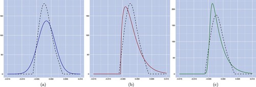
We further investigate the distribution of the forward rate under the three considered models compared to the market-implied one. Figure 4 displays respectively the density curves for the Hull–White, the CIR++ and the VaCIR++ models against the market-implied one. We observe that in general, the three models fail to match the market-implied forward rate density especially around the centre of the distribution and in the right tail. In particular, it can be observed from figure 4(a) that the forward rate distribution under the Hull–White model is symmetric and has a lower peak than the market-implied one. As shown in figures 4(b,c), the density under the CIR++ and VaCIR++ models provides a close fit on the left-hand side of the distribution but not in the centre or in the right tail. This observation suggests that the calibration approach focusing on a few implied volatility data points does not guarantee a match of the entire forward rate distribution.

Figure 4. Density curves of the forward rate $L(6M,1Y)$ on March 31, 2016, where models are calibrated on the criteria of implied volatility error minimization. Panel (a), panel (b) and panel (c) exhibit the market-implied forward density curve and the modelled forward density curves (dashed lines) and under the Hull–White, the CIR++ and VaCIR++ models, respectively (solid lines). (a) Hull–White model, (b) CIR++ model and (c) VaCIR++ model.

4.3. Calibration results for the forward rate density

Equipped with the smoothed caplet price curve computed over a fine grid of strikes, we now turn to the estimation of the market-implied forward rate distribution according to equation (25(25) $\begin{array}{r}{f}_{L(T,S)|{\mathcal{F}}_t}^S\left(K\right)=\frac{\frac{{\mathrm{\partial }}^2}{\mathrm{\partial }{K}^2}{\mathrm{C}\mathrm{p}\mathrm{l}}_t(T,S,K)}{\mathrm{\Delta }{P}_t\left(S\right)}.\end{array}$(25) ). We then calibrate the three considered models according to algorithm 2 to closely match the market-implied density by minimizing the discrepancy (measured by JS divergence) between the model-implied and market-implied curves. As in the previous section, we take the first available date from our sample and investigate the distribution of the forward rate under the three candidates compared to the market-implied one.

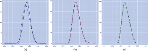
We plot in figure 5 the density curves obtained by calibrating each of the three models (solid lines). Figure 5(a) shows that the calibrated density under the Hull–White model has a right-shifted distribution and is more symmetric, compared to the market-implied one. Furthermore, it provides a closer fit to the market-implied density on the right-hand side but deviates significantly on the left-hand side. In addition, we plot in figure 5(b) the density under the CIR++ model, we observe that it has a slightly higher peak than the market-implied density but it captures quite well the skewness exhibited by the market density. In particular, it provides an almost perfect fit on the left-hand side although it fails to match the right-hand tail in the forward rate distribution. Lastly, the calibrated density obtained from the VaCIR++ model is displayed in figure 5(c), and we conclude that the combined model matches well both tails and captures the overall market-implied density curve better than the Hull–White and CIR++ models. Furthermore, the superior performance of the VaCIR++ is confirmed by the significantly lower JS divergence value on this calibration date compared to the alternative models (see figure 9). This observation is consistent with the argument that the VaCIR++ model will perform at least as well as its underlying component processes and it will be inclined to place a higher weight on the component process exhibiting better calibration performance, the CIR++ process in this case. It is worth noting that the model-implied densities obtained from the density matching calibration approach provide a tighter fit to the market-implied one compared to the results displayed in figure 4 which are based on the implied volatility MSE criterion.

Figure 5. Density curves of the forward rate $L(6M,1Y)$ on March 31, 2016, where models are calibrated on the criteria of JS divergence minimization. Panel (a), panel (b) and panel (c) exhibit the market-implied forward density curve (dashed lines) and the modelled forward density curves under the Hull–White, CIR++ and VaCIR++ models, respectively (solid lines). (a) Hull–White model, (b) CIR++ model and (c) VaCIR++ model.

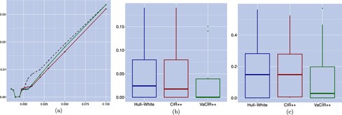
We further illustrate in figure 6 the pricing accuracy of the three models using the calibrated parameters based on density matching. Figure 6(a) compares the model-implied caplet prices to the market data.¹² It can be concluded that all three models are able to provide a quite accurate valuation for the caplet products. The squared and relative pricing errors under the three models are plotted in figures 6(b,c). The bar in the boxplots represents the median of the errors while the lower and upper bounds of each box represent the first and third quartiles respectively. We observe that the VaCIR++ model provides the lowest pricing errors while the Hull–White and CIR++ models have comparable pricing accuracy. Additionally, we note that high absolute pricing accuracy does not necessarily translate to better performance in terms of relative pricing errors as close to zero prices might lead to high relative pricing errors. Furthermore, high pricing accuracy indicates that the better density fit obtained when adopting the JS divergence calibration technique instead of the price or implied volatility MSE criterion does not come at the cost of larger pricing errors.

Figure 6. Caplet price curves with corresponding mean squared errors (in bps) and relative pricing errors on March 31, 2016, where models are calibrated on the criteria of JS divergence minimization. Panel (a) displays the market and modelled caplet prices with respect to the strike for the market (dashed), Hull–White (□), CIR++ ($\mathrm{△}$) and VaCIR++ (⋄) models. Panel (b) and panel (c) provide respectively the box plots of the corresponding mean squared errors and relative errors for the three candidate models. (a) Caplet price curve, (b) price squared error and (c) price relative error.

In addition, we assess in figure 7 the performance of the three models in terms of how close their implied-volatility curves, arising from minimizing the JS divergence, are to the market-based implied-volatility curve. Figure 7(a) shows that there are visible discrepancies between the implied volatilities under the CIR++ model and the market ones for caplet products with strikes between 0% and 1%. Outside that range, the VaCIR++ model has superior matching performance of the implied-volatility curve. Furthermore, we note that the calibration focused on density matching also provides convincing fitting performance in terms of implied volatility errors. Therefore, we conclude that the density matching approach provides a more robust way of calibrating interest rate models to fixed income derivative data since it has superior performance in capturing the entire forward distribution, high pricing accuracy and comparable fitting quality in terms of matching implied-volatility curves.¹³

Figure 7. Implied-volatility curves with associated squared and relative volatility errors on March 31, 2016, where the models are calibrated on the criteria of JS divergence minimization. Panel (a) contains the implied-volatility curves with respect to the strike for the market (dashed), Hull–White (□), CIR++ ($\mathrm{△}$) and VaCIR++ (⋄) models. Panel (b) and Panel (c) provide respectively the box plots of the associated squared errors and relative errors for the three candidate models. (a) Implied-volatility curve; (b) implied vol squared error and (c) implied vol relative error.

Thus far, our analysis focused on benchmarking our two-factor VaCIR++ model with the two components, namely the one-factor Hull–White and CIR++ models. Therefore, we also include additional two-factor models in the comparison to capture the added flexibility associated with the use of a two-factor model. We opt for the G2++ model which is a two-factor Gaussian model introducing correlation between its two Brownian motions through an additional parameter ρ. Additionally, we consider the CIR2++ model whose underlying factors are two independent CIR processes.¹⁴${}^{,}$¹⁵ We plot in figure 8 the density curves obtained by calibrating the G2++ and CIR2++ models (solid lines) to the market data. Figure 8(a) shows that the calibrated density under the G2++ model is almost identical to the density obtained from a Hull–White model presented in figure 5(a), namely it has a right-shifted distribution and is more symmetric, compared to the market-implied one. It is worth noting that the G2++ model provides indistinguishable performance to its one-factor counterpart ( Hull–White) which indicates that the additional flexibility from the two-factor model leads to limited added value for our application.¹⁶ In addition, the calibrated density obtained from the CIR2++ model is displayed in figure 8(b), and we conclude that it provides a similar but closer fit to the market-implied density compared to its one-factor counterpart. Comparing both figures to figure 8(c), the VaCIR++ model provides a better overall fit to the market-implied density curve than the two-factor benchmarks. The superior performance of the VaCIR++ is confirmed by the significantly lower JS divergence value on this calibration date (see figure 9).

Figure 8. Density curves of the forward rate $L(6M,1Y)$ on March 31, 2016, where models are calibrated on the criteria of JS divergence minimization. Panel (a), Panel (b) and panel (c) exhibit the market-implied forward density curve and the modelled forward density curves (dashed lines) and under the G2++, CIR2++ and VaCIR++ models, respectively (solid lines). (a) The G2++ model; (b) the CIR2++ model and (c) VaCIR++ model.

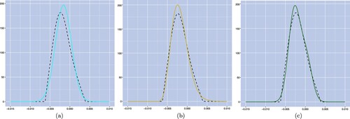
Figure 9. Evolution over time of the JS divergence resulting from the density matching calibration under the Hull–White (□, dark blue), CIR++ ($\mathrm{△}$, red), G2++ (♦, light blue), CIR2++ (+, yellow) and VaCIR++ ($◊$, green) models.

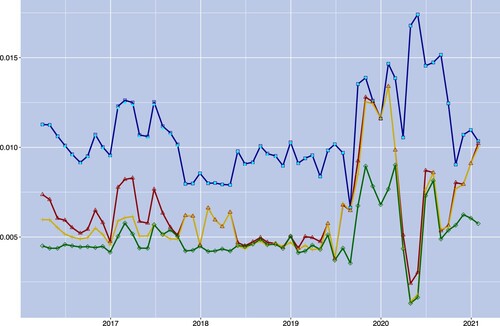
We further investigate how model performance—measured in terms of matching the market-implied density curve—evolves over time. To this end, the five models considered are calibrated on a monthly basis and we report in figure 9 the JS divergence for each of them. When comparing the VaCIR++ model to its two one-factor component models, the best-in-class property of VaCIR++ is preserved through time. In particular, it always has the lowest JS divergence, indicating closest matching to the market-implied density curve. Also, we can observe that the CIR++ model exhibits better performance than the Hull–White model which makes the CIR++ model an attractive candidate as a single-factor model—with the shift providing some flexibility to deal with negative rates. Additionally, we observe that the performance of the G2++ and Hull–White models in terms of matching the market-implied forward rate density are essentially indistinguishable. See the light blue marks (G2++ model) in figure 9 which are almost perfectly aligned with the dark blue curve (Hull–White model). In fact, the estimated parameter ρ under the G2++ model is rather close to −1 over the whole sample period. In this case, the G2++ model degenerates into a one-factor short-rate process. This observation is consistent with the results of the empirical application presented in chapter 4 of Brigo and Mercurio (2007). Furthermore, the VaCIR++ model outperforms the CIR2++ benchmark on most calibration dates with only a few exceptions where the CIR2++ model has a slightly lower JS divergence. Lastly, we can observe that the added flexibility of the CIR2++ provides superior performance over the one-factor CIR++, in particular over the first part of the sample. To summarize, the VaCIR++ model is more appealing both theoretically—allowing for negative values, skewness, and no strict lower bound—and empirically as it enhances the fitting performance compared to the four benchmark models and improves calibration stability over time.

Based on the density obtained, we characterize the variation of the implied conditional moments of the forward rate $L(T,S)$ (under the S-forward measure) over time.¹⁷ In this manner, we compute the first four conditional moments for the 6-month forward rate in 6 months over the whole sample period and investigate how well each of the five competing models can match the market-implied moments (figure 10). It can be observed from figure 10(a) that the five models accurately track the market-implied mean overall—with the Hull-White, CIR++ and G2++ models exhibiting slight discrepancies in the first 2 years of the sample period. Figure 10(b) shows that the Gaussian models (Hull–White and G2++) have the worst performance in terms of tracking the market-implied standard deviation while the CIR2++ model provides the best fit overall. For the skewness, illustrated in figure 10(c), we observe that the conditional skewness of the forward rate distribution under the Hull–White and G2++ models is almost zero indicating that these two models are unable to capture the skewness featured in the data. The conditional skewness under the CIR++ and CIR2++ is positive, though higher than the market-implied one in general. The conditional skewness under the VaCIR++ model is the closest to the market-implied one, except for a few months in 2018 and 2019 where the model performance is comparable to the CIR++ and CIR2++ models. Lastly, figure 10(d) illustrates that the excess kurtosis under the Hull–White and G2++ models is close to zero while the densities implied by the CIR++ and CIR2++ models always exhibit positive excess kurtosis. In both cases, the model-implied excess kurtosis is overall higher than the market-implied one. The excess kurtosis implied by the VaCIR++ model provides, however, a better tracking of the market-implied one, especially in the first part of the sample. The jumps observed in the conditional skewness and excess kurtosis for the VaCIR++ model might be caused by local minima in the optimization and warrant further investigation. We also note that the CIR++ and VaCIR++ models have similar levels of JS divergence during those months but this does not necessarily imply that the two models have similar densities or conditional moments. Indeed, the two model-implied distributions could be equally similar to the market one while being noticeably different from each other.

Figure 10. Time series of the $L(6M,1Y)$ conditional moments for the market (°) and for the Hull–White (□, dark blue), CIR++ ($\mathrm{△}$, red), G2++ (♦, light blue), CIR2++ (+, yellow) and VaCIR++ ($◊$, green) models. (a) Conditional mean; (b) conditional standard deviation; (c) conditional skewness and (d) conditional excess kurtosis.

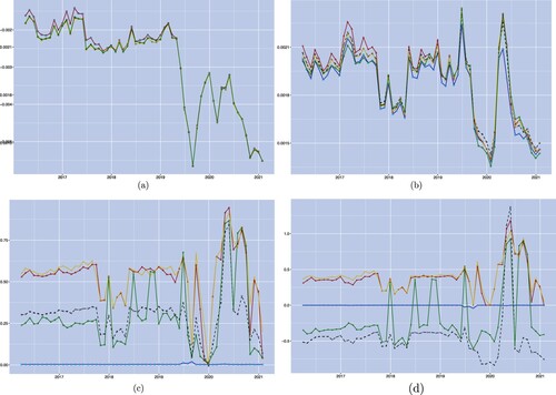
Finally, focusing on the forward rate density and its conditional moments also provides us with relevant market insights for risk management and hedging applications. As shown in figure 10(a,b), the mean and standard deviation of the future forward rate are stable at the beginning of the sample period. In particular, for the level of the mean, a significant downturn followed by an increasing trend is observed during 2019 while the period from 2020 to 2021 is dominated by a downward shift. The standard deviation, on the other hand, exhibits a significant upward movement followed by a short decline during 2019 and is then strongly trending upward during the period from 2020 to 2021. This more volatile evolution of interest rates during the COVID-19 period is likely due to the increased uncertainty in financial markets and concerns for funding conditions resulting from the crisis. Furthermore, figure 10(c) shows that the conditional skewness is generally positive with a sharp increase at the onset of the COVID-19 crisis followed by a steady decrease over the rest of the sample period. We observe a similar behaviour in figure 10(d) for the excess kurtosis during COVID. Overall, excess kurtosis is negative over our sample, indicating a lower tail-thickness compared to a Gaussian distribution.

5. Conclusion

We propose a simple asymmetric short-rate model that does not display a strict lower bound and is well suited to capture the salient features of the negative interest rate environment. Our two-factor model, called the VaCIR++ model, combines the advantages of the Hull–White model (no strict lower bound) and the CIR++ model (positive skewness) while maintaining analytical tractability. Our framework delivers semi-analytical expressions for the forward rate density and caplet pricing which allows us to tackle the challenges encountered by standard benchmark models for the modelling and pricing of interest rate derivatives in a negative interest rate environment.

In addition, we introduce a new calibration procedure based on density matching which alleviates the drawbacks inherent to standard model calibration procedures based on prices or volatilities mean squared error. Precisely, the model is calibrated such that the model-implied density is the closest to the market-implied one in terms of Jensen–Shannon divergence. While in this context, we match the forward rate densities computed under the forward measure, our approach can be broadly applied to other settings where the interest lies in closely matching a chosen target density.

Finally, we illustrate the benefits of our framework in a financial application featuring a time series of caplets whose prices are retrieved by stripping cap implied volatilities. We provide a comparative study of calibration performance in the period of negative interest rates under two calibration criteria—the volatility mean squared error minimization and our proposed density matching approach based on the minimization of the Jensen–Shannon divergence. We note the outperformance of our model relative to the Hull–White and CIR++ models. Moreover, the calibration procedure based on the Jensen–Shannon divergence significantly enhances the matching of the forward densities while preserving high pricing accuracy and comparable fitting quality for implied-volatility curves.

Our work can be extended in several ways. First, our modelling framework can be extended to consider simultaneously multiple forward rate maturities and contract expiry lengths. This would allow us to explore the benefits of extracting information relevant for model calibration using liquid products and apply this calibration to the pricing of less liquid products within a consistent framework. Second, the strength of the economic recovery following the COVID-19 crisis, combined with the escalation of the conflict between Russia and Ukraine, led to a strong revival of inflationary pressures. As major central banks reacted to these events by raising their policy rates, it would be interesting to evaluate how our proposed model and calibration approach perform in a period where interest rates revert back to higher levels.

Acknowledgments

The authors are grateful to Damiano Brigo and Donatien Hainaut for insightful comments on earlier versions of this manuscript.

Disclosure statement

No potential conflict of interest was reported by the authors.

Additional information

Funding

This work was supported by the Belgian Federal Science Policy Office [ARC grant number 18-23/089].

Notes

1 While we focus the exposition on the univariate case, multi-dimensional jump-diffusion models can be considered.

2 In these expressions, the constraints on the parameters are as follows: ${\kappa }_1,{\sigma }_1,y_0,{\kappa }_2,{\theta }_2,{\sigma }_2$ are positive constants and $2{\kappa }_2{\theta }_2>{\sigma }_2^2$ (Feller condition).

3 They are recalled in appendix 1 for $z\in \{x,y$}.

4 Of course, with the deterministic shift extension, the expression for forward rates should also be adjusted for the shift term, which can be rewritten as $F_t^{z^{\varphi }}(T,S)=\frac{1}{\mathrm{\Delta }}({\mathrm{e}}^{-{\int }_T^S{\phi }^z\left(s\right)ds}\frac{P_t^z\left(T\right)}{P_t^z\left(S\right)}-1),z\in \{x,y,r\}$.

5 Since x and y are independent, $L^x(T,S)|{\mathcal{F}}_t$ is equivalent to $L^x(T,S)|x_t$, $L^y(T,S)|{\mathcal{F}}_t$ is equivalent to $L^y(T,S)|y_t$ and $L^r(T,S)|{\mathcal{F}}_t$ is equivalent to $L^r(T,S)|(x_t,y_t)$.

6 See Breeden and Litzenberger (1978) for a seminal contribution and Brigo and Mercurio (2007) for a textbook treatment in the context of caplet pricing.

7 A detailed outline of this procedure is provided in appendix 2.

8 The KL divergence is not a distance because the triangular inequality may fail to hold. See Basseville (2013) for a review of statistical applications using divergence measures.

9 We opt for the KL divergence compared to the $L^2$ metric for density calibration as this measure does not properly scale with the distribution—exacerbating (resp. minimizing) discrepancies between densities in high (resp. low) density regions—which would impact calibration accuracy. Other choices, such as e.g. the Hellinger distance used in Tavin (2012), could be entertained and are left for future research.

10 Volatility modelling and market-implied density are only needed under the calibration method using JS divergence. The calibration method minimizing the mean squared error is based on the implied volatility data directly obtained from caplet stripping.

11 The discount curve and all the related interest derivatives are based on the 6-month EURIBOR rates for consistency.

12 We note that the market prices are recovered by computing the risk-neutral expectation of the discounted payoffs using the market-implied density as the resulting prices are more comparable with the model-implied ones. This is due to the fact that the prices consistent with the market-implied density, obtained as a by-product of the no-arbitrage volatility curve smoothing, might slightly differ from the actual market prices, which are not necessarily free from arbitrage opportunities.

13 Note that, although our approach takes into account the entire forward rate distribution in the calibration, it does not provide at the moment an explicit way to assign different weights on the calibration products to reflect their different degrees of data reliability (moneyness or liquidity). This is indeed an interesting question, which would increase the practical relevance of our approach. However, we propose to keep this extension for future work. We thank one of the anonymous referees for pointing this out.

14 The interested reader is referred to chapter 4 of Brigo and Mercurio (2007) for more details on the G2++ and CIR2++ models.

15 In terms of model complexity, the one-factor Hull–White and CIR++ models have each four parameters while the G2++ model is parameterized with six parameters. The CIR2++ and VaCIR++ models have eight parameters to estimate.

16 Although the two-factor G2++ model has limited contribution in our application compared to the one-factor Hull–White model, it might lead to improved performance in empirical applications where the correlation between forward rates plays an essential role in the calibration; e.g. for swaption contracts.

17 The market- and model-implied conditional moments are computed numerically using the corresponding forward rate density.

Appendices

Appendix 1.

Pricing formula for existing framework

We provide below the $A^z$ and $B^z$ functions in equation (3(3) $\begin{array}{r}\mathrm{d}{z}_t=(a+b{z}_t)\mathrm{d}t+\sqrt{c+d{z}_t}\mathrm{d}{W}_t,z_0>-c/d,\mathrm{\forall }d>0,\end{array}$(3) ) for $z\in \{x,y,y^{\varphi }\}$. For conciseness, we omit the subscript in the $\kappa ,\theta ,\sigma$ parameters.

For the Vasicek model specified in equation (1(1) $\begin{array}{rl}\mathrm{d}{x}_t& ={\kappa }_1({\theta }_1-x_t)\mathrm{d}t+{\sigma }_1\mathrm{d}{W}_t^x,x_0\in \mathbb{R},\end{array}$(1) ), we have $\begin{array}{rl}{A}^x\left(\tau \right)& =\exp \left\{(\theta -\frac{{\sigma }^2}{2k^2})\right[B\left(\tau \right)-\tau ]-\frac{{\sigma }^2}{4k}{B}^x(\tau {)}^2\},\\ B^x\left(\tau \right)& =\frac{1}{k}[1-{\mathrm{e}}^{-k\tau }].\end{array}$ For the CIR model specified in equation (2(2) $\begin{array}{rl}\mathrm{d}{y}_t& ={\kappa }_2({\theta }_2-y_t)\mathrm{d}t+{\sigma }_2\sqrt{y_t}\mathrm{d}{W}_t^y,y_0\in {\mathbb{R}}_0^{+}.\end{array}$(2) ), $\begin{array}{rl}{A}^y\left(\tau \right)& ={\left[\frac{2h\exp \left\{\right(k+h\left)\tau /2\right\}}{2h+(k+h)(\exp \{h\tau \}-1)}\right]}^{2k\theta /{\sigma }^2},\\ B^y\left(\tau \right)& =\frac{2(\exp \{h\tau \}-1)}{2h+(k+h)(\exp \{h\tau \}-1)}.\end{array}$ where $h=\sqrt{k^2+2{\sigma }^2}$.

The shifted CIR model is a special case of a general model proposed in Brigo and Mercurio (2001). It can be shown that $A^{y^{\varphi }}\left(\tau \right)={\mathrm{e}}^{-\varphi \tau }{A}^y\left(\tau \right),B^{y^{\varphi }}\left(\tau \right)=B^y\left(\tau \right).$

Appendix 2.

Arbitrage-free smoothing of the volatility curve

Following the notations in Fengler (2009), assume that we observe the caplet prices $\mathbf{y}=(y_1,\dots ,y_n)$ at the strikes $a=u_0,\dots ,u_{n+1}=b$, and the function g represents the natural cubic spline function. For the value and second derivative representation, we set $g_i=g\left(u_i\right)$ and ${\gamma }_i=g^{\mathrm{\prime }\mathrm{\prime }}\left(u_i\right),$ for $i=1,\dots ,n.$ Furthermore, we define $\mathbf{g}=(g_1,\dots ,g_n{)}^{\mathrm{\top }}$ and $\mathit{\gamma }=({\gamma }_2,\dots ,{\gamma }_{n-1}{)}^{\mathrm{\top }}$. By definition, ${\gamma }_1={\gamma }_n=0$.

We formulate the sufficient and necessary conditions to ensure a valid cubic spline using the two matrices $\mathbf{Q}$ and $\mathbf{R}$ defined below. Let $h_i=u_{i+1}-u_i$ for $i=1,\dots ,n-1,$ and the elements $q_{i,j},$ of matrix $\mathbf{Q}$, for $i=1,\dots ,n$ and $j=2,\dots ,n-1$, are given by $q_{j-1,j}=h_{j-1}^{-1},q_{j,j}=-h_{j-1}^{-1}-h_j^{-1}\mathrm{a}\mathrm{n}\mathrm{d}{q}_{j+1,j}=h_j^{-1},$ for $j=2,\dots ,n-1$ and $q_{i,j}=0$ for $|i-j|\ge 2$.

The matrix $\mathbf{R}$ is symmetric and its elements $r_{i,j}$, for $i,j=2,\dots ,n-1,$, are defined by $\begin{array}{rl}{r}_{i,i}& =\frac{1}{3}(h_{i-1}+h_i),\mathrm{f}\mathrm{o}\mathrm{r}i=2,\dots ,n-1\\ r_{i,i+1}& =r_{i+1,i}=\frac{1}{6}{h}_i,\mathrm{f}\mathrm{o}\mathrm{r}i=2,\dots ,n-2\\ r_{i,j}& =0,\mathrm{f}\mathrm{o}\mathrm{r}|i-j|\ge 2\end{array}$ Furthermore, we formulate the spline smoothing problem as a quadratic minimization program. Define vector $\mathbf{y}=(w_1{y}_1,\dots ,w_n{y}_n,0,\dots ,0{)}^{\mathrm{\top }},$ where the $w_i$ are strictly positive weights and vector $\mathbf{x}=({\mathbf{g}}^{\mathrm{\top }},{\mathit{\gamma }}^{\mathrm{\top }}{)}^{\mathrm{\top }}$. Furthermore, define the matrices, $\mathbf{A}=(\mathbf{Q},-{\mathbf{R}}^{\mathrm{\top }})$ and $\mathbf{B}=\left(\begin{array}{cc}{\mathbf{W}}_n& 0\\ 0& \lambda \mathbf{R}\end{array}\right)$ where ${\mathbf{W}}_n=\mathrm{diag}(w_1,\dots ,w_n)$. The smoothing algorithm of the volatility curve is summarized below.

1. Estimate the volatility curve via an initial interpolation of caplet prices with respect to the moneyness, which is defined as the strikes in excess to the forward rate.

2. Obtain the implied-volatility curve using the spline smoothing technique under no-arbitrage constraints by solving the quadratic program formulated as follows: $\begin{array}{rl}& \underset{\mathbf{x}}{min}-{\mathbf{y}}^{\mathrm{\top }}\mathbf{x}+\frac{1}{2}{\mathbf{x}}^{\mathrm{\top }}\mathbf{B}\mathbf{x},\\ & \mathrm{s}\mathrm{u}\mathrm{b}\mathrm{j}\mathrm{e}\mathrm{c}\mathrm{t}\mathrm{t}\mathrm{o}{\mathbf{A}}^{\mathrm{\top }}\mathbf{x}=0,\\ & {\gamma }_i\ge 0,\\ & \frac{g_2-g_1}{h_1}-\frac{h_1}{6}{\gamma }_2\ge P_t\left(S\right)(S-T),\\ & -\frac{g_n-g_{n-1}}{h_{n-1}}-\frac{h_{n-1}}{6}{\gamma }_{n-1}\ge 0.\end{array}$

Appendix 3.

Correlation between two factors

A.1. Introduce correlation within the affine framework

Assume short rate is defined as $r_t=X_t^1+X_t^2$ and the two factors in the model $X_t=(X_t^1,X_t^2)$ are described as the following system of SDEs under the risk-neutral Q -measure: $\begin{array}{rl}\left(\begin{array}{c}\mathrm{d}{X}_t^1\\ \mathrm{d}{X}_t^2\end{array}\right)& =\left(\begin{array}{cc}{\kappa }_1& 0\\ 0& {\kappa }_2\end{array}\right)[\left(\begin{array}{c}{\theta }_1\\ {\theta }_2\end{array}\right)-\left(\begin{array}{c}{X}_t^1\\ X_t^2\end{array}\right)]\mathrm{d}t\\ & +\left(\begin{array}{cc}{\sigma }_{11}& 0\\ {\sigma }_{21}& {\sigma }_{22}\end{array}\right)\left(\begin{array}{cc}\sqrt{X_t^1}& 0\\ 0& 1\end{array}\right)\left(\begin{array}{c}\mathrm{d}{W}_t^1\\ \mathrm{d}{W}_t^2\end{array}\right),\end{array}$ which is equivalent to $\begin{array}{rl}\left(\begin{array}{c}\mathrm{d}{X}_t^1\\ \mathrm{d}{X}_t^2\end{array}\right)& =\left(\begin{array}{cc}{\kappa }_1& 0\\ 0& {\kappa }_2\end{array}\right)[\left(\begin{array}{c}{\theta }_1\\ {\theta }_2\end{array}\right)-\left(\begin{array}{c}{X}_t^1\\ X_t^2\end{array}\right)]\mathrm{d}t+\\ & \left(\begin{array}{cc}{\sigma }_{11}\sqrt{X_t^1}& 0\\ {\sigma }_{21}\sqrt{X_t^1}& {\sigma }_{22}\end{array}\right)\left(\begin{array}{c}\mathrm{d}{W}_t^1\\ \mathrm{d}{W}_t^2\end{array}\right).\end{array}$ We can rewrite it as $\begin{array}{rl}\mathrm{d}{X}_t^1& ={\kappa }_1({\theta }_1-X_t^1)\mathrm{d}t+{\sigma }_{11}\sqrt{X_t^1}\mathrm{d}{W}_t^1,\\ \mathrm{d}{X}_t^2& ={\kappa }_2({\theta }_2-X_t^2)\mathrm{d}t+{\sigma }_{21}\sqrt{X_t^1}\mathrm{d}{W}_t^1+{\sigma }_{22}\mathrm{d}{W}_t^2.\end{array}$ Here, the correlation between the two factors $X_t^1,X_t^2$ is introduced by ${\sigma }_{21}$. If we set ${\sigma }_{21}=0$, this framework reduces to the case where we have two independent processes with $X_t^1$ being a CIR process and $X_t^2$ being a Vasicek process. In addition, this belongs to the Affine framework given that $\begin{array}{rl}\mathrm{\Sigma }{\mathrm{\Sigma }}^{\mathrm{\prime }}& =\left(\begin{array}{cc}{\sigma }_{11}\sqrt{X_t^1}& 0\\ {\sigma }_{21}\sqrt{X_t^1}& {\sigma }_{22}\end{array}\right)\left(\begin{array}{cc}{\sigma }_{11}\sqrt{X_t^1}& {\sigma }_{21}\sqrt{X_t^1}\\ 0& {\sigma }_{22}\end{array}\right)\\ & =\left(\begin{array}{cc}{\sigma }_{11}^2{X}_t^1& {\sigma }_{11}{\sigma }_{21}{X}_t^1\\ {\sigma }_{11}{\sigma }_{21}{X}_t^1& {\sigma }_{21}^2{X}_t^1+{\sigma }_{22}^2\end{array}\right).\end{array}$ The zero coupon bond price is defined as $\begin{array}{rl}{P}_t^r\left(T\right)& =\exp \left(B\right(T-t{)}^{\mathrm{\prime }}{X}_t+A(T-t))\\ & =\exp \left(B^1\right(T-t)X_t^1+B^2(T-t)X_t^2+A(T-t\left)\right).\end{array}$ For the factor loadings in the zero-coupon bond prices, A and B are the solutions to $\begin{array}{rl}\frac{\mathrm{d}{B}^1(t,T)}{\mathrm{d}t}& =1+{\kappa }_2{B}^1(t,T)-\frac{1}{2}{\left({\sigma }_{21}{B}^2\right(t,T)+{\sigma }_{11}{B}^1(t,T\left)\right)}^2,\\ \frac{\mathrm{d}{B}^2(t,T)}{\mathrm{d}t}& =1+{\kappa }_1{B}^2(t,T),\\ \frac{\mathrm{d}A(t,T)}{\mathrm{d}t}& =-{\kappa }_1{\theta }_1{B}^1(t,T)-{\kappa }_2{\theta }_2{B}^2(t,T)-\frac{1}{2}{\sigma }_{22}^2{B}^2(t,T{)}^2.\end{array}$ The solutions to $B(t,T)$ are formulated as $\begin{array}{rl}{B}^1(t,T)& =B^1(T-t)=-\frac{1}{{\kappa }_1}[1-{\mathrm{e}}^{-{\kappa }_1(T-t)}],\\ B^2(t,T)& =B^2(T-t)\\ & =-\frac{(2-{\sigma }_{21}^2{B}^1(t,T{)}^2\left)\right(\exp \left\{\right(T-t\left)h\right\}-1)}{2h+(h+{\kappa }_2-{\sigma }_{21}{\sigma }_2{B}^1(t,T\left)\right)(\exp \{(T-t)h\}-1)},\\ h& =\sqrt{2{\sigma }_{21}{\kappa }_2{\sigma }_2{B}^1(T-t)-{\kappa }_2^2-2{\sigma }_2^2}.\end{array}$ and the solution to $A(t,T)$ can be obtained by integration.

A.2. Introduce correlation by correlated Brownian motions

Assume $W_t^1,W_t^2$ are independent Brownian motions, and the short rate $r_t=X_t^1+X_t^2$. $\begin{array}{rl}\left(\begin{array}{c}\mathrm{d}{X}_t^1\\ \mathrm{d}{X}_t^2\end{array}\right)& =\left(\begin{array}{cc}{\kappa }_1& 0\\ 0& {\kappa }_2\end{array}\right)[\left(\begin{array}{c}{\theta }_1\\ {\theta }_2\end{array}\right)-\left(\begin{array}{c}{X}_t^1\\ X_t^2\end{array}\right)]\mathrm{d}t\\ & +\left(\begin{array}{cc}{\sigma }_{11}\sqrt{X_t^1}& 0\\ \rho {\sigma }_{22}& \sqrt{1-{\rho }^2}{\sigma }_{22}\end{array}\right)\left(\begin{array}{c}\mathrm{d}{W}_t^1\\ \mathrm{d}{W}_t^2\end{array}\right),\end{array}$ We can rewrite it as $\begin{array}{rl}\mathrm{d}{X}_t^1& ={\kappa }_1({\theta }_1-X_t^1)\mathrm{d}t+{\sigma }_{11}\sqrt{X_t^1}\mathrm{d}{W}_t^1,\\ \mathrm{d}{X}_t^2& ={\kappa }_2({\theta }_2-X_t^2)\mathrm{d}t+\rho {\sigma }_{22}\mathrm{d}{W}_t^1+\sqrt{1-{\rho }^2}{\sigma }_{22}\mathrm{d}{W}_t^2\\ & ={\kappa }_2({\theta }_2-X_t^2)\mathrm{d}t+{\sigma }_{22}\mathrm{d}{W}_t^3,\end{array}$ where $W_3$ is a Brownian motion satisfying $corr(\mathrm{d}{W}_t^1,\mathrm{d}{W}_t^3)=\rho \mathrm{d}t$.

Here, ρ introduce a correlation between the CIR process and the Vasicek process by correlated Brownian motions. If we set $\rho =0$, this framework reduces to the case where we have two independent processes with $X_t^1$ being a CIR process and $X_t^2$ being a Vasicek process. When $\rho \ne 0$, this model is no longer affine since $\begin{array}{rl}\mathrm{\Sigma }{\mathrm{\Sigma }}^{\mathrm{\prime }}& =\left(\begin{array}{cc}{\sigma }_{11}\sqrt{X_t^1}& 0\\ \rho {\sigma }_{22}& \sqrt{1-{\rho }^2}{\sigma }_{22}\end{array}\right)\left(\begin{array}{cc}{\sigma }_{11}\sqrt{X_t^1}& \rho {\sigma }_{22}\\ 0& \sqrt{1-{\rho }^2}{\sigma }_{22}\end{array}\right)\\ & =\left(\begin{array}{cc}{\sigma }_{11}^2{X}_t^1& \rho {\sigma }_{11}{\sigma }_{22}\sqrt{X_t^1}\\ \rho {\sigma }_{11}{\sigma }_{22}\sqrt{X_t^1}& {\sigma }_{22}^2\end{array}\right),\end{array}$

Appendix 4.

Proof of proposition 1

Point (a) is obtained by combining equation (11(11) $\begin{array}{rl}{P}_t^r\left(T\right)& =P_t^x\left(T\right)P_t^y\left(T\right)\\ & =A^x(T-t)A^y(T-t){\mathrm{e}}^{-\left[B^x\right(T-t)x_t+B^y(T-t\left)y_t\right]}.\end{array}$(11) ) with equation (12(12) $\begin{array}{r}{F}_t^z(T,S)=\frac{1}{\mathrm{\Delta }}(\frac{P_t^z\left(T\right)}{P_t^z\left(S\right)}-1),z\in \{x,y,r\}.\end{array}$(12) ). For point (b), we have the dynamics of the zero-coupon bond price for $z\in \{x,y\}$ $\frac{\mathrm{d}{P}_t^z\left(T\right)}{P_t^z\left(T\right)}=z_t\mathrm{d}t+B^z(T-t){\sigma }_t^z\mathrm{d}{W}_t^z,0\le t\le T.$

Applying Ito's quotient rule, we have for $0\le t\le T<S$, $\begin{array}{rl}& \frac{\mathrm{d}\left(P_t^z\right(T\left)/P_t^z\right(S\left)\right)}{P_t^z\left(T\right)/P_t^z\left(S\right)}\\ & =\frac{\mathrm{d}{P}_t^z\left(T\right)}{P_t^z\left(T\right)}-\frac{\mathrm{d}{P}_t^z\left(S\right)}{P_t^z\left(S\right)}-\frac{\mathrm{d}{P}_t^z\left(T\right)}{P_t^z\left(T\right)}\frac{\mathrm{d}{P}_t^z\left(S\right)}{P_t^z\left(S\right)}+{\left(\frac{\mathrm{d}{P}_t^z\left(S\right)}{P_t^z\left(S\right)}\right)}^2\\ & ={\sigma }_t^z\left(B^z\right(T-t)-B^z(S-t\left)\right)(\mathrm{d}{W}_t^z-{\sigma }_t^z{B}^z(S-t\left)\mathrm{d}t\right).\end{array}$ Combining this expression with (12(12) $\begin{array}{r}{F}_t^z(T,S)=\frac{1}{\mathrm{\Delta }}(\frac{P_t^z\left(T\right)}{P_t^z\left(S\right)}-1),z\in \{x,y,r\}.\end{array}$(12) ), the dynamics of the forward rate become $\begin{array}{rl}\mathrm{d}{F}_t^z(T,S)& =\frac{1}{\mathrm{\Delta }}\mathrm{d}\left(P_t^z\right(T\left)/P_t^z\right(S\left)\right)\\ & =(\frac{1}{\mathrm{\Delta }}+F_t^z(T,S\left)\right){\sigma }_t^z\left(\right(B^z(S-t)-B^z(T-t))\\ & \times (-{\sigma }_t^z{B}^z(S-t)\mathrm{d}t+\mathrm{d}{W}_t^z)\\ & ={\sigma }^z(t,F_t^z(T,S\left)\right)(-{\zeta }_t^{z,S}\mathrm{d}t+\mathrm{d}{W}_t^z)\\ & ={\sigma }^z(t,F_t^z(T,S\left)\right)\mathrm{d}{W}_t^{z,S},\end{array}$ where (30) $\begin{array}{r}{\sigma }^z(t,v):={\sigma }_t^z[\frac{1}{\mathrm{\Delta }}+v]\left(\right(B^z(S-t)-B^z(T-t)).\end{array}$(30) Using equation (11(11) $\begin{array}{rl}{P}_t^r\left(T\right)& =P_t^x\left(T\right)P_t^y\left(T\right)\\ & =A^x(T-t)A^y(T-t){\mathrm{e}}^{-\left[B^x\right(T-t)x_t+B^y(T-t\left)y_t\right]}.\end{array}$(11) ) and the independence between $P^x,P^y$, $\frac{P_t^r\left(S\right)}{M_t^r}=\frac{P_t^x\left(S\right)}{M_t^x}\frac{P_t^y\left(S\right)}{M_t^y}=P_0^r\left(S\right)\mathcal{E}({\int }_0^t{\sigma }_s^x\mathrm{d}{W}_s^x+{\int }_0^t{\sigma }_s^y\mathrm{d}{W}_s^x),$ where $\mathcal{E}$ is the Doléans–Dade exponential. Hence, $\mathbb{E}\left[\frac{\mathrm{d}{\mathbb{Q}}^S}{\mathrm{d}\mathbb{Q}}|{\mathcal{F}}_t\right]=\frac{P_t^r\left(S\right)}{P_0^r\left(S\right)M_t^r}=\mathcal{E}({\int }_0^t{\zeta }^{x,S}\mathrm{d}{W}^x+{\int }_0^t{\zeta }^{y,S}\mathrm{d}{W}^y).$ Applying the Girsanov theorem, the processes $W^{x,S}$ and $W^{y,S}$, defined as $W_t^{z,S}:=W_t^z-{\int }_0^t{\zeta }_s^{z,S}\mathrm{d}s$, $z\in \{x,y\}$, are independent ${\mathbb{Q}}^S$-Brownian motions. Hence, $F^z(T,S)$ is a ${\mathbb{Q}}^S$-martingale for $z\in \{x,y\}$. Since ${\sigma }_t^y={\sigma }_t^{y^{\varphi }}$ and $B^y=B^{y^{\varphi }}$, $F^{y^{\varphi }}(T,S)$ is also driftless under ${\mathbb{Q}}^S$. Finally, the martingale property of $F^r(T,S)$ is obtained by applying Ito's product rule to equation (13(13) $\begin{array}{r}{F}_t^r(T,S)=\frac{1}{\mathrm{\Delta }}\left(\right(1+\mathrm{\Delta }{F}_t^x(T,S)\left)\right(1+\mathrm{\Delta }{F}_t^y(T,S))-1).\end{array}$(13) ) together with the independence between $W^{x,S}$ and $W^{y,S}$: $\begin{array}{rl}\mathrm{d}{F}_t^r(T,S)& =(1+\mathrm{\Delta }{F}_t^y(T,S\left)\right)\mathrm{d}{F}_t^x(T,S)\\ & +(1+\mathrm{\Delta }{F}_t^x(T,S\left)\right)\mathrm{d}{F}_t^y(T,S)\\ & +\mathrm{\Delta }\underset{=0}{\underbrace{\mathrm{d}〈F^x(T,S),F^y(T,S){〉}_t}}.\end{array}$ This shows that $F^r(T,S)$ is a sum of two ${\mathbb{Q}}^S$-martingales and thus itself is a martingale under ${\mathbb{Q}}^S$, concluding the proof of point (b).

The expression of the diffusion coefficients for x, y and $y^{\varphi }$ is provided in equation (30). For the Vasicek model, substituting ${\sigma }_t^x={\sigma }_1$ leads to the expression for ${\sigma }^x(t,F_t^y(T,S\left)\right)$. For the CIR model, ${\sigma }_t^y={\sigma }_2\sqrt{y_t}$, which can be written as a function of $F_t^y(T,S)$ using equations (4(4) $\begin{array}{r}{P}_t^z\left(T\right):=\mathbb{E}\left[{\mathrm{e}}^{-{\int }_t^T{z}_s\mathrm{d}s}|{\mathcal{F}}_t\right]=A^z(T-t){\mathrm{e}}^{-B^z(T-t)z_t},\end{array}$(4) ) and (12(12) $\begin{array}{r}{F}_t^z(T,S)=\frac{1}{\mathrm{\Delta }}(\frac{P_t^z\left(T\right)}{P_t^z\left(S\right)}-1),z\in \{x,y,r\}.\end{array}$(12) ). Combining these elements leads to the expression for ${\sigma }^y(t,F_t^y(T,S\left)\right)$. Finally, ${\sigma }^{y^{\varphi }}(t,F_t^{y^{\varphi }}(T,S\left)\right)$ can be derived using ${\sigma }_t^{y^{\varphi }}={\sigma }_t^y$, $B^{y^{\varphi }}=B^y$ and $A^{y^{\varphi }}\left(\tau \right)={\mathrm{e}}^{-\varphi \tau }{A}^y\left(\tau \right)$, concluding the proof of point (c).

References

- Acharya, V.V., Eisert, T., Eufinger, C. and Hirsch, C., Whatever it takes: The real effects of unconventional monetary policy. Rev. Financ. Stud., 2019, 32, 3366–3411.
- Aït-Sahalia, Y. and Duarte, J., Nonparametric option pricing under shape restrictions. J. Econom., 2003, 116, 9–47.
- Basseville, M., Divergence measures for statistical data processing–An annotated bibliography. Signal. Processing., 2013, 93, 621–633.
- Bauer, M.D. and Chernov, M., Interest rate skewness and biased beliefs. NBER Working Paper, 2021.
- Breeden, D.T. and Litzenberger, R.H., Prices of state-contingent claims implicit in option prices. J. Bus., 1978, 51, 621–651.
- Brigo, D. and Mercurio, F., A deterministic–shift extension of analytically–tractable and time–homogeneous short–rate models. Finance Stoch., 2001, 5, 369–387.
- Brigo, D. and Mercurio, F., Interest Rate Models: Theory and Practice with Smile, Inflation and Credit, 2006 (Springer Verlag: Heidelberg, Germany).
- Brody, D.C. and Hughston, L.P., Entropy and information in the interest rate term structure. Quant. Finance, 2002, 2, 70–80.
- Cont, R. and Tankov, P., Nonparametric calibration of jump-diffusion option pricing models. J. Comput. Finance, 2004, 7, 1–49.
- Cox, J.C., Ingersoll Jr, J.E. and Ross, S.A., A theory of the term structure of interest rates. Econometrica, 1985, 53, 385–407.
- Duffie, D. and Kan, R., A yield-factor model of interest rates. Math. Finance, 1996, 6, 379–406.
- Fengler, M.R., Arbitrage-free smoothing of the implied volatility surface. Quant. Finance, 2009, 9, 417–428.
- Filipović, D. and Trolle, A.B., The term structure of interbank risk. J. Financ. Econ., 2013, 109, 707–733.
- Filipović, D. and Kitapbayev, Y., On the american swaption in the linear-rational framework. Quant. Finance, 2018, 18, 1865–1876.
- Filipović, D., Larsson, M. and Trolle, A.B., Linear-rational term structure models. J. Finance., 2017, 72, 655–704.
- Guillaume, F. and Schoutens, W., A moment matching market implied calibration. Quant. Finance, 2013, 13, 1359–1373.
- Hagan, P. and Konikov, M., Interest rate volatility cube: Construction and use. Bloomberg technical report No. 62, 2004.
- Heider, F., Saidi, F. and Schepens, G., Life below zero: Bank lending under negative policy rates. Rev. Financ. Stud., 2019, 32, 3728–3761.
- Hull, J. and White, A., Pricing interest-rate-derivative securities. Rev. Financ. Stud., 1990, 3, 573–592.
- Li, H. and Zhao, F., Nonparametric estimation of state-price densities implicit in interest rate cap prices. Rev. Financ. Stud., 2009, 22, 4335–4376.
- Longstaff, F.A., Mithal, S. and Neis, E., Corporate yield spreads: Default risk or liquidity? New evidence from the credit default swap market. J. Finance., 2005, 60, 2213–2253.
- Recchioni, M.C. and Sun, Y., An explicitly solvable Heston model with stochastic interest rate. Eur. J. Oper. Res., 2016, 249, 359–377.
- Recchioni, M.C., Sun, Y. and Tedeschi, G., Can negative interest rates really affect option pricing? Empirical evidence from an explicitly solvable stochastic volatility model. Quant. Finance, 2017, 17, 1257–1275.
- Tavin, B., Implied distribution as a function of the volatility smile. Bank. Markets Invest., 2012, 119, 31–42.
- Trolle, A.B. and Schwartz, E.S., The swaption cube. Rev. Financ. Stud., 2014, 27, 2307–2353.
- Vasicek, O., An equilibrium characterization of the term structure. J. Financ. Econ., 1977, 5, 177–188.
- Yatchew, A. and Härdle, W., Nonparametric state price density estimation using constrained least squares and the bootstrap. J. Econom., 2006, 133, 579–599.