Delta hedging bitcoin options with a smile

Abstract

We analyse robust dynamic delta hedging of bitcoin options using a set of smile-implied and other smile-adjusted deltas that are either model-free, in the sense that they are the same for every scale-invariant stochastic and/or local volatility model, or they are based on simple regime-dependent parameterisations of local volatility. These deltas are popular with option market makers in traditional assets because they are very easy to implement. Previous empirical research on dynamic delta hedging is based solely on equity index options, but analysis of our unique data on hourly historical bitcoin option prices reveals that bitcoin implied volatility curves behave very differently from those of equity index options. For call and put options with a wide range of moneyness and with synthetic constant maturities of 10, 20 and 30 days, we compare the dynamic hedging performance of different smile-adjusted deltas over two one-year periods. We also examine the use of the perpetual contract rather than the standard futures as hedging instrument because the basis risk for the perpetual is very much smaller than it is for calendar futures. Results are presented as testable statistics of hedging error variance ratios. In certain periods the use of smile-implied hedge ratios can significantly out-perform the simple Black–Scholes delta hedge, especially when using the perpetual swap as hedging instrument, where efficiency gains can exceed 30% for out-of-the-money puts, and reach an average of 15% when hedging short-term out-of-the money calls during periods when the implied volatility curve slopes upwards. The advantage of using the perpetual contract is especially evident during 2021, for the longer-term contracts for which the basis is still rather large.

Keywords:

• Derivatives hedging
• Implied volatility curve
• Perpetual contract
• Robust finance
• Dynamic delta hedging

JEL Classifications:

• C02
• G12
• G23

1. Introduction

The benchmark for any study of dynamic delta hedging is the Black and Scholes (1973) model. The Black–Scholes (BS) delta only requires a partial derivative of the model option price with respect to the underlying price, because the model assumes a zero correlation between the underlying price and its volatility. But it is well known that equity index options have a large and negative price-volatility correlation which leads to a pronounced skew in the implied volatility curve. Following the basic idea from Bates (2005) and the more general results of Alexander and Nogueira (2007a), it is possible to use the slope of the implied volatility curve to imply an adjustment to the BS delta which is model-free, in the sense that it is the same for any scale-invariant model. But Alexander and Nogueira (2007b) show that every stochastic and/or local volatility equity option pricing model, for a tradable instrument but not an interest rate, should fall into the scale-invariant class, however complex the additional features such as jumps or Lévy processes. Consequently, any difference between the empirical hedging performance of two parametric volatility models (for a tradable instrument) only arises because the models have different calibration errors. The delta (and indeed the gamma) partial derivatives of the option price with respect to a tradable instrument price are theoretically identical to the model-free scale-invariant delta.¹ Moreover, the simple scale-invariant delta derived by Bates (2005) is greater than (less than) the BS delta when the slope of the smile is negative (positive). Since Coleman et al. (2001) show that the BS delta tends to over-hedge in a local volatility framework, scale-invariant deltas will over-hedge even more than the BS delta when the implied volatility skew is negative.

As shown by Alexander and Nogueira (2007a), the minimum variance (MV) total derivative with respect to price is another delta which accounts for non-zero price-volatility correlation, but it is model dependent. Nevertheless these authors cannot distinguish the empirical results obtained using the model-free MV delta of Lee (2001) and those MV deltas based on different scale-invariant models. The MV delta of Lee (2001) is also ‘smile-adjusted’, in the sense that it adds a term to the BS delta that is calibrated using the empirical characteristics of the implied volatility smile curve. Another approach to adjusting the BS delta by adding a term which captures the price-volatility correlation is to use the smile-adjusted deltas proposed in the pioneering work of Derman and Kani (1994) and Derman (1999). These are not exactly model-free, because the adjustment term depends on a parameterisation of local volatility which itself depends on the prevailing regime of the market. However, they are model-free in the sense that there is no process, such as a stochastic local volatility jump diffusion, which is assumed to drive the underlying price evolution, and no parameters to calibrate using option price and/or underlying historical data.

It is standard practice for equity option market makers to hedge their exposures using simple model-free adjustments to the BS delta, because these are regarded as so-called ‘robust finance’, i.e. the hedge ratios are model independent. The smile-implied and other smile-adjusted adjusted delta hedges are particularly popular with practitioners, as evidenced by numerous articles and forums.² There are several previous empirical studies of smile-implied and/or smile-adjusted delta hedging, but all of them study equity index options. Not all of the results are consistent: Vähämaa (2004) shows that some smile-adjusted deltas out-perform the BS delta for FTSE 100 index options, but only during excessively volatile periods; Crépey (2004) confirms these findings for DAX 30 options; Attie (2017) claims that smile-implied deltas consistently out-perform the BS delta for hedging S&P 500 options; Alexander et al. (2012) extend the Derman (1999) framework to a Markov-switching setting which reflects the correct smile-adjusted delta for the prevalent market regime, showing that, for S&P 500 options, it is only possible to improve on the BS delta by using this Markov-switching extension; and François and Stentoft (2021) also examine S&P 500 options and confirm that standard adjustments cannot out-perform the BS delta or delta-gamma hedges, but their new smile-implied delta-gamma-vega hedge substantially improves on the BS model. Much less is known about the success of smile-adjusted delta hedges for other types of options.³

The purpose of this paper is to examine the performance of various smile-implied and other smile-adjusted delta hedges when applied to bitcoin options. Only a smattering of research on bitcoin options has appeared at the time of writing. Siu and Elliott (2021), Jalan et al. (2021) and Chen and Huang (2021) all study the empirical application of stochastic volatility pricing models, but none of these papers examine their hedging performance. Hou et al. (2020) consider an array of stochastic volatility models to price bitcoin options. The authors present an essential set of results, highlighting the importance of jumps and cojumps and propose a stochastic volatility with a correlated jump (SVCJ) model to price bitcoin options. In particular, these models are useful to price exotic options, e.g. cliquet or ratchet options. And although Chi and Hao (2021) consider a GARCH-based delta-hedging strategy, the focus of their work is a comparison of different realised volatility forecasting models. Alexander et al. (2022b) examine the behaviour of implied volatility smiles of bitcoin options to infer whether demand pressures on market makers are motivated by directional or volatility traders. In fact, to our knowledge (Matic et al. 2021) is the only other detailed study of hedging bitcoin options, and it takes a very different approach to the one taken here. Matic et al. (2021) use the daily implied volatilities quoted by the Deribit exchange to calibrate the parametric stochastic-volatility inspired implied volatility surface and then interpolate the implied volatilities of options between one and three months in an arbitrage-free way. Then, dividing the sample between April 2019 and June 2020 into three sub-periods (a bullish, a calm and a COVID phase) the underlying cryptocurrency prices are simulated using the stochastic volatility process introduced by Duffie et al. (2000) with the GARCH-filtered kernel density of McNeil and Frey (2000). Then they compare the hedging performance of the BS Greeks with those derived from a wide variety of stochastic volatility jump diffusion models. For options with one month to expiry the authors do not find major improvements on the simple BS hedges, but the more complex models significantly improve hedging performance for options with maturities of three months.

Unlike Matic et al. (2021), we do not compare the option hedging performance of different stochastic volatility models. A great practical advantage of our study is that all delta are very easy to compute. There is no requirement for model calibrations because all information is derived from the volatility smile in a straightforward and robust, model-free manner. We present results for delta hedging using various adjustments of the BS delta which depend on the current regime of the market, the shape of the implied volatility smile, and/or the price-volatility correlation.

Our focus is on short-term options with expiry ranging from 10 to 30 days, which are far more liquid and have a much wider strike range than the options studied by Matic et al. (2021). This choice is because bitcoin options with maturity between one and three months represent only 20% of total trading volume and roughly 80% of all trading volume on bitcoin options is on options that expire in 30 days or less. Moreover, we need a proper smile to apply a smile-adjustment to the BS delta, and the range of liquid strikes for these short-term options is considerable. In fact, the moneyness of the options used in our empirical analysis ranges from 0.7 to 1.3.

We only study dynamic delta hedging with regular rebalancing, every eight hours at funding payment times or once per day at 00:00 UTC. This choice of experimental design is based on the bitcoin option market characteristics which are novel and will therefore be explained in detail later. The transaction costs for futures are very much smaller than they are for options. For instance, the spread on a futures contract ranges from approximately one to five basis points, depending on the expiry, but the spread on the short-term at-the-money options that would normally be used for gamma hedging are typically about 200 to 300 basis point. So gamma hedging is very much more expensive than regular dynamic delta-hedging. The transaction costs from rebalancing a gamma hedge could erode any profits made from reducing the hedging error, whereas the transaction costs from rebalancing a delta hedge are tiny, especially when the perpetual contract is used as hedging instrument.

In the following: Section 2 describes the market for bitcoin options and futures; Section 3 compares the features of bitcoin and equity index implied volatility surfaces and distinguishes their features; Section 4 describes our empirical framework, introducing each hedge ratio as an adjusted BS formula; Section 5 describes our data; Section 6 presents the empirical results; and Section 7 concludes.

2. Bitcoin options and futures market

At the time of writing six major cryptocurrency exchanges offer options on bitcoin and other coins, as well as some tokens, with an aggregate average daily volume during December 2021 of almost $1bn. The volume traded on bitcoin options in particular, recently surged to all-time highs, between January 2020 and December 2021 the average monthly trading volume more than doubled and the open interest increased more than six-fold. The vast majority of trading is on the Deribit options exchange, which moved to Panama to avoid following international standards set by governmental agencies such as the Commodity Futures Trading Commission (CFTC) or indeed any other form of regulation protecting client's interests. Like many other unregulated crypto derivatives exchanges that are typically registered in off-shore tax havens, Deribit's trading platforms are open 24/7 and there is little or no compliance with know-your-customer protocols. There were 4.3 million contracts traded on Deribit in 2020 (∼$55bn notional) and 6.2 million contracts traded in 2021 (∼$290bn notional). Thus, in the space of just two years there has been an increase of over 45% in the number of contracts listed and an increase of over 430% in notional amounts traded on Deribit alone.⁴ To put this into perspective, the S&P500 options market on the Chicago Board Options Exchange (CBOE) grew by only about 10% between 2020 and 2021.⁵ In the bitcoin option market, contract sizes, wider strike ranges, longer maturities and new underlyings are issued almost every month, expanding this emerging derivatives market to retail and institutional traders and making bitcoin options more than just a niche product. In March 2022 Chicago Mercantile Exchange (CME) launched micro-bitcoin options, attempting to compete with the self-regulated platforms that target retail traders. But large institutional players are also watching the options space very closely, some even call it ‘the next big step ’.⁶ At the other end of the spectrum, emerging decentralised finance (DeFi) protocols like Opyn or Ribbon Finance are providing options exposure without following any regulatory compliance. With over $500m notional traded daily this is no longer a market for traditional investors to ignore.

The sheer size of trading volume on Deribit makes it the most attractive exchange to consider for any type of cryptocurrency option research. Even though the CME (and a few other exchanges) list bitcoin options only $10\mathrm{\%}$-$15\mathrm{\%}$ of the total volume traded on bitcoin options has even been attributable to these exchanges. Deribit alone accounts for over 90% of bitcoin options trading volume.⁷ One reason might be that Deribit operates 24/7, whereas the CME closes on weekends and holidays. Another may be that Deribit options are margined and settled in bitcoin, even though the underlying is the US dollar value of the BTC index. To obtain the maturity pay-off one needs to calculate the difference between the BTC value in dollars and the option strike (also quoted in dollars) and convert the result to bitcoin using the BTC index value at maturity.⁸ This denomination discrepancy between settlement price (i.e. bitcoin) and underlying (i.e. USD) strongly resembles the pay-off to a quanto foreign exchange option except that no futures or options in the opposite direction exist. That is, there are no derivatives on the bitcoin value of one US dollar, nor are there options which use the bitcoin value of one US dollar as the underlying. For this reason bitcoin options are termed ‘inverse options’ and in fact they are just one of several inverse derivative products, including inverse futures, which are traded in very high volumes on many cryptocurrency derivatives exchanges. Their attraction lies in being able to trade a derivative on a fiat-crypto cross without using fiat currency for collateral in the margin account, or for settlement of the contract.

Whether a money market for bitcoin could exist in the traditional sense is a point of debate (Sauer 2016) but a highly active decentralised money market for bitcoin (and other coins and tokens) does indeed exist on numerous yield farming sites and in a variety of different liquidity pools.⁹ For this reason we can perform a straightforward change of numéraire from the US dollar measure to bitcoin which enables the delta-hedging performance of any model to be measured in US dollar terms.

Independent of the choice of delta, the hedge itself is straightforward. A trader enters a position in an option and the opposite position in the underlying with size equal to the option's delta. In traditional markets the hedging instrument would typically be the futures contract having the same maturity as the option because the settlement price not an easily tradable instrument. Being an average of a bitcoin price on several different exchanges, the same comment applies to the BTC index. But this does not imply that the hedging instrument would necessarily be the inverse futures contract with the same maturity as the option because some innovative alternatives for the choice of tradable hedging instrument exist for bitcoin. First there are three different types of finite-maturity futures contracts: standard linear futures, which are no different from futures for traditional asset classes; linear futures for bitcoin against a USD stable coin such as tether, which introduces a basis risk whenever the price of the stable coin deviates from the USD peg; and inverse futures which have similar properties to USD linear futures but are margined and settled in cryptocurrency in the same way as the inverse options described above.¹⁰

There is one more hedging instrument for bitcoin options, using a contract which is unique to cryptocurrency markets. Often called perpetual futures, or perpetual swaps, or just ‘perpetual contract’ for short, these are by far the most popular type of cryptocurrency derivatives. Their price is closely tied to the spot using a ‘funding payment’ mechanism whereby a small percentage of the net position is paid or received automatically every eight hours. The calculation of this percentage, which is called the ‘funding rate’ varies from exchange to exchange.¹¹ The payer and receiver depend on whether the perpetual price is above or below the spot (BTC) price. When the perpetual contract price is above the spot price the funding rate is positive and users holding a long position in the perpetual contract make a payment whereas sort position holders receive a payment. The converse applies when the perpetual contract price is below the spot price. The regular funding payments between long and short positions keep the perpetual price very close to the spot price.

On Binance, the world's largest cryptocurrency spot and derivatives exchange, two-thirds of all traded products are perpetual futures contracts. This ratio between spot and derivatives appears to be the standard for cryptocurrency markets, as the CryptoCompare (2022) report shows. At the time of writing, eight cryptocurrency exchanges report average daily trading volume on futures in excess of $1bn, most of which is due to perpetual contracts.¹² Here, the unregulated exchanges, e.g. Binance, OKEx and Bybit are responsible for well over 65% of all futures trading. By contrast, the regulated exchanges, most notably the CME and FTX US, have a much lower market share of roughly 25%. The average daily trading volume of futures on Deribit exceeds $4bn, providing sufficient liquidity to consider these as suitable delta-hedging instruments. But, as with the other exchanges, most of this trading is on the perpetuals rather than the calendar futures. To see this, figure 1 depicts the notional amount traded on these contracts, recorded daily but smoothed using a 7-day moving average, over a two-year period starting from January 2020. Clearly, the volume traded on the perpetual futures contract far exceeds that for the finite-maturity futures even though, for the latter, we have included together all the daily trading volume figures for all three types of futures and for every maturity in issue at any point in time. During 2021 the trading volume on perpetual contracts almost quadrupled compared with the previous year. Table 1 demonstrates this evolution in trading volume empirically. It presents the average daily trading volume and open interest of the three main bitcoin derivatives on the Deribit exchange. All products exhibit a dramatic increase in volume and open interest between 2020 and 2021, most likely due to the interest of major banks and proprietary trading firms in the crypto space.

Figure 1. Deribit average daily traded volume on futures and perpetual.

Average daily trading volume on the perpetual (blue) and the average total volume on all the other futures contracts (red) from January 2020 to January 2022. The daily volume is calculated using the total number of contracts traded on Deribit during a 24-hour period, multiplied by their notional value of $10, and the average is then taken over the last seven days. The result is given in billion USD.

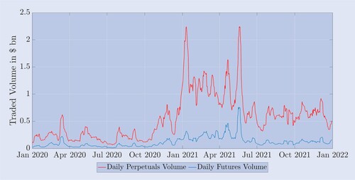
Table 1. Trading volume and open interest of Deribit bitcoin derivatives.

	Options		Futures		Perpetuals
	2020	2021	2020	2021	2020	2021
Average Daily Volume	160	818	63	175	265	851
Average Open Interest	1365	8558	143	1043	113	564
Max Volume	1142	3520	515	2100	1400	4890

Notes: Descriptive statistics of the three main products on the Deribit exchange. The table reports the average trading volume and open interest as well as the highest daily volume in $m. We divide the sample data into two yearly periods for comparison.

3. Bitcoin implied volatility

Figure 2 illustrates the empirical dynamics of the implied volatility curve derived from Deribit options, charting its structure daily over a two and a half year period. The moneyness axis represents the curve of volatility implied from prices of out-of-the-money (OTM) puts to calls, with 0.7 for deep OTM puts to 1.3 for deep OTM calls, with at-the-money (ATM) calls and puts having moneyness one, and we have interpolated the data to represent these moneyness levels at a fixed-maturity of 30 days throughout. More details about the data and its filtering are given in the next section.

Figure 2. Bitcoin implied volatility curves.

Implied volatility curves for bitcoin options with 30-day constant maturity, daily between 1 January 2020 and 30 June 2022, derived from out-of-the-money and at-the-money options. Strike levels range from 30% below to 30% above the current value of the underlying BTC index.

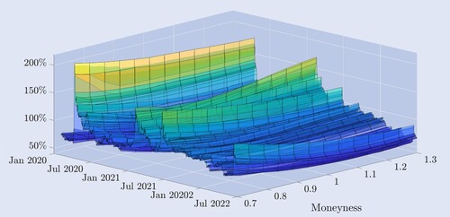
The shape of the curve varies considerably over time. Shortly after the ‘Black Thursday’ event in March 2020, when the bitcoin price fell over 30% in a few hours, the implied volatility curve developed the negative skew shape which is typical of equity index options, where OTM puts have much higher volatility than OTM calls. However, bitcoin options have very much higher implied volatilities than equity index options, in general. During much of the sample period the implied volatility curve resembles a hockey stick, which at particularly tranquil times flattens into a slight symmetric smile. There are also instances of a positive skew, where OTM calls have much higher volatility than OTM puts. The features exhibited are not commonly observed in equity index options markets, where the name ‘skew’ rather than ‘smile’ almost always applies. To support that, figure 3 provides an alternative perspective on the implied volatility smile. It depicts the bitcoin implied volatility for various moneyness levels (upper plot) as well as the deviation from ATM volatility, i.e. the difference between the fixed-moneyness volatility and the ATM volatility (lower plot). Throughout most of the sample, OTM puts with moneyness 0.7 have the highest implied volatility. In traditional (equity) markets, these deep OTM puts are an attractive means of insurance against falling prices. For instance, in the S&P 500 the pronounced and almost linear skew shape of the implied volatility curve means that the option prices that increase most following a fall in the the underlying are those with lowest moneyness. By contrast, figure 3 shows that the bitcoin implied volatility curve was relatively symmetric prior to the crash on 12 March 2020. The lowest volatility of about 50% was for ATM options and both OTM puts and calls had roughly equal but higher volatilities, at around 75% for moneyness 0.7 and 1.3. However, a clear asymmetry in the smile emerged after the crash, with OTM puts drawing a higher premium from risk-averse investors seeking insurance against another significant price drop. The implied volatility of 30-day deep OTM puts suddenly jumped to almost 200%. There was also a pronounced negative skew in bitcoin for the first time, but this shape is still much flatter than the skew one normally observes for equity index options. This asymmetry persisted but gradually diminished as the level of implied volatility dropped and the shape of the implied volatility curve once more began to resemble a smile.

Figure 3. Bitcoin implied volatility and ATM deviation.

Implied volatility curves for bitcoin options with 30-day constant maturity, daily between 1 January 2020 and 30 June 2022 derived from out-of-the-money and at-the-money options for different strike levels ranging from 30% below to 30% above the current value of the underlying BTC index.

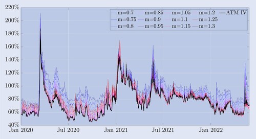
The ATM implied volatility appears to be the lowest point of the smile with a negative skew during most of our sample data but, unlike equity index options, there are periods of high volatility, when the smile has a (strongly) pronounced positive skew. For instance, the slope of the smile increased during bitcoin's rally in June 2021, exhibiting a positive skew for several months. And whereas the equity index price-volatility correlation is almost always large and negative, the correlation between bitcoin and its implied volatility appears to be regime-dependent. From August 2019 to November 2020 the correlation between the bitcoin price and the 30-day ATM implied volatility was around $-0.42$; during the following five months the correlation rose to 0.74 and between July and November 2022 the price-volatility correlation was 0.08.

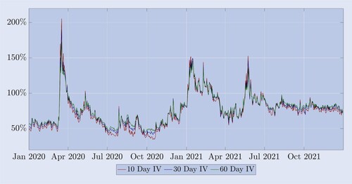
Nevertheless, some features are not unlike those of equity index option implied volatilities: (i) volatilities at different moneyness move along with ATM volatility of the same maturity in a highly correlated fashion, as can be seen in figure 3; and (ii) bitcoin's implied volatility term structure exhibits regular swings between high-volatility periods of backwardation and relatively calm periods of contango. Figure 4 shows that, similar to equity index volatility term structures, bitcoin implied volatilities move along closely with little dispersion during most of the backwardation periods.

Figure 4. Bitcoin implied volatility term structure.

Implied volatility term structure for bitcoin options with 10-, 20 and 30-day constant maturity, daily between 1 January 2020 and 31 December 2021, derived from at-the-money options. It exhibits contango during tranquil periods and the opposite during crash periods (notably March 2020 and June 2021).

We conclude this section by using the characteristics of bitcoin options and futures that we have highlighted above to motivate the rest of this paper. A long bitcoin holder might buy one out-of-the-money put for insurance against a large price fall and consider the spot position suitably hedged. But market makers and other professional traders actively engage in dynamic delta hedging because, as liquidity providers, it is essential for them to hedge the risk of writing options. They could do this using the BS delta, but in view of the popularity among equity option traders of smile-adjusted deltas it is interesting to study the effectiveness of such deltas for bitcoin options. We have reviewed a literature which debates the effectiveness of smile-adjusted deltas for hedging equity index options which reports many circumstances when the BS delta works just as well as any smile-adjusted one. However, no previous study has examined this question for bitcoin options, and it is clear—from the very different behaviour of the bitcoin implied volatility curve that we have just discussed as well as the array of new hedging instruments that are available for bitcoin—that one cannot simply extrapolate what is known about options on equity index options to reach a conclusion about hedging bitcoin options. Therefore, the goal of this study is to introduce and compare the various smile-adjusted deltas that are commonly used by practitioners to analyse their effectiveness for minimising the standard deviation of the hedging error for bitcoin options, based on different choices of hedging instrument. In fact, the study could be extended even further, to the level of the exchange where the option is traded and/or hedged. For instance, is it better to use Binance or Deribit futures or perpetuals to hedge the options listed on the Deribit exchange? But we do not discuss this level of detail of the bitcoin option hedging problem in this study. At least currently, the Deribit options marketplace represents over 90% of trading volume on all bitcoin options at the time of writing, and personal correspondence with the Deribit option market makers indicates that they only use the Deribit futures platform for their delta hedging activities.

4. Hedge ratios

In our experimental design we write a standard European option on a bitcoin index futures worth one bitcoin and delta hedge the position by entering a long position in a certain amount of a futures contract. The T-maturity futures allow traders to enter an agreement to buy or sell a certain amount of bitcoin at a future time T at a bitcoin-USD exchange rate agreed now. The underlying of both futures and options is the Deribit bitcoin index, BTC which is an aggregate non-tradable index. However, we could also hedge a T-maturity option with a position on the perpetual contract, instead of the T-maturity futures contract. We can suppress the running time t in our notation without confusion, and we denote the time t price of an inverse option with strike K and maturity T as $f(K,T\mid F,\sigma )$, where F is either the perpetual price or the T-maturity futures price, at time t, and $\sigma :={\sigma }_t(K,T|F)$ denotes the option's implied volatility also at time t. By incorporating the relationship between volatility and the underlying in our hedging framework, we aim to achieve a more accurate delta than the BS delta, ${\delta }^{BS}$ using a smile-adjusted delta ${\delta }^{adj}$ which is based on the chain rule: (1) $\begin{array}{rl}{\delta }^{adj}(K,T|F,\sigma )& =\frac{\mathrm{\partial }f}{\mathrm{\partial }F}+\frac{\mathrm{\partial }f}{\mathrm{\partial }\sigma }\frac{\mathrm{\partial }\sigma }{\mathrm{\partial }F}\\ & ={\delta }^{BS}(K,T|F,\sigma )+{\nu }_{BS}(K,T|F,\sigma )\\ & \times {\sigma }_F(K,T|F,\sigma ),\end{array}$(1) where ${\delta }^{BS}$ is the standard BS delta, ${\nu }_{BS}$ is the volatility-sensitivity of the BS option price (vega) and ${\sigma }_F=\frac{\mathrm{\partial }\sigma }{\mathrm{\partial }F}$ is the volatility-price sensitivity, i.e. the change in implied volatility for changes in the underlying. While the BS delta and vega have a closed-form formula and are easy to calculate, ${\sigma }_F$ is rather difficult to quantify and several different approaches exist.

The first adjustments to the BS delta that we discuss have their roots in different parameterisations of local volatility depending on the current state of the market, or ‘market regime’. Starting with classic papers by Dupire (1994) and Derman et al. (1996) the concept of local volatility has been developed in a broad-ranging academic literature. Of particular interest here are the ‘sticky models’, advocated by Derman (1999) for hedging equity index options, in the context of applying different parameterisations for the local volatility at the nodes in the binomial tree that models the underlying price evolution. Derman et al. (1996) proposed an approximation to ${\sigma }_F$ as the slope of the implied volatility with respect to the strike:¹³ (2) $\begin{array}{r}{\sigma }_F(K,T|F)\approx k{\sigma }_K(K,T|F),\end{array}$(2) where ${\sigma }_K=\frac{\mathrm{\partial }\sigma }{\mathrm{\partial }K}$ is the derivative of the volatility with respect to the strike level and k should depend on the prevailing market regime. In fact, Derman (1999) introduced three different ‘sticky models’ to represent the behaviour of local volatility in different market regimes. The sticky strike model (SS) describes a trending market situation where he assumes the volatility to be independent of future price movements of the underlying and, as with the BS assumptions, it is constant and the same for every option. The delta in this regime is just equal to the BS delta.¹⁴ The sticky moneyness (SM) (also sometimes called the sticky delta) model considers a range-bounded market. During this regime an option's volatility depends only on its moneyness (or equivalently delta). So the local volatility is again the same at every node in the tree, but each option has a different tree, with a different local volatility, depending on the option's moneyness. As the underlying price moves, so the option's moneyness changes, we must move to a different tree to price the option. Finally, the sticky tree model (ST) captures the local volatility behaviour in a rapidly falling market, i.e. it describes the smile adjustment when there is a strong negative correlation between volatility and the underlying price. This implied tree model gets its name from the local volatility model proposed by Derman and Kani (1994). Again, the local volatility is a deterministic function, but it can be different at each node in the tree, and the same tree is used to price all options. Under these three different types of parameterisation for local volatility, the values for k in (2(2) $\begin{array}{r}{\sigma }_F(K,T|F)\approx k{\sigma }_K(K,T|F),\end{array}$(2) ) would differ according to the market regime, as follows: (3) $\begin{array}{r}k=\{\begin{array}{ll}0& \text{(SS)}\\ 1& \text{(ST)}.\\ -K/F& \text{(SM)}\end{array}\end{array}$(3) Both Crépey (2004) and Alexander et al. (2012) extend the approximation (2(2) $\begin{array}{r}{\sigma }_F(K,T|F)\approx k{\sigma }_K(K,T|F),\end{array}$(2) ) to add state-dependence to k. Also note that a little algebra, combining equations (1) and (2) of Alexander et al. (2012) with equation (3) of Alexander and Nogueira (2007b) shows that the smile-implied, scale-invariant delta of Bates (2005) (which was generalised in Alexander and Nogueira (2007a)) is identical to the sticky moneyness (SM) approximation.

Considering that bitcoin is very volatile, the range of available strikes changes considerably over time. Therefore, to provide the framework for examining options with identical characteristics over a longer time horizon we therefore switch from a strike to a moneyness metric. We define moneyness m as $m=\frac{K}{F}$ and now denote the implied volatility by $\theta (m,T|F)=\sigma (mK,T|F)$. Denoting the partial derivatives of $\theta (m,T|F)$ with respect to F and m as ${\theta }_F(m,T|F)$ and ${\theta }_m(m,T|F)$, respectively, we can rewrite the adjusted delta (7(7) $\begin{array}{r}{\delta }^{mv}(m,T|F)={\delta }^{BS}(m,T|F)+\frac{m}{F}{\nu }_{BS}(K,T|F){\theta }_m(m,T|F).\end{array}$(7) ) as: (4) $\begin{array}{r}{\delta }^{adj}(m,T|F)={\delta }^{BS}(m,T|F)+{\nu }_{BS}(m,T|F){\theta }_F(m,T|F),\end{array}$(4) and also rewrite (2(2) $\begin{array}{r}{\sigma }_F(K,T|F)\approx k{\sigma }_K(K,T|F),\end{array}$(2) ) in the moneyness metric as: (5) $\begin{array}{r}{\theta }_F(m,T|F)\approx \kappa {\theta }_m(m,T|F).\end{array}$(5) We estimate the volatility-price sensitivity ${\theta }_F$ using the local volatility assumptions proposed by Derman (1999) where the type of tree used to model the option price evolution varies according to three possible market regimes: a stable-trending market (SS), a range-bounded market (SM) and a crash-jump regime (ST). This way, translating the sticky deltas of Derman (1999) into the moneyness metric, the values for κ in (5(5) $\begin{array}{r}{\theta }_F(m,T|F)\approx \kappa {\theta }_m(m,T|F).\end{array}$(5) ) should differ according to the market regime as follows: (6) $\begin{array}{r}\kappa =\{\begin{array}{ll}0& \text{(SS)}\\ 1/F& \text{(ST)}.\\ -m/F& \text{(SM)}\end{array}\end{array}$(6) As before, the model-free, smile-implied, scale-invariant delta of Bates (2005) and Alexander and Nogueira (2007a) is identical to the sticky moneyness (SM) delta of Derman and Kani (1994).

Next we consider the minimum variance (MV) delta ${\delta }^{mv}$, i.e. the delta that minimises the instantaneous variance of a delta-hedged portfolio. Here we follow Bakshi et al. (1997) who introduce an approximation which minimises local variance. Lee (2001) shows that this MV hedge ratio has an adjustment of the same size as the (SM) smile-implied delta but with the opposite sign, that is: (7) $\begin{array}{r}{\delta }^{mv}(m,T|F)={\delta }^{BS}(m,T|F)+\frac{m}{F}{\nu }_{BS}(K,T|F){\theta }_m(m,T|F).\end{array}$(7) As explained in detail in Chapter 4 of Alexander (2008), and in other texts on implied volatility, the smile-implied delta produces a counter-intuitive ‘floating smile’ dynamic which also implies that the SM adjustment produces a hedging performance that is significantly worse than the BS delta when the volatility-price correlation is large and negative, i.e. when there is a pronounced negative skew. Since the MV adjustment has the opposite sign to the SM adjustment, the MV delta should out-perform the BS delta for hedging equity index options, and indeed for any option where the implied volatility curve has a marked negative slope.

Our final smile-adjusted delta which we denote ${\delta }^{hw}$ was proposed by Hull and White (2017). It is derived from an empirical estimate of a quadratic relationship between the absolute value of the daily PnL $\mathrm{\Delta }P$ of a BS delta-hedged portfolio with value P, and the BS delta. That is: (8) $\begin{array}{r}y=\frac{{\nu }_{BS}}{\sqrt{\tau }}\frac{\mathrm{\Delta }F}{F}(a+b{\delta }^{BS}+c{\left({\delta }^{BS}\right)}^2)+ϵ.\end{array}$(8) where $\mathrm{\Delta }F$ is the daily PnL of the futures. Having used historical data to obtain the parameter estimates $(\hat{a},\hat{b},\hat{c})$, the Hull and White (HW) delta is then calculated as follows: (9) $\begin{array}{r}{\delta }^{hw}={\delta }^{BS}+\frac{{\nu }_{BS}}{F\sqrt{\tau }}(\hat{a}+\hat{b}{\delta }^{BS}+\hat{c}{\left({\delta }^{BS}\right)}^2)\end{array}$(9) where ${\delta }^{BS}$ and ${\nu }_{BS}$ denote the classic BS delta and vega. The current underlying price is denoted as F, its change is denoted $\mathrm{\Delta }F$ and τ is the option's time to expiry. The authors compute the estimates $(\hat{a},\hat{b},\hat{c})$ using a 36-month rolling window and then analyse the hedging performance of the HW delta, in terms of minimising the standard deviation of the daily hedging error, for S&P 500 and other equity index options over an eleven-year period starting in January 2014. They find improvements from using the HW delta of up to 26%. Other conclusions, which are however entirely based on equity index options, are that it performs better for calls than puts and better for OTM than in-the-money (ITM) options. Moreover, they claim that the HW delta out-performs many other deltas derived from various stochastic and local volatility models, at least when hedging equity index options.

This section has covered a wide range of simple adjustments to the BS delta which which have proven effectiveness in previous studies of hedging options on stock indices and in other traditional asset classes. The question is now whether they can also out-perform a simple BS delta hedge in bitcoin options markets—which are less mature than most traditional options markets, have more pronounced volatility and directional buying pressures, and where market makers rebalance their inventories based on information from these pressures. We summarise the BS-adjusted delta hedge ratios considered in this study in a single formula as follows: (10) $\begin{array}{r}{\delta }^{adj}=\{\begin{array}{ll}{\delta }^{BS}& \text{(SS/BS)}\\ {\delta }^{BS}+{\nu }_{BS}{\theta }_m\frac{1}{F}& \text{(ST)}\\ {\delta }^{BS}-{\nu }_{BS}{\theta }_m\frac{m}{F}& \text{(SM/SI)}.\\ {\delta }^{BS}+{\nu }_{BS}{\theta }_m\frac{m}{F}& \text{(MV)}\\ {\delta }^{BS}+{\nu }_{BS}\frac{1}{F\sqrt{\tau }}(a+b{\delta }^{BS}+c{\left({\delta }^{BS}\right)}^2)& \text{(HW)}\end{array}\end{array}$(10) We conclude with some remarks on the above:

1. The MV adjustment is identical to the ST adjustment when m = 1, i.e. for ATM options, otherwise it is greater in magnitude than the ST adjustment when m>1, i.e. for OTM calls and smaller in magnitude than the ST adjustment when m<1, i.e. for OTM puts;

2. The MV adjustment is always equal and opposite to the SM adjustment, and the SM delta is also the scale-invariant (SI) model-free delta of Alexander and Nogueira (2007a), i.e. the delta of any type of stochastic volatility jump process for the bitcoin option price;

3. The sign of the ST, SM and MV adjustments depends on the slope of the implied volatility curve, ${\theta }_m$. When it has a negative slope the MV and ST deltas are less than—and the SM/SI delta is greater than—the BS/SS delta. When it has a positive slope the MV and ST deltas are greater than—and the SM/SI delta is less than—the BS/SS delta.

5. Data

We have created a unique database by using the exchange API to take hourly snapshots of Deribit option market data over several years. The data contain all level one order book information for all options and futures and the perpetual. In this paper we use data at the eight-hourly and daily frequency only, over a two-year period from 1 January 2020 to 1 January 2022.

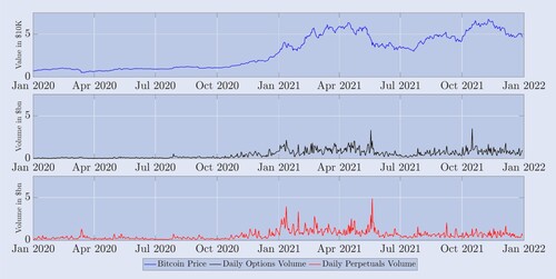
Figure 5 depicts the daily evolution of the settlement price, i.e. the BTC index, at 00:00 UTC and the total traded volumes (as notional amounts, in $bn) of all options and the perpetual on Deribit over the previous 24 hours. Futures contracts are not included here because their trading volumes are very much lower than perpetuals and options, as already seen from figure 1. During 2020, from a level of around $7000, the BTC index rose relatively slowly until its first major bull run starting in November 2020, and the index value reached almost $28,000 by the end of 2020. During 2021 the BTC index more than doubled between January (∼ $28,000) and mid April 2021 (∼$59,000) then fell almost 50% until mid July ($30,000). Its all-time high on 8 November 2021 was around $69,000. The middle plot of figure 5 shows that total 24-hour trading volume over all Deribit options was relatively low during 2020, barely exceeding $500m. However, during 2021 there were pronounced periods of volatile or directional markets where daily options volumes of up to $3bn were commonplace. The number of different options contracts traded also almost doubled, from 4.3 million in January 2021 to 6.2 million by the end of the year. The lower plot depicts the daily trading volume for the perpetual, which was much more active trading during 2021, especially during the first half of the year. Interestingly, the second half of 2021 showed weaker growth in trading on the perpetual than for options. The latter may have been driven by the introduction of many new types of contracts in late 2020 and early 2021, which traders gradually adopted for gamma and vega hedging. By the second half of 2021, this could have diminished the pressure for extremely active dynamic delta hedging. In fact, as seen in figure 1 the volumes traded on futures contracts also fell off—even more so than for the perpetual—during the last six months of 2021. In any case, finding that trading patterns during 2020 were so different from those in 2021 motivates our decision to divide the sample into two one-year periods.

Figure 5. BTC index evolution and daily trading volumes of derivatives.

The upper plot illustrates daily BTC index prices at 00:00 UTC over a two-year sample period starting on 1 January 2020 (top, blue plot); Corresponding 24-hour total trading volume on all Deribit options (middle, black plot); and the daily trading volume on the perpetual (bottom, red plot). Values are given in $10,000 for the BTC index in $bn for trading volumes.

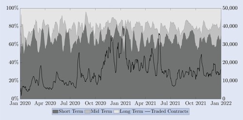
Alexander et al. (2022b) document many differences between the bitcoin and S&P 500 options markets. One of the main differences is the proportion of short-, medium- and long-dated options that are traded. A one-month option on the S&P500 index is considered relatively short term, because the majority of trading occurs between the one-month and the three-month expires. However, a bitcoin option with one-month to expiry falls into the longer-term category. To see this, figure 6 depicts the proportions of daily traded contracts on Deribit based on their time to expiry. On the right-hand scale the solid black line represents the total number of traded contracts traded over all expires. For clarity we present these data using a weekly average on a rolling window. The seasonal pattern in the proportion of short-term (up to two-weeks) options is a result of the issuing schedule policy, whereby options with one week (and/or two weeks) to expiry are issued unless there is a standard monthly or quarterly option expiring with the week (or two weeks). On the left-hand scale we present the proportion of short term (up to two weeks), mid term (between two weeks and a month) and long term (more than a month) maturities. For this, we accumulate all daily traded contracts within each expiry class and present it as percentage over all traded contracts, again using a weekly average on a rolling window for the sake of clarity. Apart from this seasonal pattern, during the entire two-year period only around 15%–20% of trading is on options with expiry dates longer than one month. Even though the number of traded contracts has continually risen over our sample, the proportion of contracts with more than one month to expiry has remained relatively constant, as has the proportion of short term options of up to two weeks. In fact, around 60% of all traded contracts is on these very short-term maturities. Another 20%–25% corresponds to ‘mid-term’ options with maturities between two weeks and one month. Given that the options with maturity of up to one month constitute 80%–85% of all trading volume on Deribit, we decided to focus our hedging study on these options. Options with maturities greater than one month exhibited too many stale prices, even at the hourly frequency, to be useful in our empirical analysis. This motivates us to consider one option for each maturity class documented above. For the sake of easy comparison, we choose 10-, 20- and 30-day constant maturity options for our study, each one being a proxy for the three main expiry classes.

Figure 6. Maturities of traded options.

Proportions (left-hand scale) of total trading volume in short-term options (up to two weeks, dark grey), mid-term options (between two weeks and one month, mid grey) and long-term options (longer than one month, light grey). The black line (right-hand scale) depicts the total number of traded options contracts. All series are a weekly rolling average of daily data.

Next we discuss data filtering. Even just focusing on options with up to one month to expiry, we still needed to filter out some stale prices, i.e. those for options with zero trading volume during the last 24 hours. Liquidity was also a key issue with our data on finite-maturity futures contracts because stale futures prices would induce errors in the option's delta. For this reason, we preferred to use the put-call parity (PCP) relationship to infer the correct futures price, instead of using its market price as we did for the very much more liquid perpetual contract. If needed, we filter out option mid-prices which violate the no-arbitrage conditions proposed by Fengler (2009) and back out the implied volatility from the remaining prices noting that OTM options have very much higher liquidity and trading activity than ITM options of the same strike, so we used the implied volatility of puts for m<1 and calls for $m\ge 1$. Note that the difference between ATM call and put implied volatilities was virtually negligible. This way, we create a raw grid of the market implied volatility surface from which to interpolate filtered prices as described immediately below.

To obtain a continuous historical series for each option price we constructed prices for synthetic, constant-maturity contracts of a given maturity and moneyness. The short-term options are represented by a fixed maturity of 10 days, the mid-term maturity 20 days and for the long-term maturity we consider 30 days to expiration. Given the often trending price of bitcoin, it is not possible to compare the same strike over a long time period so we also selected an appropriate moneyness range for interpolation. We found a maximum range of strikes with sufficient trading volume at around 30% above and below the BTC level. Therefore we interpolated the prices for synthetic options with each fixed maturity, and with a moneyness $m\in \{0.7,0.8,0.9,1,1.1,1.2,1.3\}$.¹⁵ In fact, we used an interpolation over the implied volatility surface, under the no-arbitrage restriction proposed by Fengler (2009), who also proposed a natural cubic spline interpolation to smooth the implied volatility surface. However, the shape of the implied volatility curve for bitcoin moves around much more than it does for other types of options, and we found cubic splines to be too flexible and sensitive to the large intervals between some strikes. Instead we interpolated the implied volatility surface using shape-preserving, piecewise cubic Hermite polynomials and checked the prices afterwards to ensure no violation of the no-arbitrage constraint for convexity with respect to strike. This technique has been applied in numerous other academic studies, e.g. Malz (1997) and Bliss and Panigirtzoglou (2002).

First, we interpolate over the implied volatility smile to obtain a constant moneyness implied volatility using shape-preserving, piecewise cubic Hermite polynomials, again under the no-arbitrage restriction proposed by Fengler (2009). Next, we interpolate over the volatility term structure to obtain the fixed maturity, fixed-moneyness option implied volatility and use this to create a synthetic option price.¹⁶ To avoid any calendar arbitrage possibilities we ensured the total implied variance was always increasing with maturity. To assess hedging performance we also needed to record the price of each synthetic option at the next time increment, without changing the straddling products used to construct the respective option. Only this framework could allow us to record the PnL on a dynamically delta-hedged portfolio. We therefore created synthetic prices for futures and options, using the methodology just described, to obtain option prices with updated moneyness and maturities 9, 19 and 29 days for use in the daily data set. Similarly for the 8-hour data set we constructed futures and options with maturities eight hours less than 10, 20 and 30 days. Overall, we generated around 175,000 synthetic option prices and 88,000 deltas at the daily frequency and over 525,000 synthetic option prices and over 263,000 deltas at the eight-hour frequency.

Next, and in preparation for our hedging study, we examine some empirical characteristics of the bitcoin perpetual contract and compare these with fixed-maturity futures. The settlement price for bitcoin options is not for a tradable contract so we need to use either the futures or the perpetual as the hedging instrument. In this case, the effectiveness of delta hedging an options with a futures contract depends, among other things, on the variability of the basis. To illustrate this variability figure 7 depicts the difference between the market price of the futures (or the perpetual contract) and the BTC index, divided by the BTC index. This percentage basis is given in basis points (bps), on the left-hand scale for the three synthetic fixed-maturity futures, and on the right-hand scale for the basis relative to the perpetual. As a result of the funding rate mechanism, the basis risk of perpetual futures is very low—most of the time it is less than $\pm 10$ bps. But it is also highly variable—for instance, during the COVID crash in March 2020 the perpetual basis reached almost -150 bps. The very tiny basis risk of perpetuals indicates that they could offer better delta hedging instruments than the calendar futures of the same maturity as the option. Unlike the perpetual basis, the bases for the fixed-maturity futures are almost always positive. For 10-day futures the basis can be as high as 100bps, and for longer term futures the basis can even reach 450 bps. Also notice from this figure that the futures curve at 10, 20 and 30 days is normally in contango—in fact, the ordering $F_{30}>F_{20}>F_{10}$ is present for 620 days of the 730-day sample and only in backwardation during March/April 2020 (the COVID crash and its aftermath) and during June/July 2021 (the end of a long bull run in bitcoin).

Figure 7. Difference between spot and perpetual and futures.

The futures price minus the BTC index, divided by the BTC index, in basis points. The right-hand scale measures the % basis for the perpetual futures (black) and the left-hand scale measures the % basis for the futures with constant maturities of 10-, 20- and 30-days (in blue, red and green, respectively). The sample covers two-years starting in January 2020 and daily snapshots are taken at midnight UTC.

Another factor which could determine the success of a dynamic delta-hedging strategy is transaction costs. If bid-ask spreads on the hedging instrument are large then frequent rebalancing of the delta hedge (in our case not only daily, but also every eight hours) could erode the performance of the hedge. Nevertheless, for any given option, the delta cannot range between excessively different values, e.g. a near to ATM call option will always have a delta close to 0.5, whatever model is used—see Vähämaa (2004) for example. So it is only when spreads are large that different rebalancing amounts that might be implied by different deltas would have a significant impact on hedging performance. However, the bid-ask spread for the perpetual is tiny and even that on the calendar futures is small. For the perpetual it rarely exceeds the minimum tick of $0.5, which is between 0.1 bps and 0.25 bps depending on the price level. The calendar futures have a slightly wider bid-ask spread, which also tends to increase with maturity, but these spreads are also very small, throughout our sample. Even for the longest maturity futures the spread rarely exceeds 5 bps, and most the the time it is around 1 bps. Such low spreads will have an insignificant effect on the results of our comparison between different deltas, so we shall ignore them in the following empirical study.

6. Empirical hedging study

Motivated by our discussions in Sections 2, 3 and 5, we regard the inverse option as a plain vanilla FX option, i.e. we convert its bitcoin price to the corresponding USD value using the current value of the option's underlying. We select the fixed maturities for the synthetic, continuous series for futures and options prices to be 10, 20 and 30 days, and the moneyness for the options to be between 0.7 and 1.3. Our data are constructed for rebalancing the hedge either every eight-hours or every day, and the sample spans a two-year period from 1 January 2020 to 1 January 2022 which is divided into two one-year samples for presentation of the results. At each time t we short a European option with moneyness m and maturity T and hedge this with a long position in either the perpetual or the futures contract with the same maturity as the option and record the PnL of this portfolio as the hedging error under the physical measure, in the usual manner—see Hull and White (2017) for example. Intraday market moves can be very considerable and the transactions costs from rebalancing are tiny, as already discussed. Therefore, we set the base frequency for presenting the tables of results to eight hours. We also time the eight-hourly rebalancing with the funding payment on the perpetual, i.e. at 00:00, 08:00 and 16:00 UTC. This is because the rebalancing of a hedge using the perpetual contract could be also be used to make profits from its funding payments.¹⁷

All the deltas in (10(10) $\begin{array}{r}{\delta }^{adj}=\{\begin{array}{ll}{\delta }^{BS}& \text{(SS/BS)}\\ {\delta }^{BS}+{\nu }_{BS}{\theta }_m\frac{1}{F}& \text{(ST)}\\ {\delta }^{BS}-{\nu }_{BS}{\theta }_m\frac{m}{F}& \text{(SM/SI)}.\\ {\delta }^{BS}+{\nu }_{BS}{\theta }_m\frac{m}{F}& \text{(MV)}\\ {\delta }^{BS}+{\nu }_{BS}\frac{1}{F\sqrt{\tau }}(a+b{\delta }^{BS}+c{\left({\delta }^{BS}\right)}^2)& \text{(HW)}\end{array}\end{array}$(10) ) except the HW delta require us to calculate the slope of the implied volatility curve every time we rebalance the hedged portfolio. We examined various numerical techniques to calculate the derivative of the implied volatility curve, finding that fitting a polynomial of degree three was the simplest and most accurate. Given our numerically-derived value for this slope, for each option as defined by its moneyness and maturity, we then applied (10(10) $\begin{array}{r}{\delta }^{adj}=\{\begin{array}{ll}{\delta }^{BS}& \text{(SS/BS)}\\ {\delta }^{BS}+{\nu }_{BS}{\theta }_m\frac{1}{F}& \text{(ST)}\\ {\delta }^{BS}-{\nu }_{BS}{\theta }_m\frac{m}{F}& \text{(SM/SI)}.\\ {\delta }^{BS}+{\nu }_{BS}{\theta }_m\frac{m}{F}& \text{(MV)}\\ {\delta }^{BS}+{\nu }_{BS}\frac{1}{F\sqrt{\tau }}(a+b{\delta }^{BS}+c{\left({\delta }^{BS}\right)}^2)& \text{(HW)}\end{array}\end{array}$(10) ) with the BS delta and vega calculated using the standard BS formulae. For the Hull and White (2017) delta we did not mimic their 36-month in-sample calibration period, which they used their empirical study of equity index options. Bitcoin options do not even have 36 months of useful data available. Besides, bitcoin prices are very much more volatile than S&P 500 index values, which is why we want to consider rebalancing the hedge more than once per day. Taking all these considerations into account, we used a rolling window of 30 observations at the daily frequency and 90 observations at the eight-hourly frequency to calibrate the HW delta parameters. Our results will compare the hedging error using the fixed-maturity futures, and using the perpetuals, with the HW regressions being performed twice, depending on the hedging instrument.

We shall display our results using a standard F-test for the difference in variances, using the BS delta as the benchmark, i.e. the Sticky Strike (SS) delta in (10(10) $\begin{array}{r}{\delta }^{adj}=\{\begin{array}{ll}{\delta }^{BS}& \text{(SS/BS)}\\ {\delta }^{BS}+{\nu }_{BS}{\theta }_m\frac{1}{F}& \text{(ST)}\\ {\delta }^{BS}-{\nu }_{BS}{\theta }_m\frac{m}{F}& \text{(SM/SI)}.\\ {\delta }^{BS}+{\nu }_{BS}{\theta }_m\frac{m}{F}& \text{(MV)}\\ {\delta }^{BS}+{\nu }_{BS}\frac{1}{F\sqrt{\tau }}(a+b{\delta }^{BS}+c{\left({\delta }^{BS}\right)}^2)& \text{(HW)}\end{array}\end{array}$(10) ). First, table 2 presents the results for hedging 10-day, 20-day and 30-day options with moneyness between 0.7 and 1.3, and where each option is hedged with the corresponding fixed-maturity futures and rebalancing is performed every eight hours. The entries in this table and the following tables are the variance ratios, i.e. the variance of the ${\delta }^{adj}$-hedging error relative to the variance of the BS delta-hedging error.

Table 2. F-Test hedging results (8 Hour rebalancing, fixed-maturity futures).

	Moneyness
	0.7	0.8	0.9	1	1.1	1.2	1.3
10 Days
2020
ST		1.164***	1.194***	0.890^++	1.131**	1.298***
SM		0.562^+++	0.714^+++	1.043	1.089*	0.896^++
MV		1.016	1.139**	0.890^++	1.163***	1.463***
HW		1.022	1.098*	1.038	1.296***	1.090*
2021
ST		2.045***	1.125**	0.984	1.054	1.220***
SM		0.986	1.008	1.037	0.841^+++	0.841^+++
MV		1.698***	1.083*	0.984	1.063	1.284***
HW		1.991***	1.651***	1.285***	1.412***	2.782***
20 Days
2020
ST	2.241***	1.679***	1.234***	0.877^++	1.044	1.228***	1.207***
SM	0.693^+++	0.969	0.924^+	1.208***	1.217***	1.184***	1.132***
MV	1.806***	1.476***	1.196***	0.877^++	1.061	1.316***	1.322***
HW	1.073	1.105**	1.299***	1.101*	1.074	1.121**	1.584***
2021
ST	1.972***	1.630***	1.067	1.046	1.037	1.100*	1.179***
SM	1.014	1.029	1.031	1.079	1.039	1.012	0.983
MV	1.673***	1.493***	1.088*	1.046	1.045	1.132**	1.262***
HW	1.037	1.076	1.120**	1.021	1.131**	1.303***	1.104**
30 Days
2020
ST	2.462***	1.657***	1.258***	0.903^++	1.029	1.176***	1.264***
SM	0.713^+++	0.969	0.942	1.181***	1.197***	1.179***	1.144***
MV	1.981***	1.471***	1.223***	0.903^++	1.043	1.247***	1.407***
HW	1.001	1.299***	1.454***	1.172***	1.342***	1.361***	1.369***
2021
ST	1.686***	1.372***	0.966	1.022	1.044	1.102*	1.122**
SM	1.074	1.098*	1.077	1.152***	1.031	0.993	0.998
MV	1.459***	1.287***	1.017	1.022	1.052	1.134**	1.180***
HW	1.024	1.194***	1.241***	1.202***	1.264***	1.135**	1.134***

Notes: Variance ratios and significance levels for one-sided F-tests on the null hypothesis $H_0:{\sigma }_{BS}^2={\sigma }_{delta}^2$ with alternative $H^{+}:{\sigma }_{BS}^2>{\sigma }_{delta}^2$ and $H^{\ast }:{\sigma }_{BS}^2<{\sigma }_{delta}^2$, respectively. Hedges are based on the futures contract with the same maturity as the option, and are rebalanced every eight hours. We compare the variance of the hedging error for different deltas, relative to the variance obtained using the BS delta hedge, and divide the two-year sample into two. We use options with three different maturities and moneyness ranging from 0.7 to 1.3, using OTM put options for moneyness $<1$ and OTM calls for $>1$. The 10%, 5% and 1% significance levels are denoted *, ** and *** respectively for $H^{\ast }$, and similarly for $H^{+}$.

The greater the effectiveness of the hedge the lower the variance of the hedging error and the efficiency gain from using the smile-adjusted delta is one minus this variance ratio. For instance, the SM (smile-implied) delta yields a variance ratio of 0.562 for hedging 10-day puts with moneyness 0.8. This indicates an efficiency gain of $1-0.562=43.8\mathrm{\%}$ compared with the BS delta hedge, which is very significant, so the entry is marked +++. In the tables of variance ratios the superscripts denote the significance of one-sided F-tests on the variance ratios at 10%, 5% and 1%. For instance *** denotes that the ${\delta }^{adj}$-hedging error has a very significantly larger variance than the BS delta-hedging error, at the 1% level. And ++ denotes that the ${\delta }^{adj}$-hedging error has a significantly lower variance than the BS delta-hedging error, at the 5% level.

First consider the results for 2020 in table 2. This part of the sample is characterised by slow but steady rising prices consistent with the Derman (1999) stable-trending regime when we expect the SS delta (BS delta) to provide the most efficient delta hedge, or the range-bounded regime when the SM delta prevails. Overall, the 2020 results in table 2 display a pattern where the success of a particular delta to out-perform the BS hedge depends on the options moneyness, but not its maturity. For instance, for ATM options the ST delta is best.¹⁸ The efficiency gain ranges from 9.7% for 30-day ATM options to 12.3% for 20-day options and 11% for 10-day options. The relative performance of the smile-implied (i.e. SM) delta is in the opposite direction to both the ST and MV deltas, not just for ATM options but for options of all moneyness. It out-performs the BS delta for OTM puts but not for OTM calls (except for 10-day calls with moneyness 1.2). For hedging 20-day deep OTM puts the efficiency gain from using the smile-implied (SM) delta throughout the whole of 2020 was $1-0.693=30.7\mathrm{\%}$, which was very highly significant. And it was almost as high for 30-day deep OTM puts, where the efficiency gain was 28.7%. The efficiency gains from using the smile-implied hedge for other put options were much smaller, between only 3.1% and 7.6%.

Otherwise, for every other option, all the smile-adjusted deltas perform worse than the BS delta. However, this is not really surprising since the bitcoin price was stable-trending during a large part of 2020. The practical HW hedge ratio introduced by Hull and White (2017) and the minimum variance (MV) hedge of Lee (2001) also result in no improvement on the BS delta (except for ATM options for which the MV hedge is identical to the ST one). The HW delta also has a major drawback in that it uses regression to estimate its parameters which makes i.i.d. assumptions not appropriate for bitcoin which is very prone to jumps in returns. The impact of any jump remains within a rolling window for a long time and therefore has a large influence on the HW hedge ratio.

Figures 2 and 5 showed that 2021 was characterised by much higher and more turbulent prices, and an increase in the general level of volatility accompanied by a flatter but still asymmetric smile-shaped implied volatility curve. During the entire year of 2021 the market was characterised by huge swings in the bitcoin price as it ranged between $30,000 and almost $70,000, and as one can see from figure 2 the smile at 30-days became relatively flat towards the end this period. But a flat smile makes the key ingredient the adjusted deltas, i.e. the slope of the smile, almost redundant. So it is not surprising that all smile-adjusted deltas presented no significant improvements on the standard BS hedge ratio during the second year of our sample, for all 20-day and 30-day options. However, the very short-term, 10-day smile exhibited some strange features in 2021, becoming upward sloping during the bull market phases of the bitcoin price. This is why the smile-implied (SM) delta hedge showed some very significant efficiency gains of 15.9% compared with using the BS delta for hedging 10-day OTM call options.

Next, tables 3 and 4 examine the robustness of the results in table 2 in two ways: first by repeating the analysis with rebalancing at the daily frequency (table 3) and then by using the perpetual contract instead of the same-maturity futures as the hedging instrument. The results in table 3 display a similar pattern to those in table 2 except that they are less significant overall—but we are not surprised by this because there are now only 365 instead of 1095 observations per year. They confirm our conclusion from table 2 that no smile-adjusted delta can improve on the BS delta during 2021. In 2020 we also see the same pattern of performance relative to the BS delta, in that the ST delta does out-perform for ATM options but now there is some evidence that the HW deltas also beat BS, for ATM options and OTM puts with moneyness 0.9—but none of these variance ratio statistics are statistically significant.

Table 3. F-Test hedging results (daily rebalancing, fixed-maturity futures).

	Moneyness
	0.7	0.8	0.9	1	1.1	1.2	1.3
10 Days
2020
ST		1.012	1.020	0.953	0.978	1.196**
SM		0.978	1.108	1.083	1.108	0.990
MV		1.001	1.011	0.953	0.990	1.281***
HW		1.091	0.940	0.967	1.150*	1.159*
2021
ST		2.067***	1.218**	0.978	1.046	1.165*
SM		0.987	1.085	1.087	0.992	0.975
MV		1.737***	1.174*	0.978	1.055	1.213**
HW		2.917***	2.324***	2.166***	2.464***	2.591***
20 Days
2020
ST	2.819***	1.029	1.010	0.910^+	0.999	1.206**	1.443***
SM	0.693^+++	1.137	1.102	1.133	1.200**	0.983	0.840^++
MV	2.213***	1.005	1.003	0.910^+	1.008	1.285***	1.630***
HW	1.238**	1.134	0.958	0.992	1.109	1.401***	1.102
2021
ST	2.013***	1.551*	1.049	0.997	1.025	1.090	1.131
SM	1.130	1.210**	1.203**	1.117	1.057	1.013	1.013
MV	1.633***	1.368***	1.031	0.997	1.032	1.120	1.195**
HW	3.271***	2.386***	2.058***	2.135***	2.700***	2.168***	1.796***
30 Days
2020
ST	2.699***	1.061	1.011	0.930	1.019	1.119	1.272***
SM	0.838^+++	1.154*	1.090	1.117	1.142	1.179	0.930
MV	2.115***	1.026	0.959	0.930	1.028	1.172^+	1.401***
HW	1.241**	1.541**	1.129	1.139	1.031	1.129	1.429
2021
ST	1.850***	1.428***	1.022	1.015	1.027	1.093	1.113
SM	1.104	1.198**	1.177*	1.196**	1.059	1.001	1.034
MV	1.527*	1.282***	1.009	1.015	1.034	1.122	1.170
HW	3.554***	3.335***	2.534***	2.072***	2.423***	2.410***	1.852***

Notes: Variance ratios and significance levels for one-sided F-tests on the null hypothesis $H_0:{\sigma }_{BS}^2={\sigma }_{delta}^2$ with alternative $H^{+}:{\sigma }_{BS}^2>{\sigma }_{delta}^2$ and $H^{\ast }:{\sigma }_{BS}^2<{\sigma }_{delta}^2$, respectively. Hedges are based on the corresponding fixed-maturity futures and rebalanced every day. We compare the variance of the hedging error for different deltas, relative to the variance obtained using the BS delta hedge, and divide the two-year sample into two. We use options with three different maturities and moneyness ranging from 0.7 to 1.3, using OTM put options for moneyness $<1$ and OTM calls for $>1$. The 10%, 5% and 1% significance levels are denoted *, ** and *** respectively for $H^{\ast }$, and similarly for $H^{+}$.

Table 4. F-Test hedging results (8 Hour rebalancing, perpetual).

	Moneyness
	0.7	0.8	0.9	1	1.1	1.2	1.3
10 Days
2020
ST		1.134**	1.164***	0.908^+	1.118**	1.363***
SM		0.655^+++	0.709^+++	1.031	1.123**	0.995
MV		0.992	1.112**	0.908^+	1.149**	1.488***
HW		1.080	0.943	0.969	1.329***	1.365***
2021
ST		1.988***	1.089*	0.995	1.040	1.198***
SM		0.996	1.022	1.045	0.860^+++	0.859^+++
MV		1.654***	1.051	0.995	1.048	1.257***
HW		1.791***	1.503***	1.212***	1.358***	2.736***
20 Days
2020
ST	2.275***	1.673***	1.198***	0.932	1.029	1.189***	1.184***
SM	0.742^+++	0.995	0.933	1.150**	1.233***	1.215***	1.144**
MV	1.846***	1.478***	1.166***	0.932	1.045	1.267***	1.290***
HW	1.099	1.367***	1.689***	1.085	1.371***	1.556***	1.384***
2021
ST	1.809***	1.475***	0.957	0.995	1.019	1.077	1.122**
SM	1.104*	1.125**	1.106**	1.057	1.068	1.050	1.038
MV	1.548***	1.370***	0.985	0.995	1.025	1.105**	1.184***
HW	1.280***	1.252***	1.271***	1.245***	1.319***	1.213***	1.400***
30 Days
2020
ST	2.364***	1.597***	1.213***	0.941	0.997	1.138**	1.231***
SM	0.734^+++	0.986***	0.965	1.174***	1.214***	1.195***	1.151**
MV	1.915***	1.426***	1.183***	0.941	1.007	1.198***	1.359***
HW	1.067	1.127***	1.330***	1.191***	1.273***	1.356***	1.428***
2021
ST	1.690***	1.349***	0.958	1.011	1.008	1.066	1.079
SM	1.190***	1.241***	1.206***	1.160***	1.075	1.036	1.057
MV	1.416***	1.221***	0.953	1.011	1.012	1.091*	1.124**
HW	1.220***	1.342***	1.415***	1.259***	1.410***	1.216***	1.390***

Notes: Variance ratios and significance levels for one-sided F-tests on the null hypothesis $H_0:{\sigma }_{BS}^2={\sigma }_{delta}^2$ with alternative $H^{+}:{\sigma }_{BS}^2>{\sigma }_{delta}^2$ and $H^{\ast }:{\sigma }_{BS}^2<{\sigma }_{delta}^2$, respectively. Hedges are based on the perpetual futures and rebalanced every wight hours. We compare the variance of the hedging error for different deltas, relative to the variance obtained using the BS delta hedge, and divide the two-year sample into two. We use options with three different maturities and moneyness ranging from 0.7 to 1.3, using OTM put options for moneyness $<1$ and OTM calls for $>1$. The 10%, 5% and 1% significance levels are denoted *, ** and *** respectively for $H^{\ast }$, and similarly for $H^{+}$.

Table 4 repeats exactly the same analysis as for table 2, with the eight-hour rebalancing frequency, but it uses the perpetual contract as the hedging instrument for all options. We see exactly the same pattern of under- or out-performance of the BS delta as in table 2, with very highly significant efficiency gains for hedging OTM puts using the smile-implied (i.e. SM) delta and the ST/MV delta for ATM options. Apart from the smile-implied (SM) delta hedge which again provides large and significant efficiency gains for hedging 10-day OTM calls, no smile-adjusted delta significantly out-performs the BS delta in 2021. There are also some small ($<5\mathrm{\%}$) efficiency gains from using the ST/MV delta for ATM options and the variance ratios are almost always smaller in table 4 than they are in table 2.

This finding leads us to question weather the perpetual contract provides a better hedging instrument than the futures of the same maturity as the option. To answer this question we examine variance ratios where the numerator is the variance of the perpetual-hedging error, and the denominator is the variance of the futures-hedging error. Again we divide the sample into two one-year periods, and present results by delta (now including the BS delta) and by option and table 5 displays the results. In the table a variance ratio less than (greater than) one indicates that a superior (inferior) hedge is obtained using the perpetual contract. The significance of the F statistics are marked depending on whether the perpetual provides a superior (+) or inferior (*) hedging instrument, compared with the same-maturity futures. It is clear that the results depend little on the moneyness of the option, but more on its maturity and the prevailing market state. For the 10-day options the ratios are mostly less than one for OTM calls. For 20-day and 30-day options some highly significant improvements from hedging with the perpetual are evident, especially during 2021.

Table 5. F-Test futures and perpetual comparison (8 Hour rebalancing).

	Moneyness
	0.7	0.8	0.9	1	1.1	1.2	1.3
10 Days
2020
BSM		1.027	1.031	1.015	0.962	0.924^+
ST		1.001	1.005	1.036	0.952	0.970
SM		1.015	1.023	1.003	0.993	0.996
MV		1.003	1.006	1.036	0.951	0.940
HW		1.086	0.886^++	0.948	0.987	1.158***
2021
BSM		0.982	0.993	1.007	0.992	1.016
ST		0.955	0.961	1.017	0.979	0.998
SM		1.003	1.007	1.015	1.014	1.038
MV		0.957	0.964	1.017	0.978	0.994
HW		0.884^++	0.904^++	0.969	0.954	1.009
20 Days
2020
BSM	0.949	0.987	1.001	0.907^+	0.936	0.966	0.989
ST	0.963	0.984	0.973	0.964	0.923^+	0.935	0.970
SM	1.016	1.014	1.011	0.864^+++	0.948	0.991	1.000
MV	0.970	0.989	0.976	0.964	0.922^+	0.930	0.965
HW	0.883^+++	1.132***	1.225***	0.951***	1.108**	1.254***	0.902^++
2021
BSM	0.896^++	0.870^++	0.864^+++	0.878^++	0.849^+++	0.898^++	0.927
ST	0.822^+++	0.788^+++	0.775^+++	0.835^+++	0.834^+++	0.879^++	0.882^++
SM	0.976	0.952	0.927	0.861^+++	0.873^++	0.931	0.979
MV	0.829^+++	0.799^+++	0.782^+++	0.835^+++	0.833^+++	0.876^++	0.870^++
HW	1.106*	1.012	0.980	1.071	0.991	0.836^+++	1.176***
30 Days
2020
BSM	1.003	1.000	1.022	1.057	1.025	1.022	1.026
ST	0.963	0.964	0.985	1.101	0.993	0.988	0.999
SM	1.033	1.017	1.047	1.050	1.039	1.036	1.033
MV	0.969	0.970	0.989	1.101	0.989	0.982	0.991
HW	1.070	0.867^+++	0.934	1.074	0.972	1.018	1.070
2021
BSM	0.839^+++	0.818^+++	0.850^+++	0.910^++	0.867^+++	0.917^+	0.945
ST	0.841^+++	0.804^+++	0.843^+++	0.900^++	0.837^+++	0.887^++	0.909^+
SM	0.930	0.924^+	0.952	0.917^+	0.905^+++	0.956	0.991
MV	0.815^+++	0.776^+++	0.797^+++	0.900^++	0.835^+++	0.882^++	0.901^++
HW	0.999	0.920^+	0.969	0.953	0.968	0.983	1.158***

Notes: Variance ratios and significance levels for one-sided F-tests on the null hypothesis $H_0:{\sigma }_{fut}^2={\sigma }_{perp}^2$ with alternative $H^{+}:{\sigma }_{fut}^2>{\sigma }_{perp}^2$ and $H^{\ast }:{\sigma }_{fut}^2<{\sigma }_{perp}^2$, respectively. Hedges are based on the corresponding fixed-maturity futures and rebalanced every day. For each delta we compare two variances of the hedging error, the numerator is the variance when the perpetual is the hedging instrument and the denominator is the variance when the hedging instrument is the futures with maturity matching the option. Again we divide the two-year sample into two. We use options with three different maturities and moneyness ranging from 0.7 to 1.3, using OTM put options for moneyness $<1$ and OTM calls for $>1$. The 10%, 5% and 1% significance levels are denoted *, ** and *** respectively for $H^{\ast }$, and similarly for $H^{+}$.

Although the tables of results have provided a big picture about the overall relative efficiency of different smile-adjusted deltas, our two-year sample spans a variety of market regimes. As already observed from figure 5 there are periods when the bitcoin market fluctuated quite quickly between stable-trending, range-bound and crash-jump regimes. So to help understand which delta performed best in which market state, figure 8 depicts time series of the variance ratio, i.e. the variance of the smile-adjusted-delta hedging error divided by the variance of the BS-delta hedging error. This is for rebalancing the hedge every eight hours and now each variance is calculated using only the last 90 observations—the same window as used for the HW delta parameter estimation. We emphasise that a value greater than one indicates that the smile-adjusted delta yields an inferior delta-hedging performance relative to the BS delta and we present the results on a log scale for clarity, so a variance ratio of one translates to zero in these plots. Any line below zero indicates that the delta improves on the BS delta, but a line above zero shows the delta provides a less effective hedge than BS.

Figure 8. Hedging performance on a rolling sample. (a) Results for 10-day Options and (b) Results for 30-day Options.

Variance ratios showing performance of the various perpetuals hedge ratios relative to the BS delta, using 8-hourly rebalancing, where variances of the hedging errors are calculated using the previous 90 observations. We present results for (a) 10-day and (b) 30-day options on a log-scale over the two-year sample. The solid line at 0 acts as a reference value, with ratios above 0 indicating inferior performance relative to BS and ratios below 0 indicating superior performance relative to BS. The top graph in (a) depicts the performance for OTM put options with m = 0.8 and for (b) put options with m = 0.7, the middle graph shows ATM options for both (a) and (b), and the bottom one is OTM call options with (a) moneyness 1.2 and (b) moneyness 1.3.

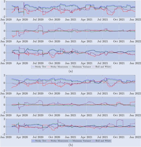
Results for 10-day options are exhibited in the upper set (a) of three plots, and results for 30-day options are exhibited in the lower set (b) of three plots. In each case (a) and (b), the top graph is for OTM put options, and these confirm the results from table 2: both ST (blue) and MV (green) deltas under-perform BS for almost the entire period; as expected from the Derman (1999) classification of regimes, the SM delta out-performs the BS delta during periods when the market is range-bounded but not when it is trending, e.g. during the first big bull run starting in January 2021 and the second bull run later that year; and the performance of the HW delta is mixed. The middle graph of each set presents the variance ratios for hedging ATM options. Here all the smile-adjusted deltas are very similar because the bitcoin smile is often (but not always) quite flat at this point. The bottom graph of each set shows the performance of different deltas for hedging OTM call options. Again the SM delta appears best but only for 10-day options and the improvement over BS is less than it is for OTM put options. For 30-day options no delta provides a sustained improvement over BS, especially during 2021.

7. Conclusion

Previous academic empirical research on model-free smile-implied and regime-dependent smile-adjusted delta hedging has only investigated equity index options. Although the results are mixed, the general consensus of conclusions is that smile-adjusted hedge ratios can only improve on the Black–Scholes delta for out-of-the-money put options, sometimes. But we have shown that bitcoin implied volatility smiles behave very differently from those of equity index options and consequently it is of considerable interest to examine the effectiveness of the smile-adjusted hedge ratios that are often favoured by practitioners.

We motivate the potential use of a variety of adjusted deltas, most of which depend only on the slope of the implied volatility smile curve at the moneyness and maturity of the option that is hedged. Using a unique data set for Deribit options we are able to compare the hedging effectiveness for the most actively traded bitcoin options on the Deribit exchange, i.e. options with strike levels ranging 30% above and below the current BTC index and with expiry up to one month. We analyse the variance of the delta-hedging errors where the hedging instrument is either the futures of the same maturity as the option, or the perpetual contract—this being an innovative product that is unique to crypto currency derivatives markets. With rebalancing of the hedge either every eight hours (to coincide with funding payments on the perpetual) or daily, and using either the same-maturity futures or the perpetual as the hedging instrument, we find some very robust results. Also, rather than a simple tabular comparison of the mean square errors from different hedge ratios as used in Coleman et al. (2001), Vähämaa (2004), Alexander et al. (2012) and many others we have applied a simple variance-ratio test which provides the statistical significance of efficiency gain from using a given delta, relative to the BS delta.

This way we have demonstrated that the smile-implied (sticky-moneyness) delta can provide a significantly better hedge than a standard Black–Scholes delta for out-of-the-money options, with efficiency gains of over 40% in some cases. The minimum-variance delta is also better than the BS delta, but only for at-the-money options, where it coincides with the sticky-tree delta. No other smile-adjusted delta can improve on the Black–Scholes delta consistently, and even the smile-implied and minimum-variance delta hedge performance were poor during much of 2021. The exception is the smile-implied hedge for short-term out-of-the-money calls, at times when the slope of the implied volatility curve became positive. In contrast to equity indices like the S&P500, the bitcoin price does not trends upwards in a stable fashion and then suddenly crash—its upwards price jumps can be as large as its downward price jumps so its smile can be quite symmetric—or even completely upwards sloping. We have also shown that the perpetual contract is a significantly better hedging instrument than the same-maturity futures as the option, irrespective of the option's moneyness. This is particularly evident for options with longer maturity, where the basis between the perpetual and the futures is greatest.

Our study has focused on the robust and model-free framework that is preferred by so many practitioners. We have not looked at hedging using any parametric stochastic and/or local volatility models for the simple fact that the scale-invariance of these processes implies that the deltas are actually model-free, and therefore coincide with the smile-implied delta used in this study. Because we have included the robust, minimum-variance delta of Lee (2001) in our study, so we consider the addition of different stochastic volatility processes for dynamic delta hedging to be a research problem that is not so relevant to the crypto trading industry today.

This paper's focus on dynamic delta hedging with frequent rebalancing may help market makers in bitcoin options gain a competitive edge in a market that only really started to mature in 2021. Yet the market has grown so rapidly that large professional traders such as Jump Trading, Jane Street, XBTO and Cumberland DRW are making bitcoin option markets of volumes regularly reaching $1bn or more per day. And many new expires and option contract sizes are continually being introduced to meet demand—for instance the CME recently launched the micro bitcoin options for retail traders. Nevertheless, bid-ask spreads on bitcoin options are still relatively large, and much higher than they are on bitcoin futures or perpetuals. Hence, the profitability of bitcoin options market making hinges more on accurate dynamic delta hedging than delta-gamma-vega hedging. If spreads on bitcoin options were to reduce in future then it could be interesting to investigate gamma and vega hedging for a bitcoin options book. However, at the time of writing the trading costs of hedging price and volatility risk with options might erode any extra profits made from potentially increasing trading volumes through a reduction in spreads.

Acknowledgments

We are grateful to the anonymous reviewers whose comments led to significant improvement in the paper.

Disclosure statement

The authors report there are no competing interests to declare.

Notes

1 By contrast, the delta derived from a non-scale-invariant model, such as the local volatility model of Dupire (1994), or the sticky-tree model of Derman and Kani (1994), is not theoretically identical to the scale-invariant delta. Neither is a minimum-variance delta, which is the total derivative that includes the vega effect arising from a non-zero price-volatility correlation.

2 See for instance, this recent CAIA article, another one on medium, and several quantitative finance forums such as risklatte and stackexchange.

3 In this strand of the literature, Nastasi et al. (2020) calibrate smile-consistent models for commodity options to capture the smile dynamics and Malz (2000) explains how to take smile adjustments into account when measuring the risk of foreign exchange options.

4 Deribit options have (bi-)daily, (bi-)weekly, (bi-)monthly and quarterly expiry, up to 9 or 12 months. The underlying is the ‘Deribit BTC Index’ (BTC) which is an equally-weighted average of the latest bitcoin price on 11 exchanges, where the highest and lowest price is excluded and the remaining 9 are used to calculate the index. Currently, the exchanges include Binance, Bitfinex, Bitstamp, Bittrex, Coinbase Pro, Gemini, Huobi Global, Itbit, Kraken, LMAX Digital and OKEx and the index is updated every second. There are more option maturities than futures maturities, so in order for Deribit to list option prices in both BTC and USD they use the (possibly synthetic) futures price of the same maturity as the option. This does not imply that the (possibly synthetic) futures contract is the underlying. Indeed, the Deribit options specification documents state that the underlying is the Deribit BTC index. The option strike ranges vary from 50% to 150% of the current BTC price for shorter maturities and up to 800% over the current BTC price for maturities more than six months.

5 See CBOE Historical Options Data for trading volumes on SPX options on the CBOE.

6 See Bitcoin Options Volume and Goldman Sachs Bitcoin Options

7 Second comes the CME (5%), then OKEx (2.5%) and FTX and Bit.com, see The Block Options for more details.

8 To calculate the final payoff, Deribit uses the 30-minute average of of the BTC Index prior to expiry as settlement value, see the official Deribit Options Specification. Note that the Deribit bitcoin options market is not complete. The index itself is not tradable and requires costly replication and frequent rebalancing. The lack of information on the precise calculation of the settlement value results in an incomplete market for traders. However, a detailed discussion of this would exceed the scope of the paper and we refer to Alexander et al. (2022a) for an in-depth discussion.

9 See the 2022 decentralised crypto money market ranking.

10 Inverse futures are bitcoin-denominated futures contracts on the USD-price of a bitcoin or the value of a bitcoin index. Both standard and inverse futures use a USD value as underlying, but their difference lays in their settlement: While standard futures on the CME have a notional of 0.1 or 5 bitcoin and are paid in USD, inverse futures have a notional of $1 or $10 paid in bitcoin. This payment mechanism, on the other hand, results in a different profit and loss (PnL) calculation. For standard futures one subtracts the opening price of the futures from the closing price and multiplies the result by the notional amount, which yields a PnL measured in USD. The settlement procedure for inverse futures (and options) is different, it takes the inverse of the opening price and subtracts from this the inverse of the closing price and then multiplies the result by the notional of the position, which results in a PnL being measured in bitcoin. The ‘opening’ and ‘closing’ price refer to the USD value of a futures contract when entering and exiting a position.

11 See Deribit Perpetual Funding for a description of the Deribit funding rate calculation.

12 See The Block or Coinglass. Note that more than eight exchanges display extraordinary high trading volume. However, we ignore many where volumes are artificially inflated by wash trading.

13 Such an approximation has also been advocated by Coleman et al. (2001) and many other authors since.

14 Derman (1999) calls the SS model ‘a poor man's attempt’ to replicate the BS model with implied volatility trees.

15 Except for the very deep OTM puts (m = 0.7) and calls (m = 1.3) which did not have enough trading volume in the short maturity category. We are able to calculate synthetic prices for only 75% of the time and hence we excluded these options in our final results.

16 Naturally, the PCP values will differ for each strike level. Because trading is generally focused on ATM options it is difficult to find a ITM/OTM strike level for which both calls and puts are actively traded so we use the PCP backed out from ATM options. We interpolate the ATM PCP values of two straddling maturities and use this to obtain the synthetic fixed-maturity option price when necessary.

17 For instance, because we are always long the perpetual in our construction, the funding payment is made by the hedger when the perpetual basis is positive and received by the hedger when the basis is negative. The opposite would be the case for hedging a long options position. Either way, we know from figure 7 that the perpetual basis is variable, sometimes positive and sometimes negative. It would not be difficult to code the hedging algorithm to exit the hedge position entirely just before a funding payment is due, but not if the hedge were due to receive the funding. This type of ‘funding payment play’ is very commonly employed by hedge funds today, in markets that have no regulation to prevent such strategic trading bots from operating. Anyway, we are simply suggesting that a funding payment play could be added to a hedging strategy here—we do not explore the potential profits or losses because this is not a study of high-frequency trading strategies.

18 The ST and MV delta are the same for ATM options, so the results are identical but only in this case.

References

- Alexander, C., Pricing, Hedging and Trading Financial Instruments. Market Risk Analysis III, 2008 (Wiley).
- Alexander, C. and Nogueira, L., Model-free hedge ratios and scale invariant models. J. Bank. Finance, 2007a, 31, 1839–1861.
- Alexander, C. and Nogueira, L., Model-free price hedge ratios for homogeneous claims on tradable assets. Quant. Finance, 2007b, 7(5), 473–479.
- Alexander, C., Rubinov, A., Kalepky, M. and Leontsinis, S., Regime-dependent smile-adjusted delta hedging. J. Futures Mark., 2012, 32(3), 203–229.
- Alexander, C., Chen, D. and Imeraj, A., Inverse and quanto inverse options in a Black–Scholes world. SSRN Working Paper, 2022a.
- Alexander, C., Deng, J., Feng, J. and Wan, H., Net buying pressure and the information in bitcoin option trades. J. Financ. Mark., 2022b. (Article in Press).
- Attie, L., The performance of smile-implied delta hedging. Canadian Derivatives Institute, Technical Note TN 17-01, 2017.
- Bakshi, G., Cao, C. and Chen, Z., Empirical performance of alternative option pricing models. J. Finance, 1997, 52, 2003–2049.
- Bates, D., Hedging the smirk. Finance Res. Lett., 2005, 2(4), 195–200.
- Black, F. and Scholes, M., The pricing of options and corporate liabilities. J. Polit. Econ., 1973, 81(3), 637–654.
- Bliss, R. and Panigirtzoglou, N., Testing the stability of implied probability density functions. J. Bank. Finance, 2002, 26(2-3), 381–422.
- Chen, K. and Huang, Y., Detecting jump risk and jump-diffusion model for bitcoin options pricing and hedging. Math., 2021, 9(20), 2567.
- Chi, Y. and Hao, W., Volatility models for cryptocurrencies and applications in the options market. J. Int. Financ. Mark I., 2021, 75, 101421.
- Coleman, T., Kim, Y., Li, Y. and Verma, A., Dynamic hedging with deterministic local volatility function model. J. Risk, 2001, 4(1), 63–89.
- CryptoCompare, Exchange review. September 2022, 2022.
- Crépey, S., Delta-hedging vega risk?. Quant. Finance, 2004, 4(5), 559–579.
- Derman, E., Regimes of volatility. Risk, 1999, 12(4), 55–59.
- Derman, E. and Kani, I., The volatility smile and its implied tree. Quantitative Strategies Research Notes, 1994.
- Derman, E., Kani, I. and Zou, J., The local volatility surface: Unlocking the information in index option prices. Financ. Anal. J., 1996, 52, 25–36.
- Duffie, D., Pan, J. and Singleton, K., Transform analysis and asset pricing for affine jump diffusions. Econometrica, 2000, 68(6), 1343–1376.
- Dupire, B, Pricing with a smile. Risk Mag., 1994, 7(1), 18–20.
- Fengler, M., Arbitrage-free smoothing of the implied volatility surface. Quant. Finance, 2009, 9(4), 417–428.
- François, P. and Stentoft, L., Smile-implied hedging with volatility risk. J. Futures Mark., 2021, 41(8), 1220–1240.
- Hou, A., Wang, W., Chen, C. and Härdle, W., Pricing cryptocurrency options. J. Financ. Econom., 2020, 18(2), 250–279.
- Hull, J. and White, A., Optimal delta hedging for options. J. Bank. Finance, 2017, 17, 180–190.
- Jalan, A., Matkovskyy, R. and Aziz, S., The bitcoin options market: A first look at pricing and risk. Appl. Econ., 2021, 53(17), 2026–2041.
- Lee, R., Implied and local volatilities under stochastic volatility. Int. J. Theor. Appl. Finance, 2001, 4(1), 45–89.
- Malz, A., Estimating the probability distribution of the future exchange rate from option prices. J. Deriv., 1997, 5(2), 18–36.
- Malz, A., Vega risk and the smile. RiskMetrics Working Paper No. 99–06, 2000.
- Matic, J., Packham, N. and Härdle, W., Hedging cryptocurrency options. SSRN Working Paper, 2021.
- McNeil, A. and Frey, R., Estimation of tail-related risk measures for heteroscedastic financial time series: An extreme value Approach. J. Empir. Finance, 2000, 7(3), 271–300.
- Nastasi, E., Pallavicini, A. and Sartorelli, G., Smile modeling in commodity markets. Int. J. Theor. Appl. Finance, 2020, 23(3), 2050019.
- Sauer, B., Virtual currencies, the money market, and monetary policy. Int. Adv. Econ. Res., 2016, 22, 117–130.
- Siu, T.K. and Elliott, R., Bitcoin option pricing with a SETRA-GARCH model. Eur. J. Finance, 2021, 27(6), 564–595.
- Vähämaa, S., Delta hedging with the smile. Financ. Mark. Portfolio Manage., 2004, 18(3), 241–255.