Principled pasting: attaching tails to risk-neutral probability density functions recovered from option prices

Abstract

The popular ‘curve-fitting’ method of using option prices to construct an underlying asset's risk neutral probability density function (RND) first recovers the interior of the density and then attaches left and right tails. Typically, the tails are constructed so that values of the RND and risk neutral cumulative distribution function (RNCDF) from the interior and the tails match at the attachment points. We propose and demonstrate the feasibility of also requiring that the left and right tails accurately price the options with strikes at the attachment points. Our methodology produces a RND that provides superior pricing performance than earlier curve-fitting methods for both those options used in the construction of the RND and those that were not. We also demonstrate that Put-Call Parity complicates the classification of in and out of sample options.

Keywords:

• Option pricing
• Risk-neutral density
• Put-call parity

JEL Classifications:

• C58
• G13

1. Introduction

For more than thirty years, researchers have employed a wide variety of techniques that use a cross-section of option prices observed at a single point in time to recover an underlying asset's implied RND. One of the more popular of these techniques follows the theoretical insight of Breeden and Litzenberger (1978) that a continuum of $(strikeprice,optionprice)$ pairs can be used to recover the entire RND using the second derivative of the option price with respect to the strike price. However, in practice, only a discrete spacing of such pairs over a limited range is available. Thus, researchers developed ways to interpolate between the limited, discrete spacing. A popular methodology traces out the interior of the RND by fitting a curve to the observed option prices and then taking the second derivative of the call option prices consistent with that curve. In this curve-fitting methodology, left and right tails are then attached to the interior of the RND to complete the entire RND.

Coupled with some assumption(s) concerning attitudes towards risk, a RND can shed light on market views regarding the likelihood of movements in the price of the asset underlying the option contract. However, even absent assumptions about risk, RNDs are incredibly useful constructs for policymakers interested in market participants' views on the value of resources in future states of the world. See Feldman et al. (2015) for elaboration on this point.

Construction of the RND using the curve-fitting technique is a numerically intensive task that requires choices about: the options selected to be used for the construction of the interior of the RND, the space in which to fit a curve to these selected option prices, the functional form of the fitted curve, and the method for attaching the tails. Not surprisingly, variations on the procedure have proliferated, due to both the many decisions required in the construction of the RND as well as the great interest among market practitioners and policymakers in the insights offered by RNDs.

To supplement the usual practice of attaching tails that match interior values for the RND and RNCDF, we propose adding an intuitive and common-sense constraint. Namely, the left (right) tail should accurately price the option, in the set of options used to construct the interior of the RND, with the lowest (highest) strike price. The usual practice makes sure that the left and right tails match the height of the RND and the probability mass given by the RNCDF at the attachment points. Our methodology ensures that the probability mass within the tails is properly located by incorporating the conditional expectation of the asset price finishing below (above) the left (right) attachment point that is embedded in the attachment point option price.

When comparing our methodology to earlier curve-fitting techniques, we assess the quality of the constructed RNDs based on the ability of the relevant integrals of the RND to accurately price options. We pay careful attention to option pricing performance both for those options used in the construction of the interior of the RND (in sample) and those that were not (out of sample). Determining which options are in and out of sample requires some care, as Put-Call Parity blurs the distinction between the two classifications - a consideration that has not featured in earlier work.

Our paper is organized as follows. Section 2 reviews the literature on curve-fitting RND recovery. In section 3 we briefly present the curve-fitting process of recovering the interior of the RND as well as our new approach for attaching the left and right tails. Section 4 discusses the particulars of our application to options on the FTSE 100 Index and outlines two earlier and well-known alternative methods for attaching the tails. Section 5 compares the RNDs from each of the methodologies, focusing on the ability of the different methods to accurately price options. Section 6 offers conclusions.

2. Review of the literature

Longer reviews of the entire RND literature can be found in Jackwerth (2004), Taylor (2005), and Figlewski (2018) with well-crafted, succinct reviews available in Bliss and Panigirtzoglou (2002), Figlewski (2010), Markose and Alentorn (2011), and Lu (2019). In these reviews, the techniques used to recover the RND are often divided into parametric and non-parametric categories and then subdivided into categories such as mixture methods, kernel methods, and curve-fitting methods.¹ Here we only review the literature on curve-fitting methods given that our proposed enhancement directly applies to this technique.

Shimko (1993) is the first application of a RND recovery using the curve-fitting methodology. He uses options on the S&P 500 index, constructs the curve using a quadratic function in $(strikeprice,impliedvolatility)$ space, and adds left and right lognormal tails that match the values of the RND and RNCDF at the attachment points. Working with options on foreign exchange, Malz (1997) advocated fitting the curve in $(calldelta,impliedvolatility)$ space using a quadratic equation where implied volatility is a function of: the at-the-money implied volatility, the distance of delta from 0.5, and the square of the distance of delta from 0.5 with the distances weighted, respectively, by the prices quoted for the risk reversal and strangle option combinations. Campa et al. (1997), also working with options on foreign exchange, create the curve using a natural cubic spline in $(\frac{strikeprice}{forwardrate},impliedvolatility)$ space. Rather than attaching tails to complete the RND, they add pseudo-data points by assuming that the implied volatility is unchanged to the left (right) of the option price with the lowest (highest) strike price.

Bliss and Panigirtzoglou (2002) and Bliss and Panigirtzoglou (2004) combine the methods of Malz (1997) and Campa et al. (1997) in their recovery of RNDs for FTSE 100 Index options and short sterling futures by fitting the curve in $(calldelta,impliedvolatility)$ space using a natural cubic spline and pseudo data points to extend the tails. When constructing the spline, they also use vega weights to reduce the importance of options that are deep out-of-the-money.²

In examinations of options on the S&P 500, Figlewski (2010) and Birru and Figlewski (2012) construct the curve using a fourth degree spline in $(strikeprice,impliedvolatility)$ space with a single knot at the at-the-money strike. Like Shimko (1993), both of these papers attach tails to the interior of the RND by explicitly matching the values from the RND and RNCDF using the three-parameter Generalized Extreme Value distribution rather than the two-parameter lognormal distribution. This allows them to match the RNCDF at a single point and the RND at two points for each tail.

Given its popularity, the curve-fitting method is often included in studies that compare two or more techniques for recovering RNDs. Bliss and Panigirtzoglou (2002) compare the curve-fitting method to a parametric recovery involving a mixture of two lognormals. Bondarenko (2003) introduces the positive convolution approximation method and compares it to the curve-fitting method and six other RND recovery techniques. Bu and Hadri (2007) compare the spline curve-fitting to confluent hypergeometric function methods. Eight different techniques, both parametric and non-parametric, are compared in Lu (2019). Reinke (2020) compares the performance of the methods put forward by Jackwerth (2004) and Figlewski (2010). Bahaludin and Abdullah (2017) focus exclusively on curve-fitting methods, comparing the second and fourth order polynomial approaches to spline approaches. Firm conclusions across all of these studies are difficult to reach given that in some studies a ‘true’ distribution or stochastic process is specified that differs from study to study while in other studies calculated option prices from the recovered RND are compared to the actual option prices used in the recovery. However, the use of the curve-fitting methodology in all of these studies demonstrates its popularity.³

3. RND recovery

Recovery of a single RND requires data on option prices for an underlying asset on a single contract/trading day. These data are usually obtained from an exchange, a market-maker, or a third-party distributor and may be end-of-day settlement prices, time-stamped transactions, or bid/ask listings. Standard practice then selects some subset of the option prices based on data filters meant to screen out erroneous prices or prices that are thought to not accurately reflect market conditions (e.g. options without traded volume or open interest) to create a final dataset.

3.1. Recovering the interior of the RND

Recovery of the interior of the RND typically starts with $\mathrm{N}$ out-of-the-money (OTM) $(strikeprice,optionprice)$ pairs selected by the researcher. A researcher may choose to use all available OTM options to recover the interior of the RND or only a subset of the OTM options. As also discussed in section 4.3, we only use a subset of the available OTM options, based on the option call deltas, to construct the interior of the RND in order to allow for a meaningful out-of-sample comparison across the different methodologies we examine. The top panel of figure 1 provides an illustration of the difference between the in-sample and out-of-sample options for one trading day in our dataset. For typical applications using exchange-traded options such as options on crude oil futures or the FTSE 100, N would usually be in the range of 20 to 70. These N selected OTM options are then transformed via non-parametric techniques into a much larger set of T $(strikeprice,estimatedoptionprice)$ pairs at strikes that are very close together. Commonly, T is a fairly large number on the order of 5000. The interiors of the RNCDF and RND are then calculated by applying numerical derivatives to these T pairs. Examples of this methodology are found in Aït-Sahalia and Duarte (2003), Birru and Figlewski (2012), and Bliss and Panigirtzoglou (2004).

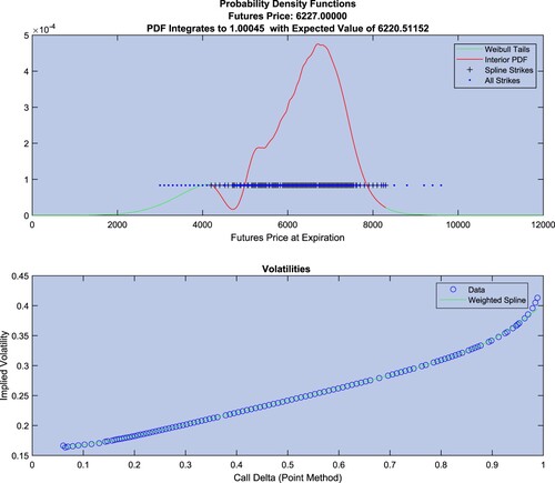
Figure 1. Top Panel: Example risk neutral density constructed using the TailHAP estimation procedure. Bottom Panel: The spline fit in (call delta, implied volatility) space used in the construction of the interior of the risk neutral density shown in red in the top panel.

To fix notation, an $(N,2)$ matrix of observed strike prices and OTM option prices that satisfy monotonicity and convexity constraints is used to ultimately create a $(T,4)$ matrix of tightly-spaced strike prices, theoretical call prices, and the RNCDF and RND evaluated at each tightly-spaced strike price. The process is visualized in equation (1(1) $\begin{array}{rl}& \left[\begin{array}{cc}{K}_1& P_1\\ K_2& P_2\\ ..& ..\\ K_{N-1}& C_{N-1}\\ K_N& C_N\end{array}\right]\\ & ⟹\left[\begin{array}{cccc}{X}_1& \widehat{C_1}& .& .\\ X_2& \widehat{C_2}& RNCD{F}_2& RN{D}_2\\ X_3& \widehat{C_3}& RNCD{F}_3& RN{D}_3\\ ..& ..& ..& ..\\ X_{T-2}& \widehat{C_{T-2}}& RNCD{F}_{T-2}& RN{D}_{T-2}\\ X_{T-1}& \widehat{C_{T-1}}& RNCD{F}_{T-1}& RN{D}_{T-1}\\ X_T& \widehat{C_T}& .& .\end{array}\right]\end{array}$(1) ). (1) $\begin{array}{rl}& \left[\begin{array}{cc}{K}_1& P_1\\ K_2& P_2\\ ..& ..\\ K_{N-1}& C_{N-1}\\ K_N& C_N\end{array}\right]\\ & ⟹\left[\begin{array}{cccc}{X}_1& \widehat{C_1}& .& .\\ X_2& \widehat{C_2}& RNCD{F}_2& RN{D}_2\\ X_3& \widehat{C_3}& RNCD{F}_3& RN{D}_3\\ ..& ..& ..& ..\\ X_{T-2}& \widehat{C_{T-2}}& RNCD{F}_{T-2}& RN{D}_{T-2}\\ X_{T-1}& \widehat{C_{T-1}}& RNCD{F}_{T-1}& RN{D}_{T-1}\\ X_T& \widehat{C_T}& .& .\end{array}\right]\end{array}$(1) where: $K_i$ is an observed strike price, $P_i$ is an observed OTM put price, $C_i$ is an observed OTM call price with $i=1,2,\dots N$, $X_j$ is a constructed, tightly-spaced strike price, $\widehat{C_j}$ is an estimated price for a call option with strike $X_j$, $RNCD{F}_j$ is the RNCDF evaluated at $X_j$, and $PD{F}_j$ is the RND evaluated at $X_j$ with $j=1,2,\dots T$.

Both matrices in equation (1(1) $\begin{array}{rl}& \left[\begin{array}{cc}{K}_1& P_1\\ K_2& P_2\\ ..& ..\\ K_{N-1}& C_{N-1}\\ K_N& C_N\end{array}\right]\\ & ⟹\left[\begin{array}{cccc}{X}_1& \widehat{C_1}& .& .\\ X_2& \widehat{C_2}& RNCD{F}_2& RN{D}_2\\ X_3& \widehat{C_3}& RNCD{F}_3& RN{D}_3\\ ..& ..& ..& ..\\ X_{T-2}& \widehat{C_{T-2}}& RNCD{F}_{T-2}& RN{D}_{T-2}\\ X_{T-1}& \widehat{C_{T-1}}& RNCD{F}_{T-1}& RN{D}_{T-1}\\ X_T& \widehat{C_T}& .& .\end{array}\right]\end{array}$(1) ) are ordered such that $K_{i+1}>K_i$ and $X_{j+1}>X_j$. It will be the case that $X_1=K_1$ and $X_T=K_N$, but otherwise there is no direct correspondence between $X_j$ and $K_i$. The values for $RNCD{F}_1,RND{}_1,RNCD{F}_T,RND{}_T$ are not available because calculating centered, numerical derivatives at these points requires option prices that are outside the observed range $[K_1,K_N]$.

Using the methodology of Bliss and Panigirtzoglou (2004) as an example, the process of moving from observed option prices to the interior RND (that is, moving left to right in equation (1(1) $\begin{array}{rl}& \left[\begin{array}{cc}{K}_1& P_1\\ K_2& P_2\\ ..& ..\\ K_{N-1}& C_{N-1}\\ K_N& C_N\end{array}\right]\\ & ⟹\left[\begin{array}{cccc}{X}_1& \widehat{C_1}& .& .\\ X_2& \widehat{C_2}& RNCD{F}_2& RN{D}_2\\ X_3& \widehat{C_3}& RNCD{F}_3& RN{D}_3\\ ..& ..& ..& ..\\ X_{T-2}& \widehat{C_{T-2}}& RNCD{F}_{T-2}& RN{D}_{T-2}\\ X_{T-1}& \widehat{C_{T-1}}& RNCD{F}_{T-1}& RN{D}_{T-1}\\ X_T& \widehat{C_T}& .& .\end{array}\right]\end{array}$(1) )) involves five steps.

Step 1 - determine the implied volatilities $\left({\sigma }_i\right)$ associated with the $(K_i,P_{i}or{C}_i)$ pairs using a non-linear solver and, for the case of options on futures, the Black (1976) option pricing equation. (2) $\begin{array}{rl}C\left(K_i\right)& =e^{-rt}(F\mathrm{\Phi }\left(d_{1,i}\right)-K_i\mathrm{\Phi }\left(d_{2,i}\right))\mathrm{a}\mathrm{n}\mathrm{d}\\ P\left(K_i\right)& =e^{-rt}(K_i\mathrm{\Phi }\left(-d_{2,i}\right)-F\mathrm{\Phi }\left(-d_{1,i}\right))\\ d_{1,i}& =\frac{\ln \left(\frac{F}{K_i}\right)+\frac{{\sigma }_i^{2}t}{2}}{{\sigma }_i\sqrt{t}}\mathrm{a}\mathrm{n}\mathrm{d}{d}_{2,i}=d_{1,i}-{\sigma }_i\sqrt{t}\end{array}$(2) where F is the futures price for the underlying asset at the current point in time, r is the risk-free rate of interest, t is the time to expiration in years for the option contract, and $\mathrm{\Phi }(\cdot )$ denotes the standard normal cumulative distribution function.

Step 2 - The implied volatility associated with the closest-to-the-money strike price, denoted ${\sigma }_{ATM}$, is used to convert the $K_i$ strike prices into call deltas in what is termed the ‘point conversion’ method by Bu and Hadri (2007) using the equation⁴ (3) ${\mathrm{\Delta }}_i^{C_{point}}=e^{-rt}\mathrm{\Phi }\left(\frac{\ln \left(\frac{F}{K_i}\right)+\frac{{\sigma }_{ATM}^{2}t}{2}}{{\sigma }_{ATM}\sqrt{t}}\right)$(3) Step 3 - A curve is fit to the $({\mathrm{\Delta }}_i^{C_{point}},{\sigma }_i)$ pairs, using a cubic smoothing spline with vega weights (essentially moneyness weights) with vega defined as (4) $Veg{a}_i=e^{-rt}F\varphi \left(d_{1,i}\right)\sqrt{t}$(4) where $\varphi (\cdot )$ is the standard normal probability density function. This curve is then evaluated at T tightly spaced call deltas to recover T predicted implied volatilities denoted $\widehat{{\sigma }_j}$. The tightly-spaced call deltas are generated by first creating T tightly-spaced strike prices $X_1$ through $X_T$ in the interval $[K_1,K_N]$ and then using equation (3(3) ${\mathrm{\Delta }}_i^{C_{point}}=e^{-rt}\mathrm{\Phi }\left(\frac{\ln \left(\frac{F}{K_i}\right)+\frac{{\sigma }_{ATM}^{2}t}{2}}{{\sigma }_{ATM}\sqrt{t}}\right)$(3) ) to convert the strike prices into call deltas.

Step 4 - The tightly spaced $({\mathrm{\Delta }}_j^{C_{point}},\widehat{{\sigma }_j})$ pairs are converted into tightly-spaced $(X_j,\widehat{C_j})$ pairs by solving equation (2(2) $\begin{array}{rl}C\left(K_i\right)& =e^{-rt}(F\mathrm{\Phi }\left(d_{1,i}\right)-K_i\mathrm{\Phi }\left(d_{2,i}\right))\mathrm{a}\mathrm{n}\mathrm{d}\\ P\left(K_i\right)& =e^{-rt}(K_i\mathrm{\Phi }\left(-d_{2,i}\right)-F\mathrm{\Phi }\left(-d_{1,i}\right))\\ d_{1,i}& =\frac{\ln \left(\frac{F}{K_i}\right)+\frac{{\sigma }_i^{2}t}{2}}{{\sigma }_i\sqrt{t}}\mathrm{a}\mathrm{n}\mathrm{d}{d}_{2,i}=d_{1,i}-{\sigma }_i\sqrt{t}\end{array}$(2) ) using $X_j$ and $\widehat{{\sigma }_j}$ in place of the $K_i$ and ${\sigma }_i$. Thus the $(X_j,\widehat{C_j})$ pairs will be consistent with the spline fit in Step 3.

Step 5 - As is detailed in Figlewski (2010), the RNCDF and RND are recovered from the centered numerical first and second derivatives calculated from the $(X_j,\widehat{C_j})$ using (5) $\begin{array}{rl}RNCD{F}_{X_j}& \approx e^{rt}\left[\frac{{\hat{C}}_{j+1}-{\hat{C}}_{j-1}}{X_{j+1}-X_{j-1}}\right]+1\mathrm{a}\mathrm{n}\mathrm{d}\\ RN{D}_{X_j}& \approx e^{rt}\left[\frac{{\hat{C}}_{j+1}-2{\hat{C}}_j+{\hat{C}}_{j-1}}{{(X_{j+1}-X_j)}^2}\right]\end{array}$(5) These five steps suffer from some numerical complications related to the precision of the evaluation of $\mathrm{\Phi }(\cdot )$ in Step 1. As a result some options must be discarded, as discussed in section 4.1. In addition, the tightly-spaced $X_j$ cannot be so tightly spaced that the evaluation of $\mathrm{\Phi }(\cdot )$ in equation (3(3) ${\mathrm{\Delta }}_i^{C_{point}}=e^{-rt}\mathrm{\Phi }\left(\frac{\ln \left(\frac{F}{K_i}\right)+\frac{{\sigma }_{ATM}^{2}t}{2}}{{\sigma }_{ATM}\sqrt{t}}\right)$(3) ) yields ${\mathrm{\Delta }}_j^{C_{point}}={\mathrm{\Delta }}_{j+1}^{C_{point}}$ meaning that some judgment be exercised in how tightly to space the $X_j$.

3.2. Attaching the tails

With the interior of the RND determined as in section 3.1, the left tail (the portion of the RND below $X_2$ ) and the right tail (the portion of the RND above $X_{T-1}$) must be added to complete the RND. A variety of methods are used in the literature, for example adding pseudo data points beyond the range of observed strike prices (Bliss and Panigirtzoglou 2004), pasting on generalized extreme value tails (Figlewski 2010, Birru and Figlewski 2012) or simply rescaling the interior of the RND so that it integrates to 1.0 over the range $[X_2,X_{T-1}]$ (Aït-Sahalia and Duarte 2003).

There are a number of conditions that the attached tails can be forced to satisfy. Perhaps most obviously, the value of the functions used to create the attached tails at $X_2$ and $X_{T-1}$ should match the interior portion of the RND at these two points. Denoting the functions used for the left and right tails as $f_L(\cdot )$ and $f_R(\cdot )$, these two conditions are (6) $f_L\left(X_2\right)=RND{}_2\mathrm{a}\mathrm{n}\mathrm{d}{f}_R\left(X_{T-1}\right)=RND{}_{T-1}$(6) Secondly, the probability mass in the two tail functions should match the probability mass below $X_2$ and above $X_{T-1}$ implied by the RND. That is (7) $\begin{array}{rl}{\int }_0^{X_2}{f}_L\left(F_T\right)\mathrm{d}{F}_T& =RNCD{F}_2\mathrm{a}\mathrm{n}\mathrm{d}\\ {\int }_{X_{T-1}}^{\mathrm{\infty }}{f}_R\left(F_T\right)\mathrm{d}{F}_T& =1-RNCD{F}_{T-1}\end{array}$(7) where $F_T$ denotes the underlying futures price at the contract's expiration. Implicit in equation (7(7) $\begin{array}{rl}{\int }_0^{X_2}{f}_L\left(F_T\right)\mathrm{d}{F}_T& =RNCD{F}_2\mathrm{a}\mathrm{n}\mathrm{d}\\ {\int }_{X_{T-1}}^{\mathrm{\infty }}{f}_R\left(F_T\right)\mathrm{d}{F}_T& =1-RNCD{F}_{T-1}\end{array}$(7) ) are conditions on the support for the two tail functions (8) $\begin{array}{rl}{R}_{X_L}& =\{F_T\in [0,+\mathrm{\infty })|f_L\left(F_T\right)>0\}\mathrm{a}\mathrm{n}\mathrm{d}\\ R_{X_R}& =\{F_T\in [0,+\mathrm{\infty })|f_R\left(F_T\right)>0\}\end{array}$(8) as well as the condition that the probability mass of the entire RND sums to 1.0. (9) $\begin{array}{rl}& {\int }_0^{X_2}{f}_L\left(F_T\right)\mathrm{d}{F}_T+\sum _{j=2}^{T-1}(X_j-X_{j-1})RND{}_j\\ & +{\int }_{X_{T-1}}^{\mathrm{\infty }}{f}_R\left(F_T\right)\mathrm{d}{F}_T=1\end{array}$(9) Our contribution is to also constrain the functions used for the left and right tails to accurately price the observed options with strikes that are extremely close to the attachment points. Accurately pricing these options with strikes $K_1=X_1$ and $K_N=X_T$ provides the best possible means for locating the probability mass contained in the tails of the RND. More formally, and using the fact that an option's price is the discounted, risk-neutral probability-weighted payoff of the option given that it finishes in the money, we have (assuming that the OTM option with strike $K_1=X_1$ is a put, while the OTM option with strike $K_N=X_T$ is a call) (10) $\begin{array}{rl}{P}_1& =e^{-rt}max((X_1-E[F_T\mid F_T<X_1])Pr[F_T<X_1],0)\\ & =e^{-rt}(X_1-\frac{{\int }_0^{X_1}{F}_T{f}_L\left(F_T\right)\mathrm{d}{F}_T}{{\int }_0^{X_1}{f}_L\left(F_T\right)\mathrm{d}{F}_T}){\int }_0^{X_1}{f}_L\left(F_T\right)\mathrm{d}{F}_T\\ & =e^{-rt}{\int }_0^{X_1}(X_1-F_T)f_L\left(F_T\right)\mathrm{d}{F}_T\mathrm{a}\mathrm{n}\mathrm{d}\\ C_N& =e^{-rt}max((E[F_T\mid F_T>X_T]-X_T)Pr[F_T>X_T],0)\\ & =e^{-rt}(\frac{{\int }_{X_T}^{\mathrm{\infty }}{F}_T{f}_R\left(F_T\right)\mathrm{d}{F}_T}{{\int }_{X_T}^{\mathrm{\infty }}{f}_R\left(F_T\right)\mathrm{d}{F}_T}-X_T){\int }_{X_T}^{\mathrm{\infty }}{f}_R\left(F_T\right)\mathrm{d}{F}_T\\ & =e^{-rt}{\int }_{X_T}^{\mathrm{\infty }}(F_T-X_T)f_R\left(F_T\right)\mathrm{d}{F}_T\end{array}$(10) Another possible condition is that the expected value of the entire RND should match the appropriately discounted price of the underlying asset. In the case of options on futures, this condition is written as (11) $\begin{array}{rl}& {\int }_0^{X_2}{F}_T{f}_L\left(F_T\right)\mathrm{d}{F}_T+\sum _{j=2}^{T-1}{X}_j(X_j-X_{j-1})RN{D}_j\\ & +{\int }_{X_{T-1}}^{\mathrm{\infty }}{F}_T{f}_R\left(F_T\right)\mathrm{d}{F}_T=F\end{array}$(11) We do not employ this last condition for two reasons. First, the condition is difficult to enforce when separately creating the left and right tails, and second, the condition can be used as a measure of goodness of fit when evaluating the entire RND after attaching the tails.

We use a 2-parameter Weibull probability density function for the left and right tail functions. Our choice of the Weibull is motivated by several considerations. First, the $[0,\mathrm{\infty })$ support for the Weibull is appropriate for considering assets such as the FTSE 100 with prices that cannot be negative. Second, the Weibull is a very flexible functional form that is relatively tractable. Finally, as emphasized by Savickas (2002), the Weibull easily accomodates the negative skewness typically seen in asset price distributions.⁵ The general form of the 2-parameter Weibull distribution is (12) $\begin{array}{l}PDF:f\left(x\right)={\displaystyle \frac{k}{\lambda }}{\left({\displaystyle \frac{x}{\lambda }}\right)}^{k-1}{e}^{-{\left({\displaystyle \frac{x}{\lambda }}\right)}^k}\\ CDF:F\left(x\right)=1-e^{-{\left({\displaystyle \frac{x}{\lambda }}\right)}^k}\end{array}x\in [0,\mathrm{\infty }),k>0,\lambda >0$(12) In what follows we will also use the gamma function $\mathrm{\Gamma }\left(z\right)$ and its variants, the upper incomplete gamma function $\mathrm{\Gamma }(z,M)$ and the lower incomplete gamma function $\gamma (z,M)$, defined as (13) $\begin{array}{rl}\mathrm{\Gamma }\left(z\right)& ={\int }_0^{\mathrm{\infty }}{\tau }^{z-1}{e}^{-\tau }\mathrm{d}\tau \\ \mathrm{\Gamma }(z,M)& ={\int }_M^{\mathrm{\infty }}\tau y^{z-1}{e}^{-\tau }\mathrm{d}\tau \\ \gamma (z,M)& ={\int }_0^M{\tau }^{z-1}{e}^{-\tau }\mathrm{d}\tau \end{array}$(13)

3.2.1. Left tail

For the left tail we use a ‘scaled’ Weibull PDF: (14) $f_L\left(F_T\right)={\text{β}}_L\frac{k_L}{{\lambda }_L}{\left(\frac{F_T}{{\lambda }_L}\right)}^{k_L-1}{e}^{-{\left(\frac{F_T}{{\lambda }_L}\right)}^{k_L}}\mathrm{w}\mathrm{h}\mathrm{e}\mathrm{r}\mathrm{e}{\text{β}}_L=\frac{RN{D}_2}{f_L\left(X_2\right)}$(14) with ${\text{β}}_L$ defined in order to guarantee the condition in equation (6(6) $f_L\left(X_2\right)=RND{}_2\mathrm{a}\mathrm{n}\mathrm{d}{f}_R\left(X_{T-1}\right)=RND{}_{T-1}$(6) ) that the left tail and the interior RND take on the same value at $X_2$. We then use the left tail conditions in equations (7(7) $\begin{array}{rl}{\int }_0^{X_2}{f}_L\left(F_T\right)\mathrm{d}{F}_T& =RNCD{F}_2\mathrm{a}\mathrm{n}\mathrm{d}\\ {\int }_{X_{T-1}}^{\mathrm{\infty }}{f}_R\left(F_T\right)\mathrm{d}{F}_T& =1-RNCD{F}_{T-1}\end{array}$(7) ) and (10(10) $\begin{array}{rl}{P}_1& =e^{-rt}max((X_1-E[F_T\mid F_T<X_1])Pr[F_T<X_1],0)\\ & =e^{-rt}(X_1-\frac{{\int }_0^{X_1}{F}_T{f}_L\left(F_T\right)\mathrm{d}{F}_T}{{\int }_0^{X_1}{f}_L\left(F_T\right)\mathrm{d}{F}_T}){\int }_0^{X_1}{f}_L\left(F_T\right)\mathrm{d}{F}_T\\ & =e^{-rt}{\int }_0^{X_1}(X_1-F_T)f_L\left(F_T\right)\mathrm{d}{F}_T\mathrm{a}\mathrm{n}\mathrm{d}\\ C_N& =e^{-rt}max((E[F_T\mid F_T>X_T]-X_T)Pr[F_T>X_T],0)\\ & =e^{-rt}(\frac{{\int }_{X_T}^{\mathrm{\infty }}{F}_T{f}_R\left(F_T\right)\mathrm{d}{F}_T}{{\int }_{X_T}^{\mathrm{\infty }}{f}_R\left(F_T\right)\mathrm{d}{F}_T}-X_T){\int }_{X_T}^{\mathrm{\infty }}{f}_R\left(F_T\right)\mathrm{d}{F}_T\\ & =e^{-rt}{\int }_{X_T}^{\mathrm{\infty }}(F_T-X_T)f_R\left(F_T\right)\mathrm{d}{F}_T\end{array}$(10) ) to create a system of two non-linear equations to solve for the left tail parameters $k_L$ and ${\lambda }_L$. The initial forms of the equations are (15) $\begin{array}{rl}& {\int }_0^{X_2}{f}_L\left(F_T\right)\mathrm{d}{F}_T={\int }_0^{X_2}{\text{β}}_L\frac{k_L}{{\lambda }_L}{\left(\frac{F_T}{{\lambda }_L}\right)}^{k_L-1}\\ & \\ & e^{-{\left(\frac{F_T}{{\lambda }_L}\right)}^{k_L}}\mathrm{d}{F}_T={\text{β}}_L(1-e^{-{\left(\frac{X_2}{{\lambda }_L}\right)}^{k_L}})=RNCD{F}_2\mathrm{a}\mathrm{n}\mathrm{d}\\ & {\int }_0^{X_1}(X_1-F_T){\text{β}}_L\frac{k_L}{{\lambda }_L}{\left(\frac{F_T}{{\lambda }_L}\right)}^{k_L-1}{e}^{-{\left(\frac{F_T}{{\lambda }_L}\right)}^{k_L}}\mathrm{d}{F}_T=e^{rt}{P}_1\end{array}$(15) The second condition in equation (15(15) $\begin{array}{rl}& {\int }_0^{X_2}{f}_L\left(F_T\right)\mathrm{d}{F}_T={\int }_0^{X_2}{\text{β}}_L\frac{k_L}{{\lambda }_L}{\left(\frac{F_T}{{\lambda }_L}\right)}^{k_L-1}\\ & \\ & e^{-{\left(\frac{F_T}{{\lambda }_L}\right)}^{k_L}}\mathrm{d}{F}_T={\text{β}}_L(1-e^{-{\left(\frac{X_2}{{\lambda }_L}\right)}^{k_L}})=RNCD{F}_2\mathrm{a}\mathrm{n}\mathrm{d}\\ & {\int }_0^{X_1}(X_1-F_T){\text{β}}_L\frac{k_L}{{\lambda }_L}{\left(\frac{F_T}{{\lambda }_L}\right)}^{k_L-1}{e}^{-{\left(\frac{F_T}{{\lambda }_L}\right)}^{k_L}}\mathrm{d}{F}_T=e^{rt}{P}_1\end{array}$(15) ) can be written as (16) $\begin{array}{rl}& {\text{β}}_L{X}_1{\int }_0^{X_1}\frac{k_L}{{\lambda }_L}{\left(\frac{F_T}{{\lambda }_L}\right)}^{k_L-1}{e}^{-{\left(\frac{F_T}{{\lambda }_L}\right)}^{k_L}}\mathrm{d}{F}_T\\ & -{\text{β}}_L{\int }_0^{X_1}{F}_T\frac{k_L}{{\lambda }_L}{\left(\frac{F_T}{{\lambda }_L}\right)}^{k_L-1}{e}^{-{\left(\frac{F_T}{{\lambda }_L}\right)}^{k_L}}\mathrm{d}{F}_T=e^{rt}{P}_1\mathrm{o}\mathrm{r}\\ & {\text{β}}_L{X}_1(1-e^{-{\left(\frac{X_1}{{\lambda }_L}\right)}^{k_L}})\\ & -{\text{β}}_L{\int }_0^{X_1}{F}_T\frac{k_L}{{\lambda }_L}{\left(\frac{F_T}{{\lambda }_L}\right)}^{k_L-1}{e}^{-{\left(\frac{F_T}{{\lambda }_L}\right)}^{k_L}}\mathrm{d}{F}_T=e^{rt}{P}_1\end{array}$(16) We evaluate the remaining integral in equation (16(16) $\begin{array}{rl}& {\text{β}}_L{X}_1{\int }_0^{X_1}\frac{k_L}{{\lambda }_L}{\left(\frac{F_T}{{\lambda }_L}\right)}^{k_L-1}{e}^{-{\left(\frac{F_T}{{\lambda }_L}\right)}^{k_L}}\mathrm{d}{F}_T\\ & -{\text{β}}_L{\int }_0^{X_1}{F}_T\frac{k_L}{{\lambda }_L}{\left(\frac{F_T}{{\lambda }_L}\right)}^{k_L-1}{e}^{-{\left(\frac{F_T}{{\lambda }_L}\right)}^{k_L}}\mathrm{d}{F}_T=e^{rt}{P}_1\mathrm{o}\mathrm{r}\\ & {\text{β}}_L{X}_1(1-e^{-{\left(\frac{X_1}{{\lambda }_L}\right)}^{k_L}})\\ & -{\text{β}}_L{\int }_0^{X_1}{F}_T\frac{k_L}{{\lambda }_L}{\left(\frac{F_T}{{\lambda }_L}\right)}^{k_L-1}{e}^{-{\left(\frac{F_T}{{\lambda }_L}\right)}^{k_L}}\mathrm{d}{F}_T=e^{rt}{P}_1\end{array}$(16) ) with the following substitutions $\begin{array}{rl}u={\left(\frac{F_T}{{\lambda }_L}\right)}^{k_L}& ⟹F_T={\lambda }_L{u}^{\frac{1}{k_L}}\\ \mathrm{d}u=k_L{\left(\frac{F_T}{{\lambda }_L}\right)}^{k_L-1}\left(\frac{1}{{\lambda }_L}\right)\mathrm{d}{F}_T& ⟹\left(\frac{{\lambda }_L}{k_L}\right)\mathrm{d}u\\ & ={\left(\frac{F_T}{{\lambda }_L}\right)}^{k_L-1}\mathrm{d}{F}_T\end{array}$ transforming the remaining integral to (17) ${\lambda }_L{\int }_0^{{\left(\frac{X_1}{{\lambda }_L}\right)}^{k_L}}{u}^{\frac{1}{k_L}}{e}^{-u}\mathrm{d}u$(17) A second round of substitutions $\begin{array}{rl}\frac{1}{k_L}=z-1& ⟹z=1+\frac{1}{k_L}\\ \tau =u& ⟹\mathrm{d}\tau =\mathrm{d}u\end{array}$ allows equation (17(17) ${\lambda }_L{\int }_0^{{\left(\frac{X_1}{{\lambda }_L}\right)}^{k_L}}{u}^{\frac{1}{k_L}}{e}^{-u}\mathrm{d}u$(17) ) to be written as (18) $\begin{array}{rl}{\lambda }_L{\int }_0^{{\left(\frac{X_1}{{\lambda }_L}\right)}^{k_L}}{\tau }^{z-1}{e}^{-\tau }\mathrm{d}\tau & ={\lambda }_L\gamma (z,{\left(\frac{X_1}{{\lambda }_L}\right)}^{k_L})\\ & ={\lambda }_L\gamma (1+\frac{1}{k_L},{\left(\frac{X_1}{{\lambda }_L}\right)}^{k_L})\end{array}$(18) Substituting the result in equation (18(18) $\begin{array}{rl}{\lambda }_L{\int }_0^{{\left(\frac{X_1}{{\lambda }_L}\right)}^{k_L}}{\tau }^{z-1}{e}^{-\tau }\mathrm{d}\tau & ={\lambda }_L\gamma (z,{\left(\frac{X_1}{{\lambda }_L}\right)}^{k_L})\\ & ={\lambda }_L\gamma (1+\frac{1}{k_L},{\left(\frac{X_1}{{\lambda }_L}\right)}^{k_L})\end{array}$(18) ) into equation (16(16) $\begin{array}{rl}& {\text{β}}_L{X}_1{\int }_0^{X_1}\frac{k_L}{{\lambda }_L}{\left(\frac{F_T}{{\lambda }_L}\right)}^{k_L-1}{e}^{-{\left(\frac{F_T}{{\lambda }_L}\right)}^{k_L}}\mathrm{d}{F}_T\\ & -{\text{β}}_L{\int }_0^{X_1}{F}_T\frac{k_L}{{\lambda }_L}{\left(\frac{F_T}{{\lambda }_L}\right)}^{k_L-1}{e}^{-{\left(\frac{F_T}{{\lambda }_L}\right)}^{k_L}}\mathrm{d}{F}_T=e^{rt}{P}_1\mathrm{o}\mathrm{r}\\ & {\text{β}}_L{X}_1(1-e^{-{\left(\frac{X_1}{{\lambda }_L}\right)}^{k_L}})\\ & -{\text{β}}_L{\int }_0^{X_1}{F}_T\frac{k_L}{{\lambda }_L}{\left(\frac{F_T}{{\lambda }_L}\right)}^{k_L-1}{e}^{-{\left(\frac{F_T}{{\lambda }_L}\right)}^{k_L}}\mathrm{d}{F}_T=e^{rt}{P}_1\end{array}$(16) ) and then into equation (15(15) $\begin{array}{rl}& {\int }_0^{X_2}{f}_L\left(F_T\right)\mathrm{d}{F}_T={\int }_0^{X_2}{\text{β}}_L\frac{k_L}{{\lambda }_L}{\left(\frac{F_T}{{\lambda }_L}\right)}^{k_L-1}\\ & \\ & e^{-{\left(\frac{F_T}{{\lambda }_L}\right)}^{k_L}}\mathrm{d}{F}_T={\text{β}}_L(1-e^{-{\left(\frac{X_2}{{\lambda }_L}\right)}^{k_L}})=RNCD{F}_2\mathrm{a}\mathrm{n}\mathrm{d}\\ & {\int }_0^{X_1}(X_1-F_T){\text{β}}_L\frac{k_L}{{\lambda }_L}{\left(\frac{F_T}{{\lambda }_L}\right)}^{k_L-1}{e}^{-{\left(\frac{F_T}{{\lambda }_L}\right)}^{k_L}}\mathrm{d}{F}_T=e^{rt}{P}_1\end{array}$(15) ) provides the two non-linear equations used to solve for the parameters of the left tail. (19) $\begin{array}{rl}& {\text{β}}_L(1-e^{-{\left(\frac{X_2}{{\lambda }_L}\right)}^{k_L}})=RNCD{F}_2\\ & X_1(1-e^{-{\left(\frac{X_1}{{\lambda }_L}\right)}^{k_L}})-{\lambda }_L\gamma (1+\frac{1}{k_L},{\left(\frac{X_1}{{\lambda }_L}\right)}^{k_L})=\frac{e^{rt}{P}_1}{{\text{β}}_L}\end{array}$(19) These two non-linear equations enforce the conditions found in equations (7(7) $\begin{array}{rl}{\int }_0^{X_2}{f}_L\left(F_T\right)\mathrm{d}{F}_T& =RNCD{F}_2\mathrm{a}\mathrm{n}\mathrm{d}\\ {\int }_{X_{T-1}}^{\mathrm{\infty }}{f}_R\left(F_T\right)\mathrm{d}{F}_T& =1-RNCD{F}_{T-1}\end{array}$(7) ) and (10(10) $\begin{array}{rl}{P}_1& =e^{-rt}max((X_1-E[F_T\mid F_T<X_1])Pr[F_T<X_1],0)\\ & =e^{-rt}(X_1-\frac{{\int }_0^{X_1}{F}_T{f}_L\left(F_T\right)\mathrm{d}{F}_T}{{\int }_0^{X_1}{f}_L\left(F_T\right)\mathrm{d}{F}_T}){\int }_0^{X_1}{f}_L\left(F_T\right)\mathrm{d}{F}_T\\ & =e^{-rt}{\int }_0^{X_1}(X_1-F_T)f_L\left(F_T\right)\mathrm{d}{F}_T\mathrm{a}\mathrm{n}\mathrm{d}\\ C_N& =e^{-rt}max((E[F_T\mid F_T>X_T]-X_T)Pr[F_T>X_T],0)\\ & =e^{-rt}(\frac{{\int }_{X_T}^{\mathrm{\infty }}{F}_T{f}_R\left(F_T\right)\mathrm{d}{F}_T}{{\int }_{X_T}^{\mathrm{\infty }}{f}_R\left(F_T\right)\mathrm{d}{F}_T}-X_T){\int }_{X_T}^{\mathrm{\infty }}{f}_R\left(F_T\right)\mathrm{d}{F}_T\\ & =e^{-rt}{\int }_{X_T}^{\mathrm{\infty }}(F_T-X_T)f_R\left(F_T\right)\mathrm{d}{F}_T\end{array}$(10) ) that the left tail matches the CDF of the interior RND at $X_2$ and correctly prices the option with strike $X_1$ for the particular case of the Weibull distribution.

3.2.2. Right tail

The same scaled Weibull approach is used to create the right tail. (20) $\begin{array}{rl}& f_R\left(F_T\right)={\text{β}}_R\frac{k_R}{{\lambda }_R}{\left(\frac{F_T}{{\lambda }_R}\right)}^{k_R-1}{e}^{-{\left(\frac{F_T}{{\lambda }_R}\right)}^{k_R}}\mathrm{w}\mathrm{h}\mathrm{e}\mathrm{r}\mathrm{e}\\ & {\text{β}}_R=\frac{RN{D}_{T-1}}{f_R\left(X_{T-1}\right)}\end{array}$(20) with ${\text{β}}_R$ defined in order to guarantee the condition in equation (6(6) $f_L\left(X_2\right)=RND{}_2\mathrm{a}\mathrm{n}\mathrm{d}{f}_R\left(X_{T-1}\right)=RND{}_{T-1}$(6) ) that the right tail and the interior RND take on the same value at $X_{T-1}$. We then use the right tail conditions in equations (7(7) $\begin{array}{rl}{\int }_0^{X_2}{f}_L\left(F_T\right)\mathrm{d}{F}_T& =RNCD{F}_2\mathrm{a}\mathrm{n}\mathrm{d}\\ {\int }_{X_{T-1}}^{\mathrm{\infty }}{f}_R\left(F_T\right)\mathrm{d}{F}_T& =1-RNCD{F}_{T-1}\end{array}$(7) ) and (10(10) $\begin{array}{rl}{P}_1& =e^{-rt}max((X_1-E[F_T\mid F_T<X_1])Pr[F_T<X_1],0)\\ & =e^{-rt}(X_1-\frac{{\int }_0^{X_1}{F}_T{f}_L\left(F_T\right)\mathrm{d}{F}_T}{{\int }_0^{X_1}{f}_L\left(F_T\right)\mathrm{d}{F}_T}){\int }_0^{X_1}{f}_L\left(F_T\right)\mathrm{d}{F}_T\\ & =e^{-rt}{\int }_0^{X_1}(X_1-F_T)f_L\left(F_T\right)\mathrm{d}{F}_T\mathrm{a}\mathrm{n}\mathrm{d}\\ C_N& =e^{-rt}max((E[F_T\mid F_T>X_T]-X_T)Pr[F_T>X_T],0)\\ & =e^{-rt}(\frac{{\int }_{X_T}^{\mathrm{\infty }}{F}_T{f}_R\left(F_T\right)\mathrm{d}{F}_T}{{\int }_{X_T}^{\mathrm{\infty }}{f}_R\left(F_T\right)\mathrm{d}{F}_T}-X_T){\int }_{X_T}^{\mathrm{\infty }}{f}_R\left(F_T\right)\mathrm{d}{F}_T\\ & =e^{-rt}{\int }_{X_T}^{\mathrm{\infty }}(F_T-X_T)f_R\left(F_T\right)\mathrm{d}{F}_T\end{array}$(10) ) to create a system of two non-linear equations to solve for the right tail parameters $k_R$ and ${\lambda }_R$. The initial forms of the equations are (21) $\begin{array}{rl}& {\int }_{X_{T-1}}^{\mathrm{\infty }}{f}_R\left(F_T\right)\mathrm{d}{F}_T={\int }_{X_{T-1}}^{\mathrm{\infty }}{\text{β}}_R\frac{k_R}{{\lambda }_R}{\left(\frac{F_T}{{\lambda }_R}\right)}^{k_R-1}{e}^{-{\left(\frac{F_T}{{\lambda }_R}\right)}^{k_R}}\mathrm{d}{F}_T\\ & ={\text{β}}_R(1-{\int }_0^{X_{T-1}}\frac{k_R}{{\lambda }_R}{\left(\frac{F_T}{{\lambda }_R}\right)}^{k_R-1}{e}^{-{\left(\frac{F_T}{{\lambda }_R}\right)}^{k_R}}\mathrm{d}{F}_T)\\ & ={\text{β}}_R\left(e^{-{\left(\frac{X_{T-1}}{{\lambda }_R}\right)}^{k_R}}\right)=1-RNCD{F}_{T-1}\mathrm{a}\mathrm{n}\mathrm{d}\\ & {\int }_{X_T}^{\mathrm{\infty }}(F_T-X_T)f_R\left(F_T\right)\mathrm{d}{F}_T=e^{rt}{C}_N\end{array}$(21) The second condition in equation (21(21) $\begin{array}{rl}& {\int }_{X_{T-1}}^{\mathrm{\infty }}{f}_R\left(F_T\right)\mathrm{d}{F}_T={\int }_{X_{T-1}}^{\mathrm{\infty }}{\text{β}}_R\frac{k_R}{{\lambda }_R}{\left(\frac{F_T}{{\lambda }_R}\right)}^{k_R-1}{e}^{-{\left(\frac{F_T}{{\lambda }_R}\right)}^{k_R}}\mathrm{d}{F}_T\\ & ={\text{β}}_R(1-{\int }_0^{X_{T-1}}\frac{k_R}{{\lambda }_R}{\left(\frac{F_T}{{\lambda }_R}\right)}^{k_R-1}{e}^{-{\left(\frac{F_T}{{\lambda }_R}\right)}^{k_R}}\mathrm{d}{F}_T)\\ & ={\text{β}}_R\left(e^{-{\left(\frac{X_{T-1}}{{\lambda }_R}\right)}^{k_R}}\right)=1-RNCD{F}_{T-1}\mathrm{a}\mathrm{n}\mathrm{d}\\ & {\int }_{X_T}^{\mathrm{\infty }}(F_T-X_T)f_R\left(F_T\right)\mathrm{d}{F}_T=e^{rt}{C}_N\end{array}$(21) ) can be written as (22) $\begin{array}{rl}& {\text{β}}_R{\int }_{X_T}^{\mathrm{\infty }}{F}_T\frac{k_R}{{\lambda }_R}{\left(\frac{F_T}{{\lambda }_R}\right)}^{k_R-1}{e}^{-{\left(\frac{F_T}{{\lambda }_R}\right)}^{k_R}}\mathrm{d}{F}_T\\ & -{\text{β}}_R{X}_T{\int }_{X_T}^{\mathrm{\infty }}\frac{k_R}{{\lambda }_R}{\left(\frac{F_T}{{\lambda }_R}\right)}^{k_R-1}{e}^{-{\left(\frac{F_T}{{\lambda }_R}\right)}^{k_R}}\mathrm{d}{F}_T=e^{rt}{C}_N\mathrm{o}\mathrm{r}\\ & {\text{β}}_R{\int }_{X_T}^{\mathrm{\infty }}{F}_T\frac{k_R}{{\lambda }_R}{\left(\frac{F_T}{{\lambda }_R}\right)}^{k_R-1}{e}^{-{\left(\frac{F_T}{{\lambda }_R}\right)}^{k_R}}\mathrm{d}{F}_T\\ & -{\text{β}}_R{X}_T\left(e^{-{\left(\frac{X_T}{{\lambda }_R}\right)}^{k_R}}\right)=e^{rt}{C}_N\end{array}$(22) We evaluate the remaining integral in equation (22(22) $\begin{array}{rl}& {\text{β}}_R{\int }_{X_T}^{\mathrm{\infty }}{F}_T\frac{k_R}{{\lambda }_R}{\left(\frac{F_T}{{\lambda }_R}\right)}^{k_R-1}{e}^{-{\left(\frac{F_T}{{\lambda }_R}\right)}^{k_R}}\mathrm{d}{F}_T\\ & -{\text{β}}_R{X}_T{\int }_{X_T}^{\mathrm{\infty }}\frac{k_R}{{\lambda }_R}{\left(\frac{F_T}{{\lambda }_R}\right)}^{k_R-1}{e}^{-{\left(\frac{F_T}{{\lambda }_R}\right)}^{k_R}}\mathrm{d}{F}_T=e^{rt}{C}_N\mathrm{o}\mathrm{r}\\ & {\text{β}}_R{\int }_{X_T}^{\mathrm{\infty }}{F}_T\frac{k_R}{{\lambda }_R}{\left(\frac{F_T}{{\lambda }_R}\right)}^{k_R-1}{e}^{-{\left(\frac{F_T}{{\lambda }_R}\right)}^{k_R}}\mathrm{d}{F}_T\\ & -{\text{β}}_R{X}_T\left(e^{-{\left(\frac{X_T}{{\lambda }_R}\right)}^{k_R}}\right)=e^{rt}{C}_N\end{array}$(22) ) with the following substitution $\begin{array}{rl}u={\left(\frac{F_T}{{\lambda }_R}\right)}^{k_R}& ⟹F_T={\lambda }_R{u}^{\frac{1}{k_R}}\\ \mathrm{d}u=k_R{\left(\frac{F_T}{{\lambda }_R}\right)}^{k_R-1}\left(\frac{1}{{\lambda }_R}\right)\mathrm{d}{F}_T& ⟹\left(\frac{{\lambda }_R}{k_R}\right)\mathrm{d}u\\ & ={\left(\frac{F_T}{{\lambda }_R}\right)}^{k_R-1}\mathrm{d}{F}_T\end{array}$ transforming the remaining integral to (23) ${\lambda }_R{\int }_{{\left(\frac{X_N}{{\lambda }_R}\right)}^{k_R}}^{\mathrm{\infty }}{u}^{\frac{1}{k_R}}{e}^{-u}\mathrm{d}u$(23) A second round of substitutions $\begin{array}{rl}\frac{1}{k_R}=z-1& ⟹z=1+\frac{1}{k_R}\\ \tau =u& ⟹\mathrm{d}\tau =\mathrm{d}u\end{array}$ allows equation (23(23) ${\lambda }_R{\int }_{{\left(\frac{X_N}{{\lambda }_R}\right)}^{k_R}}^{\mathrm{\infty }}{u}^{\frac{1}{k_R}}{e}^{-u}\mathrm{d}u$(23) ) to be written as (24) $\begin{array}{rl}{\lambda }_R{\int }_{{\left(\frac{X_T}{{\lambda }_R}\right)}^{k_R}}^{\mathrm{\infty }}{\tau }^{z-1}{e}^{-\tau }\mathrm{d}\tau & ={\lambda }_R\mathrm{\Gamma }(z,{\left(\frac{X_T}{{\lambda }_R}\right)}^{k_R})\\ & ={\lambda }_R\mathrm{\Gamma }(1+\frac{1}{k_R},{\left(\frac{X_T}{{\lambda }_R}\right)}^{k_R})\end{array}$(24) Substituting the result in equation (24(24) $\begin{array}{rl}{\lambda }_R{\int }_{{\left(\frac{X_T}{{\lambda }_R}\right)}^{k_R}}^{\mathrm{\infty }}{\tau }^{z-1}{e}^{-\tau }\mathrm{d}\tau & ={\lambda }_R\mathrm{\Gamma }(z,{\left(\frac{X_T}{{\lambda }_R}\right)}^{k_R})\\ & ={\lambda }_R\mathrm{\Gamma }(1+\frac{1}{k_R},{\left(\frac{X_T}{{\lambda }_R}\right)}^{k_R})\end{array}$(24) ) into equation (22(22) $\begin{array}{rl}& {\text{β}}_R{\int }_{X_T}^{\mathrm{\infty }}{F}_T\frac{k_R}{{\lambda }_R}{\left(\frac{F_T}{{\lambda }_R}\right)}^{k_R-1}{e}^{-{\left(\frac{F_T}{{\lambda }_R}\right)}^{k_R}}\mathrm{d}{F}_T\\ & -{\text{β}}_R{X}_T{\int }_{X_T}^{\mathrm{\infty }}\frac{k_R}{{\lambda }_R}{\left(\frac{F_T}{{\lambda }_R}\right)}^{k_R-1}{e}^{-{\left(\frac{F_T}{{\lambda }_R}\right)}^{k_R}}\mathrm{d}{F}_T=e^{rt}{C}_N\mathrm{o}\mathrm{r}\\ & {\text{β}}_R{\int }_{X_T}^{\mathrm{\infty }}{F}_T\frac{k_R}{{\lambda }_R}{\left(\frac{F_T}{{\lambda }_R}\right)}^{k_R-1}{e}^{-{\left(\frac{F_T}{{\lambda }_R}\right)}^{k_R}}\mathrm{d}{F}_T\\ & -{\text{β}}_R{X}_T\left(e^{-{\left(\frac{X_T}{{\lambda }_R}\right)}^{k_R}}\right)=e^{rt}{C}_N\end{array}$(22) ) and then into equation (21(21) $\begin{array}{rl}& {\int }_{X_{T-1}}^{\mathrm{\infty }}{f}_R\left(F_T\right)\mathrm{d}{F}_T={\int }_{X_{T-1}}^{\mathrm{\infty }}{\text{β}}_R\frac{k_R}{{\lambda }_R}{\left(\frac{F_T}{{\lambda }_R}\right)}^{k_R-1}{e}^{-{\left(\frac{F_T}{{\lambda }_R}\right)}^{k_R}}\mathrm{d}{F}_T\\ & ={\text{β}}_R(1-{\int }_0^{X_{T-1}}\frac{k_R}{{\lambda }_R}{\left(\frac{F_T}{{\lambda }_R}\right)}^{k_R-1}{e}^{-{\left(\frac{F_T}{{\lambda }_R}\right)}^{k_R}}\mathrm{d}{F}_T)\\ & ={\text{β}}_R\left(e^{-{\left(\frac{X_{T-1}}{{\lambda }_R}\right)}^{k_R}}\right)=1-RNCD{F}_{T-1}\mathrm{a}\mathrm{n}\mathrm{d}\\ & {\int }_{X_T}^{\mathrm{\infty }}(F_T-X_T)f_R\left(F_T\right)\mathrm{d}{F}_T=e^{rt}{C}_N\end{array}$(21) ) provides the two non-linear equations used to solve for the parameters of the right tail. (25) $\begin{array}{rl}& {\text{β}}_R\left(e^{-{\left(\frac{X_{T-1}}{{\lambda }_R}\right)}^{k_R}}\right)=1-RNCD{F}_{T-1}\\ & {\lambda }_R\mathrm{\Gamma }(1+\frac{1}{k_R},{\left(\frac{X_T}{{\lambda }_R}\right)}^{k_R})-X_T\left(e^{-{\left(\frac{X_T}{{\lambda }_R}\right)}^{k_R}}\right)=\frac{e^{rt}{C}_N}{{\text{β}}_R}\end{array}$(25) These two non-linear equations enforce the conditions found in equations (7(7) $\begin{array}{rl}{\int }_0^{X_2}{f}_L\left(F_T\right)\mathrm{d}{F}_T& =RNCD{F}_2\mathrm{a}\mathrm{n}\mathrm{d}\\ {\int }_{X_{T-1}}^{\mathrm{\infty }}{f}_R\left(F_T\right)\mathrm{d}{F}_T& =1-RNCD{F}_{T-1}\end{array}$(7) ) and (10(10) $\begin{array}{rl}{P}_1& =e^{-rt}max((X_1-E[F_T\mid F_T<X_1])Pr[F_T<X_1],0)\\ & =e^{-rt}(X_1-\frac{{\int }_0^{X_1}{F}_T{f}_L\left(F_T\right)\mathrm{d}{F}_T}{{\int }_0^{X_1}{f}_L\left(F_T\right)\mathrm{d}{F}_T}){\int }_0^{X_1}{f}_L\left(F_T\right)\mathrm{d}{F}_T\\ & =e^{-rt}{\int }_0^{X_1}(X_1-F_T)f_L\left(F_T\right)\mathrm{d}{F}_T\mathrm{a}\mathrm{n}\mathrm{d}\\ C_N& =e^{-rt}max((E[F_T\mid F_T>X_T]-X_T)Pr[F_T>X_T],0)\\ & =e^{-rt}(\frac{{\int }_{X_T}^{\mathrm{\infty }}{F}_T{f}_R\left(F_T\right)\mathrm{d}{F}_T}{{\int }_{X_T}^{\mathrm{\infty }}{f}_R\left(F_T\right)\mathrm{d}{F}_T}-X_T){\int }_{X_T}^{\mathrm{\infty }}{f}_R\left(F_T\right)\mathrm{d}{F}_T\\ & =e^{-rt}{\int }_{X_T}^{\mathrm{\infty }}(F_T-X_T)f_R\left(F_T\right)\mathrm{d}{F}_T\end{array}$(10) ) that the right tail matches the CDF of the interior RND at $X_{T-1}$ and correctly prices the option with strike $X_T$ for the particular case of the Weibull distribution.

4. Application to FTSE 100 options

To demonstrate the efficacy of our tail pasting procedure, we use daily settlement prices for options on the FTSE 100 Index that are traded on the London International Financial Futures and Options Exchange (LIFFE). These are European-style options that, as explained in Markose and Alentorn (2011), can be treated as options on the FTSE 100 Index futures given that the option contracts and the futures contracts expire on the same day. To provide some assurance that our findings are robust across time, historical settlement prices for the FTSE 100 options were accessed from OptionMetrics' IvyDB product using library subscriptions to Wharton Research Data Services (WRDS) for two time periods: February 6, 2013 through February 2, 2014 using the seven quarterly contracts June 2013 through December 2014 and September 30, 2019 through September 30, 2021 using the twelve quarterly contracts December 2019 through September 2022.⁶ The daily settlement prices on the nineteen underlying FTSE 100 futures contracts were obtained from Bloomberg. We use daily yields on sterling (GBP) LIBOR at the overnight, 1 week, 2 week, and 1–12 month tenors to discount future cash flows, employing a linear interpolation between LIBOR maturities to find the interest rate that matches the maturity of the option contract on each day, using the Intercontinental Exchange as the source for the 2013-2014 LIBOR rates and Bloomberg as the source for the 2019-2021 LIBOR rates.⁷ Across the nineteen contracts (a total of 2912 contract/trading days), we have a total of 495 528 option prices with a recorded settle price and a matching interest rate.

4.1. Data cleaning

Given that these data are end-of-day settlement prices and not actual prices at which trades took place, we must carefully screen the data for anomalies to avoid bizarre behavior in the first and second derivatives used to calculate the internal portion of the RNCDF and RND. We employ a number of filters, discussed below and summarized in table 1, that in total take us from 495 528 options across 2912 contract/trading days to 381 696 options across 2850 contract/trading days.

Table 1. Sequential data filters applied to arrive at the final dataset of 381 696 options used in the estimation and evaluation of risk neutral densities.

Options With Non-Missing Settle Prices in IvyDB	495 528
Less Options Other than First Call and Last Put Priced at 0.5 Index Points	9710
Less Options Priced Above the Upper Bound for Options on Futures	–
Less Options Priced Below the Lower Bound for Options on Futures	2137
Less Violations of Monotonicity	8864
Less Violations of Slope	82
Less Violations of Convexity	60 378
Less Violations of Put-Call Parity	13 856
Less Fewer Than 5 OTM Options	1110
Less Expiration Closer Than 8 Days	8514
Less Inaccurate Implied Volatility	9181
Equals Final Sample Size	381 696

First, the minimum tick on the LIFFE is 0.5 FTSE 100 index points. On any given day, quite a few OTM calls and puts will be assigned a settle price of 0.5. Among the 0.5 priced calls, only the 0.5 priced call with the lowest strike conveys any information, as the calls with higher strikes would have been priced lower were it not for the minimum tick requirement. Among the 0.5 priced puts, only the 0.5 priced put with the highest strike conveys any information, as the puts with lower strikes would have been priced lower were it not for the minimum tick requirement. Thus, we discard all of the calls with a price of 0.5 aside from the 0.5 call with the lowest strike and we discard all of the puts with a price of 0.5 aside from the 0.5 put with the highest strike. As can be seen in table 1, this eliminates 9710 options.

Second, options on futures must satisfy the following no-arbitrage conditions.⁸ (26) $\begin{array}{rl}& (X_i-F)e^{-rt}\le P_i\le X_i{e}^{-rt}\mathrm{a}\mathrm{n}\mathrm{d}\\ & (F-X_i)e^{-rt}\le C_i\le F{e}^{-rt}\end{array}$(26) A total of 2137 of the options violated these conditions—in every case the lower bound.

Third, as detailed in textbooks such as McDonald (2012), option prices must satisfy the following monotonicity, slope, and convexity conditions. (27) $\begin{array}{r}\begin{array}{ccc}Monotonicity& C_i\ge C_{i+1}& P_i\le P_{i+1}\\ Slope& C_i-C_{i+1}<K_{i+1}-K_i& P_{i+1}-P_i<K_{i+1}-K_i\\ Convexity& {\displaystyle \frac{C_i-C_{i+1}}{K_{i+1}-K_i}}<{\displaystyle \frac{C_{i-1}-C_i}{K_i-K_{i-1}}}& {\displaystyle \frac{P_i-P_{i+1}}{K_{i+1}-K_i}}<{\displaystyle \frac{P_{i-1}-P_i}{K_i-K_{i-1}}}\end{array}\end{array}$(27) A total of 69 324 violations of these conditions were found, the vast majority for low-priced options violating the convexity condition even though we retained options where the two sides of the convexity inequalities were equal to each other. All three of these conditions were applied repeatedly across the dataset, as a given violation does not determine which option(s) are generating the violation. This is particularly true for the convexity condition as it involves three options. As a result, and as discussed below, even after these deletions we still use the projection method of Dykstra (1983) to enforce these conditions.

Fourth, we drop all pairs of put and call options that share the same strike and violate put-call parity after allowing for the expenses associated with profiting from the violation. In particular, any put-call pairs that violated put-call parity by more than 5 index points (equivalent to £50) were dropped. In total, 13 856 options were eliminated for put-call parity violations. As discussed in section 5.1 these eliminations will be important when considering whether or not an option should be considered as out of sample.

Fifth, we do not estimate a RND for any contract/day with fewer than 5 OTM options, dropping 1110 options.

Sixth, as a contract approaches maturity, the shrinking horizon means that the RND becomes increasingly degenerate and of less interest for both policymakers and market participants. We drop the 8514 options with 7 or fewer calendar days until expiration.

Finally, as mentioned in section 3.1, the numerical complications involved in evaluating $\mathrm{\Phi }(\cdot )$ means that accurate implied volatilities cannot be calculated for some options. Any numerical software that evaluates $\mathrm{\Phi }(\cdot )$ will have a limit H above which $\mathrm{\Phi }\left(H\right)$ returns 1.0 and a limit L below which $\mathrm{\Phi }\left(L\right)$ returns 0.0.⁹ Accurate implied volatilities can only be recovered for options where (28) $L<\frac{\ln \left(\frac{F}{K_i}\right)+\frac{{\sigma }_i^{2}t}{2}}{{\sigma }_i\sqrt{t}}<H\Rightarrow F{e}^{\frac{{\sigma }_i^{2}t}{2}-{\sigma }_i\sqrt{t}H}<K_i<F{e}^{\frac{{\sigma }_i^{2}t}{2}-{\sigma }_i\sqrt{t}L}$(28) This means that accurate implied volatilities cannot be recovered for options with strike prices that are very deep into the left and right tails of the RND. A total of 9181 options were outside the inequalities in equation (28(28) $L<\frac{\ln \left(\frac{F}{K_i}\right)+\frac{{\sigma }_i^{2}t}{2}}{{\sigma }_i\sqrt{t}}<H\Rightarrow F{e}^{\frac{{\sigma }_i^{2}t}{2}-{\sigma }_i\sqrt{t}H}<K_i<F{e}^{\frac{{\sigma }_i^{2}t}{2}-{\sigma }_i\sqrt{t}L}$(28) ). In every case it is the lower limit that is binding, leading us to drop 9181 options with strikes that are quite low relative to the futures price. For researchers working with small sample sizes, Jäckel (2015) provides a methodology for recovering numerically intractable implied volatilities using a rational approximations approach.

Any attempt to recover the internal portions of the RNCDF and RND via numerical derivatives can yield erratic results if the call options do not satisfy the monotonicity, slope, and convexity conditions in equation (27(27) $\begin{array}{r}\begin{array}{ccc}Monotonicity& C_i\ge C_{i+1}& P_i\le P_{i+1}\\ Slope& C_i-C_{i+1}<K_{i+1}-K_i& P_{i+1}-P_i<K_{i+1}-K_i\\ Convexity& {\displaystyle \frac{C_i-C_{i+1}}{K_{i+1}-K_i}}<{\displaystyle \frac{C_{i-1}-C_i}{K_i-K_{i-1}}}& {\displaystyle \frac{P_i-P_{i+1}}{K_{i+1}-K_i}}<{\displaystyle \frac{P_{i-1}-P_i}{K_i-K_{i-1}}}\end{array}\end{array}$(27) ). We follow the lead of Aït-Sahalia and Duarte (2003), including GAUSS code written by Professor Duarte,¹⁰ and use the projection algorithm of Dykstra (1983) on our 381 696 cleaned option prices to guarantee that the monotonicity, slope, and convexity conditions are strictly satisfied on each of the 2850 contract/trading days. As a result of the earlier data filtering, the adjustments made by the Dykstra algorithm were quite small, with the largest adjustment to any single option amounting to only 4.2 FTSE 100 index points. Across all 2850 contract/days, the average root mean square difference between the day's observed option prices and the Dykstra adjusted option prices was 0.0177 FTSE 100 index points.

4.2. Data description

As can be seen in table 2, the options that remain after the filtering described in section 4.1 are roughly evenly divided between puts and calls and spread fairly evenly across moneyness and time to expiration. The sample categories at the bottom of table 2 denote whether an option was used in the recovery of the RND or not. These sample categories are explained in greater detail in section 5.1. The Moneyness categories are those put forward by Figlewski (2002) based on $\frac{\ln \left(\frac{K}{F}\right)}{\sigma \sqrt{t}}$. The large disparity between puts and calls across moneyness is not surprising. If market participants are aiming to protect against the possibility of large drops in the FTSE 100 Index then we would expect a preponderance of deep OTM options to be puts.

Table 2. Descriptive statistics for the 381 696 options in the dataset across puts and calls by: moneyness, days to expiration, and sample. OTM denotes out of the money, ATM denotes at the money, ITM denotes in the money. In sample options are those used to construct the interior of the risk neutral density. Out of sample options are those options that were not used to construct the interior of the risk neutral density and that do not share a strike with an option used to construct the interior. Quasi out of sample options are the remaining options - those options that share a strike with an in sample option.

	Put	Call
Total	193 479	188 217
Moneyness
Deep OTM	46 061	13 229
OTM	36 756	33 065
ATM	58 777	58 767
ITM	32 978	36 792
Deep ITM	18 907	46 364
Days to Expiration
Less than 60	30 505	28 052
Between 60 and 120	36 924	35 764
Between 120 and 180	36 572	35 938
Between 180 and 240	34 664	34 079
Between 240 and 300	28 940	28 687
Greater Than 300	25 874	25 697
Sample
In Sample	82 655	66 257
Out of Sample	38 563	20 377
Quasi Out of Sample	72 261	101 583

Table 3 provides a slightly different view of the data by providing counts of the number of options across the 2850 trading days in our sample. On average, each contract/trading day has almost 155 options available that are spread fairly evenly across moneyness. About 62 OTM options are used to construct the RND for a typical trading day and the typical trading day has an average of almost 31 truly out of sample options.

Table 3. Descriptive statistics for the number of options available on each trading date in the dataset of 381 696 options across 2850 trading days by: puts and calls, moneyness, and sample. OTM denotes out of the money, ATM denotes at the money, ITM denotes in the money. In sample options are those used to construct the interior of the risk neutral density. Out of sample options are those options that were not used to construct the interior of the risk neutral density and that do not share a strike with an option used to construct the interior. Quasi out of sample options are the remaining options - those options that share a strike with an in sample option.

	Mean	Minimum value	Maximum value
Total	154.48	12	268
Calls	76.12	6	134
Puts	78.58	6	137
Moneyness
Deep OTM Options	27.55	1	73
OTM Options	31.15	1	72
ATM Options	52.23	5	105
ITM Options	31.13	1	74
Deep ITM Options	31.44	1	82
Sample
In Sample Options	62.22	6	124
Out of Sample Options	30.52	1	78
Quasi Out of Sample Options	69.52	6	120

Finally, table 4 presents information on the options and trading days for each of the nineteen contracts in our sample. As our sample includes the main phases of the Covid-19 pandemic, there is a fairly sizable movement in the FTSE 100 index during each contract's life, with a given contract/trading day having between 12 and 268 options from which to select the OTM options for RND construction. As can be seen in the columns labeled In Sample, our RNDs are constructed from as few as 6 to as many as 124 OTM options. Maturities for the contract/trading days range from 8 days to slightly more than one year. Our entire sample comes from a period of very low interest rates with the highest average LIBOR rate for a contract amounting to a bit less than 9 basis points.

Table 4. Descriptive statistics across all 19 contracts for the 381 696 options in the dataset by number of options, number of in sample options, range of the futures price, range of days to expiration, and average LIBOR interest rate.

	Number of Options				In Sample Options		Futures Price		Days to Expiration		LIBOR Rate
		Per Day
	Total	Average	Min	Max	Min	Max	Min	Max	Min	Max	Average
Contract
Jun. 2013	6933	78.78	59	101	19	33	6130.5	6818.0	8	135	0.0051
Sep. 2013	11 909	79.39	59	103	18	35	5979.0	6773.5	8	226	0.0055
Dec. 2013	15 418	77.09	45	96	15	32	5953.0	6754.0	8	317	0.0062
Mar. 2014	14 235	71.53	49	103	20	36	5901.5	6782.0	44	368	0.0067
Jun. 2014	8815	66.28	40	76	18	32	5847.0	6728.5	135	361	0.0072
Sep. 2014	4397	60.23	48	66	22	28	6149.5	6680.5	226	361	0.0078
Dec. 2014	1385	60.22	49	68	25	31	6271.5	6655.5	317	361	0.0085
Dec. 2019	7112	131.70	98	179	27	69	7045.5	7420.0	8	81	0.0073
Mar. 2020	15 169	130.77	97	182	35	60	5297.5	7612.5	8	172	0.0075
Jun. 2020	30 587	172.81	136	261	40	117	4907.0	7529.0	8	263	0.0065
Sep. 2020	41 004	170.14	74	252	28	116	4847.0	7458.0	8	354	0.0057
Dec. 2020	47 585	193.44	81	268	29	124	4841.5	7407.5	8	361	0.0040
Mar. 2021	37 974	154.37	12	210	6	84	4949.5	6829.5	8	361	0.0024
Jun. 2021	37 517	152.51	48	197	18	82	5456.0	7103.0	8	361	0.0012
Sep. 2021	37 376	151.94	32	192	16	87	5412.5	7189.0	8	361	0.0009
Dec. 2021	34 175	174.36	142	192	53	77	6219.0	7156.5	78	361	0.0010
Mar. 2022	18 629	139.02	91	151	37	59	6458.5	7086.0	169	361	0.0013
Jun. 2022	10 405	142.53	108	153	46	67	6619.0	7024.0	260	361	0.0018
Sep. 2022	1071	119.00	115	122	50	56	6671.0	6878.0	351	361	0.0030

4.3. RND construction

As outlined in section 3, a researcher constructing a RND must make a number of choices regarding data and estimation techniques. We discuss the choices made in our new technique (hereafter TailHAP for tails matching the Height, Area, and option Price at the attachment points) and, for comparison, two other procedures in highly cited existing studies from Bliss and Panigirtzoglou (2004, 2002) (hereafter BP) and Birru and Figlewski (2012) and Figlewski (2010) (hereafter FB). Given our interest in the performance of the different procedures for attaching the tails, we make sure that the interiors of the RNDs cover a small enough range so that the left and right tails will have enough mass to significantly influence the pricing of any options as well as to guarantee a useful number of out-of-sample options. To construct the interior of the RND for all of the techniques we only use options with call deltas within the range $[0.05,0.99]$. For example, on trading day 20200619 for the Dec. 2020 contract, the options used for the interior have strikes that range from 4200 to 8300 while the futures settle price for that day was 6227.0. All of the RND constructions are done using MatLab.

4.3.1. TailHAP construction

As described in section 3.1, to begin the construction of the interior of the RND we fit a cubic smoothing spline in $({\mathrm{\Delta }}_i^{C_{point}},{\sigma }_i)$ space with vega weights using MatLab routine csaps with the smoothing parameter set to 0.9. The left and right tails are constructed by using the routine fsolve to find the values for $k_L$ and ${\lambda }_L$ (and thereby ${\text{β}}_L$) that solve the expressions in equation (19(19) $\begin{array}{rl}& {\text{β}}_L(1-e^{-{\left(\frac{X_2}{{\lambda }_L}\right)}^{k_L}})=RNCD{F}_2\\ & X_1(1-e^{-{\left(\frac{X_1}{{\lambda }_L}\right)}^{k_L}})-{\lambda }_L\gamma (1+\frac{1}{k_L},{\left(\frac{X_1}{{\lambda }_L}\right)}^{k_L})=\frac{e^{rt}{P}_1}{{\text{β}}_L}\end{array}$(19) ) and the values for $k_R$ and ${\lambda }_R$ (and thereby ${\text{β}}_R$) that solve the expressions in equation (25(25) $\begin{array}{rl}& {\text{β}}_R\left(e^{-{\left(\frac{X_{T-1}}{{\lambda }_R}\right)}^{k_R}}\right)=1-RNCD{F}_{T-1}\\ & {\lambda }_R\mathrm{\Gamma }(1+\frac{1}{k_R},{\left(\frac{X_T}{{\lambda }_R}\right)}^{k_R})-X_T\left(e^{-{\left(\frac{X_T}{{\lambda }_R}\right)}^{k_R}}\right)=\frac{e^{rt}{C}_N}{{\text{β}}_R}\end{array}$(25) ). Solving these highly non-linear equations involving $\mathrm{\Gamma }(z,M)$ and $\gamma (z,M)$ requires good starting values $k_{L0}$, ${\lambda }_{L0}$, $k_{R0}$, and ${\lambda }_{R0}$ that are set as described in the Appendix. Figure 1 provides an example of one trading day's results for the TailHAP procedure, using the results for 20200619 for the Dec. 2020 contract mentioned above. The upper panel shows the entire RND along with the option prices available for that trading day. The + signs denote the options used to construct the interior of the RND. The bottom panel shows the spline in $({\mathrm{\Delta }}_i^{C_{point}},{\sigma }_i)$ space used to create the interior of the PDF. The circles denote the same + options from the top panel.

We also consider a variant of the TailHAP procedure that avoids the $\mathrm{\Gamma }(z,M)$ and $\gamma (z,M)$ functions, denoted TailHAPAlt, where the left and right tails use lognormal densities rather than Weibull densities. The procedure is identical in that the parameters for ‘scaled’ lognormal tails are chosen to match the values of RND and RNCDF at the attachment points as well as the prices of the OTM options with the lowest and highest strike prices. Using some of the results for the lognormal distribution from the Appendix, for the left tail we use fsolve to find the values for ${\mu }_L$ and $\sigma {}_L$ such that (29) $\begin{array}{rl}& {\text{β}}_L\mathrm{\Phi }\left(\frac{\ln \left(X_2\right)-{\mu }_L}{{\sigma }_L\sqrt{t}}\right)=RNCD{F}_2\\ & X_1\mathrm{\Phi }\left(\frac{\ln \left(X_1\right)-{\mu }_L}{{\sigma }_L\sqrt{t}}\right)-e^{{\mu }_L+\frac{{\sigma }_L^{2}t}{2}}\mathrm{\Phi }\left(\frac{\ln \left(X_1\right)-{\mu }_L-{\sigma }_L^{2}t}{{\sigma }_L\sqrt{t}}\right)\\ & =\frac{e^{rt}{P}_1}{{\text{β}}_L}\end{array}$(29) For the right tail we use fsolve to find the values for ${\mu }_R$ and $\sigma {}_R$ such that (30) $\begin{array}{rl}& {\text{β}}_R(1-\mathrm{\Phi }\left(\frac{\ln \left(X_{T-1}\right)-{\mu }_R}{{\sigma }_R\sqrt{t}}\right))=1-RNCD{F}_{T-1}\\ & e^{{\mu }_R+\frac{{\sigma }_R^{2}t}{2}}\mathrm{\Phi }\left(\frac{{\mu }_R+{\sigma }_R^{2}t-\ln \left(X_T\right)}{{\sigma }_R\sqrt{t}}\right)-X_T\mathrm{\Phi }\left(\frac{{\mu }_R-\ln \left(X_T\right)}{{\sigma }_R\sqrt{t}}\right)\\ & =\frac{e^{rt}{C}_N}{{\text{β}}_R}\end{array}$(30) Starting values for equations equations (29(29) $\begin{array}{rl}& {\text{β}}_L\mathrm{\Phi }\left(\frac{\ln \left(X_2\right)-{\mu }_L}{{\sigma }_L\sqrt{t}}\right)=RNCD{F}_2\\ & X_1\mathrm{\Phi }\left(\frac{\ln \left(X_1\right)-{\mu }_L}{{\sigma }_L\sqrt{t}}\right)-e^{{\mu }_L+\frac{{\sigma }_L^{2}t}{2}}\mathrm{\Phi }\left(\frac{\ln \left(X_1\right)-{\mu }_L-{\sigma }_L^{2}t}{{\sigma }_L\sqrt{t}}\right)\\ & =\frac{e^{rt}{P}_1}{{\text{β}}_L}\end{array}$(29) ) and (30(30) $\begin{array}{rl}& {\text{β}}_R(1-\mathrm{\Phi }\left(\frac{\ln \left(X_{T-1}\right)-{\mu }_R}{{\sigma }_R\sqrt{t}}\right))=1-RNCD{F}_{T-1}\\ & e^{{\mu }_R+\frac{{\sigma }_R^{2}t}{2}}\mathrm{\Phi }\left(\frac{{\mu }_R+{\sigma }_R^{2}t-\ln \left(X_T\right)}{{\sigma }_R\sqrt{t}}\right)-X_T\mathrm{\Phi }\left(\frac{{\mu }_R-\ln \left(X_T\right)}{{\sigma }_R\sqrt{t}}\right)\\ & =\frac{e^{rt}{C}_N}{{\text{β}}_R}\end{array}$(30) ) require much less thought, given that $\mathrm{\Phi }(\cdot )$ is more tractable than $\gamma (z,M)$ and $\mathrm{\Gamma }(z,M)$. We use ${\mu }_{L0}={\mu }_{R0}=\ln \left(F\right)-\frac{{\sigma }_{ATM}^{2}t}{2}$ and ${\sigma }_{L0}={\sigma }_{R0}={\sigma }_{ATM}$.

4.3.2. BP construction

To allow for an apples to apples comparison of the RNDs from the different procedures, when constructing the BP RND we deviate slightly from the exact procedure followed by Bliss and Panigirtzoglou (2004, 2002). In their work, Bliss and Panigirtzoglou add two pseudo data points in $(K,\sigma )$ space: one below the lowest strike at $(K_1-150,{\sigma }_1)$ and one above the highest strike at $(K_N+150,{\sigma }_N)$. That is, they extend the volatility smile in either direction by 150 index points by forcing the smile to become horizontal at either end. They then construct the RND as in section 2. They state that ‘Extrapolating the implied volatility function manner has the effect of smoothly pasting log-normal tails onto the density function beyond the range of strikes.’ ¹¹ We accomplish this same pasting by directly formulating lognormal tails that allow us to evaluate the entire RND over the same range as for the TailHAP and FB procedures. For the left lognormal tail we set ${\sigma }_L={\sigma }_1$ and then solve for the other lognormal parameter, ${\mu }_L$, so that the value of the RND from the left tail and the interior matches at the left attachment point. Given the functional form of the lognormal PDF in the Appendix we have (31) ${\mu }_L=\ln \left(X_2\right)+\sqrt{-2{\sigma }_L^{2}t\ln \left(RN{D}_2{X}_2\sqrt{2\pi }{\sigma }_L\sqrt{t}\right)}$(31) For the right lognormal tail we set ${\sigma }_R={\sigma }_N$ and solve for ${\mu }_R$ as (32) ${\mu }_R=\ln \left(X_{T-1}\right)-\sqrt{-2{\sigma }_R^{2}t\ln \left(RN{D}_{T-1}{X}_{T-1}\sqrt{2\pi }{\sigma }_R\sqrt{t}\right)}$(32)

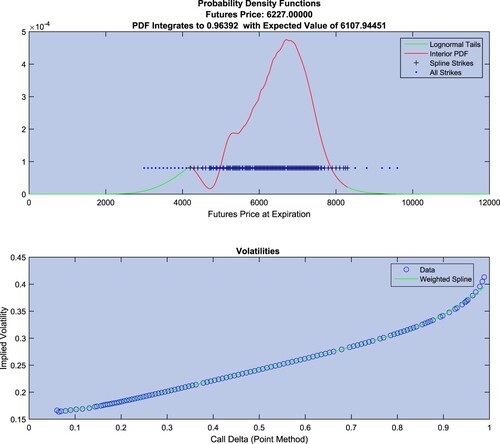
Figure 2 provides an example of the BP procedure for the same trading day as in figure 1. The only difference between the two figures are the left and right tails, as both the TailHAP and BP procedures follow the same method for producing the interior of the PDF. As can be seen in the heading for the top panel, the BP RND integrates to a value well below one and has a mean that is quite different from the futures price.

Figure 2. Top Panel: Example risk neutral density constructed using the Bliss and Panigirtzoglou (2002) estimation procedure. Bottom Panel: The spline fit in (call delta, implied volatility) space used in the construction of the interior of the risk neutral density shown in red in the top panel.

As figure 2 makes clear, the BP pasting of lognormal tails makes no attempt to match the left and right values of the RNCDF, that is, the BP procedure makes no attempt to ensure that the RND integrates to one. Therefore, we consider an alternative procedure, BPAlt, that adds lognormal tails that match both the RND and RNCDF at the attachment points by using fsolve to find the values for ${\mu }_L$, ${\sigma }_L,$ ${\mu }_R$, and ${\sigma }_R$ such that (33) $\begin{array}{rl}& \frac{1}{X_2\sqrt{2\pi }{\sigma }_L\sqrt{t}}{e}^{\left(\frac{-{(\ln \left(X_2\right)-{\mu }_L)}^2}{2{\sigma }_L^{2}t}\right)}=RND{}_2\\ & \mathrm{\Phi }\left(\frac{\ln \left(X_2\right)-{\mu }_L}{{\sigma }_L\sqrt{t}}\right)=RNCD{F}_2\\ & \frac{1}{X_{T-1}\sqrt{2\pi }{\sigma }_R\sqrt{t}}{e}^{\left(\frac{-{(\ln \left(X_{T-1}\right)-{\mu }_R)}^2}{2{\sigma }_R^{2}t}\right)}=RND{}_{T-1}\\ & \mathrm{\Phi }\left(\frac{\ln \left(X_{T-1}\right)-{\mu }_R}{{\sigma }_R\sqrt{t}}\right)=RNCD{F}_{T-1}\end{array}$(33)

4.3.3. FB construction

The construction of the interior of the RND in Figlewski (2010) and Birru and Figlewski (2012) uses a fourth order spline in $(X,\sigma )$ space with a single knot at the option price that is nearest to the money rather than the cubic spline in $({\mathrm{\Delta }}_i^{C_{point}},{\sigma }_i)$ space used in the TailHAP and BP procedures. We implement the fourth order spline using MatLab's spap2 routine. Not surprisingly, the different splining techniques produce different values for the interior portions of the RNCDF and RND, especially at the left end. On average, across all 1984 contract/trading days, the value for $RNCD{F}_2$ from the FB procedure is 27 percent below the value for $RNCD{F}_2$ from the TailHAP and BP procedures. The value for $RN{D}_2$ from the FB procedure averages 24 percent below the value for $RN{D}_2$ from the TailHAP and BP procedures.

The FB construction also differs in the functional form and attachment method of the left and right tails. The tails are both Generalized Extreme Value (GEV) distributions with parameters chosen to impose the constraints that the tails match the RND at two interior points and the RNCDF at one interior point. The GEV distribution and density are given by (34) $\begin{array}{rl}{f}_{GEV}\left(x\right)& =\{\begin{array}{ll}\begin{array}{l}{\displaystyle \frac{1}{\sigma }}{(1+\xi \left({\displaystyle \frac{x-\mu }{\sigma }}\right))}^{-1-1/\xi }\\ e^{-{(1+\xi \left(\frac{\mathrm{x}-\mu }{\sigma }\right))}^{-1/\xi }}\end{array}& \xi \ne 0\\ \frac{1}{\sigma }{e}^{-\left(\frac{x-\mu }{\sigma }\right)}\exp \left(-e^{-\left(\frac{x-\mu }{\sigma }\right)}\right)& \xi =0\end{array}\\ F_{GEV}\left(x\right)& =\{\begin{array}{ll}{e}^{-{(1+\xi \left(\frac{\mathrm{x}-\mu }{\sigma }\right))}^{-1/\xi }}& \xi \ne 0\\ \exp \left(-e^{-\left(\frac{x-\mu }{\sigma }\right)}\right)& \xi =0\end{array}x\in (-\mathrm{\infty },\mathrm{\infty })\end{array}$(34) Where possible, the FB methodology matches the right tail to the interior of the RND at the $X_i$ nearest the 92nd and 95th percentiles. Denoting these particular strikes by $X_{0.92}$ and $X_{0.95}$ and the heights of the RND at these points by $RN{D}_{0.92}$ and $RN{D}_{0.95}$, the right-tail parameters ${\mu }_R$, ${\sigma }_R$, and ${\xi }_R$ are solved for using the three conditions (35) $\begin{array}{rl}& F_{GEV}\left(X_{0.92}\right)=0.92\\ & f_{GEV}\left(X_{0.92}\right)=RND{}_{0.92}\\ & f_{GEV}\left(X_{0.95}\right)=RND{}_{0.95}\end{array}$(35) For the left tail, the FB methodology matches the interior of the RND at the $X_i$ nearest the 2nd and 5th percentile. Denoting these particular strikes by $X_{0.02}$ and $X_{0.05}$ and and the heights of the RND at these points by $RN{D}_{0.02}$ and $RN{D}_{0.05}$, the left-tail parameters ${\mu }_L$, ${\sigma }_L$, and ${\xi }_L$ are solved for. The left tail procedure is slightly more complicated than for the right tail. As explained by Figlewski ‘Since the GEV is the distribution of the maximum in a sample, its left tail relates to probabilities of small values of the maximum, rather than to extreme values of the sample minimum, i.e. the left tail. To adapt the GEV to fitting the left tail, we must reverse it left to right.’¹² Thus, the three conditions for the left tail are (36) $\begin{array}{rl}& F_{GEV}(-X_{0.05})=1-0.05\\ & f_{GEV}(-X_{0.05})=RND{}_{0.05}\\ & f_{GEV}(-X_{0.02})=RND{}_{0.02}\end{array}$(36) As mentioned in section 4.3, we only use options with call deltas within the range $[0.05,0.99]$, so the desired FB attachment points are rarely available in the interiors of the RNDs and RNCDFs. We then follow Figlewski (2010) and Birru and Figlewski (2012) when confronted with the same situation and implement the FB procedure by first finding the strike price with a RNCDF value as close as possible to $RNCD{F}_{T-1}-0.03$, denoted $X_{\alpha 0R}$, and the strike price with a RNCDF value as close as possible to $RNCD{F}_2+0.03,$ denoted $X_{\alpha 0L}$. In these cases, the FB tails are constructed so that (37) $\begin{array}{rl}& F_{GEV}\left(X_{\alpha 0R}\right)=RNCD{F}_{X_{\alpha 0R}}\\ & f_{GEV}\left(X_{\alpha 0R}\right)=RND{}_{X_{\alpha 0R}}\\ & f_{GEV}\left(X_{T-1}\right)=RND{}_{T-1}\end{array}$(37) and (38) $\begin{array}{rl}& F_{GEV}(-X_{\alpha 0L})=1-RNCD{F}_{X_{\alpha 0L}}\\ & f_{GEV}(-X_{\alpha 0L})=RND{}_{X_{\alpha 0L}}\\ & f_{GEV}(-X_2)=RND{}_2\end{array}$(38) F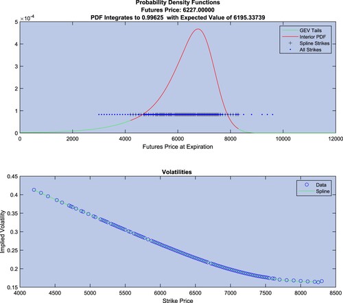igure 3 shows that on the same example day the FB procedure produces a much smoother interior for the RND - a result that also holds in general. The bottom panel shows the FB spline in $(X,\sigma )$ space. The header for the top panel demonstrates that the FB procedure produces a RND with an integral essentially equal to one. However, the expected value for the RND is not as close to the futures price as for the TailHAP procedure. We return to this point in section 5.

Figure 3. Top Panel: Example risk neutral density constructed using the Birru and Figlewski (2012) estimation procedure. Bottom Panel: The spline fit in (strike price, implied volatility) space used in the construction of the interior of the risk neutral density shown in red in the top panel.

5. RND evaluation

Applying the five procedures in section 4.3 to our FTSE 100 data generates five sets of 2850 constructed RNDs and five sets of 381 696 estimated option prices. Evaluation of these results can be conducted both at the level of the RND and at the level of option prices, with the latter including assessment across maturity, moneyness, and sample. Prior to this evaluation, attention must be paid to the definitions of options that are in and out of sample.

5.1. Option sample definitions

When dealing with option pricing, the difference between in and out of sample is not clear cut if Put-Call Parity holds. Applying the bottom half of equation (10(10) $\begin{array}{rl}{P}_1& =e^{-rt}max((X_1-E[F_T\mid F_T<X_1])Pr[F_T<X_1],0)\\ & =e^{-rt}(X_1-\frac{{\int }_0^{X_1}{F}_T{f}_L\left(F_T\right)\mathrm{d}{F}_T}{{\int }_0^{X_1}{f}_L\left(F_T\right)\mathrm{d}{F}_T}){\int }_0^{X_1}{f}_L\left(F_T\right)\mathrm{d}{F}_T\\ & =e^{-rt}{\int }_0^{X_1}(X_1-F_T)f_L\left(F_T\right)\mathrm{d}{F}_T\mathrm{a}\mathrm{n}\mathrm{d}\\ C_N& =e^{-rt}max((E[F_T\mid F_T>X_T]-X_T)Pr[F_T>X_T],0)\\ & =e^{-rt}(\frac{{\int }_{X_T}^{\mathrm{\infty }}{F}_T{f}_R\left(F_T\right)\mathrm{d}{F}_T}{{\int }_{X_T}^{\mathrm{\infty }}{f}_R\left(F_T\right)\mathrm{d}{F}_T}-X_T){\int }_{X_T}^{\mathrm{\infty }}{f}_R\left(F_T\right)\mathrm{d}{F}_T\\ & =e^{-rt}{\int }_{X_T}^{\mathrm{\infty }}(F_T-X_T)f_R\left(F_T\right)\mathrm{d}{F}_T\end{array}$(10) ) to the case of pricing a call option with strike X written on a futures contract the price of which at expiration will be drawn from the RND $f\left(F_T\right)$ we have (39) $\begin{array}{rl}C& =e^{-rt}{\int }_X^{\mathrm{\infty }}(F_T-X)f\left(F_T\right)\mathrm{d}{F}_T\\ & =e^{-rt}({\int }_X^{\mathrm{\infty }}{F}_{T}f\left(F_T\right)\mathrm{d}{F}_T-X{\int }_X^{\mathrm{\infty }}f\left(F_T\right)\mathrm{d}{F}_T)\end{array}$(39) A valid RND will integrate to 1.0 and, in the case of futures, will have a mean equal to $F_t$ (the current futures price). (40) $\begin{array}{rl}& {\int }_0^{X}f\left(F_T\right)\mathrm{d}{F}_T+{\int }_X^{\mathrm{\infty }}f\left(F_T\right)\mathrm{d}{F}_T=1\mathrm{a}\mathrm{n}\mathrm{d}\\ & {\int }_0^X{F}_{T}f\left(F_T\right)\mathrm{d}{F}_T+{\int }_X^{\mathrm{\infty }}{F}_{T}f\left(F_T\right)\mathrm{d}{F}_T=F_t\end{array}$(40) Substituting results from equation (40(40) $\begin{array}{rl}& {\int }_0^{X}f\left(F_T\right)\mathrm{d}{F}_T+{\int }_X^{\mathrm{\infty }}f\left(F_T\right)\mathrm{d}{F}_T=1\mathrm{a}\mathrm{n}\mathrm{d}\\ & {\int }_0^X{F}_{T}f\left(F_T\right)\mathrm{d}{F}_T+{\int }_X^{\mathrm{\infty }}{F}_{T}f\left(F_T\right)\mathrm{d}{F}_T=F_t\end{array}$(40) ) into equation (39(39) $\begin{array}{rl}C& =e^{-rt}{\int }_X^{\mathrm{\infty }}(F_T-X)f\left(F_T\right)\mathrm{d}{F}_T\\ & =e^{-rt}({\int }_X^{\mathrm{\infty }}{F}_{T}f\left(F_T\right)\mathrm{d}{F}_T-X{\int }_X^{\mathrm{\infty }}f\left(F_T\right)\mathrm{d}{F}_T)\end{array}$(39) ) and comparing to equation (10(10) $\begin{array}{rl}{P}_1& =e^{-rt}max((X_1-E[F_T\mid F_T<X_1])Pr[F_T<X_1],0)\\ & =e^{-rt}(X_1-\frac{{\int }_0^{X_1}{F}_T{f}_L\left(F_T\right)\mathrm{d}{F}_T}{{\int }_0^{X_1}{f}_L\left(F_T\right)\mathrm{d}{F}_T}){\int }_0^{X_1}{f}_L\left(F_T\right)\mathrm{d}{F}_T\\ & =e^{-rt}{\int }_0^{X_1}(X_1-F_T)f_L\left(F_T\right)\mathrm{d}{F}_T\mathrm{a}\mathrm{n}\mathrm{d}\\ C_N& =e^{-rt}max((E[F_T\mid F_T>X_T]-X_T)Pr[F_T>X_T],0)\\ & =e^{-rt}(\frac{{\int }_{X_T}^{\mathrm{\infty }}{F}_T{f}_R\left(F_T\right)\mathrm{d}{F}_T}{{\int }_{X_T}^{\mathrm{\infty }}{f}_R\left(F_T\right)\mathrm{d}{F}_T}-X_T){\int }_{X_T}^{\mathrm{\infty }}{f}_R\left(F_T\right)\mathrm{d}{F}_T\\ & =e^{-rt}{\int }_{X_T}^{\mathrm{\infty }}(F_T-X_T)f_R\left(F_T\right)\mathrm{d}{F}_T\end{array}$(10) ) yields the familiar Put-Call Parity equation for options on futures. (41) $\begin{array}{rl}C& =e^{-rt}(F_t-{\int }_0^X{F}_{T}f\left(F_T\right)\mathrm{d}{F}_T\\ & -X(1-{\int }_0^{X}f\left(F_T\right)\mathrm{d}{F}_T))\\ & =e^{-rt}(X{\int }_0^{X}f\left(F_T\right)\mathrm{d}{F}_T-{\int }_0^X{F}_{T}f\left(F_T\right)\mathrm{d}{F}_T)\\ & +e^{-rt}(F_t-X)\\ & =P+e^{-rt}(F_t-X)\end{array}$(41) Thus, if we calculate the difference between an observed option price C and a predicted option price $\hat{C}$ from a constructed RND and Put-Call Parity holds for both the actual and predicted prices we find that a put and a call that share the same strike price will also share the identical pricing error. (42) $C-\hat{C}=P+e^{-rt}(F_t-X)-(\hat{P}+e^{-rt}(F_t-X))=P-\hat{P}$(42) Obviously, the OTM options used to create the RND (the left hand side of equation (1(1) $\begin{array}{rl}& \left[\begin{array}{cc}{K}_1& P_1\\ K_2& P_2\\ ..& ..\\ K_{N-1}& C_{N-1}\\ K_N& C_N\end{array}\right]\\ & ⟹\left[\begin{array}{cccc}{X}_1& \widehat{C_1}& .& .\\ X_2& \widehat{C_2}& RNCD{F}_2& RN{D}_2\\ X_3& \widehat{C_3}& RNCD{F}_3& RN{D}_3\\ ..& ..& ..& ..\\ X_{T-2}& \widehat{C_{T-2}}& RNCD{F}_{T-2}& RN{D}_{T-2}\\ X_{T-1}& \widehat{C_{T-1}}& RNCD{F}_{T-1}& RN{D}_{T-1}\\ X_T& \widehat{C_T}& .& .\end{array}\right]\end{array}$(1) )) are definitely in sample options. However, any in the money (ITM) options that share the same strike with an OTM option will also share the exact same pricing error and therefore are not truly out of sample. For this reason we divide our options prices into three, non-overlapping categories: In Sample, Out of Sample, and Quasi Out of Sample. In Sample options are those on the left hand side of equation (1(1) $\begin{array}{rl}& \left[\begin{array}{cc}{K}_1& P_1\\ K_2& P_2\\ ..& ..\\ K_{N-1}& C_{N-1}\\ K_N& C_N\end{array}\right]\\ & ⟹\left[\begin{array}{cccc}{X}_1& \widehat{C_1}& .& .\\ X_2& \widehat{C_2}& RNCD{F}_2& RN{D}_2\\ X_3& \widehat{C_3}& RNCD{F}_3& RN{D}_3\\ ..& ..& ..& ..\\ X_{T-2}& \widehat{C_{T-2}}& RNCD{F}_{T-2}& RN{D}_{T-2}\\ X_{T-1}& \widehat{C_{T-1}}& RNCD{F}_{T-1}& RN{D}_{T-1}\\ X_T& \widehat{C_T}& .& .\end{array}\right]\end{array}$(1) ). Out of Sample options are any options that are not In Sample and do not share a strike with any of the In Sample options. Quasi Out of Sample options are the those options that are not In Sample but share a strike with one of the In Sample options.

5.2. RND characteristics

Ideally the constructed RNDs would integrate to 1.0 and have a mean equal to the prevailing futures price. Calculating these integrals for the constructed RNDs is somewhat complicated by their blended nature—left and right tails attached to an interior. Given that the FTSE 100 Index is based on share prices, the theoretical support of the RND is $[0,\mathrm{\infty })$ but we obtain our results by numerically integrating the integrals in equations (9(9) $\begin{array}{rl}& {\int }_0^{X_2}{f}_L\left(F_T\right)\mathrm{d}{F}_T+\sum _{j=2}^{T-1}(X_j-X_{j-1})RND{}_j\\ & +{\int }_{X_{T-1}}^{\mathrm{\infty }}{f}_R\left(F_T\right)\mathrm{d}{F}_T=1\end{array}$(9) ) and (11(11) $\begin{array}{rl}& {\int }_0^{X_2}{F}_T{f}_L\left(F_T\right)\mathrm{d}{F}_T+\sum _{j=2}^{T-1}{X}_j(X_j-X_{j-1})RN{D}_j\\ & +{\int }_{X_{T-1}}^{\mathrm{\infty }}{F}_T{f}_R\left(F_T\right)\mathrm{d}{F}_T=F\end{array}$(11) ) over the support $[0,1,2,\dots 12000]$ using MatLab's trapz function. This interval appears to be wide enough as the tails of the RND typically fall off quite quickly.

As can be seen in the top third of table 5, most of the procedures produce RNDs with integrals that are quite close to 1.0 as most of the procedures attempt to match the values from the interior of the RND at the attachment points. Unsurprisingly, the BP procedure is the lone exception as it makes no attempt to match the values of interior RND, typically resulting in an integral that is less than 1.0. On rare occasions, the FB procedure produces a RND that integrates to well below 1.0. This is likely due to using a GEV density for the tails. As seen in equation (34(34) $\begin{array}{rl}{f}_{GEV}\left(x\right)& =\{\begin{array}{ll}\begin{array}{l}{\displaystyle \frac{1}{\sigma }}{(1+\xi \left({\displaystyle \frac{x-\mu }{\sigma }}\right))}^{-1-1/\xi }\\ e^{-{(1+\xi \left(\frac{\mathrm{x}-\mu }{\sigma }\right))}^{-1/\xi }}\end{array}& \xi \ne 0\\ \frac{1}{\sigma }{e}^{-\left(\frac{x-\mu }{\sigma }\right)}\exp \left(-e^{-\left(\frac{x-\mu }{\sigma }\right)}\right)& \xi =0\end{array}\\ F_{GEV}\left(x\right)& =\{\begin{array}{ll}{e}^{-{(1+\xi \left(\frac{\mathrm{x}-\mu }{\sigma }\right))}^{-1/\xi }}& \xi \ne 0\\ \exp \left(-e^{-\left(\frac{x-\mu }{\sigma }\right)}\right)& \xi =0\end{array}x\in (-\mathrm{\infty },\mathrm{\infty })\end{array}$(34) ), the support for the GEV density is $(-\mathrm{\infty },\mathrm{\infty })$ whereas our numerical integrals only use the range $[0,12000]$. If the estimated GEV tail parameters leave some probability mass below zero, then the resulting integral calculated over the $[0,12000]$ range will be less than 1.0.

Table 5. Risk neutral density performance across the five alternate estimation procedures for the 2850 trading days in the sample. Performance is measured in terms of: the density integrating to 1.0, the difference between the expected value of the density and the futures price for the particular contract on the trading day, the square percent error in matching the probability mass in the left and right tails, and the difference between the predicted option price and the actual option price at the attachment point. RMSE and RMSPE denote root mean square error and root mean square percent error.

	Procedure
	TailHAP	TailHAPAlt	BP	BPAlt	FB
Integral of the RND
Mean	1.000	1.000	0.968	1.000	0.997
Minimum value	0.949	0.986	0.822	1.000	0.811
Maximum value	1.014	1.014	1.117	1.000	1.007
E[RND] - Futures
Mean	−3.731	−3.325	−117.089	−14.942	−24.699
Minimum value	−359.755	−15.283	−505.044	−165.656	−708.526
Maximum value	68.615	142.592	1693.421	126.659	93.124
RMSE	11.389	14.792	193.215	26.675	39.076
Left CDF Square Percent Error
Mean	0.001	0.001	0.202	0.000	0.000
RMSPE	0.029	0.029	0.450	0.000	0.004
Right CDF Square Percent Error
Mean	0.000	0.000	0.001	0.000	0.000
RMSPE	0.001	0.000	0.030	0.000	0.001
Left Option Pricing Error (Predicted - Actual)
Mean	−0.000	0.000	−32.492	9.069	5.544
RMSE	0.000	0.000	48.704	23.127	10.139
Right Option Pricing Error (Predicted - Actual)
Mean	0.004	2.556	5.872	0.452	−3.261
RMSE	0.168	22.288	35.409	6.376	6.310

All of the procedures produce RNDs with expected values that, on average, are less than the prevailing FTSE 100 Index futures price. In terms of RMSE, the TailHAP procedure comes closest to the futures price, followed by TailHAPAlt. Again unsurprisingly, the BP procedure struggles in this regard because it does not attempt to incorporate any information from the interior RNCDF in its construction, thereby generating an expected value that is typically quite far below the futures price.

The bottom two-thirds of table 5 provide measures of how well the tails of the constructed RNDs match the attachment point values of the RND and the observed option prices at $X_1$ and $X_N$. For the TailHAP and TailHAPAlt procedures, this information simply shows that these conditions are generally satisfied, subject to the limitations of the fsolve routine, as they were used as constraints in the construction of the RND. The same is true for the left and right CDF errors for the FB procedures. For the BP procedure, ignoring the values for the interior RND leads to large discrepancies for the mass in the left tail vis-a-vis the interior RNCDF but almost no discrepancies for the mass in the right tail. Looking across all the entries in table 5, the TailHAP procedure generates RNDs that come closest to the ideal characteristics.

5.3. Option pricing errors

Our emphasis on the ability of the RND to accurately price options is shared by Reinke (2020) who compares the RND techniques of Figlewski (2010) and Jackwerth (2004) using options on the S&P 500 Index. As in Reinke (2020), we use root mean square error (RMSE) as our measure of accuracy when calculating pricing errors. Unlike Reinke, we do not emphasize errors calculated in terms of implied volatilities. Using implied volatilities is certainly reasonable given that option traders routinely quote prices in terms of implied volatilities. However, when deciding whether or not a pricing error is large or small, expressing the pricing error in terms of the fundamental units in which contracts are settled (pounds sterling in the case of the FTSE 100) provides a more intuitive measure of the RND's accuracy. An option mispricing of 0.1 implied volatility percentage points is not as easily interpretable as a mispricing of £15 that can be compared to the transactions cost of taking positions to profit from the mispricing.

The LIFFE options on the FTSE 100 are quoted in FTSE 100 index points, with each index point equal to £10. All of our pricing errors are reported in pounds sterling by multiplying the index point difference between the predicted and actual option price by £10. We obtain the pricing errors by numerically integrating the integrals similar to those in equation (10(10) $\begin{array}{rl}{P}_1& =e^{-rt}max((X_1-E[F_T\mid F_T<X_1])Pr[F_T<X_1],0)\\ & =e^{-rt}(X_1-\frac{{\int }_0^{X_1}{F}_T{f}_L\left(F_T\right)\mathrm{d}{F}_T}{{\int }_0^{X_1}{f}_L\left(F_T\right)\mathrm{d}{F}_T}){\int }_0^{X_1}{f}_L\left(F_T\right)\mathrm{d}{F}_T\\ & =e^{-rt}{\int }_0^{X_1}(X_1-F_T)f_L\left(F_T\right)\mathrm{d}{F}_T\mathrm{a}\mathrm{n}\mathrm{d}\\ C_N& =e^{-rt}max((E[F_T\mid F_T>X_T]-X_T)Pr[F_T>X_T],0)\\ & =e^{-rt}(\frac{{\int }_{X_T}^{\mathrm{\infty }}{F}_T{f}_R\left(F_T\right)\mathrm{d}{F}_T}{{\int }_{X_T}^{\mathrm{\infty }}{f}_R\left(F_T\right)\mathrm{d}{F}_T}-X_T){\int }_{X_T}^{\mathrm{\infty }}{f}_R\left(F_T\right)\mathrm{d}{F}_T\\ & =e^{-rt}{\int }_{X_T}^{\mathrm{\infty }}(F_T-X_T)f_R\left(F_T\right)\mathrm{d}{F}_T\end{array}$(10) ) over the support $[0,1,2,\dots 12000]$ using MatLab's trapz function.

Table 6 presents statistics on overall pricing errors for each of the procedures. Given that our option prices cover a wide range from 0.5 to 4791 FTSE 100 Index points, we present pound pricing errors in both level and percentage terms. The mean values indicate whether the average error is an under or over pricing of the option. For three out of the five procedures, the options are generally overpriced, a point that we return to shortly in the discussion of table 7.

Table 6. Descriptive statistics for option pricing errors (Predicted - Actual) for all 381 696 options in the dataset across the five risk neutral density estimation procedures in terms of: British pounds, British pound pricing errors in percentage terms, and implied volatility. RMSE and RMSPE denote root mean square error and root mean square percent error.

	Procedure
	TailHAP	TailHAPAlt	BP	BPAlt	FB
Pound Pricing Errors
Mean	15.890	19.076	−379.013	60.552	−15.029
RMSE	67.569	108.337	895.985	185.769	147.489
Pound Percent Pricing Errors
Mean	−3.725	−3.937	−18.944	−1.328	1.927
RMSPE	20.124	21.000	36.306	20.476	30.268
Volatility Pricing Errors
Mean	−0.015	−0.017	−0.062	−0.013	−0.012
RMSE	0.081	0.085	0.118	0.088	0.078

Table 7. Descriptive statistics for put and call option pricing errors in British pounds (Predicted - Actual) for all 381 696 options in the dataset across the five risk neutral density estimation procedures. RMSE and RMSPE denote root mean square error and root mean square percent error.

	Procedure
	TailHAP	TailHAPAlt	BP	BPAlt	FB
Puts
Mean	48.399	47.921	−796.820	141.802	14.512
RMSE	78.051	78.208	1167.085	247.969	196.079
Calls
Mean	−17.527	−10.576	50.474	−22.969	−45.395
RMSE	54.741	132.342	477.341	82.322	67.765

The RMSE provides the best sense of the magnitude of errors. For example, the TailHAP procedure produces an average mispricing of roughly £68 or 6.8 FTSE 100 Index points, or almost 14 ticks. Such an error is large if market participants can take positions to profit from the mispricing of these options for less than roughly £70. We also tabulate percent pricing errors, given that an error of 5 FTSE 100 Index points is quite small for an option with an observed price of 1000 index points but quite large for an observed option with a price of 6 index points. Using this metric across all five procedures, TailHAP provides the best pricing performance, but not always by a wide margin. The TailHAPt and BPAlt procedures produce percent errors that are only slightly larger. Given its lack of attention to interior RNCDF values, the BP procedure suffers from relatively large RMSE pricing errors both in pound and percentage terms.

The bottom panel of table 6 shows errors in terms of implied volatility by comparing each option's implied volatility recovered from equation (2(2) $\begin{array}{rl}C\left(K_i\right)& =e^{-rt}(F\mathrm{\Phi }\left(d_{1,i}\right)-K_i\mathrm{\Phi }\left(d_{2,i}\right))\mathrm{a}\mathrm{n}\mathrm{d}\\ P\left(K_i\right)& =e^{-rt}(K_i\mathrm{\Phi }\left(-d_{2,i}\right)-F\mathrm{\Phi }\left(-d_{1,i}\right))\\ d_{1,i}& =\frac{\ln \left(\frac{F}{K_i}\right)+\frac{{\sigma }_i^{2}t}{2}}{{\sigma }_i\sqrt{t}}\mathrm{a}\mathrm{n}\mathrm{d}{d}_{2,i}=d_{1,i}-{\sigma }_i\sqrt{t}\end{array}$(2) ) with the implied volatility for the predicted option price from the RND. This panel allows for only a very rough comparison with Reinke's S&P 500 Index options results. Our calculations are across all 381 696 options in the sample, whereas Reinke calculates RMSE for each trading day. All five of our procedures understate implied volatility on average. In terms of RMSE volatility errors, FB has the best performance, followed closely by TailHAP and TailHAPAlt. Reinke reports average in and out of sample RMSEs across 1537 trading days for the equivalent of our FB procedure that range from 0.0176 to 0.0486 for calls and 0.1059 to 0.1673 for puts - not terribly different from the values reported in the bottom panel of table 6.

Errors can also be examined across option type, maturity, moneyness, and sample. Table 7 presents pricing errors separately for puts and calls, omitting percent pricing errors. Aside from the extremely large errors for the BP procedure, pricing errors for puts are positive (the puts are overpriced) and negative for the calls (the calls are underpriced). Because puts pay off in the event that the underlying asset price falls below the strike price, put prices are largely determined by the left side of the RND. Call prices, where the option pays off in the event that the underlying price exceeds the strike price, are largely determined by the right side of the RND. Thus, table 7 suggests that all but the BP procedure are producing RNDs with left sides that contain too much probability mass (‘fat’ left sides) and right sides that contain too little probability mass (‘thin’ right sides). More detailed tables of put and call errors across moneyness and sample indicate that puts are generally overpriced across every type of option except for deep out of the money puts that are also out of sample.¹³ The underpricing of calls is largely the result of large underpricing errors for deep in the money calls whether they are out of sample or quasi out of sample. In short, puts are overpriced except for those with very low strikes that are out of sample. Thus, the fat left side of the RND is not exclusively the result of a fat far-left tail. Call underpricing is most pronounced for those calls with very low strike prices - also the result of a fat left side of the RND. The smaller put option RMSEs for the TailHAP and TailHAPAlt procedures seen in the second row of table 7 are evidence in favor of our methodology that matches the option price with strike $K_1=X_1$ when fitting the left tail.

Errors by maturity are found in table 8. Here, the TailHAP and TailHAPAlt procedures generally have only a slightly better performance than the FB procedure at short maturities, but the advantage widens at longer maturities with the notable exception of relatively large errors for TailHAPAlt for options with greater than 300 days to maturity. As can be seen in table 9, the TailHAP procedure produces the smallest RMSEs across all the moneyness categories, most notably for the ATM and ITM categories. The TailHAPAlt procedure is generally a close second.

Table 8. Descriptive statistics for option pricing errors in British pounds (Predicted - Actual) by days to expiration for all 381 696 options in the dataset across the five risk neutral density estimation procedures. RMSE denotes root mean square error.

	Procedure
	TailHAP	TailHAPAlt	BP	BPAlt	FB
Days to Expiration Less than 60
Mean	4.041	2.979	−159.655	7.601	14.002
RMSE	41.573	36.181	296.550	46.885	46.768
Between 60 and 120
Mean	9.333	6.820	−289.374	29.926	15.043
RMSE	53.512	55.934	529.305	96.803	59.787
Between 120 and 180
Mean	14.287	10.978	−366.906	44.026	4.582
RMSE	63.874	66.780	665.959	126.620	61.250
Between 180 and 240
Mean	17.974	15.360	−478.238	75.504	−13.997
RMSE	70.000	72.360	933.582	211.633	73.634
Between 240 and 300
Mean	23.122	22.338	−544.137	98.850	-59.214
RMSE	77.883	81.224	1214.997	257.186	326.237
Greater Than 300
Mean	29.984	67.320	−454.675	124.355	−69.952
RMSE	93.527	245.665	1418.473	289.069	148.489

Table 9. Descriptive statistics for option pricing errors in British pounds (Predicted - Actual) by moneyness for all 381 696 options in the dataset across the five risk neutral density estimation procedures. OTM denotes out of the money, ATM denotes at the money, ITM denotes in the money, and RMSE denotes root mean square error.

	Procedure
	TailHAP	TailHAPAlt	BP	BPAlt	FB
Deep OTM
Mean	−14.055	−15.803	−150.195	21.794	47.256
RMSE	58.210	60.993	213.346	92.512	69.861
OTM
Mean	42.409	42.097	−282.448	96.592	8.782
RMSE	61.315	63.256	521.731	203.270	67.055
ATM
Mean	38.657	52.293	−443.040	108.218	−29.659
RMSE	59.855	154.652	1077.453	232.460	166.816
ITM
Mean	32.594	34.259	−530.839	77.945	−37.298
RMSE	55.695	81.622	1213.037	177.014	195.209
Deep ITM
Mean	−44.131	−49.918	−412.565	−47.224	−46.925
RMSE	99.157	103.842	835.804	137.942	164.678

Finally, and perhaps most interestingly, table 10 presents pricing errors by sample for each of the procedures. For in sample options, the TailHAP procedure returns the smallest RMSE. The out of sample results present the most stringent pricing criterion - how well do the constructed RNDs price options that played no part in the construction of the RND? Here again, the TailHAP procedure has the smallest RMSE, and by a wide margin. The same is true for the quasi out of sample options.

Table 10. Descriptive statistics for option pricing errors in British pounds (Predicted - Actual) by sample for all 381 696 options in the dataset across the five risk neutral density estimation procedures. In sample options are those used to construct the interior of the risk neutral density. Out of sample options are those options that were not used to construct the interior of the risk neutral density and that do not share a strike with an option used to construct the interior. Quasi out of sample options are the remaining options - those options that share a strike with an in sample option. RMSE denotes root mean square error.

	Procedure
	TailHAP	TailHAPAlt	BP	BPAlt	FB
In Sample
Mean	41.034	45.449	−319.822	100.136	2.466
RMSE	59.942	103.382	695.088	208.154	96.479
Out of Sample
Mean	−29.650	−30.311	−288.356	−0.660	12.400
RMSE	64.102	86.992	848.568	104.733	228.378
Quasi Out of Sample
Mean	9.793	13.228	−460.451	47.399	−39.314
RMSE	74.522	118.529	1051.016	186.917	148.678

6. Conclusion

We demonstrate the viability of adding additional constraints when attaching the tails to the interior of a constructed RND. In particular, we document the feasibility of ensuring that the left and right tails correctly price the observed option prices at the attachment points, using either a Weibull (TailHAP) or lognormal (TailHAPAlt) functional form for the tails. We recognize that these pricing constraints, especially for the Weibull functional form, increase the numerical complexity of the RND construction. For the Weibull (TailHAP) choice, care must be taken in selecting the starting values as detailed in the Appendix. Finding the best starting values requires some patience, and even with good starting values the TailHAP procedure requires roughly twice as much computing time than does the TailHAPAlt procedure. Is the additional complexity worth the cost? We think so, based on the generally superior performance of the TailHAP procedure documented in section 5. The TailHAP procedure does best both in terms of the characteristics of the RND and the pricing of individual options. For those wishing to minimize these numerical issues, the TailHAPAlt or FB procedures may be preferred.

The advantage of the TailHAP procedure is not merely the result of using the flexible functional form of the Weibull distribution for the tails. The Weibull itself is a special case of the GEV distribution used in the FB procedure. Rather, the advantage of the TailHAP procedure stems from incorporating the information in the attachment point option prices on the location, and not just the amount, of the probability mass in the left and right tails. Even using the less flexible function form of the lognormal distribution in the TailHAPAlt procedure still results in a generally superior performance compared to the methods that do not attempt to match the prices of the options at the attachment points.

We reach several other conclusions. First, for almost all of the procedures the estimated RNDs generally overprice puts and underprice calls. Second, attaching tails without regard to values from the interior RNCDF (BP procedure) produces quite large errors that can be dramatically reduced with relatively little effort (BPAlt). Third, in a few instances the $(-\mathrm{\infty },\mathrm{\infty })$ support of the GEV creates problems for the FB procedure to return a RND that integrates to one, has a mean that matches the futures price, and accurately prices put options. On the other hand, the FB procedure produces a very smooth interior RND. Practitioners should be aware of these trade-offs. Finally, we document that Put-Call Parity complicates the determination of which options are in and out of sample in the construction of a RND.

Acknowledgments

For helpful comments we are indebted to Martin Reinke and three anonymous referees.

Disclosure statement

No potential conflict of interest was reported by the author(s).

Notes

1 See Markose and Alentorn (2011) for a graphical representation of one such classification system.

2 More details can be found below in section 4.3.2.

3 Although they do not make any explicit comparisons with curve-fitting results, Cui and Xu (2022) also call attention to the popularity of curve-fitting techniques when introducing a new RND estimation technique based on the spanning result of Carr and Madan (1999).

4 The point conversion method is used to ensure that the order of the options in strike price - option price space will be preserved when converted into call delta - sigma space.

5 See also Savickas (2005) for additional option pricing applications of the Weibull distribution.

6 The WRDS subscription does not allow access to the most recent year's data.

7 In their applications to FTSE 100 options, Bliss and Panigirtzoglou (2004) and Markose and Alentorn (2011) also use GBP LIBOR rates.

8 See McDonald (2012).

9 In MatLab $L\simeq -38.381$ and $H\simeq 7.65$.

10 available at https://www.jefferson-duarte.com.

11 Bliss and Panigirtzoglou (2004) page 417.

12 Figlewski (2010) page 343.

13 These detailed tables are available from the authors upon request.

14 Using a GEV distribution to price the options also involves $\gamma (z,M)$ and $\mathrm{\Gamma }(z,M)$ as can be seen by replacing the Weibull distribution in equations (14(14) $f_L\left(F_T\right)={\text{β}}_L\frac{k_L}{{\lambda }_L}{\left(\frac{F_T}{{\lambda }_L}\right)}^{k_L-1}{e}^{-{\left(\frac{F_T}{{\lambda }_L}\right)}^{k_L}}\mathrm{w}\mathrm{h}\mathrm{e}\mathrm{r}\mathrm{e}{\text{β}}_L=\frac{RN{D}_2}{f_L\left(X_2\right)}$(14) ) and (20(20) $\begin{array}{rl}& f_R\left(F_T\right)={\text{β}}_R\frac{k_R}{{\lambda }_R}{\left(\frac{F_T}{{\lambda }_R}\right)}^{k_R-1}{e}^{-{\left(\frac{F_T}{{\lambda }_R}\right)}^{k_R}}\mathrm{w}\mathrm{h}\mathrm{e}\mathrm{r}\mathrm{e}\\ & {\text{β}}_R=\frac{RN{D}_{T-1}}{f_R\left(X_{T-1}\right)}\end{array}$(20) ) with the GEV distribution and proceeding with the pricing solutions. See also Markose and Alentorn (2011).

Appendix

TailHAP starting values

As made clear in sections 3.2.1 and 3.2.2, using the Weibull distribution to price options involves the lower and upper incomplete gamma functions $\gamma (z,M)$ and $\mathrm{\Gamma }(z,M)$.¹⁴ These functions can create problems for non-linear equation solvers such as MatLab's fsolve, as the solver can easily select parameter values such that either z<0 and/or $M\in \mathbb{C}$ at which point the incomplete gamma functions cannot be evaluated and the solver fails. For this reason, high-quality starting values are critical in implementing the TailHAP procedure.

To determine these starting values, we first start with a simpler problem involving the lognormal density function. As is made clear in equation (10(10) $\begin{array}{rl}{P}_1& =e^{-rt}max((X_1-E[F_T\mid F_T<X_1])Pr[F_T<X_1],0)\\ & =e^{-rt}(X_1-\frac{{\int }_0^{X_1}{F}_T{f}_L\left(F_T\right)\mathrm{d}{F}_T}{{\int }_0^{X_1}{f}_L\left(F_T\right)\mathrm{d}{F}_T}){\int }_0^{X_1}{f}_L\left(F_T\right)\mathrm{d}{F}_T\\ & =e^{-rt}{\int }_0^{X_1}(X_1-F_T)f_L\left(F_T\right)\mathrm{d}{F}_T\mathrm{a}\mathrm{n}\mathrm{d}\\ C_N& =e^{-rt}max((E[F_T\mid F_T>X_T]-X_T)Pr[F_T>X_T],0)\\ & =e^{-rt}(\frac{{\int }_{X_T}^{\mathrm{\infty }}{F}_T{f}_R\left(F_T\right)\mathrm{d}{F}_T}{{\int }_{X_T}^{\mathrm{\infty }}{f}_R\left(F_T\right)\mathrm{d}{F}_T}-X_T){\int }_{X_T}^{\mathrm{\infty }}{f}_R\left(F_T\right)\mathrm{d}{F}_T\\ & =e^{-rt}{\int }_{X_T}^{\mathrm{\infty }}(F_T-X_T)f_R\left(F_T\right)\mathrm{d}{F}_T\end{array}$(10) ), put and call option prices with strikes at the observed option prices with the lowest and highest strikes are partly determined by the conditional expectations for the price of the underlying asset: $E[F_T\mid F_T<X_1]$ and $E[F_T\mid F_T>X_T]$. If the RND for the price of the underlying asset was a lognormal density, as assumed in the Black model, then it is not difficult to calculate these conditional expectations. By comparing equations (2(2) $\begin{array}{rl}C\left(K_i\right)& =e^{-rt}(F\mathrm{\Phi }\left(d_{1,i}\right)-K_i\mathrm{\Phi }\left(d_{2,i}\right))\mathrm{a}\mathrm{n}\mathrm{d}\\ P\left(K_i\right)& =e^{-rt}(K_i\mathrm{\Phi }\left(-d_{2,i}\right)-F\mathrm{\Phi }\left(-d_{1,i}\right))\\ d_{1,i}& =\frac{\ln \left(\frac{F}{K_i}\right)+\frac{{\sigma }_i^{2}t}{2}}{{\sigma }_i\sqrt{t}}\mathrm{a}\mathrm{n}\mathrm{d}{d}_{2,i}=d_{1,i}-{\sigma }_i\sqrt{t}\end{array}$(2) ) and (10(10) $\begin{array}{rl}{P}_1& =e^{-rt}max((X_1-E[F_T\mid F_T<X_1])Pr[F_T<X_1],0)\\ & =e^{-rt}(X_1-\frac{{\int }_0^{X_1}{F}_T{f}_L\left(F_T\right)\mathrm{d}{F}_T}{{\int }_0^{X_1}{f}_L\left(F_T\right)\mathrm{d}{F}_T}){\int }_0^{X_1}{f}_L\left(F_T\right)\mathrm{d}{F}_T\\ & =e^{-rt}{\int }_0^{X_1}(X_1-F_T)f_L\left(F_T\right)\mathrm{d}{F}_T\mathrm{a}\mathrm{n}\mathrm{d}\\ C_N& =e^{-rt}max((E[F_T\mid F_T>X_T]-X_T)Pr[F_T>X_T],0)\\ & =e^{-rt}(\frac{{\int }_{X_T}^{\mathrm{\infty }}{F}_T{f}_R\left(F_T\right)\mathrm{d}{F}_T}{{\int }_{X_T}^{\mathrm{\infty }}{f}_R\left(F_T\right)\mathrm{d}{F}_T}-X_T){\int }_{X_T}^{\mathrm{\infty }}{f}_R\left(F_T\right)\mathrm{d}{F}_T\\ & =e^{-rt}{\int }_{X_T}^{\mathrm{\infty }}(F_T-X_T)f_R\left(F_T\right)\mathrm{d}{F}_T\end{array}$(10) ), using the following properties of the lognormal distribution, (A1) $\begin{array}{l}PDF:f\left(x\right)={\displaystyle \frac{1}{x\sqrt{2\pi }\sigma \sqrt{t}}}{e}^{\left(\frac{-{(\ln \left(x\right)-\mu )}^2}{2{\sigma }^{2}t}\right)}\\ CDF:F\left(x\right)=\mathrm{\Phi }\left({\displaystyle \frac{\ln \left(x\right)-\mu }{\sigma \sqrt{t}}}\right)\\ Mean:E\left[x\right]=e^{\mu +\frac{{\sigma }^{2}t}{2}}\end{array}x\in [0,\mathrm{\infty }),\sigma >0$(A1) and taking advantage of the fact that the mean of the lognormal density equals the futures price F, we can write the conditional expectations under the lognormal assumption as (A2) $\begin{array}{rl}& E[F_T\mid F_T<X_1]=\frac{e^{{\mu }_1+\frac{{\sigma }_1^{2}t}{2}}\mathrm{\Phi }\left(\frac{\ln \left(X_1\right)-{\mu }_1-{\sigma }_1^{2}t}{{\sigma }_1\sqrt{t}}\right)}{\mathrm{\Phi }\left(\frac{\ln \left(X_1\right)-{\mu }_1}{{\sigma }_1\sqrt{t}}\right)}\\ & E[F_T\mid F_T>X_T]=\frac{e^{{\mu }_N+\frac{{\sigma }_N^{2}t}{2}}\mathrm{\Phi }\left(\frac{{\mu }_N+{\sigma }_N^{2}t-\ln \left(X_T\right)}{{\sigma }_N\sqrt{t}}\right)}{1-\mathrm{\Phi }\left(\frac{\ln \left(X_T\right)-{\mu }_N}{{\sigma }_N\sqrt{t}}\right)}\end{array}$(A2) where ${\sigma }_1$ and ${\sigma }_N$ are the implied volatilities obtained in Step 1 of section 3.1 and ${\mu }_1=\ln \left(F\right)-\frac{{\sigma }_1^{2}t}{2}$ and ${\mu }_N=\ln \left(F\right)-\frac{{\sigma }_N^{2}t}{2}$.

To obtain good starting values for the left Weibull tail, we use MatLab's fsolve routine to find the parameters $k_{L0}$ and ${\lambda }_{L0}$ such that: (1) $E[F_T\mid F_T<X_1]$ evaluated under a Weibull distribution matches the value for $E[F_T\mid F_T<X_1]$ calculated under the lognormal distribution as in equation (A2(A2) $\begin{array}{rl}& E[F_T\mid F_T<X_1]=\frac{e^{{\mu }_1+\frac{{\sigma }_1^{2}t}{2}}\mathrm{\Phi }\left(\frac{\ln \left(X_1\right)-{\mu }_1-{\sigma }_1^{2}t}{{\sigma }_1\sqrt{t}}\right)}{\mathrm{\Phi }\left(\frac{\ln \left(X_1\right)-{\mu }_1}{{\sigma }_1\sqrt{t}}\right)}\\ & E[F_T\mid F_T>X_T]=\frac{e^{{\mu }_N+\frac{{\sigma }_N^{2}t}{2}}\mathrm{\Phi }\left(\frac{{\mu }_N+{\sigma }_N^{2}t-\ln \left(X_T\right)}{{\sigma }_N\sqrt{t}}\right)}{1-\mathrm{\Phi }\left(\frac{\ln \left(X_T\right)-{\mu }_N}{{\sigma }_N\sqrt{t}}\right)}\end{array}$(A2) ), and (2) the Weibull RNCDF evaluated at $X_2$ matches $RNCD{F}_2$. For the right tail starting values we use MatLab's fsolve routine to find the parameters $k_{R0}$ and ${\lambda }_{R0}$ such that: (1) $E[F_T\mid F_T>X_T]$ evaluated under a Weibull distribution matches the value for $E[F_T\mid F_T>X_T]$ calculated under the lognormal distribution as in equation (A2(A2) $\begin{array}{rl}& E[F_T\mid F_T<X_1]=\frac{e^{{\mu }_1+\frac{{\sigma }_1^{2}t}{2}}\mathrm{\Phi }\left(\frac{\ln \left(X_1\right)-{\mu }_1-{\sigma }_1^{2}t}{{\sigma }_1\sqrt{t}}\right)}{\mathrm{\Phi }\left(\frac{\ln \left(X_1\right)-{\mu }_1}{{\sigma }_1\sqrt{t}}\right)}\\ & E[F_T\mid F_T>X_T]=\frac{e^{{\mu }_N+\frac{{\sigma }_N^{2}t}{2}}\mathrm{\Phi }\left(\frac{{\mu }_N+{\sigma }_N^{2}t-\ln \left(X_T\right)}{{\sigma }_N\sqrt{t}}\right)}{1-\mathrm{\Phi }\left(\frac{\ln \left(X_T\right)-{\mu }_N}{{\sigma }_N\sqrt{t}}\right)}\end{array}$(A2) ), and (2) the Weibull RNCDF evaluated at $X_{T-1}$ matches $RNCD{F}_{T-1}$. The conditional expectations under the Weibull distribution, following the same logic as for the lognormals, are written as (A3) $\begin{array}{rl}E[F_T\mid F_T<X_1]& =\frac{{\lambda }_{L0}\gamma (1+\frac{1}{k_{L0}},{\left(\frac{X_1}{{\lambda }_{L0}}\right)}^{k_{L0}})}{1-e^{-{\left(\frac{X_1}{{\lambda }_{L0}}\right)}^{k_{L0}}}}\\ E[F_T\mid F_T>X_T]& =\frac{{\lambda }_{R0}\mathrm{\Gamma }(1+\frac{1}{k_{R0}},{\left(\frac{X_T}{{\lambda }_{R0}}\right)}^{k_{R0}})}{e^{-{\left(\frac{X_T}{{\lambda }_{R0}}\right)}^{k_{R0}}}}\end{array}$(A3) Summing up, we find the left tail starting values by finding $k_{L0}$ and ${\lambda }_{L0}$ such that (A4) $\begin{array}{rl}& \frac{e^{{\mu }_1+\frac{{\sigma }_1^{2}t}{2}}\mathrm{\Phi }\left(\frac{\ln \left(X_1\right)-{\mu }_1-{\sigma }_1^{2}t}{{\sigma }_1\sqrt{t}}\right)}{\mathrm{\Phi }\left(\frac{\ln \left(X_1\right)-{\mu }_1}{{\sigma }_1\sqrt{t}}\right)}=\frac{{\lambda }_{L0}\gamma (1+\frac{1}{k_{L0}},{\left(\frac{X_1}{{\lambda }_{L0}}\right)}^{k_{L0}})}{1-e^{-{\left(\frac{X_1}{{\lambda }_{L0}}\right)}^{k_{L0}}}}\\ & 1-e^{-{\left(\frac{X_2}{{\lambda }_{L0}}\right)}^{k_{L0}}}=CD{F}_2\end{array}$(A4) and the right tail starting values by finding $k_{R0}$ and ${\lambda }_{R0}$ such that (A5) $\begin{array}{rl}& \frac{e^{{\mu }_N+\frac{{\sigma }_N^{2}t}{2}}\mathrm{\Phi }\left(\frac{{\mu }_N+{\sigma }_N^{2}t-\ln \left(X_T\right)}{{\sigma }_N\sqrt{t}}\right)}{1-\mathrm{\Phi }\left(\frac{\ln \left(X_T\right)-{\mu }_N}{{\sigma }_N\sqrt{t}}\right)}={\lambda }_{R0}\mathrm{\Gamma }(1+\frac{1}{k_{R0}},{\left(\frac{X_T}{{\lambda }_{R0}}\right)}^{k_{R0}})\\ & e^{-{\left(\frac{X_{T-1}}{{\lambda }_{R0}}\right)}^{k_{R0}}}=1-CD{F}_{T-1}\end{array}$(A5)

Solving equations (A4(A4) $\begin{array}{rl}& \frac{e^{{\mu }_1+\frac{{\sigma }_1^{2}t}{2}}\mathrm{\Phi }\left(\frac{\ln \left(X_1\right)-{\mu }_1-{\sigma }_1^{2}t}{{\sigma }_1\sqrt{t}}\right)}{\mathrm{\Phi }\left(\frac{\ln \left(X_1\right)-{\mu }_1}{{\sigma }_1\sqrt{t}}\right)}=\frac{{\lambda }_{L0}\gamma (1+\frac{1}{k_{L0}},{\left(\frac{X_1}{{\lambda }_{L0}}\right)}^{k_{L0}})}{1-e^{-{\left(\frac{X_1}{{\lambda }_{L0}}\right)}^{k_{L0}}}}\\ & 1-e^{-{\left(\frac{X_2}{{\lambda }_{L0}}\right)}^{k_{L0}}}=CD{F}_2\end{array}$(A4) ) and (A5(A5) $\begin{array}{rl}& \frac{e^{{\mu }_N+\frac{{\sigma }_N^{2}t}{2}}\mathrm{\Phi }\left(\frac{{\mu }_N+{\sigma }_N^{2}t-\ln \left(X_T\right)}{{\sigma }_N\sqrt{t}}\right)}{1-\mathrm{\Phi }\left(\frac{\ln \left(X_T\right)-{\mu }_N}{{\sigma }_N\sqrt{t}}\right)}={\lambda }_{R0}\mathrm{\Gamma }(1+\frac{1}{k_{R0}},{\left(\frac{X_T}{{\lambda }_{R0}}\right)}^{k_{R0}})\\ & e^{-{\left(\frac{X_{T-1}}{{\lambda }_{R0}}\right)}^{k_{R0}}}=1-CD{F}_{T-1}\end{array}$(A5) ) for $k_{L0}$, ${\lambda }_{L0}$, $k_{R0}$, and ${\lambda }_{R0}$ itself requires a good choice of initial starting values $k_{L00}$, ${\lambda }_{L00}$, $k_{R00}$, and ${\lambda }_{R00}$. These we set as follows, where contract numbers are assigned to the contracts in table 4 as Jun. 2013 =1 …Sep. 2022 = 19. (A6) $\begin{array}{rl}{k}_{L00}& =\{\begin{array}{ll}{\displaystyle \frac{10.5}{5t}}& contracts1,8,9\\ {\displaystyle \frac{10.5}{2t}}& contracts2,4-7,10-19\\ {\displaystyle \frac{10.5}{1.33t}}& contract3\end{array}\\ {\lambda }_{L00}& =\{\begin{array}{ll}{X}_1& contracts1-2,5-9,12-19\\ 1.2X_1& contract4,10\\ 1.5X_1& contract3,11\end{array}\\ k_{R00}& =\{\begin{array}{ll}{\displaystyle \frac{3.5}{2t}}& contracts2-10,12-14,16\\ {\displaystyle \frac{3.5}{4t}}& contract15\\ {\displaystyle \frac{3.5}{5t}}& contracts1,11,17-19\end{array}\\ {\lambda }_{R00}& =\{\begin{array}{ll}F& contracts1-7,11-13,15\\ 1.5F& contracts9,16-19\\ 2F& contracts8,10,14\end{array}\end{array}$(A6)

References

- Aït-Sahalia, Y. and Duarte, J., Nonparametric option pricing under shape restrictions. J. Econom., September, 2003, 116(1–2), 9–47.
- Bahaludin, H. and Abdullah, M.H., Empirical performance of interpolation techniques in risk-neutral density (RND) estimation. J. Phys. Conf. Ser., March, 2017, 819, 012026.
- Birru, J. and Figlewski, S., Anatomy of a meltdown: The risk neutral density for the S&P 500 in the fall of 2008. J. Financ. Mark., May, 2012, 15(2), 151–180.
- Black, F., The pricing of commodity contracts. J. Financ. Econ., January, 1976, 3(1/2), 167–179.
- Bliss, R.R. and Panigirtzoglou, N., Testing the stability of implied probability density functions. J. Bank. Finance, March, 2002, 26(2–3), 381–422.
- Bliss, R.R. and Panigirtzoglou, N., Option-implied risk aversion estimates. J. Finance, February, 2004, 59(1), 407–446.
- Bondarenko, O., Estimation of risk-neutral densities using positive convolution approximation. J. Econom., September, 2003, 116(1–2), 85–112.
- Breeden, D.T. and Litzenberger, R.H., Prices of state-contingent claims implicit in option prices. J. Bus., October, 1978, 51(4), 621–651.
- Bu, R. and Hadri, K., Estimating option implied risk-neutral densities using spline and hypergeometric functions. Econom. J., 2007, 10(2), 216–244.
- Campa, J.M., Chang, P.H.K. and Reider, R.L., ERM bandwidths for EMU and after: Evidence from foreign exchange options. Econ. Policy, April, 1997, 12(24), 53–89.
- Carr, P. and Madan, D.B., Option valuation using the fast fourier transform. J. Comput. Finance, 1999, 2(4), 61–73.
- Cui, Z. and Xu, Y., A new representation of the risk-neutral distribution and its applications. Quant. Finance, 2022, 22(5), 817–834.
- Dykstra, R.L., An algorithm for restricted least squares regression. J. Am. Stat. Assoc., 1983, 78(384), 837–842.
- Feldman, R., Heinecke, K., Kocherlakota, N., Schulhofer-Wohl, S. and Tallarini, T., Market-Based Probabilities: A Tool for Policymakers, January 2015 (Federal Reserve Bank of Minneapolis).
- Figlewski, S., Assessing the incremental value of option pricing theory relative to an informationally passive benchmark. J. Deriv., August, 2002, 10(1), 80–96.
- Figlewski, S., Estimating the implied risk-neutral density for the US market portfolio. In Volatility and Time Series Econometrics: Essays in Honor of Robert F. Engle, edited by R. F. Engle, T. Bollerslev, J. R. Russell, and M. W. Watson, pp. 323–353. Advanced Texts in Econometrics, 2010 (Oxford University Press: Oxford and New York),
- Figlewski, S., Risk-neutral densities: A review. In Annual Review of Financial Economics. Volume 10, edited by A. W. Lo and R. C. Merton, pp. 329–359, 2018 (Annual Reviews: Palo Alto, CA).
- Jäckel, P., Let's be rational. Wilmott, 2015, 2015(75), 40–53.
- Jackwerth, J.C., Option-Implied Risk-Neutral Distributions and Risk Aversion, March, 2004 (Research Foundation of AIMR: Charlottesville, VA).
- Lu, S., Monte Carlo analysis of methods for extracting risk-neutral densities with affine jump diffusions. J. Futures Mark., 2019, 39(12), 1587–1612.
- Malz, A.M., Option-implied probability distributions and currency excess returns. In Federal Reserve Bank of New York, Staff Reports: 32, 1997.
- Markose, S. and Alentorn, A., The generalized extreme value distribution, implied tail index, and option pricing. J. Deriv., 2011, 18(3), 35–60.
- McDonald, R., Derivatives Markets, 3rd ed. September, 2012 (Pearson: Boston).
- Reinke, M., Risk-neutral density estimation: Looking at the tails. J. Deriv., 2020, 27(3), 99–125.
- Savickas, R., A simple option-pricing formula. Financ. Rev., May, 2002, 37(2), 207–226.
- Savickas, R., Evidence on delta hedging and implied volatilities for the Black–Scholes, Gamma, and Weibull option pricing models. J. Financ. Res., 2005, 28(2), 299–317.
- Shimko, D., Bounds of probability. Risk, April, 1993, 6(4), 33–37.
- Taylor, S.J., Asset Price Dynamics, Volatility, and Prediction, 2005 (Princeton University Press: Princeton, NJ).