A static replication approach for callable interest rate derivatives: mathematical foundations and efficient estimation of SIMM–MVA

Abstract

The computation of credit risk measures such as exposure and Credit Value Adjustments (CVA) requires the simulation of future portfolio prices. Recent metrics, such as dynamic Initial Margin (IM) and Margin Value Adjustments (MVA) additionally require the simulation of future conditional sensitivities. For portfolios with non-linear instruments that do not admit closed-form valuation formulas, this poses a significant computational challenge. This problem is addressed by proposing a static replication algorithm for interest rate options with early-exercise features under an affine term-structure model. Under the appropriate conditions, we can find an equivalent portfolio of vanilla options that replicate these products. Specifically, we decompose the product into a portfolio of European swaptions. The weights and strikes of the portfolio are obtained by regressing the target option value with interpretable, feed-forward neural networks. Once an equivalent portfolio of European swaptions is determined, we can leverage on closed-form expressions to obtain the conditional prices and sensitivities, which serve as an input to exposure and SIMM-driven MVA quantification. For a consistent forward sensitivity estimation, this involves the differentiation of the portfolio-weights. The accuracy and convergence of the method is demonstrated through several representative numerical examples, benchmarked against the established least-square Monte Carlo method.

Keywords:

• Static replication
• Bermudan swaptions
• Affine term-structure modeling
• Counterparty credit risk
• Initial Margin
• CVA
• MVA

1. Introduction

This research contributes to the quantification of risk measures related to counterparty credit risk (CCR) for interest rate derivatives that are traded over-the-counter (OTC). CCR refers to the risk that the counterparty in a bilateral agreement may default before the final settlement of every cash-flow and will fail to meet its financial obligations (Bank for International Settlements 2019). This type of risk has gained a lot of attention in the aftermath of the global financial crisis of 2007–08. Since then, the regulators have introduced numerous measures to mitigate systemic credit risk that have resulted in quantifying CCR through various value adjustments (xVA) (Gregory 2020). The family of xVAs includes CVA, which is defined as the expected loss that is incurred from a counterparty defaulting. Other xVAs quantify the cost related to funding, collateral and capital requirements. A general introduction to the challenges related to CCR quantification can be found in Zhu and Pykhtin (2007).

An important means to reduce CCR for uncleared OTC derivatives is to post collateral (Gregory 2020). For interest rate derivatives we can in general distinguish two types of collateral: Variation Margin (VM) and Initial Margin (IM). VM matches the current value of the underlying portfolio and needs to be updated on a regular basis. The funding cost related to VM is known as FVA and is reflected by the expected exposure of the portfolio (Burgard and Kjaer 2013), similar to CVA. Posting VM significantly reduces the exposure to counterparty risk but does not bring it down to zero. Typically there will be a delay between the event of default and the settlement of all outstanding positions, which is known as the margin period of risk (Gregory 2020). IM serves as a protection against exposure changes due to market moves during this close-out period. In general, IM is supposed to cover the potential future exposure of a contract over a time-horizon of 10 business days with a 99% confidence. In that regard, the volume of IM typically reflects the 99% value-at-risk of the 10-day move in portfolio value. A portfolio's VaR varies over time and should therefore (just like VM) be updated on a regular basis.

A VaR measure is highly model-dependent and computationally intensive to quantify. To address these problems, the International Swaps and Derivatives Association (ISDA) has developed the Standard Initial Margin Model (SIMM). Since its publication in 2016, SIMM has become an industry-standard approach to IM quantification. Benefits of such a common methodology include a transparent dispute resolution and a consistent regulatory governance of collateral (International Swaps and Derivatives Association, Inc 2016). In short, SIMM is a sensitivity-based approach, in which VaR measures are approximated using the instrument's sensitivity to the shock of an underlying risk-factor. For the user of SIMM, this means that IM quantification reduces to the calculation of a set of bucketed portfolio sensitivities, such as Delta and Vega.

The exchange of collateral needs to be funded, which comes at a cost for the dealer. The total expected funding cost over the life-time of a derivative contract is known as the Margin Value Adjustment (MVA) (Green and Kenyon 2015) and is a recent addition to the xVA-collection. An ISDA margin survey reported that market participants collected over $300 billion of IM for non-cleared derivatives at year-end 2021 (International Swaps and Derivatives Association, Inc 2021). Due to its volume, an adequate quantification and management of IM-induced funding cost is highly relevant. Under the assumption that the size of IM is implied by SIMM and thus by sensitivities, it follows that MVA is driven by the future distribution of portfolio sensitivities over the life-time of the trade. Within a Monte Carlo simulation framework, this means sensitivities need to be calculated along the Monte Carlo path. For vanilla derivatives, which admit closed-form Greeks, the computational cost may be manageable. However, for exotic derivatives, such as options with early-exercise features, this is a demanding problem.

In this work, we present a universal approach to the computation of prices, Greeks, exposures and sensitivities along the Monte Carlo path for callable interest rate derivatives. Our focus will be on Bermudan swaptions, which is a class of exotic OTC derivatives that is heavily traded in the market. Our methodology is an extension of the work presented in Lokeshwar et al. (2022) and Hoencamp et al. (2023) and relies of the concept of static replication. A static replication is a portfolio of vanilla instruments, that mirrors the value of the original exotic option, until it is either exercised or matured. The portfolio composition of a static replication is constant throughout the life-time of the trade. This is in contrast with a dynamic replication, which needs to be continuously re-balanced (such as a traditional Delta hedge), or a semi-static replication, which needs to be re-balanced on a finite number of instances. The decomposition of a complex product into a portfolio of vanilla options greatly simplifies its risk analysis and allows for an efficient price and sensitivity calculation.

In the context of CVA, methodologies that facilitate efficient exposure calculations, have received a lot of attention in the recent literature. Ordinary least-square regression techniques for American-style options embedded in a simulation framework, have been popularized by Carriere (1996), Tsitsiklis and Van Roy (2001) and Longstaff and Schwartz (2001). For exposure purposes, this regression methodology is extended by Joshi and Kwon (2016) and Feng et al. (2016) to reduce regression bias and noise along the Monte Carlo path. In other works, Monte Carlo methods have been combined with finite-difference estimation (De Graaf et al. 2014, Simaitis et al. 2016), the COS-method (Shen et al. 2013, Feng et al. 2016), the Stochastic Grid Bundling Method (SGBM) (Karlsson et al. 2016) and Chebyshev interpolation (Glau et al. 2021). In recent advances, machine learning has been applied to facilitate efficiency in exposure calculations. This includes a Deep Optimal Stopping algorithm to estimate the exercise strategy (Andersson and Oosterlee 2021) and a Deep xVA Solver, which relies on a neural network-based BSDE solver.

The publication of SIMM and the increasing significance of MVA have been incentives to investigate methodologies that facilitate efficient sensitivity calculation. For practitioners, the default approach is ‘bump-and-reval’, due to its simplicity and straight-forward implementation. For spot calculations, this is feasible, but for an application such as MVA, it would imply path-wise model re-calibration and option re-evaluation for each scenario, time-step and sensitivity-component. Thus, the computational burden would be excessive. In Glasserman (2004), unbiased Monte Carlo sensitivity estimators are proposed, which yield better convergence properties than the traditional finite-difference estimator. These are known as the likelihood ratio method, which relies on differentiating the payoff probability density, and the path-wise derivative method, which relies of differentiating the payoff function itself. Yet the computational improvement of these methods can be limited for path-dependent instruments.

The application of algorithmic differentiation (AD) to the path-wise derivative method has been shown to yield a significant efficiency gain. The concept of AD is that the estimation routine is decomposed into a series of basic operations, which are differentiated by a repeated application of the chain rule (Griewank and Walther 2008). The differentiation is either performed in a forward iteration (tangent mode) or backward iteration (adjoint mode, AAD). See for example Giles and Glasserman (2006), Capriotti (2011) or Capriotti et al. (2017) for an application with American-style derivatives. The tangent mode is efficient if the number of independent variables (i.e. the dimensionality of the function input) is small. It is therefore less suitable for the calculations of large gradients. In contrast, the adjoint mode is efficient if the number of dependent variables (i.e. the dimensionality of the function output) is small. A limitation of AAD, however, is that it is demanding in terms of memory and its implementation is often technical. Others have combined adjoint differentiation with LSMC (Antonov et al. 2017, Caspers and Lichters 2018), stochastic automatic differentiation (Fries 2019) or SGBM (Jain et al. 2019). Alternative approaches to path-wise sensitivity approximations include principal component analysis (Kappen 2017), Chebyshev interpolation (Zeron and Ruiz 2018) and least-square regression (Lakhany and Zhang 2021).

With a focus on Bermudan swaptions under an affine term-structure model, our contribution to the literature is threefold. First we extend the semi-static replication algorithm that is presented in Lokeshwar et al. (2022) and Hoencamp et al. (2023) to a replication approach that is truly static. The method is based on formulating the portfolio optimization as the regression of a shallow neural network to the target's option value. As a result, the trained parameters represent the weights and strikes of the portfolio composition. Second, we show that with the proper constraints on the regression, a Bermudan can be replicated with a portfolio of European swaptions. The accuracy is demonstrated through several numerical examples. Thirdly, we derive efficient estimators for sensitivities along the Monte Carlo path, which serve as an input to dynamic IM quantification. Here we exploit the fact that Deltas and Vegas of European swaptions are available in closed-form. We also show that for complete and accurate sensitivities, a differentiation of the portfolio weights needs to be incorporated. We demonstrate the performance of the algorithm through several numerical examples and convergence analyzes, benchmarking the results to the established least-square Monte Carlo method (Longstaff and Schwartz 2001).

The outline of the article is as follows. In section 2, we define the modeling landscape, the considered interest rate derivatives and the risk metrics of interest. In section 3, we present the regression algorithm and show how we can achieve a static replication for Bermudan swaptions. In section 4, we derive the estimators used for price and sensitivity calculation along the Monte Carlo path. Section 5 is subject to several representative numerical examples. We conclude with a summary of the results in section 6.

2. Problem formulation

A problem overview is provided in figures 1–4.

Figure 1. Definition initial margin (IM).

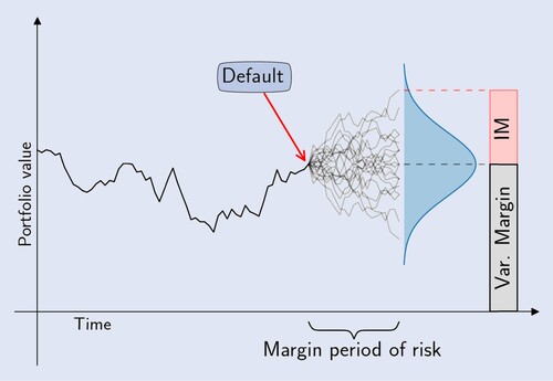
Figure 2. Standard initial margin model (SIMM).

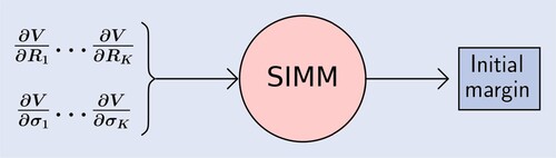
Figure 3. Definition margin value adjustment (MVA).

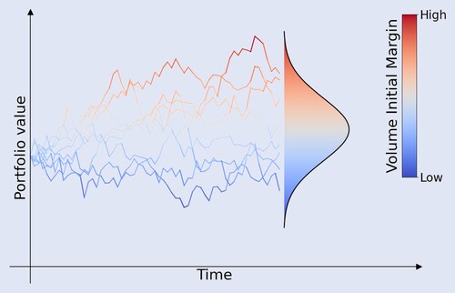
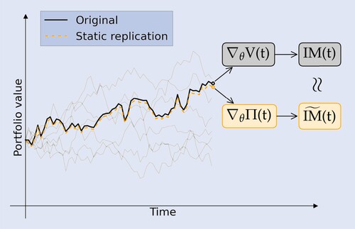
Figure 4. MVA through static replication.

Problem overview

1. Initial Margin (IM) is a form of collateral, which serves as a protection against the 99% value-at-risk of the exposure change during the margin period of risk (figure 1).

2. The industry standard approach to IM quantification is the Standard Initial Margin Model (SIMM), which takes the portfolio sensitivities as input (figure 2).

3. The expected funding cost of posting IM is called Margin Value Adjustment (MVA). Quantifying MVA requires the simulation of future IM (i.e. portfolio sensitivities), which is a computational challenge (figure 3).

4. We propose a method to statically replicate a callable derivative with a portfolio of vanilla options. This simplifies the computation of path-wise sensitivities and future IM (figure 4).

2.1. Model and assumptions

First, we fix a finite time-horizon $[0,\overline{T}]$, on which we consider a continuous-time financial market. We assume the market is frictionless and free of arbitrage. We let the probability space $(\mathrm{\Omega },\mathcal{F},\mathbb{P})$ represent all possible states of the economy and the filtration $\mathbb{F}=({\mathcal{F}}_t{)}_{t\in [0,\overline{T}]}$ all information generated by the economy up to time-t.

We consider the notion of a bank account or money market account. Investments in the money market are assumed to compound a continuous, risk-free interest $r_t$. We refer to $r_t$ as the short-rate. The time-t value of a unit of currency invested in the money market at time-zero is denoted as $M_t$, and we assume it satisfies the following dynamics $\begin{array}{r}\mathrm{d}{M}_t=r_t{M}_t\mathrm{d}t,M_0=1\end{array}$ We denote by $\mathbb{Q}$ the risk-neutral measure equivalent to $\mathbb{P}$, which is associated with $M_t$ as the numéraire. Attainable claims denominated by the numéraire are assumed to be martingales under $\mathbb{Q}$, which guarantees the absence of arbitrage (Harrison and Pliska 1981).

Throughout this paper we shall consider short-rate dynamics that are captured by an affine term-structure model, as introduced in Duffie and Kan (1996). That means that the short-rate can be written as $\begin{array}{r}{r}_t=g\left(x_t\right)\end{array}$ for some function $g:{\mathbb{R}}^d\to \mathbb{R}$. The vector $x_t:=\left\{x_1\right(t),\dots ,x_d(t\left)\right\}$ denotes a Markovian system of state-variables in ${\mathbb{R}}^d$. The state-variables are assumed to satisfy an SDE of the form (1) $\begin{array}{r}\mathrm{d}{x}_t=\mu (t,x_t)\mathrm{d}t+\eta \left(t\right)\mathrm{d}{W}_t\end{array}$(1) with $W_t:=\left\{W_1\right(t),\dots ,W_d(t\left)\right\}$ denoting a d-dimensional Brownian motion under $\mathbb{Q}$ and functions $\mu :[0,\overline{T}]\times {\mathbb{R}}^d\to {\mathbb{R}}^d$ and $\eta :[0,\overline{T}]\to {\mathbb{R}}^{d\times d}$. We let $g(\cdot )$ and $\mu (t,\cdot )$ be affine functions of $x_t$, satisfying the standard regularity conditions, such that $x_t$ admits a strong solution. Note that we restrict our scope to the Gaussian subclass of affine short-rate models. This is done to impose an intuitive relationship between model parameters and model-implied option volatilities (see section 3.5). This will facilitate the tractability of the computations; the estimation of Vega in particular. Generalizations to state-dependent diffusion coefficients should be possible but will involve the differentiation of Fourier transforms. This increases the complexity of the problem and falls outside the scope of this paper.

A zero-coupon bond is a contract that guarantees the holder one unit of currency at a pre-specified maturity date T. We will denote its time-t value as $P(t,T)$ for $t\le T$. An important result for affine term-structure models, is that zero-coupon bond prices are exponential affine in $x_t$. See for example Andersen and Piterbarg (2010) and Duffie and Kan (1996) for details. Next to zero-coupon bonds, we will often refer to a related quantity, known as the zero-rate. We define a zero-rate as $\begin{array}{r}R(t,T):=-\frac{\log P(t,T)}{\tau }\end{array}$ where τ denotes the year fraction between date t and T. For simplicity, we will assume that the collateral rate used for discounting and the instantaneous rate used to derive term-rates are both implied by the same short-rate $r_t$. In other words, our set-up will be a classic single-curve model environment. As term rates, we consider the classic, forward-looking LIBOR. Similarly one could consider a backward-looking, RFR-based term rate. In certain markets, the IBOR benchmark is discontinued, in favor of such set-in-arrears term rates (see Lyashenko and Mercurio 2019). As forward rates of forward- and backward-looking term rates are equivalent before the start of the accrual period, their treatment within this framework would mostly be the same.

2.2. Interest rate derivatives

The focus of this work will be on modeling Bermudan swaptions. Here we briefly introduce related derivatives and notation.

1. Interest rate swap: We consider fixed-for-floating interest rate swaps, where floating LIBOR payments are exchanged against fixed rate payments on dates $T_0,\dots ,T_M$. The year-fraction between $T_{j-1}$ and $T_j$ will be denoted ${\tau }_j$.

2. European swaption: A European swaption is a contract, which gives the holder the right, but not the obligation to enter an fixed-for-floating interest rate swap with pre-specified fixed rate K at a pre-specified future inception date $T_0$. Considering the annuity $A_{0,M}\left(t\right):=\sum _{m=1}^M{\tau }_{m}P(t,T_m)$ as numéraire, the risk-neutral value of a swaption (see Filipovic 2009) can be expressed as (2) $\begin{array}{r}{V}_t=A_{0,M}\left(t\right){\mathbb{E}}^{0,M}\left[{\left(\delta \left(S_{0,M}\right(T_0)-K)\phantom{|}\right)}^{+}|{\mathcal{F}}_t\right]\end{array}$(2) where the expectation above is taken under the annuity measure ${\mathbb{Q}}^{0,M}$. The parameter δ distinguishes between a payer ($\delta =1$) and a receiver ($\delta =-1$) swaption. Under the assumption that the swap rate has Gaussian dynamics, the swaption price can evaluated using Bachelier's formula (see Musiela and Rutkowski 1997). Given a swaption has market price $V_{\mathrm{mkt}}(t,K)$, the implied normal volatility is defined as the unique scalar ${\sigma }_{\mathrm{imp}}$ that solves the equation $\begin{array}{r}{V}_{\mathrm{Bach}}(t,{\sigma }_{\mathrm{imp}},K)=V_{\mathrm{mkt}}(t,K)\end{array}$

3. Bermudan swaption: A Bermudan swaption is a contract, which gives the holder the right to enter a fixed-for-floating interest rate swap with maturity $T_M$ at any of the dates $T_0,\dots ,T_{M-1}$ at a pre-specified fixed rate K. Should the holder of the Bermudan choose to exercise at $T_m$, the payoff is given by $\begin{array}{rl}h(T_m,x_{T_m})& :=h_m\left(x_{T_m}\right)\\ & =\delta A_{m,M}(T_m;x_{T_m})\left[S_{m,M}\right(T_m;x_{T_m})-K]\end{array}$ The value of a Bermudan swaption can be represented through a dynamic programming formulation, in which the price is captured by means of a backward recursion (Glasserman 2004), given by $\begin{array}{rl}& V(t;x_t)\\ & =\{\begin{array}{ll}max\left\{h_{M-1}\right(x_t),0\}& \mathrm{if}t=T_{M-1}\\ max\left\{h_m\right(x_t),C_m(t,x_t\left)\right\}& \mathrm{if}t=T_m,\\ & m=0,\dots ,M-2\\ C_{m-1}(t,x_t)& \mathrm{if}t\in (T_{m-1},T_m)\end{array}\end{array}$ where $C_m$ represents the continuation value of the contract.

2.3. Credit risk metrics

In this work, we will consider credit exposure and forward sensitivity profiles of Bermudan swaptions. Exposure is essential for CVA computation. Product sensitivities, Delta and Vega in particular, serve as an input to ISDA SIMM calculations for initial margin.

2.3.1. Exposure and CVA

The expected positive exposure (EPE) of a financial contract with price $V_t$ at time $t\ge 0$ is $\begin{array}{r}\mathrm{EPE}\left(t\right):={\mathbb{E}}^{\mathbb{Q}}[e^{-{\int }_0^t{r}_u\mathrm{d}u}max\{V_t,0\}|{\mathcal{F}}_0]\end{array}$ Expected positive exposure represents the expected loss on a claim in the event of a counterparty defaulting at a given time $t\ge 0$ (Gregory 2020). The expectation is evaluated under the risk-neutral measure $\mathbb{Q}$. Exposure is a key ingredient in the quantification of counterparty risk at trade or counterparty level through CVA. CVA is the difference between the total value of a derivative in a market that is completed with counterparty risk and its default-free value (Burgard and Kjaer 2013). Let $\tau \ge 0$ denote the default time of the counterparty. Assuming τ is independent of exposure (i.e. ignoring wrong- or right-way risk), CVA can be computed as follows Green (2015) (3) $\begin{array}{rl}\mathrm{CVA}& =(1-\mathrm{RR}){\int }_0^T\mathrm{EPE}\left(u\right)\mathrm{d}\mathbb{Q}(\tau =u)\\ & \approx \mathrm{LGD}\sum _{i=1}^n\mathrm{EPE}\left(t_i\right)\times \mathrm{PD}(t_{i-1},t_i)\end{array}$(3) with RR denoting the recovery rate, LGD the loss given default and PD the probability of default of the counterparty. A common approach in the literature is to model the default time τ as an ${\mathcal{F}}_t-$adapted stopping time using a Cox-construction (Jeanblanc and Li 2020). In that case, the survival function of the counterparty follows an exponential distribution, i.e. $\mathbb{Q}(\tau >t)=\exp \{-\mathrm{\Lambda }(t\left)\right\}$ with $\mathrm{\Lambda }\left(t\right)$ denoting a hazard function. The hazard function can be specified in terms of a hazard rate $\lambda \left(t\right)$, which yields $\mathrm{\Lambda }\left(t\right)={\int }_0^t\lambda \left(u\right)\mathrm{d}u$. Therefore, the probability of default can be written as (4) $\begin{array}{r}\mathrm{PD}(t_{i-1},t_i)=e^{-{\int }_0^{t_{i-1}}\lambda \left(u\right)\mathrm{d}u}-e^{-{\int }_0^{t_i}\lambda \left(u\right)\mathrm{d}u}\end{array}$(4)

2.3.2. Initial margin and MVA

An important means to reduce the exposure at risk is the exchange of collateral. In this work, we will consider initial margin (IM) and its related funding costs. IM is a protection against exposure changes during the margin period of risk, the time interval after a default when outstanding positions are not yet settled, but VM is no longer updated (Green and Kenyon 2015). Typically, IM reflects the 99% value-at-risk of the portfolio change over a 10-day time interval. Throughout this work, we will consider the Standard Initial Margin Model (SIMM) to be the default method for IM computations. The main take-away from SIMM–IM is that it is a sensitivity-based approach. The idea is that the response of an instrument to a risk-factor shock is efficiently approximated by multiplying the instrument's risk-factor sensitivity by the corresponding shock size (International Swaps and Derivatives Association, Inc 2016). We will provide a brief summary of SIMM below, but refer to International Swaps and Derivatives Association, Inc (2020) for details.

Consider risk-factors $\mathit{\theta }:=({\theta }_1,\dots ,{\theta }_K{)}^{\mathrm{\top }}$ and denote the 10-day risk-factor increments as $\mathrm{\Delta }{\theta }_1,\dots ,\mathrm{\Delta }{\theta }_K$. The variance of the total response of an instrument $V_t$ to each shock $\mathrm{\Delta }{\theta }_i$ is computed as $\begin{array}{r}\mathbb{V}\mathrm{ar}\left(\sum _{i=1}^K\frac{\mathrm{\partial }{V}_t}{\mathrm{\partial }{\theta }_i}\mathrm{\Delta }{\theta }_i\right)={\left[D_{\theta }{V}_t\right]}^{\mathrm{\top }}{\mathrm{\Sigma }}_{\theta }\left[D_{\theta }{V}_t\right]\end{array}$ where $D_{\theta }{V}_t$ denotes the gradient of $V_t$ w.r.t. $\mathit{\theta }$ and ${\mathrm{\Sigma }}_{\theta }$ denotes the covariance matrix of $\mathit{\theta }$. If the total response defined above, is assumed to be approximately Gaussian with mean zero, the VaR can be estimated as follows $\begin{array}{r}{\mathrm{VaR}}_{0.99}\left(\mathrm{\Delta }{V}_t\right)\approx {\mathrm{\Phi }}^{-1}\left(0.99\right)\sqrt{{\left[D_{\theta }{V}_t\right]}^{\mathrm{\top }}{\mathrm{\Sigma }}_{\theta }\left[D_{\theta }{V}_t\right]}\end{array}$ Where ${\mathrm{\Phi }}^{-1}$ denotes the inverse of the standard normal CDF. For interest rate derivatives, ISDA distinguishes three relevant types of risk-factors, namely Delta-risk, Vega-risk and Curvature-risk, the latter referring to the second-order Gamma impact. The total IM is given by (5) $\begin{array}{r}\mathrm{IM}:={\mathrm{Margin}}_{\mathrm{Delta}}+{\mathrm{Margin}}_{\mathrm{Vega}}+{\mathrm{Margin}}_{\mathrm{Curvature}}\end{array}$(5) where each component represents a VaR estimation w.r.t. a type of underlying risk-factors, i.e. market interest rates and market implied volatilities. The risk-factors of each type are subdivided into twelve buckets, corresponding to the yields at the tenors $\mathcal{T}:=\{2W,1M,3M,6M,1Y,2Y,3Y,5Y,10Y,15Y,20Y,30Y\}$. Hence for each component one needs to compute the corresponding 12-dimensional sensitivity vector, which are specified as (see also International Swaps and Derivatives Association, Inc 2020):

Delta	: The PV01 of the instrument $V_t$ w.r.t. the risk-free interest rate $R_k$ at tenor ${\tau }_k\in \mathcal{T}$, i.e. ${\mathrm{\Delta }}_k=V_t(R_k+1\mathrm{bp})-V_t\left(R_k\right)$.
Vega	: The sensitivity of the instrument $V_t$ w.r.t. volatility risk-factor ${\sigma }_k$, i.e. ${\mathcal{V}}_k=V_t({\sigma }_k+1\mathrm{\%})-V_t\left({\sigma }_k\right)$. Here, ${\sigma }_k$ denotes the the implied at-the-money volatility of a swaption with an expiry time equal to ${\tau }_k\in \mathcal{T}$.
Curvature	: Curvature margin represents the second-order impact of the interest rate risk-factors to the VaR estimate. In SIMM, the Gamma is approximated with a Vega-Gamma relationship. Therefore, the computation of Curvature margin takes the Vega sensitivity vector as input, similar to Vega margin.

For SIMM–IM quantification in practice, the user only needs to compute the portfolio sensitivities. The other parameters are provided by ISDA in an annual publication.

A key difference between VM and IM is that the former is symmetric. VM reflects the value of the underlying trade and can be rehypothecated. This means the receiver can reuse the collateral, for example in the margin agreement of an opposite transaction. In contrast, IM reflects the risk of a trade and must be exchanged in both directions, without netting the amounts. The collateral is often required to be posted on a segregated account and therefore cannot be rehypothecated (Gregory 2020). As a result, IM must be funded by the dealer, which comes at a cost. The expected lifetime cost of posting IM against a portfolio is called Margin Value Adjustment (MVA) (Green and Kenyon 2015).

The size of MVA is driven by the dynamic IM profile of the portfolio and the funding spread that applies to the IM posting. As the volume of IM is dependent on the state of the economy, $\left\{\mathrm{IM}\right(t):t\in [0,T\left]\right\}$ represents a stochastic process. The expected initial margin (EIM) of a financial contract at time $t\ge 0$ is defined as $\begin{array}{r}\mathrm{EIM}\left(t\right):={\mathbb{E}}^{\mathbb{Q}}\left[e^{-{\int }_0^t{r}_u\mathrm{d}u}\mathrm{IM}\right(t\left)|{\mathcal{F}}_0\right]\end{array}$ EIM represents the expected volume of IM that needs to be posted by the dealer at a given time $t\ge 0$ (Gregory 2020). With this expression at hand, MVA can be computed as follows (6) $\begin{array}{rl}\mathrm{MVA}& ={\int }_0^T\mathrm{FS}\left(u\right)\mathrm{EIM}\left(u\right)\mathrm{d}u\\ & \approx \sum _{i=1}^n\mathrm{FS}\left(t_i\right)\times \mathrm{EIM}\left(t_i\right)\times (t_i-t_{i-1})\end{array}$(6) with FS denoting the funding spread, which reflects the spread on the collateral rate w.r.t. the risk-free rate (Green and Kenyon 2015).

3. The static replication method

In this section, we describe the algorithm that is used to compose a static replication portfolio for a Bermudan swaption. The algorithm is embedded in a Monte Carlo framework and relies on a regress-later technique. See Glasserman and Yu (2004) for a general introduction to regress-later. The method is strongly inspired by the work of Jain and Oosterlee (2015) and extends the approach that is presented in Lokeshwar et al. (2022) and Hoencamp et al. (2023).

In Jain and Oosterlee (2015), it is shown that early-exercise options can be priced with an application of a regress-later technique. As such, the ‘later’ option price $V_{T_{m+1}}$ is regressed against the ‘later’ risk-factor realization $x_{T_{m+1}}$. The continuation value is subsequently estimated by evaluating the conditional expectation of the regressed option value, i.e. $\begin{array}{rl}{C}_m\left(T_m\right)& =M_{T_m}{\mathbb{E}}^{\mathbb{Q}}\left[\frac{V_{T_{m+1}}}{M_{T_{m+1}}}|{\mathcal{F}}_{T_m}\right]\\ & \approx M_{T_m}{\mathbb{E}}^{\mathbb{Q}}\left[\frac{\sum _{k=1}^K{\alpha }_k{\varphi }_k\left(x_{T_{m+1}}\right)}{M_{T_{m+1}}}|{\mathcal{F}}_{T_m}\right]\end{array}$ which can be computed in (semi) closed-form for an appropriate choice of basis-functions ${\varphi }_k$.

In Lokeshwar et al. (2022), it is proposed to perform the regression with a shallow neural network (i.e. a feed-forward neural network with a single hidden layer). By considering the appropriate network structure, it is shown that the regression can be interpreted as a portfolio of short-maturity options. As a consequence, the continuation value can be evaluated by simply pricing the replication instruments. In Hoencamp et al. (2023), this approach is extended to an interest rate modeling framework. There it is shown that a Bermudan swaption can be semi-statically replicated by an options portfolio written on zero-coupon bonds. The central concept of the latter two studies is that if a portfolio perfectly reproduces the value function of a derivative security at some future time $T_j$ for every realization of the state-variables, the no-arbitrage condition implies that this portfolio will also replicate the security at any time $t<T_j$, as long as no cash-flows can occur between t and $T_j$. Where a dynamic replicating portfolio needs to be rebalanced continuously through time, the semi-static replication only needs rebalancing on a finite number of instances.

The algorithm that is proposed in this paper builds further on the foundations that were laid by Jain and Oosterlee (2015), Lokeshwar et al. (2022) and Hoencamp et al. (2023). We suggest two main novelties compared to the earlier studies

• We propose to use the swap rate as the regression variable, which is an implicit risk-factor in our model set-up. As a consequence, the regression can be interpreted as the payoff of a portfolio of European swaptions. We further elaborate on this in Section 3.4.

• We propose a new variation to the algorithm, which allows us to compose a replication that is not semi-static, but in fact truly static. In other words, this algorithm lets one compose a portfolio at time zero, which will mirror the value of the Bermudan until it is either exercised or expired, without the need of updating the portfolio at intermediate time-points. We further elaborate on this in Section 3.3.

3.1. The algorithm

The algorithm is executed in an iterative manner, moving backwards in time. Starting at the final exercise date $T_{M-1}$, a regression is performed to determine the weights and strikes of an options portfolio which replicates the Bermudan's payoff. This replication is subsequently used to estimate the value of the Bermudan at the preceding monitor date, yielding the target function of the consecutive regression. This process is repeated until the first monitor date $T_0$ and a portfolio has been composed which statically replicates the Bermudan between time-zero and its final exercise date. Below we will describe the algorithm in more detail.

Start by sampling N trajectories of the underlying state-variable. For each realization of $x_{T_{M-1}}$, compute the Bermudan swaption payoff at $T_{M-1}$ (the final exercise opportunity) $f_{M-1}\left(x_{T_{M-1}}\right)=max\left\{h_{M-1}\right(x_{T_{M-1}}),0\}$. This will act as the target function of the first regression. Now recursively execute the following steps for $m=M-1,\dots ,0$:

1. Select and sample the regression variable

Select an asset $z_m\left(t\right)=\left\{z_{m,1}\right(t,x_t),\dots ,z_{m,d}(t,x_t\left)\right\}$ taking value in ${\mathbb{R}}^d$ that will act as the independent regression variable. For compactness, we will suppress the dependency of $z_m$ on the state variable $x_t$, when clear from the context. The asset(s) should satisfy the following conditions:

• $z_m\left(T_m\right)$ is a square integrable random variable on the probability space $(\mathrm{\Omega },{\mathcal{F}}_{T_m},\mathbb{Q})$.

• For each $m=0,\dots ,M-1$, the realization $f_m\left(x_{T_m}\right)$ is uniquely determined by $z_m\left(T_m\right)$.

• The parametrization $\left\{\right(z_m(T_m;x),f_m\left(x\right)\phantom{|}):x\in {\mathbb{R}}^d\}$ is continuous.

where $f_m$ denotes a target function, which we define in (8(8) $\begin{array}{r}{f}_m\left(x\right)=\{\begin{array}{l}{q}_m\left(x\right)\cdot max\{h_m\left(x\right),0\}\\ \mathrm{if}m=M-1\\ q_m\left(x\right)\cdot max\{h_m\left(x\right)-{\tilde{C}}_m(T_m,x),0\}\\ \mathrm{if}m=M-2,\dots ,0\end{array}\end{array}$(8) ) below. Subsequently compute for each sample path the realizations of $z_m\left(T_m\right)$.

2. Regress the target function

Consider a regression function $G_m:{\mathbb{R}}^d\to \mathbb{R}$ that is defined as (7) $\begin{array}{r}{G}_m={\psi }_2\circ A_2\circ {\psi }_1\circ A_1\end{array}$(7) Here we denote by $A_1:{\mathbb{R}}^d\to {\mathbb{R}}^n$, $A_2:{\mathbb{R}}^n\to \mathbb{R}$ affine functions of the form $\begin{array}{r}{A}_1\left(y\right)\mapsto {\mathit{w}}_{\mathbf{1}}y+{\mathit{b}}_{\mathbf{1}}\mathrm{and}{A}_2\left(y\right)\mapsto {\mathit{w}}_{\mathbf{2}}y+b_2\end{array}$ with ${\mathit{w}}_{\mathbf{1}}\in {\mathbb{R}}^{d\times n}$, ${\mathit{w}}_{\mathbf{2}}\in {\mathbb{R}}^{n\times 1}$, ${\mathit{b}}_{\mathbf{1}}\in {\mathbb{R}}^n$ and $b_2\in \mathbb{R}$. Furthermore we denote by ${\psi }_1:{\mathbb{R}}^n\to {\mathbb{R}}^n$, ${\psi }_2:\mathbb{R}\to \mathbb{R}$ activation functions of the form $\begin{array}{r}{\psi }_1\left(y\right)\mapsto (max\{y_1,0\},\dots ,max\{y_n,0\})\mathrm{and}{\psi }_2\left(y\right)\mapsto y\end{array}$ Additionally, consider a target function $f_m:{\mathbb{R}}^d\to \mathbb{R}$ of the form (8) $\begin{array}{r}{f}_m\left(x\right)=\{\begin{array}{l}{q}_m\left(x\right)\cdot max\{h_m\left(x\right),0\}\\ \mathrm{if}m=M-1\\ q_m\left(x\right)\cdot max\{h_m\left(x\right)-{\tilde{C}}_m(T_m,x),0\}\\ \mathrm{if}m=M-2,\dots ,0\end{array}\end{array}$(8) where $q_m\left(x\right)$ denotes a possible scaling factor. The rationale behind this target function is that we aim to regress the fraction of the option value that is lost, when an exercise date passes, but the option is not exercised. We provide an elaborate motivation and interpretation in section 3.3.

Subsequently, optimize the parameters ${\text{β}}_m=\{{\mathit{w}}_{\mathbf{1}},{\mathit{w}}_{\mathbf{2}},{\mathit{b}}_{\mathbf{1}},b_2\}$, such that $G_m\left(z_m\right(T_m);{\text{β}}_m)$ fits the target function $f_m\left(x_{T_m}\right)$. The parameters are determined by minimizing the cost function (9) $\begin{array}{rl}{L}_m\left(\text{β}\right)& ={\mathbb{E}}^{\mathbb{Q}}\left[{(G_m(z_m\left(T_m\right);\text{β}\phantom{|})-f_m\left(\phantom{|}{x}_{T_m}\right)\phantom{|})}^2\right]\end{array}$(9) (10) $\begin{array}{rl}& \approx \frac{1}{N}\sum _{n=1}^N{(G_m\left(z_m\right(n);\text{β}\phantom{|})-f_m\left(\phantom{|}{x}_{T_m}\right(n\left)\right)\phantom{|})}^2\end{array}$(10) where $z_m\left(n\right)$ and $x_{T_m}\left(n\right)$ denote sampled realizations of the asset and the state variable, respectively, on a corresponding MC path.

3. Estimate the continuation value

Finally, the continuation value of the Bermudan swaption at the preceding exercise date $T_{m-1}$ is estimated by calculating (11) $\begin{array}{r}{\tilde{C}}_{m-1}(T_{m-1},x_{T_{m-1}})=\sum _{j=m}^{M-1}{M}_{T_{m-1}}{\mathbb{E}}^{\mathbb{Q}}\left[\frac{G_j(z_j\left(T_j\right);{\text{β}}_j)}{M_{T_j}\cdot q_j\left(x_{T_j}\right)}|x_{T_{m-1}}\right]\end{array}$(11) With an appropriate choice of $z_m$, this can be computed in closed-form or approximated with an efficient numerical routine.

3.2. Interpretation of the regression function

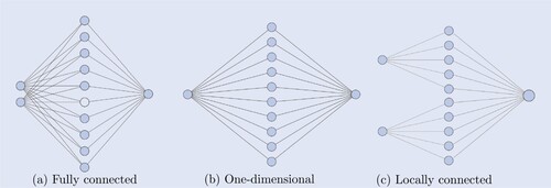
The regression function as presented in (7(7) $\begin{array}{r}{G}_m={\psi }_2\circ A_2\circ {\psi }_1\circ A_1\end{array}$(7) ) can be considered a shallow neural network, i.e. a feed-forward neural network with a single hidden layer. The structure is graphically represented in figure 5(a). The outcome of the first hidden layer is a vector in ${\mathbb{R}}^n$, consisting of n neurons. Each individual neuron $O_{m,i}$ is calculated as $\begin{array}{r}{O}_{m,i}=max\{\sum _{j=1}^d{w}_{\mathrm{ij}}{z}_{m,i}\left(T_m\right)+b_i,0\}\end{array}$ The functional form of each hidden node thus corresponds to the payoff of an arithmetic basket option written on $z_{m,1},\dots ,z_{m,d}$.

Figure 5. Neural network structures. (a) Fully connected. (b) One-dimensional and (c) Locally connected.

The outcome of the second layer is calculated as $\begin{array}{r}\sum _{i=1}^n{w}_i{O}_{m,i}+b\end{array}$ The functional form of the outcome of the neural network, hence corresponds to the payoff of a weighted portfolio of basket options, plus a zero-coupon bond maturing at $T_m$. Computing the conditional expectation given in (11(11) $\begin{array}{r}{\tilde{C}}_{m-1}(T_{m-1},x_{T_{m-1}})=\sum _{j=m}^{M-1}{M}_{T_{m-1}}{\mathbb{E}}^{\mathbb{Q}}\left[\frac{G_j(z_j\left(T_j\right);{\text{β}}_j)}{M_{T_j}\cdot q_j\left(x_{T_j}\right)}|x_{T_{m-1}}\right]\end{array}$(11) ) can be interpreted as evaluating the risk-neutral price of this portfolio.

3.3. A static replication

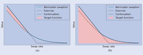
Let ${\mathrm{\Pi }}_m\left(t\right)$ denote an options portfolio maturing at $T_m$ with payoff equal to (12) $\begin{array}{r}{\mathrm{\Pi }}_m\left(T_m\right)=\frac{1}{q_m\left(x_{T_m}\right)}{G}_m(z_m\left(T_m\right);{\text{β}}_m)\end{array}$(12) By the deliberate choice of the target function $f_m$ in (8(8) $\begin{array}{r}{f}_m\left(x\right)=\{\begin{array}{l}{q}_m\left(x\right)\cdot max\{h_m\left(x\right),0\}\\ \mathrm{if}m=M-1\\ q_m\left(x\right)\cdot max\{h_m\left(x\right)-{\tilde{C}}_m(T_m,x),0\}\\ \mathrm{if}m=M-2,\dots ,0\end{array}\end{array}$(8) ), the payoff of this portfolio yields the approximation $\begin{array}{rl}{\mathrm{\Pi }}_m\left(T_m\right)& \approx max\{h_m\left(x_{T_m}\right)-{\tilde{C}}_m(T_m,x_{T_m}),0\}\\ & =max\{h_m\left(x_{T_m}\right),{\tilde{C}}_m(T_m,x_{T_m})\}-{\tilde{C}}_m(T_m,x_{T_m})\end{array}$ which is graphically represented by the red area in figure 6(a). As a consequence of the no-arbitrage condition, it follows that at any time $t<T_m$ the risk-neutral portfolio value yields the approximation ${\mathrm{\Pi }}_m\left(t\right)\approx C_{m-1}(t,x_t)-C_m(t,x_t)$. By a repeated argument, whenever $t\in (T_{m-1},T_m)$ we have $\begin{array}{r}\sum _{i=m}^{M-1}{\mathrm{\Pi }}_i\left(t\right)\approx C_{m-1}(t,x_t)=V\left(t\right)\end{array}$ The combined portfolio $\mathrm{\Pi }\left(t\right):=\sum _{i=0}^{M-1}{\mathrm{\Pi }}_i\left(t\right)$, composed at t = 0, can be interpreted as a fully static replication of the Bermudan swaption. Whenever a monitor date $T_m$ is reached, subportfolio ${\mathrm{\Pi }}_m$ expires. Then, two things could happen:

• $\mathit{C}\mathbf{(}{\mathit{T}}_{\mathit{m}}\mathbf{,}{\mathit{x}}_{{\mathit{T}}_{\mathit{m}}}\mathbf{)}\mathbf{\le }{\mathit{h}}_{\mathit{m}}\mathbf{\left(}{\mathit{x}}_{{\mathit{T}}_{\mathit{m}}}\mathbf{\right)}:$ The holder exercises the Bermudan and the value of $\sum _{i=m+1}^{M-1}{\mathrm{\Pi }}_i$ plus the payoff of ${\mathrm{\Pi }}_m$ will equal the exercise value.

• $\mathit{C}\mathbf{(}{\mathit{T}}_{\mathit{m}}\mathbf{,}{\mathit{x}}_{{\mathit{T}}_{\mathit{m}}}\mathbf{)}\mathbf{>}{\mathit{h}}_{\mathit{m}}\mathbf{\left(}{\mathit{x}}_{{\mathit{T}}_{\mathit{m}}}\mathbf{\right)}:$ The holder holds the Bermudan, subportfolio ${\mathrm{\Pi }}_m$ expires worthless and $\sum _{i=m+1}^{M-1}{\mathrm{\Pi }}_i$ will continue to replicate the Bermudan.

Figure 6. Target functions regress-later: two approaches. (a) Fully static replication and (b) Semi-static replication.

Thus, portfolio Π will mirror the Bermudan swaption value until it is either matured or exercised.

The algorithm presented in this work is a variation to the semi-static replication approach presented in Lokeshwar et al. (2022) and Hoencamp et al. (2023). There, the target function $f_m$ is selected such that the portfolio payoff ${\mathrm{\Pi }}_m$ yields the approximation $\begin{array}{r}{\mathrm{\Pi }}_m\left(T_m\right)\approx max\{h_m\left(x_{T_m}\right),{\tilde{C}}_m(T_m,x_{T_m})\}\end{array}$ which is graphically represented by the red area in figure 6(b). In that case, subportfolio ${\mathrm{\Pi }}_m$ is set-up on $T_{m-1}$, it replicates the Bermudan on the time-interval $(T_{m-1},T_m)$ and expires at $T_m$. Its payoff will equal the exercise value of the Bermudan, or suffice to set-up subportfolio ${\mathrm{\Pi }}_{m+1}$ in case the Bermudan is continued. The advantage of the latter approach is that only ${\mathrm{\Pi }}_m\left(t\right)$ needs to be priced in order to value the Bermudan, rather than $\sum _{i=m}^{M-1}{\mathrm{\Pi }}_i\left(t\right)$. A disadvantage is that the replication is only semi-static and needs rebalancing on each monitor date $T_m$.

3.4. Estimation of the continuation value

How the continuation value as given in (11(11) $\begin{array}{r}{\tilde{C}}_{m-1}(T_{m-1},x_{T_{m-1}})=\sum _{j=m}^{M-1}{M}_{T_{m-1}}{\mathbb{E}}^{\mathbb{Q}}\left[\frac{G_j(z_j\left(T_j\right);{\text{β}}_j)}{M_{T_j}\cdot q_j\left(x_{T_j}\right)}|x_{T_{m-1}}\right]\end{array}$(11) ) is computed, depends on the specification of the model and the selection of the regression asset. In the general case, the portfolio ${\mathrm{\Pi }}_m$ can be interpreted as a portfolio of arithmetic basket options. The valuation of a basket option is typically still not an easy exercise. However, with the appropriate constraints on the neural network structure used for the regression, the replicating portfolio can be reduced to a set of European options. A first approach would be to consider a one-dimensional regression asset, which corresponds to the design depicted in figure 5(b). This would be appropriate under a one-factor model. A second approach would be to constrain matrix $A_1$ to have only one non-zero entry in each row. This corresponds to the neural network design depicted in figure 5(c). In the numerical examples included in this work, we will be considering a 1-factor model environment. Generalizations to multi-factor models have been described in Hoencamp et al. (2023). We will consider the following assumptions:

• Regression asset: select $z_m\left(t\right)=S_{m,M}\left(t\right)$.

• Scaling factor: set $q_m\left(x_t\right)=\frac{1}{A_{m,M}(t,x_t)}$.

Under the assumptions stated above, the (sub)portfolio ${\mathrm{\Pi }}_m$ as defined in (12(12) $\begin{array}{r}{\mathrm{\Pi }}_m\left(T_m\right)=\frac{1}{q_m\left(x_{T_m}\right)}{G}_m(z_m\left(T_m\right);{\text{β}}_m)\end{array}$(12) ), can be interpreted as a portfolio of European swaptions, written on the swap rate $S_{m,M}\left(t\right)$.¹ The valuation of ${\mathrm{\Pi }}_m\left(t\right)$ for some $t<T_m$ comes down to $\begin{array}{rl}& {\mathrm{\Pi }}_m\left(t\right)\\ & =M_t{\mathbb{E}}^{\mathbb{Q}}\left[\frac{G_m(z_m\left(T_m\right);{\text{β}}_j)}{M_{T_m}\cdot q_m\left(x_{T_m}\right)}|x_t\right]\\ & =M_t{\mathbb{E}}^{\mathbb{Q}}\left[A_{m,M}\right(T_m\left)\frac{\sum _{i=1}^n{w}_{2,i}max\{w_{1,i}{S}_{m,M}\left(T_m\right)+b_i,0\}}{M_{T_j}}|x_t\right]\\ & =\sum _{i=1}^n{w}_{2,i}{A}_{m,M}\left(t\right){\mathbb{E}}^{m,M}[max\{w_{1,i}{S}_{m,M}\left(T_m\right)+b_i,0\}|x_t]\end{array}$ where the expectation in the last line is taken under the annuity measure ${\mathbb{Q}}^{m,M}$ associated to the numéraire $A_{m,M}\left(t\right)$. The expression above should be recognized as a linear combination of European swaption prices (see equation (2(2) $\begin{array}{r}{V}_t=A_{0,M}\left(t\right){\mathbb{E}}^{0,M}\left[{\left(\delta \left(S_{0,M}\right(T_0)-K)\phantom{|}\right)}^{+}|{\mathcal{F}}_t\right]\end{array}$(2) )). The parameter $w_{1,i}$ distinguishes between a payer ($w_{1,i}>0$) and receiver ($w_{1,i}<0$) swaption. The parameter $w_{2,i}$ distinguishes between a long ($w_{2,i}>0$) and a short ($w_{2,i}<0$) position in the swaption contract.

3.5. Valuation of the replicating portfolio

Under the assumptions of section 3.4, portfolio ${\mathrm{\Pi }}_m$ consists of European swaptions, which means the valuation comes down to pricing each individual option. We apply a coefficient freezing technique, described in Andersen and Piterbarg (2010) and Schrager and Pelsser (2006). With this technique, the swap rate process is approximated as a generalized arithmetic Brownian motion, by freezing the stochastic terms in its diffusion. The option's implied volatility can then be approximated by integrating the ‘frozen’ diffusion coefficient. We briefly summarize the method below, and refer to Andersen and Piterbarg (2010) and Schrager and Pelsser (2006) for details.

Consider the dynamics of the swap rate. By Itô's lemma, it can be established that $S_{m,M}$ satisfies the SDE $\begin{array}{r}\mathrm{d}{S}_{m,M}\left(t\right)=(\dots )\mathrm{d}t+{\left[D_x{S}_{m,M}\right(t\left)\right]}^{\mathrm{\top }}\eta \left(t\right)\cdot \mathrm{d}{W}_t\end{array}$ Considering the annuity as numéraire, the swap rate can regarded as the quotient of some tradable assets and the numéraire itself. As a consequence, the swap rate is a Martingale under the annuity measure ${\mathbb{Q}}^{m,M}$ (Jamshidian 1997). Hence, for $0\le t\le T\le T_m$ we can write (13) $\begin{array}{r}{S}_{m,M}\left(T\right)=S_{m,M}\left(t\right)+{\int }_t^T{\mathrm{\Sigma }}_{m,M}\left(u{)}^{\mathrm{\top }}\eta \right(u)\cdot \mathrm{d}{W}_u^{m,M}\end{array}$(13) where $W^{m,M}$ denotes a d-dimensional ${\mathbb{Q}}^{m,M}$ Brownian motion and ${\mathrm{\Sigma }}_{m,M}\left(t\right):=\left[D_x{S}_{m,M}\right(t){]}^{\mathrm{\top }}$. Working out the diffusion for $i=1,\dots ,d$ yields (14) $\begin{array}{rl}{\mathrm{\Sigma }}_{m,M}\left(t\right)& =B(t,T_M)\frac{P(t,T_M)}{A_{m,M}\left(t\right)}-B(t,T_m)\frac{P(t,T_m)}{A_{m,M}\left(t\right)}\\ & -S_{m,M}\left(t\right)\sum _{l=m+1}^M{\tau }_{l}B(t,T_l)\frac{P(t,T_l)}{A_{m,M}\left(t\right)}\end{array}$(14) The diffusion coefficient is stochastic, due to the $\frac{P(t,T_i)}{A_{m,M}\left(t\right)}$ terms. However, these terms again represent the quotient of a tradable asset and the numéraire. It is conjectured in Schrager and Pelsser (2006), that these terms are Martingales with low quadratic variation. A good approximation is therefore achieved by freezing them at their time-t value, resulting in a deterministic diffusion coefficient ${\tilde{\mathrm{\Sigma }}}_{m,M}\left(u\right)$ for $u\in [t,T]$. It follows (15) $\begin{array}{r}{S}_{m,M}\left(T\right)\approx {\tilde{S}}_{m,M}\left(T\right):=S_{m,M}\left(t\right)+{\int }_t^T{\tilde{\mathrm{\Sigma }}}_{m,M}\left(u{)}^{\mathrm{\top }}\eta \right(u)\cdot d{W}_u^{m,M}\end{array}$(15) The approximation ${\tilde{S}}_{m,M}\left(T\right)$ conditioned on ${\mathcal{F}}_t$ is normally distributed. Applying Itô isometry allows us to approximate the implied volatility of an option written on $S_{m,M}$, which yields (16) $\begin{array}{rl}& {\tilde{\sigma }}_{\mathrm{imp}}(t,T)\\ & =\sqrt{\frac{1}{T-t}{\mathbb{E}}^{m,M}\left[{\Vert {\int }_t^T{\tilde{\mathrm{\Sigma }}}_{m,M}\left(u{)}^{\mathrm{\top }}\eta \right(u)\cdot \mathrm{d}{W}_u^{m,M}\Vert }_2^2|x_t\right]}\end{array}$(16) (17) $\begin{array}{rl}& =\sqrt{\frac{1}{T-t}{\int }_t^T\Vert {\tilde{\mathrm{\Sigma }}}_{m,M}\left(u{)}^{\mathrm{\top }}\eta \right(u){\Vert }_2^2\mathrm{d}u}\end{array}$(17) Substituting ${\tilde{\sigma }}_{\mathrm{imp}}(t,T)$ into Bachelier's formula results is the desired swaption price.

4. Numerical algorithms and mathematical consistency

In this section, we describe the numerical routines for computing sensitivities along the Monte Carlo path. In short, we show how to compute the sensitivities of the replicating portfolio in a time-consistent manner. This involves the differentiation of the replicating instrument values (i.e. greeking) and the differentiation of the portfolio weights.

Our approach to the latter is inspired by the work of Jain et al. (2019). In Jain et al. (2019) a regress-later approach is considered, which utilizes ordinary least-square regression. As such, the weights of the basis-functions can be obtained explicitly as a function of the risk-factor and consistently differentiated. In this paper, only an implicit relation between the risk-factors and the portfolio weights is known through the minimized cost function (equation (10(10) $\begin{array}{rl}& \approx \frac{1}{N}\sum _{n=1}^N{(G_m\left(z_m\right(n);\text{β}\phantom{|})-f_m\left(\phantom{|}{x}_{T_m}\right(n\left)\right)\phantom{|})}^2\end{array}$(10) )). Yet, we show that an estimator of the weight sensitivities can still be obtained through an application of the implicit function theorem.

An advantage of our approach is that it should be easier to evaluate sensitivities to implicit risk-factors, which are not directly modeled. In the context of MVA this concerns the sensitivities to the realizations of future market rates and future implied volatilities. With regard to static replication, the replicating portfolio is selected such that the required future Delta and Vega are tractable to compute. In contrast, with, for example, an application of AD on LSM, this may not be straight-forward. It would require the computation pseudo Jacobian-inverses or adding plenty pseudo-interpolation-nodes to the term-structure of zero-rates and instantaneous volatilities, which may be a tedious task.

4.1. Notation and assumtions

Let $t\in [0,\overline{T})$ and let $V_t$ denote the time-t risk-neutral value of a Bermudan swaption with strike K and tenor structure $T_0,T_1,\dots T_M$, conditioned on the event that the option is not yet exercised at t. Next to the Bermudan swaption, we consider a static replicating portfolio Π consisting of European swaptions. We write $\begin{array}{r}\mathrm{\Pi }\left(t\right)=\{\begin{array}{ll}{\displaystyle \sum _{i=0}^{M-1}{\mathrm{\Pi }}_i\left(t\right)}& \mathrm{if}0\le t\le T_0\\ {\displaystyle \sum _{i=m}^{M-1}{\mathrm{\Pi }}_i\left(t\right)}& \mathrm{if}{T}_{m-1}<t\le T_m\\ 0& \mathrm{if}{T}_{M-1}<t\end{array}\end{array}$ where ${\mathrm{\Pi }}_m$ denotes a subportfolio of swaptions, written on the swap rate $S_{m,M}$. The subportfolios are defined as $\begin{array}{rl}{\mathrm{\Pi }}_m\left(t\right)& :={\mathit{w}}_{\mathit{m}}^{\mathrm{\top }}{\mathit{\pi }}_{\mathit{m}}\left(t\right)=\sum _{i=1}^n{w}_{m,i}{\pi }_{m,i}\left(t\right)\\ {\pi }_{m,i}\left(t\right)& =A_{m,M}\left(t\right){\mathbb{E}}^{m,M}\left[{\left({\delta }_{m,i}\left(S_{m,M}\right(T_m)-K_{m,i}\phantom{|})\phantom{|}\right)}^{+}|x_t\right]\end{array}$ Where we denote ${\mathit{\pi }}_{\mathit{m}}\left(t\right):=\left({\pi }_{m,1}\right(t),\dots ,{\pi }_{m,n}(t){)}^{\mathrm{\top }}$, ${\mathit{w}}_{\mathit{m}}:=(w_{m,1},\dots ,w_{m,n}{)}^{\mathrm{\top }}$ and ${\mathit{k}}_{\mathit{m}}:=(K_{m,1},\dots ,K_{m,n}{)}^{\mathrm{\top }}$

To keep computations feasible, we will consider two assumptions:

• The time-zero zero-rate curve $\tau \mapsto R(0,\tau )$ is assumed to be an interpolation between nodes $\{R_0,R_1,\dots ,R_K\}$, with $R_k:=R(0,{\tau }_k)$. The nodes are assumed to be the result of a calibration bootstrap against market rates, such as swap- or deposit rates.

• The instantaneous volatility $\eta \left(t\right)$ is assumed to be piece-wise constant between dates $\{{\tau }_0,{\tau }_1,\dots ,{\tau }_K\}$. The volatility level ${\eta }_k$ between ${\tau }_{k-1}$ and ${\tau }_k$, is assumed to be the result of a bootstrap against market implied volatilities ${\sigma }_k$ of European swaptions with maturity ${\tau }_k$.

4.2. Sensitivities along the monte carlo path

In this work, we focus on two types of sensitivities, namely Delta and Vega. The time-zero sensitivities are specified as follows:

Delta:

Let $\mathrm{\Delta }:=({\mathrm{\Delta }}_0,{\mathrm{\Delta }}_1,\dots ,{\mathrm{\Delta }}_K)$, where ${\mathrm{\Delta }}_k$ denotes the sensitivity of $V_0$ to an infinitesimal bump of the zero-rate node $R_k$. It is defined as $\begin{array}{r}{\mathrm{\Delta }}_k:=\underset{ϵ\to 0}{lim}\frac{V_0(R_k+ϵ)-V_0\left(R_k\right)}{ϵ}\end{array}$ The impact of a bump in a zero-rate node, while keeping other nodes fixed, is graphically represented in figure 7(a).

Vega:

Let $\mathcal{V}:=({\mathcal{V}}_0,{\mathcal{V}}_1,\dots ,{\mathcal{V}}_K)$, where ${\mathcal{V}}_k$ denotes the sensitivity of $V_0$ to an infinitesimal bump of implied volatility ${\sigma }_k$ corresponding to the swaption with maturity ${\tau }_k$. It is defined as $\begin{array}{r}{\mathcal{V}}_k:=\underset{ϵ\to 0}{lim}\frac{V_0({\sigma }_k+ϵ)-V_0\left({\sigma }_k\right)}{ϵ}\end{array}$ A bump in ${\sigma }_k$, while keeping other implied volatilities fixed will impact the level of ${\eta }_k$ and ${\eta }_{k+1}$. This impact is graphically represented in figure 7(b).

Figure 7. Impact of bumping the market rates (left) and implied volatilities (right) at t-zero (top) and a future simulation date (bottom). All bumps correspond to bucket ${\tau }_k=10$. (a) Zero-rate bump at t = 0. (b) Instant. volatility bump t = 0. (c) Zero-rate bump at t = 7 and (d) Instant. volatility bump at t = 7.

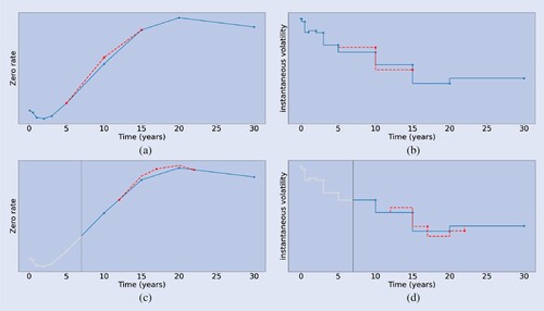
The sensitivities along the Monte Carlo path are understood as future-time generalizations of the quantities defined above. That is, future Delta ${\mathrm{\Delta }}_k\left(t\right)$ is interpreted as the sensitivity of $V_t$ to an infinitesimal bump of the hypothetical zero-rate node $R_k\left(t\right):=R(t,t+{\tau }_k)$, conditional on ${\mathcal{F}}_t$. This is graphically represented in figure 7(c). Future Vega ${\mathcal{V}}_k\left(t\right)$ is interpreted as the sensitivity of $V_t$ to an infinitesimal bump of the time-t implied volatility ${\sigma }_k\left(t\right):={\sigma }_{\mathrm{imp}}(t,t+{\tau }_k)$ corresponding to an ATM swaption maturing at $t+{\tau }_k$, conditional on ${\mathcal{F}}_t$. This is graphically represented in figure 7(d).

4.3. Computing the sensitivity

First we consider the general case and denote $\begin{array}{r}{\mathit{\theta }}_t:={\left({\theta }_1\right(t),{\theta }_2(t),\dots ,{\theta }_K(t\left)\phantom{|}\right)}^{\mathrm{\top }}\end{array}$ where either ${\theta }_k\left(t\right):=R_k\left(t\right)$ or ${\theta }_k\left(t\right):={\sigma }_k\left(t\right)$. Later on we will distinguish between the two cases. Without loss of generality, assume that $t\in (T_{m-1},T_m]$. The aim is to compute $\begin{array}{r}{D}_{\theta }\mathrm{\Pi }\left(t\right){|}_{\mathit{\theta }={\mathit{\theta }}_t}=\sum _{i=m}^{M-1}{D}_{\theta }{\mathrm{\Pi }}_i\left(t\right){|}_{\mathit{\theta }={\mathit{\theta }}_t}\end{array}$ We iteratively compute the sensitivities of each subportfolio, for $i=M-1,\dots ,m$. Starting with i = M−1, a static replication of $V_{T_{M-1}}$ is achieved with a single European swaption, i.e. ${\mathrm{\Pi }}_{M-1}:={\pi }_{M-1,1}$. Thus, setting $w_{M-1,1}=1$ and $K_{M-1,1}=K$. The Delta and Vega simply correspond to the sensitivities of a European swaption, i.e. $\begin{array}{r}{D}_{\theta }{\mathrm{\Pi }}_{M-1}\left(t\right)=(\frac{\mathrm{\partial }{\pi }_{M-1}\left(t\right)}{\mathrm{\partial }{\theta }_1},\dots ,\frac{\mathrm{\partial }{\pi }_{M-1}\left(t\right)}{\mathrm{\partial }{\theta }_K})\end{array}$ Next, consider the case i = m<M−1 and assume the sensitivities $D_{\theta }{\mathrm{\Pi }}_{m+1}\left(t\right),$ $\dots ,D_{\theta }{\mathrm{\Pi }}_{M-1}\left(t\right)$ are known. With slight abuse of notation, we have according to the chain rule the following relation (18) $\begin{array}{r}{D}_{\theta }{\mathrm{\Pi }}_m\left(t\right)=\underset{\begin{array}{c}\mathrm{options}\\ \mathrm{Delta}/\mathrm{Vega}\end{array}}{\underbrace{\frac{\mathrm{\partial }{\mathrm{\Pi }}_m\left(t\right)}{\mathrm{\partial }\mathit{\theta }}}}+\underset{\begin{array}{c}\mathrm{weight}\\ \mathrm{sensitivities}\end{array}}{\underbrace{\frac{\mathrm{\partial }{\mathrm{\Pi }}_m\left(t\right)}{\mathrm{\partial }{\mathit{w}}_{\mathit{m}}}\frac{\mathrm{\partial }{\mathit{w}}_{\mathit{m}}}{\mathrm{\partial }\mathit{\theta }}}}+\underset{\begin{array}{c}\mathrm{strike}\\ \mathrm{sensitivities}\end{array}}{\underbrace{\frac{\mathrm{\partial }{\mathrm{\Pi }}_m\left(t\right)}{\mathrm{\partial }{\mathit{k}}_{\mathit{m}}}\frac{\mathrm{\partial }{\mathit{k}}_{\mathit{m}}}{\mathrm{\partial }\mathit{\theta }}}}\end{array}$(18) We detail each term below:

Options Delta/Vega	The first term represents the standard Delta or Vega of the options composing the portfolio, i.e. (19) $\begin{array}{r}\frac{\mathrm{\partial }{\mathrm{\Pi }}_m\left(t\right)}{\mathrm{\partial }\mathit{\theta }}={\mathit{w}}_{\mathit{m}}^{\mathrm{\top }}{D}_{\theta }{\mathit{\pi }}_{\mathit{m}}\left(t\right)\end{array}$(19)
Weight sensitivities	The weights ${\mathit{w}}_{\mathit{m}}$ are optimized, such that the portfolio payoff matches a target function (equation (8(8) $\begin{array}{r}{f}_m\left(x\right)=\{\begin{array}{l}{q}_m\left(x\right)\cdot max\{h_m\left(x\right),0\}\\ \mathrm{if}m=M-1\\ q_m\left(x\right)\cdot max\{h_m\left(x\right)-{\tilde{C}}_m(T_m,x),0\}\\ \mathrm{if}m=M-2,\dots ,0\end{array}\end{array}$(8) )). This target function is sensitive to parameter changes in the zero-rate curve or volatility term-structure. As a consequence we need to consider the weight sensitivities, i.e. (20) $\begin{array}{r}\frac{\mathrm{\partial }{\mathrm{\Pi }}_m\left(t\right)}{\mathrm{\partial }{\mathit{w}}_{\mathit{m}}}\frac{\mathrm{\partial }{\mathit{w}}_{\mathit{m}}}{\mathrm{\partial }\mathit{\theta }}={\mathit{\pi }}_{\mathit{m}}^{\mathrm{\top }}\left(t\right)D_{\theta }{\mathit{w}}_{\mathit{m}}\end{array}$(20)
Strike sensitivities	For the same reason as for the weights, the sensitivities for the strikes should be considered. However, we conjecture the impact of the strike sensitivities is relatively small, which is supported by our numerical experiments. We will ignore this term for the remainder of this work.

A further derivation of the Delta/Vega sensitivities is the subject of sections 4.4 and 4.5. A further derivation of the weight sensitivities is subject of section 4.6.

4.4. The delta sensitivities

We start by working out the terms of the form $D_{\theta }{\mathit{\pi }}_{\mathit{m}}$ and consider the case ${\theta }_k\left(t\right)=R_k\left(t\right):=R(t,t+{\tau }_k)$. We perform the derivation for the general setting $0\le t\le T\le T_m$ and aim to compute $\begin{array}{r}{D}_{\theta }{\mathit{\pi }}_{\mathit{m}}\left(T\right){|}_{\mathit{\theta }={\mathit{\theta }}_t}=\left(\begin{array}{ccc}\frac{\mathrm{\partial }{\pi }_{m,1}\left(T\right)}{\mathrm{\partial }{R}_1\left(t\right)}& \dots & \frac{\mathrm{\partial }{\pi }_{m,1}\left(T\right)}{\mathrm{\partial }{R}_K\left(t\right)}\\ ⋮& \ddots & ⋮\\ \frac{\mathrm{\partial }{\pi }_{m,n}\left(T\right)}{\mathrm{\partial }{R}_1\left(t\right)}& \dots & \frac{\mathrm{\partial }{\pi }_{m,n}\left(T\right)}{\mathrm{\partial }{R}_K\left(t\right)}\end{array}\right)\end{array}$ The $D_{\theta }{\mathit{\pi }}_{\mathit{m}}$ in (19(19) $\begin{array}{r}\frac{\mathrm{\partial }{\mathrm{\Pi }}_m\left(t\right)}{\mathrm{\partial }\mathit{\theta }}={\mathit{w}}_{\mathit{m}}^{\mathrm{\top }}{D}_{\theta }{\mathit{\pi }}_{\mathit{m}}\left(t\right)\end{array}$(19) ) corresponds to the case t = T. The case t<T will serve as a path-wise sensitivity estimator, which will be required to compute the weight sensitivities in the subsequent section.

We first characterize the forward Delta sensitivity of a zero-coupon bond in the following lemma.

Lemma 4.1

Let $0\le t\le T_0\le T_1$ and assume that the zero-rate curve $\tau \mapsto R(t,t+\tau )$ is an interpolation between nodes $\left\{R_0\right(t),\dots ,R_K(t\left)\right\}$, where $R_k\left(t\right):=R(t,t+{\tau }_k)$. Then the forward Delta sensitivity is given by $\begin{array}{r}\frac{\mathrm{\partial }P(T_0,T_1)}{\mathrm{\partial }{R}_k\left(t\right)}={\alpha }_k({\tau }_0,{\tau }_1)P(T_0,T_1)\end{array}$ where ${\tau }_i=T_i-t$ and ${\alpha }_k$ denotes an ${\mathcal{F}}_t$-measurable coefficient, dependent on the interpolation scheme of the zero-rate nodes. If the interpolation is linear, the coefficient is given by $\begin{array}{rl}{\alpha }_k({\tau }_0,{\tau }_1)& :={\alpha }_k^{\mathrm{\prime }}\left({\tau }_1\right)-{\alpha }_k^{\mathrm{\prime }}\left({\tau }_0\right),\\ {\alpha }_k^{\mathrm{\prime }}\left(\tau \right)& :=\{\begin{array}{ll}{\displaystyle \frac{\tau -{\tau }_{k-1}}{{\tau }_k-{\tau }_{k-1}}\tau }& \mathrm{if}\tau \in ({\tau }_{k-1},{\tau }_k]\\ {\displaystyle \frac{{\tau }_{k+1}-\tau }{{\tau }_{k+1}-{\tau }_k}\tau }& \mathrm{if}\tau \in ({\tau }_k,{\tau }_{k+1}]\\ 0& \mathrm{otherwise}\end{array}\end{array}$

A proof to this lemma is given in appendix 1. Now, for brevity denote $H_{m,i}\left(t\right):={\mathbb{E}}^{m,M}\left[\right({\delta }_{m,i}\left(S_{m,M}\right(T_m)-K_{m,i})\phantom{|}{)}^{+}|{\mathcal{F}}_t]$. Then by an application of the chain rule and the product rule, we can write (21) $\begin{array}{rl}\frac{\mathrm{\partial }{\pi }_{m,i}\left(T\right)}{\mathrm{\partial }{R}_k\left(t\right)}& =A_{m,M}\left(T\right)\underset{\begin{array}{c}\mathrm{Bachelier}\\ \mathrm{Delta}\end{array}}{\underbrace{\frac{\mathrm{\partial }{H}_{m,i}\left(T\right)}{\mathrm{\partial }{S}_{m,M}\left(T\right)}}}\underset{\begin{array}{c}\mathrm{Swaprate}\\ \mathrm{sensitivity}\end{array}}{\underbrace{\frac{\mathrm{\partial }{S}_{m,M}\left(T\right)}{\mathrm{\partial }{R}_k\left(t\right)}}}\\ & +H_{m,i}\left(T\right)\underset{\begin{array}{c}\mathrm{Annuity}\\ \mathrm{sensitivity}\end{array}}{\underbrace{\frac{\mathrm{\partial }{A}_{m,M}\left(T\right)}{\mathrm{\partial }{R}_k\left(t\right)}}}\end{array}$(21) Working out each of the three partial derivatives above, we find

Bachelier Delta	Under the swap rate dynamics approximation given in (15(15) $\begin{array}{r}{S}_{m,M}\left(T\right)\approx {\tilde{S}}_{m,M}\left(T\right):=S_{m,M}\left(t\right)+{\int }_t^T{\tilde{\mathrm{\Sigma }}}_{m,M}\left(u{)}^{\mathrm{\top }}\eta \right(u)\cdot d{W}_u^{m,M}\end{array}$(15) ), this term is computed as the standard Bachelier Delta sensitivity, i.e. (22) $\begin{array}{rl}\frac{\mathrm{\partial }{H}_{m,i}\left(T\right)}{\mathrm{\partial }{S}_{m,M}\left(T\right)}& ={\delta }_{m,i}\mathrm{\Phi }\left({\delta }_{m,i}d\right),\\ d& =\frac{S_{m,M}\left(T\right)-K_{m,i}}{{\sigma }_{\mathrm{imp}}(T,T_m)\sqrt{T_m-T}}\end{array}$(22)
Annuity sensitivity	From Lemma 4.1 it directly follows $\begin{array}{rl}& \frac{\mathrm{\partial }{A}_{m,M}\left(T\right)}{\mathrm{\partial }{R}_k\left(t\right)}=\sum _{j=m+1}^M{\tau }_j{\alpha }_k(T-t,T_j-t)P(T,T_j)\end{array}$
Swap rate sensitivity	Applying the chain rule and Lemma 4.1, it follows $\begin{array}{rl}& \frac{\mathrm{\partial }{S}_{m,M}\left(T\right)}{\mathrm{\partial }{R}_k\left(t\right)}\\ & =\frac{\begin{array}{c}{\alpha }_k(T-t,T_m-t)P(T,T_m)-{\alpha }_k(T-t,T_m-t)\\ \times P(T,T_M)\end{array}}{A_{m,M}\left(T\right)}\\ & -S_{m,M}\left(T\right)\frac{\sum _{j=m+1}^M{\tau }_j{\alpha }_k(T-t,T_j-t)P(T,T_j)}{A_{m,M}\left(T\right)}\end{array}$

4.5. The vega sensitivities

Now consider the case ${\theta }_k\left(t\right)={\sigma }_k\left(t\right):={\sigma }_{\mathrm{imp}}(t,t+{\tau }_k)$. Just as for Delta, we perform the derivation for the general setting $0\le t\le T\le T_m$ and aim to compute $\begin{array}{r}{D}_{\theta }{\mathit{\pi }}_{\mathit{m}}\left(T\right){|}_{\mathit{\theta }={\mathit{\theta }}_t}=\left(\begin{array}{ccc}\frac{\mathrm{\partial }{\pi }_{m,1}\left(T\right)}{\mathrm{\partial }{\sigma }_1\left(t\right)}& \dots & \frac{\mathrm{\partial }{\pi }_{m,1}\left(T\right)}{\mathrm{\partial }{\sigma }_K\left(t\right)}\\ ⋮& \ddots & ⋮\\ \frac{\mathrm{\partial }{\pi }_{m,n}\left(T\right)}{\mathrm{\partial }{\sigma }_1\left(t\right)}& \dots & \frac{\mathrm{\partial }{\pi }_{m,n}\left(T\right)}{\mathrm{\partial }{\sigma }_K\left(t\right)}\end{array}\right)\end{array}$ Again, the $D_{\theta }{\mathit{\pi }}_{\mathit{m}}$ in (19(19) $\begin{array}{r}\frac{\mathrm{\partial }{\mathrm{\Pi }}_m\left(t\right)}{\mathrm{\partial }\mathit{\theta }}={\mathit{w}}_{\mathit{m}}^{\mathrm{\top }}{D}_{\theta }{\mathit{\pi }}_{\mathit{m}}\left(t\right)\end{array}$(19) ) corresponds to the case t = T. The case t<T will serve as a path-wise sensitivity estimator, which will be required to compute the weight sensitivities in the subsequent section.

We first characterize the forward implied volatility Vega in the following two lemmas.

Lemma 4.2

Let $S_{m,M}$ satisfy the Gaussian approximation of (15(15) $\begin{array}{r}{S}_{m,M}\left(T\right)\approx {\tilde{S}}_{m,M}\left(T\right):=S_{m,M}\left(t\right)+{\int }_t^T{\tilde{\mathrm{\Sigma }}}_{m,M}\left(u{)}^{\mathrm{\top }}\eta \right(u)\cdot d{W}_u^{m,M}\end{array}$(15) ) and denote $\tilde{\sigma }(t,T):=\sqrt{\frac{1}{T-t}{\int }_t^T\Vert {\mathrm{\Sigma }}_{m,M}^{\mathrm{\top }}\left(u\right)\eta \left(u\right){\Vert }_2^2\mathrm{d}u}$ for $0\le t\le T\le T_m$. Then $\begin{array}{rl}& \frac{\mathrm{\partial }{\sigma }_{\mathrm{imp}}(T,T_m)}{\mathrm{\partial }{\sigma }_k\left(t\right)}\\ & =\frac{(T_m-t)\tilde{\sigma }(t,T_m)\frac{\mathrm{\partial }\tilde{\sigma }(t,T_m)}{\mathrm{\partial }{\sigma }_k\left(t\right)}-(T-t)\tilde{\sigma }(t,T)\frac{\mathrm{\partial }\tilde{\sigma }(t,T)}{\mathrm{\partial }{\sigma }_k\left(t\right)}}{(T_m-T){\sigma }_{\mathrm{imp}}(T,T_m)}\end{array}$

A proof is given in appendix 2. The sensitivity of $\tilde{\sigma }(t,T)$ w.r.t. ${\sigma }_k\left(t\right)$ is an ${\mathcal{F}}_t$-measurable random variable, which is dependent on the calibration procedure of the instantaneous volatility $\eta \left(t\right)$. If ${\eta }_1,\dots ,{\eta }_K$ are scalars obtained by a bootstrap procedure, the sensitivities can be further characterized by the following lemma.

Lemma 4.3

Let $\eta \left(t\right)$ be scalar-valued and piece-wise constant. Let ${\mathrm{\Sigma }}_{m,M}$ be as in (14(14) $\begin{array}{rl}{\mathrm{\Sigma }}_{m,M}\left(t\right)& =B(t,T_M)\frac{P(t,T_M)}{A_{m,M}\left(t\right)}-B(t,T_m)\frac{P(t,T_m)}{A_{m,M}\left(t\right)}\\ & -S_{m,M}\left(t\right)\sum _{l=m+1}^M{\tau }_{l}B(t,T_l)\frac{P(t,T_l)}{A_{m,M}\left(t\right)}\end{array}$(14) ) and let ${\mathrm{\Sigma }}_k$ denote the diffusion of the swap rate underlying the option corresponding to ${\sigma }_k\left(t\right):={\sigma }_{\mathrm{imp}}(t,t+{\tau }_k)$. Then the forward implied volatility Vega is given by $\begin{array}{r}\frac{\mathrm{\partial }\tilde{\sigma }(t,T)}{\mathrm{\partial }{\sigma }_k\left(t\right)}={\alpha }_k\left(T\right)\frac{{\tau }_k{\sigma }_k\left(t\right)}{\tau \tilde{\sigma }(t,T)}\end{array}$ where $\tau :=T-t$ and ${\alpha }_k$ denotes an ${\mathcal{F}}_t$-measurable coefficient. If by approximation ${\mathrm{\Sigma }}_{m,M}\approx {\mathrm{\Sigma }}_k\approx {\mathrm{\Sigma }}_{k+1}$, the coefficient is given by $\begin{array}{r}{\alpha }_k\left(T\right)=\{\begin{array}{ll}{\displaystyle \frac{{\int }_{T_{k-1}}^T{\mathrm{\Sigma }}_{m,M}^2\left(u\right)\mathrm{d}u}{{\int }_{T_{k-1}}^{T_k}{\mathrm{\Sigma }}_k^2\left(u\right)\mathrm{d}u}}& \mathrm{if}{T}_{k-1}<T\le T_k\\ {\displaystyle \frac{{\int }_T^{T_{k+1}}{\mathrm{\Sigma }}_{m,M}^2\left(u\right)\mathrm{d}u}{{\int }_{T_k}^{T_{k+1}}{\mathrm{\Sigma }}_{k+1}^2\left(u\right)\mathrm{d}u}}& \mathrm{if}{T}_k<T\le T_{k+1}\\ 0& \mathrm{otherwise}\end{array}\end{array}$ where we denote $T_k:=t+{\tau }_k$.

A proof is given in appendix 3. By an application of the chain rule, we obtain (23) $\begin{array}{rl}\frac{\mathrm{\partial }{\pi }_{m,i}\left(T\right)}{\mathrm{\partial }{\sigma }_k\left(t\right)}& =\underset{\begin{array}{c}\mathrm{Bachelier}\\ \mathrm{Vega}\end{array}}{\underbrace{\frac{\mathrm{\partial }{\pi }_{m,i}\left(T\right)}{\mathrm{\partial }{\sigma }_{\mathrm{imp}}(T,T_m)}}}\underset{\begin{array}{c}\mathrm{Imp}.\mathrm{vol}.\\ \mathrm{sensitivity}\end{array}}{\underbrace{\frac{\mathrm{\partial }{\sigma }_{\mathrm{imp}}(T,T_m)}{\mathrm{\partial }{\sigma }_k\left(t\right)}}}\\ & +\underset{\begin{array}{c}\mathrm{Bachelier}\\ \mathrm{Delta}\end{array}}{\underbrace{\frac{\mathrm{\partial }{\pi }_{m,i}\left(T\right)}{\mathrm{\partial }{S}_{m,M}\left(T\right)}}}\underset{\begin{array}{c}\mathrm{Swaprate}\\ \mathrm{sensitivity}\end{array}}{\underbrace{\frac{\mathrm{\partial }{S}_{m,M}\left(T\right)}{\mathrm{\partial }{\sigma }_k\left(t\right)}}}\end{array}$(23) Considering each of the partial derivatives above, we find

• Bachelier Vega Under the swap rate approximation given in (15(15) $\begin{array}{r}{S}_{m,M}\left(T\right)\approx {\tilde{S}}_{m,M}\left(T\right):=S_{m,M}\left(t\right)+{\int }_t^T{\tilde{\mathrm{\Sigma }}}_{m,M}\left(u{)}^{\mathrm{\top }}\eta \right(u)\cdot d{W}_u^{m,M}\end{array}$(15) ), this term can be computed as the Bachelier Vega sensitivity, i.e. $\begin{array}{rl}\frac{\mathrm{\partial }{\pi }_{m,i}\left(T\right)}{\mathrm{\partial }{\sigma }_{\mathrm{imp}}(T,T_m)}& =A_{m,M}\left(T\right)\sqrt{T_m-T}\phi \left(d\right),\\ d& =\frac{S_{m,M}\left(T\right)-K_{m,i}}{{\sigma }_{\mathrm{imp}}(T,T_m)\sqrt{T_m-T}}\end{array}$

• Bachelier Delta Under the swap rate approximation given in (15(15) $\begin{array}{r}{S}_{m,M}\left(T\right)\approx {\tilde{S}}_{m,M}\left(T\right):=S_{m,M}\left(t\right)+{\int }_t^T{\tilde{\mathrm{\Sigma }}}_{m,M}\left(u{)}^{\mathrm{\top }}\eta \right(u)\cdot d{W}_u^{m,M}\end{array}$(15) ), this term can be computed as the Bachelier Delta sensitivity. Hence, similar to (22(22) $\begin{array}{rl}\frac{\mathrm{\partial }{H}_{m,i}\left(T\right)}{\mathrm{\partial }{S}_{m,M}\left(T\right)}& ={\delta }_{m,i}\mathrm{\Phi }\left({\delta }_{m,i}d\right),\\ d& =\frac{S_{m,M}\left(T\right)-K_{m,i}}{{\sigma }_{\mathrm{imp}}(T,T_m)\sqrt{T_m-T}}\end{array}$(22) ), we have (24) $\begin{array}{rl}\frac{\mathrm{\partial }{\pi }_{m,i}\left(T\right)}{\mathrm{\partial }{S}_{m,M}\left(T\right)}& ={\delta }_{m,i}{A}_{m,M}\left(T\right)\mathrm{\Phi }\left({\delta }_{m,i}d\right),\\ d& =\frac{S_{m,M}\left(T\right)-K_{m,i}}{{\sigma }_{\mathrm{imp}}(T,T_m)\sqrt{T_m-T}}\end{array}$(24)

• Imp. vol. sensitivity The forward implied volatility sensitivity is characterized in Lemma 4.2. Under the assumptions of Lemma 4.3, the sensitivity can be approximated as $\begin{array}{r}\frac{\mathrm{\partial }{\sigma }_{\mathrm{imp}}(T,T_m)}{\mathrm{\partial }{\hat{\sigma }}_k\left(t\right)}=\frac{\left(\phantom{|}{\alpha }_k\right(T_m)-{\alpha }_k(T\left)\right){\tau }_k{\sigma }_k\left(t\right)}{(T_m-T){\sigma }_{\mathrm{imp}}(T,T_m)}\end{array}$

• Swap rate sensitivity Under the swap rate approximation given in (15(15) $\begin{array}{r}{S}_{m,M}\left(T\right)\approx {\tilde{S}}_{m,M}\left(T\right):=S_{m,M}\left(t\right)+{\int }_t^T{\tilde{\mathrm{\Sigma }}}_{m,M}\left(u{)}^{\mathrm{\top }}\eta \right(u)\cdot d{W}_u^{m,M}\end{array}$(15) ), we can write $\begin{array}{r}{S}_{m,M}\left(T\right)\sim S_{m,M}\left(t\right)+\tilde{\sigma }(t,T)(W_T^{m,M}-W_t^{m,M})\end{array}$ where $\tilde{\sigma }(t,T):=\sqrt{\frac{1}{T-t}{\int }_t^T\Vert {\mathrm{\Sigma }}_{m,M}^{\mathrm{\top }}\left(u\right)\eta \left(u\right){\Vert }_2^2\mathrm{d}u}$. It follows that the forward swap rate sensitivity can be estimated as $\begin{array}{r}\frac{\mathrm{\partial }{S}_{m,M}\left(T\right)}{\mathrm{\partial }{\sigma }_k\left(t\right)}=\frac{S_{m,M}\left(T\right)-S_{m,M}\left(t\right)}{\tilde{\sigma }(t,T)}\frac{\mathrm{\partial }\tilde{\sigma }(t,T)}{\mathrm{\partial }{\sigma }_k\left(t\right)}\end{array}$ Under the assumptions of Lemma 4.3, this can be further approximated as $\begin{array}{r}\frac{\mathrm{\partial }{S}_{m,M}\left(T\right)}{\mathrm{\partial }{\sigma }_k\left(t\right)}=\frac{{\tau }_k{\alpha }_k\left(T\right)}{T-t}\left(S_{m,M}\right(T)-S_{m,M}(t\left)\phantom{|}\right)\end{array}$

4.6. The weight sensitivities

The weights and strikes of ${\mathrm{\Pi }}_m$ are obtained through an optimization scheme as described in section 3.1. The objective function for this optimization can equivalently be expressed as $\begin{array}{r}{L}_m(\mathit{w},\mathit{k})={\mathbb{E}}^{\mathbb{Q}}\left[{({\mathit{w}}^{\mathrm{\top }}{\mathit{\pi }}_{\mathit{m}}\left(T_m\right)-g_m\left(T_m\right))}^2\right]\end{array}$ where we denoted $g_m\left(t\right):=\frac{f_m\left(x_t\right)}{q_m\left(x_t\right)}$. The parameters ${\mathit{w}}_{\mathit{m}}$ and ${\mathit{k}}_{\mathit{m}}$ are determined by (25) $\begin{array}{r}({\mathit{w}}_{\mathit{m}},{\mathit{k}}_{\mathit{m}})={\arg \min }_{\mathit{w},\mathit{k}}\{L_m(\mathit{w},\mathit{k})|\mathit{w},\mathit{k}\in {\mathbb{R}}^n\}\end{array}$(25) Assuming $L_m$ attains a local minimum in $({\mathit{w}}_{\mathit{m}},{\mathit{k}}_{\mathit{m}})$, it follows by the first order optimality condition that $\mathrm{\nabla }{L}_m=\mathbf{0}$. In particular, we have $\begin{array}{r}{\lambda }_m\left({\mathit{w}}_{\mathit{m}}\right):=(\frac{\mathrm{\partial }{L}_m}{\mathrm{\partial }{w}_1},\dots ,\frac{\mathrm{\partial }{L}_m}{\mathrm{\partial }{w}_n}){|}_{\mathit{w}={\mathit{w}}_{\mathit{m}}}=\mathbf{0}\end{array}$ where we can compute $\begin{array}{rl}{\lambda }_m\left(\mathit{w}\right)& ={\mathbb{E}}^{\mathbb{Q}}\left[D_w{\left({\mathit{w}}^{\mathrm{\top }}{\mathit{\pi }}_{\mathit{m}}\right(T_m)-g_m(T_m\left)\right)}^2\right]\\ & =2{\mathbb{E}}^{\mathbb{Q}}\left[\left({\mathit{w}}^{\mathrm{\top }}{\mathit{\pi }}_{\mathit{m}}\right(T_m)-g_m(T_m\left)\right){\mathit{\pi }}_{\mathit{m}}\right(T_m\left)\right]\end{array}$ In order to characterize the weight sensitivities, we first consider the Jacobian of ${\lambda }_m$ (i.e. the Hessian of $L_m$ w.r.t. $\mathit{w}$). The Jacobian can be obtained by again differentiating the expression above, which yields (26) $\begin{array}{rl}{D}_w{\lambda }_m& =2{\mathbb{E}}^{\mathbb{Q}}\left[D_w\left({\mathit{w}}^{\mathrm{\top }}{\mathit{\pi }}_{\mathit{m}}\right(T_m)-g_m(T_m\left)\right){\mathit{\pi }}_{\mathit{m}}\right(T_m\left)\right]\end{array}$(26) (27) $\begin{array}{rl}& =2{\mathbb{E}}^{\mathbb{Q}}\left[{\mathit{\pi }}_{\mathit{m}}\right(T_m\left){\mathit{\pi }}_{\mathit{m}}^{\mathrm{\top }}\right(T_m\left)\right]\end{array}$(27) Hence, note that $D_w{\lambda }_m$ is specified by the auto-correlation matrix of the random vector ${\mathit{\pi }}_{\mathit{m}}$. In other words, it depends on the cross-sectional co-variance matrix of the portfolio payoffs. With this expression at hand, we characterize the weight sensitivities in the following proposition

Proposition 4.4

Consider a swaption portfolio ${\mathrm{\Pi }}_m$ written on swap rate $S_{m,M}$ and let its weights and strikes satisfy equation (25(25) $\begin{array}{r}({\mathit{w}}_{\mathit{m}},{\mathit{k}}_{\mathit{m}})={\arg \min }_{\mathit{w},\mathit{k}}\{L_m(\mathit{w},\mathit{k})|\mathit{w},\mathit{k}\in {\mathbb{R}}^n\}\end{array}$(25) ). Furthermore assume that the strikes $K_1,\dots ,K_n$ are all distinct. Then the derivative of ${\mathit{w}}_{\mathit{m}}$ w.r.t. ${\mathit{\theta }}_t$ is well-defined and its Jacobian matrix at $({\mathit{w}}_{\mathit{m}},{\mathit{\theta }}_t)$ is given by (28) $\begin{array}{r}\frac{\mathrm{\partial }{\mathit{w}}_{\mathit{m}}}{\mathrm{\partial }{\mathit{\theta }}_t}=-{\left(D_w{\lambda }_m\right)}^{-1}{D}_{\theta }{\lambda }_m{|}_{\mathit{w}={\mathit{w}}_{\mathit{m}},\mathit{\theta }={\mathit{\theta }}_t}\end{array}$(28)

This result is a consequence of the implicit function theorem. A rigorous proof is given in appendix 4.

Remark 1

The first term in (28(28) $\begin{array}{r}\frac{\mathrm{\partial }{\mathit{w}}_{\mathit{m}}}{\mathrm{\partial }{\mathit{\theta }}_t}=-{\left(D_w{\lambda }_m\right)}^{-1}{D}_{\theta }{\lambda }_m{|}_{\mathit{w}={\mathit{w}}_{\mathit{m}},\mathit{\theta }={\mathit{\theta }}_t}\end{array}$(28) ) is given by the inverse of the matrix in (27(27) $\begin{array}{rl}& =2{\mathbb{E}}^{\mathbb{Q}}\left[{\mathit{\pi }}_{\mathit{m}}\right(T_m\left){\mathit{\pi }}_{\mathit{m}}^{\mathrm{\top }}\right(T_m\left)\right]\end{array}$(27) ). Note that this term is both path-independent and time-independent. Hence, although its computation requires numerical estimation and matrix inversion, it can be used along each MC path, at each time-step without nested re-evaluation.

What remains to be done is computing $D_{\theta }{\lambda }_m$. We therefore compute $\begin{array}{rl}{D}_{\theta }{\lambda }_m& =2{\mathbb{E}}^{\mathbb{Q}}\left[{\mathit{\pi }}_{\mathit{m}}{D}_{\theta }\left({\mathit{w}}^{\mathrm{\top }}{\mathit{\pi }}_{\mathit{m}}\right(T_m)-g_m(T_m\left)\right)\right]\\ & +2{\mathbb{E}}^{\mathbb{Q}}\left[\left({\mathit{w}}^{\mathrm{\top }}{\mathit{\pi }}_{\mathit{m}}\right(T_m)-g_m(T_m\left)\right)D_{\theta }{\mathit{\pi }}_{\mathit{m}}\right(T_m\left)\right]\end{array}$ Note that the second term is zero if subportfolio ${\mathrm{\Pi }}_m$ yields a perfect fit to the target function $g_m$. Therefore, we can expect this term to be small and we will ignore it. Working out the first term, we find $\begin{array}{r}{D}_{\theta }{\lambda }_m\approx 2{\mathbb{E}}^{\mathbb{Q}}\left[{\mathit{\pi }}_{\mathit{m}}{\mathit{w}}^{\mathrm{\top }}{D}_{\theta }{\mathit{\pi }}_{\mathit{m}}\right(T_m\left)\right]-2{\mathbb{E}}^{\mathbb{Q}}\left[{\mathit{\pi }}_{\mathit{m}}{D}_{\theta }{g}_m\right(T_m\left)\right]\end{array}$ In the first term of the expression above, $D_{\theta }{\mathit{\pi }}_{\mathit{m}}\left(T_m\right)$ represent the Deltas/Vegas of subportfolio ${\mathrm{\Pi }}_m$. This term needs to be numerically estimated. The path-wise estimator has been derived in sections 4.4 and 4.5. The second term also needs to be numerically estimated. The path-wise estimator involves $D_{\theta }{g}_m\left(T_m\right)$, where $g_m\left(t\right):=\frac{f_m\left(x_t\right)}{q_m\left(x_t\right)}=max\left\{h_m\right(x_t)-\sum _{i=m+1}^{M-1}{\mathrm{\Pi }}_i(t),0\}$. Working out this term and denoting the event $E_m:=\left\{h_m\right(x_{T_m})>\sum _{i=m+1}^{M-1}{\mathrm{\Pi }}_i(T_m\left)\right\}$ yields (29) $\begin{array}{r}{D}_{\theta }{g}_m\left(T_m\right)={\mathbb{1}}_{E_m}{D}_{\theta }{h}_m\left(x_{T_m}\right)-{\mathbb{1}}_{E_m}\sum _{i=m+1}^{M-1}{D}_{\theta }{\mathrm{\Pi }}_i\left(T_m\right)\end{array}$(29) In the expression above, the term $D_{\theta }{h}_m\left(x_{T_m}\right)$ is equivalent to $D_{\theta }{\pi }_{m,0}\left(T_m\right)$ with $K_{m,0}=K$. The terms $D_{\theta }{\mathrm{\Pi }}_i\left(T_m\right)$ for $i=m+1,\dots ,M-1$ were assumed to be known from previous iterations.

4.7. The algorithms

Below we summarize the algorithms for composing the replicating portfolios (Algorithm 1) and computing the path-wise sensitivities (Algorithm 2). For the execution of the path-wise sensitivity algorithm, it is assumed that the static replication has been performed and subportfolios ${\mathrm{\Pi }}_0,\dots ,{\mathrm{\Pi }}_{M-1}$ have been derived from the trained parameters ${\text{β}}_0,\dots ,{\text{β}}_{M-1}$.

5. Numerical experiments

We demonstrate the performance of the algorithms presented in this work by considering several case studies. We select a one-factor Gaussian model with piece-wise constant instantaneous volatility to perform our numerical experiments (see Andersen and Piterbarg 2010). That is, we consider state-variable dynamics given by $\begin{array}{rl}\mathrm{d}{x}_t& =\left(\varphi \right(t)-a{x}_t)\mathrm{dt}+\eta \left(t\right)\mathrm{d}{W}_t,x_0=0\\ \varphi \left(t\right)& ={\int }_0^t{e}^{-2a(t-u)}\eta \left(u\right)\mathrm{d}u\\ r_t& =f(0,t)+x_t\end{array}$ where the scalar a denotes a constant mean-reversion rate, $W_t$ is a one-dimensional Brownian motion under $\mathbb{Q}$ and $f(t,T):=-\frac{\mathrm{\partial }\log R(t,T)}{\mathrm{\partial }T}$ denotes the instantaneous forward rate. The time-zero yield curve is assumed to be a linear interpolation between zero-rates with tenors ${\tau }_k$ as given in table 1. We consider a flat yield curve with all zero-rates equal to 3%. The instantaneous forward rate is assumed to be piece-wise constant between the tenor dates ${\tau }_k$. Each volatility level ${\eta }_k$ is bootstrapped against an ATM European payer swaption with maturity ${\tau }_k$ and implied volatility ${\sigma }_k$, such that ${\tilde{\sigma }}_{\mathrm{imp}}(0,{\tau }_k)={\sigma }_k$. All implied volatility targets ${\sigma }_k$ are set to 50 bps, resulting in the instantaneous volatilities presented in table 1. The mean-reversion rate is fixed a priori at a = 0.01. The tenors ${\tau }_k$ have been selected to coincide with the SIMM tenor buckets specified by ISDA (International Swaps and Derivatives Association, Inc 2020).

Table 1. Model parameters.

${\mathit{\tau }}_{\mathit{k}}$	2W	1M	3M	6M	1Y	2Y	3Y	5Y	10Y	15Y	20Y	30Y
${\mathit{R}}_{\mathit{k}}$	0.03	0.03	0.03	0.03	0.03	0.03	0.03	0.03	0.03	0.03	0.03	0.03
${\mathit{\eta }}_{\mathit{k}}$ (bps)	50.9	50.9	50.9	51.1	51.2	51.2	51.2	51.3	51.3	57.2	57.8	61.0

Sampling required for regression data, pricing, sensitivities, exposures and IM profiles is done using Monte Carlo simulation. The risk factor is simulated through an Euler discretization scheme. The discretization uses weekly time-steps, i.e. $\mathrm{\Delta t}=1/52$.

As case studies, we consider a $1Y\times 5Y$ and a $1Y\times 10Y$ Bermudan receiver swaption with unit notional. The underlying of the $T_0\times T_M$ Bermudan is assumed to be a fixed-for-floating interest rate swap with fixed rate K and a tenor structure $\mathcal{T}=\{T_0,\dots ,T_M\}$ of annual payments. Unless stated otherwise, the fixed rate K is selected to be ATM, i.e. $K=K_{\mathrm{ATM}}:=S_{0,M}\left(0\right)$. The exercise dates of the Bermudan are set to coincide with the fixing dates of the underlying swap, i.e. $T_0$ being the first and $T_{M-1}$ being the last exercise opportunity.

The composition of the static replication portfolio relies on the regression of feed-forward neural networks with a single hidden layer. Below, we list some details concerning the fitting procedure of the neural networks.

• As an independent regression variable for $G_m$ we select the swap rate $S_{m,M}\left(T_m\right)$. The regression data is normalized before $G_m$ is fitted to the data, to improve the regression robustness (see Hoencamp et al. 2023 for details).

• Each network $G_m$ is selected to have 8 hidden nodes.

• Each regression is performed with a data set of 2000 independently sampled training points.

• The neural network parameters are optimized using the AdaMax optimizer, which is a stochastic gradient-descent method (Kingma and Ba 2014). The batch-size (i.e. number of training points used per iteration) is set to 32. The learning rate (i.e. the step-size scaling per iteration) is set to 0.01.

• The parameters of $G_{M-1}$ are randomly initialized from a uniform distribution $\mathcal{U}(-1,1)$. For m<M−1, the parameters of $G_m$ are initialized with the optimized parameters of $G_{m+1}$.

5.1. Pricing

We start by analyzing the pricing accuracy of the static replication. As each neural network has 8 hidden nodes, every regression yields a subportfolio of 8 European swaptions. Hence at t-zero, the $1Y\times 5Y$ Bermudan is replicated with 40 swaptions and the $1Y\times 10Y$ Bermudan is replicated with 80 swaptions.

5.1.1. Time-zero prices

Table 2 reports the $V_0$ price estimates implied by the risk-neutral valuation of the static replication portfolio (SR) for different levels of moneyness. As a benchmark, we report price estimates obtained from the least-square method (LSM) introduced by Longstaff and Schwartz (2001). As basis functions for the ordinary least-square regression, we use $\{1,x_t,x_t^2,x_t^3\}$. The LSM estimate is the mean of 25 independent runs of 80 000 MC paths each. In brackets, we report the standard error generated by these 25 runs.

Table 2. $V_0$ estimates Bermudan swaption for different levels of moneyness, presented in basis points of the notional.

	$1Y\times 5Y$		$1Y\times 10Y$
$K/S_{0,M}$	SR	LSM (SE)	SR	LSM (SE)
60%	14.43	14.18 (0.15)	61.04	60.20 (0.48)
80%	46.63	46.63 (0.35)	140.7	139.9 (0.8)
100%	130.4	130.3 (0.5)	300.5	300.2 (1.2)
120%	300.4	300.6 (0.7)	590.6	590.2 (1.4)
140%	543.8	544.6 (0.9)	1018.3	1018.8 (1.6)

From table 2, we observe a close correspondence between SR and LSM, in particular for ATM strikes. The accuracy slightly deteriorates for far OTM options. This can be attributed to a limited number of ITM paths at future monitor dates, yielding only a few non-zero data-points for the regression. SR is not subject to a standard error as the portfolios are evaluated at t-zero. SR is however subject to numerical errors due to the inaccuracy of the neural network regression. On the normalized data, the fits typically show a mean squared error in the order of ${10}^{-6}-{10}^{-5}$.

5.1.2. Exposure profiles

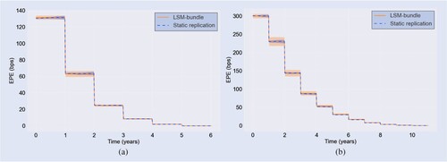
Consecutively, we consider the exposure profile and related CVA quantities of the Bermudan swaptions. Exposure depends on the future distribution of the option price. Figure 8 shows the expected positive exposure (EPE) simulated with the static replication next to an LSM implied benchmark. The benchmark is generated with the LSM-bundle algorithm, presented in Feng et al. (2016). We briefly summarize this method below.

Figure 8. Expected positive exposure profile: LSM-bundle (orange) vs. static replication (blue). The LSM and static replication standard error windows are represented by the orange and blue shaded area, respectively, based on 25 independent runs of 3000 MC paths. (a) $1Y\times 5Y$ Bermudan and (b) $1Y\times 10Y$ Bermudan.

The LSM-bundle algorithm allows one to estimate the EPE of a Bermudan option when combined with the LSM algorithm of Longstaff and Schwartz (2001). Within LSM, the continuation value $C_m\left(T_m\right)$ is estimated by regressing realized (discounted) cashflows at $T_{m+1}$ against the risk-factor realizations at $T_m$ on in-the-money MC paths. However, to compute the exposure, an unbiased estimate of the continuation value is required on each MC path on every exposure date (not just monitor dates). In Feng et al. (2016) it is therefore proposed to first perform an LSM sweep. Then in a second sweep, for each exposure date t the MC paths are divided into two bundles. If $t\in (T_{m-1},T_m]$, the two bundles are defined as: $\begin{array}{r}{\mathcal{U}}_1\left(t\right):=\{x_t:h_m(x_t)>0\},{\mathcal{U}}_2\left(t\right):=\{x_t:h_m(x_t)\le 0\}\end{array}$ Subsequently for both bundles an ordinary least-square regression is performed against the discounted realized cashflows that were computed in the first LSM sweep. The regression functions provide an unbiased estimate of the exposure for a given realization of the risk-factor in their respective domains. We refer to Feng et al. (2016) for details. Note that for the SR method, no second sweep of regressions is required. Exposures are obtained by simply pricing the replicating portfolio along the MC path.

The EPE profiles in figure 8 represent the mean of 25 MC simulations of 3000 paths each. The shaded areas represent a window of one standard error for both respective methods. We observe the typical staircase nature that corresponds to the exposure profile of a Bermudan option. Each discontinuity represents the passing of an exercise opportunity, after which the option is exercised for a certain fraction of the scenarios. Similar to the time-zero prices, we observe a good correspondence between the SR estimates and the benchmark. Additionally, it is noted that the standard error for SR is significantly smaller compared to LSM-bundle. This can be attributed to the benefit of the regress-later approach of SR compared to the regress-now approach of LSM. In the latter, the continuation value is estimated by regressing the (noisy) realizations of the cashflow. In the former, the regression is performed against the deterministic option's target value (numerical errors aside). As a result, the MC noise is integrated out more efficiently with SR. In general, this indicates that a significantly smaller number of MC paths would be required to reach a similar level of accuracy.

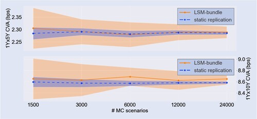
We further study the convergence of the standard error, by considering the CVA statistic. To do so, we assume a constant LGD = 1 and constant hazard rate of $\lambda \left(t\right)=0.01$. The CVA is estimated using equation (3(3) $\begin{array}{rl}\mathrm{CVA}& =(1-\mathrm{RR}){\int }_0^T\mathrm{EPE}\left(u\right)\mathrm{d}\mathbb{Q}(\tau =u)\\ & \approx \mathrm{LGD}\sum _{i=1}^n\mathrm{EPE}\left(t_i\right)\times \mathrm{PD}(t_{i-1},t_i)\end{array}$(3) ). Figure 9 shows the mean and standard deviation of the CVA estimate generated with 25 independent MC runs, as a function of the number of MC paths per run. We observe that on average the SR standard error is a factor 4 smaller compared to the LSM-bundle benchmark. For an increasing number of paths, the two methods show a consistent convergence.

Figure 9. Convergence CVA for a $1Y\times 5Y$ (top) and $1Y\times 10Y$ (bottom) Bermudan swaption: LSM-bundle (orange) vs. static replication (blue). The LSM and static replication standard error windows are represented by the orange and blue shaded area, respectively.

5.2. Sensitivities

We continue by analyzing the accuracy in the sensitivity computation for the static replication. We distinguish between time-zero sensitivities and future sensitivities along the MC path. The Delta and Vega sensitivities in this section are understood in accordance with the definitions provided in section 4.2.

5.2.1. Time-zero sensitivities

Figure 10 reports the time-zero Delta sensitivities for the 12 tenor buckets. The sensitivities have been scaled to represent the basis point value w.r.t. the zero-rate $R_k$. The SR results (presented in blue) are calculated in accordance with the Delta routine described in section 4.2. As a benchmark, we consider an LSM bump-and-reval estimate (presented in orange). For Delta, this means a zero-rate corresponding to one of the predefined tenors is bumped with one basis point and the yield curve is re-interpolated accordingly. The same seed is used for the LSM base run as for the bumped LSM run, to facilitate variance reduction.

Figure 10. Bucketed Delta sensitivities: LSM bump-and-reval (orange) vs. static replication (blue). The LSM benchmark is based on 25 independent runs of 80,000 MC paths. (a) $1Y\times 5Y$ Bermudan and (b) $1Y\times 10Y$ Bermudan.

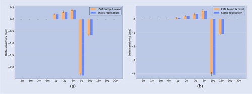
Figure 11 reports the time-zero Vega sensitivities for the 12 tenor buckets. These sensitivities have been scaled to represent the basis point value w.r.t. implied volatility ${\sigma }_k$. The bump-and-reval benchmark for Vega is obtained by bumping one of the implied volatilities with one basis point and re-bootstrapping the volatilty term-structure accordingly. Also here the same seed is used for the base and the bumped LSM run.

Figure 11. Bucketed Vega sensitivities: LSM bump-and-reval (orange) vs. static replication (blue). The LSM benchmark is based on 80,000 MC paths. (a) $1Y\times 5Y$ Bermudan and (b) $1Y\times 10Y$ Bermudan.

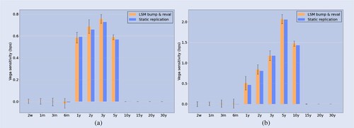
The results shown is figures 10 and 11 are the mean of 25 independent runs of 80,000 paths each. For the LSM bump-and-reval, this means 13 LSM simulations were involved for each run (1 base simulation and 12 bumped simulations). The SR estimate only requires a single simulation, in order to estimate the weight sensitivities of the replicating portfolio. The swaption sensitivities can be readily evaluated. The error bars indicate the standard error of the LSM estimate. The SR standard errors were each 2 to 3 orders of magnitude smaller compared to LSM and are therefore not included in the figures. Overall, we observe a satisfactory correspondence between the SR sensitivities and the LSM benchmark. For the LSM Vega, we observe relatively large standard errors compared to Delta. This can be attributed to the fact that a bumped yield curve translates one-to-one into bumped zero-coupon bond prices. A bumped volatility term-structure only indirectly impacts the risk-factor distribution and is therefore more susceptible to a higher standard error.

Table 3 reports the SIMM Delta, Vega and Curvature margins computed with the sensitivity estimates of SR and LSM, respectively, for different levels of moneyness. In brackets we report the standard error of the LSM implied quantities. For the Delta and Vega margin estimates, we see the accuracy of the SR method confirmed. The Curvature margin LSM estimates demonstrate a significantly larger standard error in the relative sense. Curvature margin reflects the Gamma sensitivity of the option, which in SIMM is approximated through a Vega-Gamma relationship (International Swaps and Derivatives Association, Inc 2016). Second-order sensitivity approximations are notorious for amplifying numerical errors of the first order sensitivities, which we see reflected in the LSM benchmark. The SR estimate does not suffer from such standard errors.

Table 3. IM estimate Bermudan swaption.

		$1Y\times 5Y$		$1Y\times 10Y$
$K/S_{0,M}$	Margin	SR	LSM (SE)	SR	LSM (SE)
60%	Delta	17.44	17.09 (1.19)	53.45	51.70 (4.07)
	Vega	7.81	8.09 (0.43)	26.01	26.34 (1.84)
	Curv.	1.12	1.42 (0.84)	2.20	3.57 (3.22)
80%	Delta	49.07	47.51 (2.91)	112.1	107.0 (6.9)
	Vega	14.93	15.54 (0.62)	38.98	39.28 (1.79)
	Curv.	2.75	2.91 (1.63)	4.23	4.10 (3.62)
100%	Delta	115.2	111.9 (3.8)	213.4	211.3 (14.7)
	Vega	19.56	20.04 (1.00)	45.46	46.58 (3.34)
	Curv.	5.06	5.61 (2.8)	7.21	8.79 (6.42)
120%	Delta	200.5	198.3 (4.7)	355.7	355.5 (14.5)
	Vega	12.84	12.80 (1.13)	33.58	34.22 (3.55)
	Curv.	4.29	3.63 (2.96)	8.03	10.84 (8.99)
140%	Delta	247.3	246.7 (2.4)	464.0	463.1 (10.0)
	Vega	2.92	3.09 (0.74)	10.54	10.61 (2.57)
	Curv.	1.11	1.58 (1.55)	3.27	4.82 (5.37)

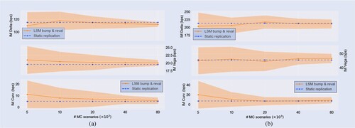
The convergence of the margin estimates is demonstrated in figure 12. Here we present the mean and standard error as a function of the number of MC paths, obtained from 25 independent runs. We observe that the consistency of the SR method is confirmed for an increasing number of MC paths.

Figure 12. Convergence Delta (top), Vega (middle) and Curvature (bottom) IM: LSM bump-and-reval (orange) vs. static replication (blue). The LSM standard error window is represented by the shaded orange area. (a) $1Y\times 5Y$ Bermudan and (b) $1Y\times 10Y$ Bermudan.

Figure 13. Bucketed Delta (left) and Vega (right) profiles for static replication of a European $5Y\times 5Y$ swaption. SR sensitivities (solid) are shown next to an exact benchmark (dashed). (a) Delta profiles and (b) Vega profiles.

5.2.2. Future sensitivities: European swaption

We finally analyze the expected future sensitivity profiles of a Bermudan swaption. Calculation of expected future sensitivities through the LSM bump-and-reval method would impose a severe computational burden. A nested MC simulation is required for each time-step, on each MC path, for each sensitivity. Benchmarking future sensitivity profiles is hence not feasible with LSM and out of scope for this paper.

To verify the accuracy of the SR method along the MC path, we therefore start by considering a $5Y\times 5Y$ European payer swaption. This can be considered a special case of the Bermudan, with only a single exercise opportunity at $T_0$. We proceed to replicate this swaption, while selecting the $15Y$ swap rate as regression asset. As a result, the $5Y\times 5Y$ swaption is replicated with a portfolio of $5Y\times 15Y$ swaptions. The same neural network structure is used as for the Bermudans. Subsequently, we analyze the sensitivity profiles of the replicating portfolio, which we benchmark with the analytical sensitivities of the swaption.

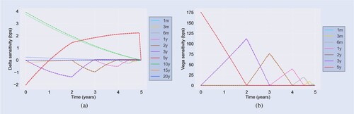
The results are displayed in figure 13. The Vega profiles on the right show a near-perfect match between SR and the benchmark. We do observe some numerical errors in the Delta $10Y$, $15Y$ and $20Y$ buckets. Around t = 0, the latter two are dominant for the $5Y\times 15Y$ swaptions in the replicating portfolio, but zero for the target $5Y\times 5Y$ swaption. If the replication is perfect, the sensitivities in this bucket cancel with the weight sensitivities. Here we note that some small errors remain. Yet, overall, we observe a satisfactory agreement between SR and the analytical profiles.

5.2.3. Future sensitivities: Bermudan swaption

Figure 14 shows the expected future Delta sensitivity profiles of a Bermudan swaption. The profiles are generated by taking the mean of 25 independent MC runs of 3000 paths each. The shaded areas (where visible) represent a single standard error window. As the underlying is a receiver swap, we note that the Delta profiles are mostly negative. The tenor buckets surrounding the time until maturity of the underlying swap are dominant. As time passes, the time to maturity decreases and the dominant sensitivities shift from one bucket to the next, implying the triangular-shaped profiles. We see this for example reflected in the (red-colored) Delta-profile of the $5Y$ bucket in figure 14(a). In the first year, the sensitivity grows (in the absolute sense) to its maximum until the maturity of the underlying swap is exactly $5Y$ away. Then, the sensitivity of this bucket starts to drop and flows into the $3Y$ bucket. The discontinuous jumps signify the passing of an exercise opportunity. Despite the small number of paths, we observe a satisfactory low standard error.

Figure 14. Bucketed Delta profiles for static replication. The standard error windows are represented by the shaded area, based on 3000 MC paths. (a) $1Y\times 5Y$ Bermudan and (b) $1Y\times 10Y$ Bermudan.

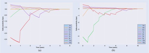
Figure 15 shows the corresponding expected Vega profiles and their standard error window. The sensitivities are scaled by the implied volatility in basis points of each corresponding bucket, which is in line with the SIMM routines. The Vega sensitivities are bucketed according to their time to expiry. Hence, we observe triangular patterns resulting from Vegas shifting from one bucket into the next as the time until the future monitor dates decreases. Also here, we observe that the shaded areas representing the standard errors are minor or even invisible in the figure, even though the number of paths is relatively small.

Figure 15. Bucketed Vega profiles for static replication. The standard error windows are represented by the shaded area, based on 3000 MC paths. (a) $1Y\times 5Y$ Bermudan and (b) $1Y\times 10Y$ Bermudan.

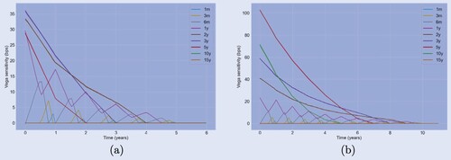
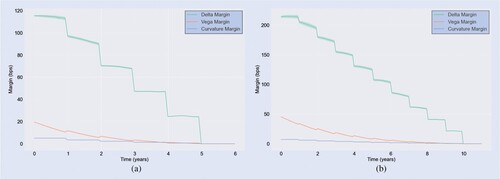
Figure 16 shows the expected initial margin profiles, obtained from the simulated sensitivity distributions. The shaded areas again denote a single standard error window. The figure shows the separate profiles corresponding the Delta-, Vega- and Curvature margin. The sum of these three yields the total expected initial margin as a function of time. From this plot, we observe that overall the Delta margin is dominant for the computation of IM and MVA. For Delta, we observe the typical staircase profile. Each discontinuity represents the passing of an exercise date and the subsequent decrease in the option's total Delta sensitivity. The volume of Vega scales with the square root of the times until expiry of the underlying options. Hence the smooth decay of the Vega margin over time, with similar jumps after each monitor date. The contribution of the curvature margin to the total IM and MVA is very limited. In terms of shape, the profile shows a similar nature as Delta.

Figure 16. Delta (green), Vega (orange) and Curvature (blue) margin profiles for static replication. The standard error windows are represented by the shaded area, based on 3000 MC paths. (a) $1Y\times 5Y$ Bermudan and (b) $1Y\times 10Y$ Bermudan.

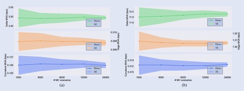
We study the convergence of the margin estimates by considering MVA as a function of the number of MC paths. Figure 17 shows the Delta-, Vega- and Curvature components of MVA in separate plots. We report the mean and standard error, obtained from 25 independent runs. The MVA estimates have been generated from the future IM distributions, while assuming a constant funding spread of $\mathrm{FS}\left(t\right)=0.01$. From the figures, we observe a consistent convergence and see the low standard errors of the sensitivity profiles confirmed. We conclude that generally, 3000 MC paths suffice to guarantee a relative standard error of below 1%.

Figure 17. Convergence Delta (top), Vega (middle) and Curvature (bottom) MVA for static replication. The standard error windows are represented by the shaded areas. (a) $1Y\times 5Y$ Bermudan and (b) $1Y\times 10Y$ Bermudan.

6. Conclusion

This paper presented a static replication algorithm for Bermudan swaptions under an affine term-structure model. We showed that under the appropriate conditions, one can construct a portfolio of European swaptions that mirrors the value of the exotic instrument until it is either exercised or matured. This replication is static, i.e. despite the early-exercise features of the instrument, the portfolio does not need to be re-balanced throughout the lifetime of the original contract. We continued to derive efficient estimators for the price and sensitivities of the portfolio along the Monte Carlo path. These quantities are essential for the quantification of modern risk metrics such as exposure, CVA, IM and MVA. Exploiting closed-form price and sensitivity approximations for European swaptions allowed us to avoid cumbersome nested simulations that are associated with a naive bump-and-reval approach. Moreover, this enabled us to accurately estimate high dimensional, bucketed Delta- and Vega sensitivities, despite the fact that the risk-factors may be embedded in a low dimensional model. This yielded a richer handle for sensitivity modeling compared to, for example, a parallel shift in the model variables. Through several representative numerical examples, we demonstrated the performance of our approach under a one-factor model, benchmarked to the established least-square Monte Carlo method of Longstaff and Schwartz (2001). Overall, we observed superior convergence for the static replication method with regard to exposures, sensitivities and IM statistics. Thus, we demonstrated static replication to be a suitable alternative for exposure, dynamic IM and MVA quantification.

Disclosure statement

The opinions expressed in this work are solely those of the authors and do not represent in any way those of their current and past employers. No potential conflict of interest was reported by the authors.

Additional information

Funding

This project has received funding from the NWO under the Industrial Doctorates grant.

Notes

1 For simplicity we will ignore the zero-coupon bond in the replicating portfolio (see section 3.2). This is achieved by constraining $b_2=0$. Our numerical experiments indicate a minimal impact on the accuracy of the replication.

Appendices

Appendix 1.

Proof of Lemma 4.1

Proof.

Consider the process $\begin{array}{r}{y}_t:=\frac{P(t,T_1)}{P(t,T_0)}\end{array}$ As y represents a tradable asset denominated by the numéraire, it follows that y is a Martingale under ${\mathbb{Q}}^{T_0}$. An application of Itô's lemma and a subsequent measure change shows that y satisfies the following SDE $\begin{array}{r}\mathrm{d}{y}_t=y_t{\left(B\right(t,T_0)-B(t,T_1\left)\right)}^{\mathrm{\top }}\eta \left(t\right)\mathrm{d}{W}_t^{T_0}\end{array}$ where $W^{T_0}$ denotes a d-dimensional Brownian motion under ${\mathbb{Q}}^{T_0}$. Denoting $\hat{\eta }\left(t\right):=\left(B\right(t,T_0)-B(t,T_1\left){)}^{\mathrm{\top }}\eta \right(t)$ and solving the SDE, conditioned on ${\mathcal{F}}_t$ yields $\begin{array}{r}P(T_0,T_1):=y_{T_0}=\frac{P(t,T_1)}{P(t,T_0)}{e}^{{\int }_t^{T_0}\hat{\eta }\left(u\right)\mathrm{d}{W}_u^{T_0}}\end{array}$ Let ${\tau }_0=T_0-t$ and ${\tau }_1=T_1-t$. Note that by the definition of the zero-rate, the expression above can be rewritten as $\begin{array}{r}P(T_0,T_1)=\exp \left\{{\tau }_{0}R\right(t,t+{\tau }_0)-{\tau }_{1}R(t,t+{\tau }_1)+{\int }_t^{T_0}\hat{\eta }(u\left)\mathrm{d}{W}_u^{T_0}\right\}\end{array}$ Therefore, the forward Delta sensitivity can be computed as $\begin{array}{r}\frac{\mathrm{\partial }P(T_0,T_1)}{\mathrm{\partial }{R}_k\left(t\right)}=({\tau }_0\frac{\mathrm{\partial }R(t,t+{\tau }_0)}{\mathrm{\partial }{R}_k\left(t\right)}-{\tau }_1\frac{\mathrm{\partial }R(t,t+{\tau }_1)}{\mathrm{\partial }{R}_k\left(t\right)})P(T_0,T_1)\end{array}$ where ${\alpha }_k^{\mathrm{\prime }}\left({\tau }_i\right):={\tau }_i\frac{\mathrm{\partial }R(t,t+{\tau }_i)}{\mathrm{\partial }{R}_k\left(t\right)}$ denotes an ${\mathcal{F}}_t$-measurable coefficient. Under the assumption that the time-t zero-rate curve $\tau \mapsto R(t,t+\tau )$ is an interpolation between nodes $\left\{R_0\right(t),\dots ,R_K(t\left)\right\}$, it follows that $\begin{array}{r}\frac{\mathrm{\partial }R(t,t+{\tau }_0)}{\mathrm{\partial }{R}_k\left(t\right)}=\{\begin{array}{ll}{\displaystyle \frac{\tau -{\tau }_{k-1}}{{\tau }_k-{\tau }_{k-1}}}& \mathrm{if}\tau \in ({\tau }_{k-1},{\tau }_k]\\ {\displaystyle \frac{{\tau }_{k+1}-\tau }{{\tau }_{k+1}-{\tau }_k}}& \mathrm{if}\tau \in ({\tau }_k,{\tau }_{k+1}]\\ 0& \mathrm{otherwise}\end{array}\end{array}$ This concludes the proof.

Appendix 2.

Proof of Lemma 4.2

Proof.

Let $0\le t\le T\le T_m$. Note that we can write $\begin{array}{rl}& {\sigma }_{\mathrm{imp}}(T,T_m)\\ & =\sqrt{\frac{1}{T_m-T}{\int }_T^{T_m}\Vert {\tilde{\mathrm{\Sigma }}}_{m,M}^{\mathrm{\top }}\left(u\right)\eta \left(u\right){\Vert }_2^2\mathrm{d}u}\\ & =\sqrt{\frac{1}{T_m-T}({\int }_t^{T_m}\Vert {\tilde{\mathrm{\Sigma }}}_{m,M}^{\mathrm{\top }}(u\left)\eta \right(u){\Vert }_2^2\mathrm{d}u-{\int }_t^T\Vert {\tilde{\mathrm{\Sigma }}}_{m,M}^{\mathrm{\top }}(u\left)\eta \right(u\left){\Vert }_2^2\mathrm{d}u\right)}\\ & =\frac{1}{\sqrt{T_m-T}}\sqrt{(T_m-t){\tilde{\sigma }}^2(t,T_m)-(T-t){\tilde{\sigma }}^2(t,T)}\end{array}$ Subsequently applying the chain rule to this expression yields $\begin{array}{rl}\frac{\mathrm{\partial }{\sigma }_{\mathrm{imp}}(T,T_m)}{\mathrm{\partial }{\sigma }_k\left(t\right)}& =\frac{1}{\sqrt{T_m-T}}\frac{(T_m-t)\frac{\mathrm{\partial }{\tilde{\sigma }}^2(t,T_m)}{\mathrm{\partial }{\sigma }_k\left(t\right)}-(T-t)\frac{\mathrm{\partial }{\tilde{\sigma }}^2(t,T)}{\mathrm{\partial }{\sigma }_k\left(t\right)}}{2\sqrt{(T_m-t){\tilde{\sigma }}^2(t,T_m)-(T-t){\tilde{\sigma }}^2(t,T)}}\\ & =\frac{(T_m-t)\tilde{\sigma }(t,T_m)\frac{\mathrm{\partial }\tilde{\sigma }(t,T_m)}{\mathrm{\partial }{\sigma }_k\left(t\right)}-(T-t)\tilde{\sigma }(t,T)\frac{\mathrm{\partial }\tilde{\sigma }(t,T)}{\mathrm{\partial }{\sigma }_k\left(t\right)}}{(T_m-T){\tilde{\sigma }}_{\mathrm{imp}}(T,T_m)}\end{array}$ This concludes the proof.

Appendix 3.

Proof of Lemma 4.3

Proof.

Recall that it is assumed that the instantaneous volatility in (1(1) $\begin{array}{r}\mathrm{d}{x}_t=\mu (t,x_t)\mathrm{d}t+\eta \left(t\right)\mathrm{d}{W}_t\end{array}$(1) ) takes values in $\mathbb{R}$ and is piece-wise constant between dates $\{{\tau }_0,\dots ,{\tau }_K\}$. Furthermore it is assumed that the volatility levels ${\eta }_1,\dots ,{\eta }_K$ are obtained through a bootstrap procedure, such that the implied volatility approximations ${\tilde{\sigma }}_{\mathrm{imp}}$ given in (17(17) $\begin{array}{rl}& =\sqrt{\frac{1}{T-t}{\int }_t^T\Vert {\tilde{\mathrm{\Sigma }}}_{m,M}\left(u{)}^{\mathrm{\top }}\eta \right(u){\Vert }_2^2\mathrm{d}u}\end{array}$(17) ) agree with the implied volatilities ${\sigma }_k$ observed in the market. Lastly, note that only ${\eta }_k$ and ${\eta }_{k+1}$ are sensitive to a change in ${\sigma }_k$ if other market-implied volatilities are kept fixed. For compactness of notation, we show the proof for t = 0. The generalization to t>0 follows the same line of thought.

First consider the case ${\tau }_{k-1}\le T<{\tau }_k$. Note that we can write (A1) $\begin{array}{rl}{\tau }_k{\sigma }_k^2& ={\int }_0^{T_{k-1}}{\mathrm{\Sigma }}_k^2\left(u\right){\eta }^2\left(u\right)\mathrm{d}u+{\eta }_k^2{\int }_{T_{k-1}}^{T_k}{\mathrm{\Sigma }}_k^2\left(u\right)\mathrm{d}u\\ ⟹{\eta }_k^2& =\frac{{\tau }_k{\sigma }_k^2-{\int }_0^{T_{k-1}}{\mathrm{\Sigma }}_k^2\left(u\right){\eta }^2\left(u\right)\mathrm{d}u}{{\int }_{T_{k-1}}^{T_k}{\mathrm{\Sigma }}_k^2\left(u\right)\mathrm{d}u}\end{array}$(A1) Furthermore, we have the relation $\begin{array}{r}\tilde{\sigma }(0,T)=\sqrt{\frac{1}{T}\left({\int }_0^{T_{k-1}}{\mathrm{\Sigma }}_{m,M}^2\right(u\left){\eta }^2\right(u)\mathrm{d}u+{\eta }_k^2{\int }_{T_{k-1}}^T{\mathrm{\Sigma }}_{m,M}^2(u\left)\mathrm{d}u\right)}\end{array}$ It follows by the chain rule $\begin{array}{rl}\frac{\mathrm{\partial }\tilde{\sigma }(0,T)}{\mathrm{\partial }{\sigma }_k}& =\frac{1}{2\tilde{\sigma }(0,T)}\frac{1}{T}\frac{\mathrm{\partial }}{\mathrm{\partial }{\sigma }_k}\\ & \times \left({\int }_0^{T_{k-1}}{\mathrm{\Sigma }}_{m,M}^2\right(u\left){\eta }^2\right(u)\mathrm{d}u+{\eta }_k^2{\int }_{T_{k-1}}^T{\mathrm{\Sigma }}_{m,M}^2(u\left)\mathrm{d}u\right)\\ & =\frac{1}{2T\tilde{\sigma }(0,T)}\left({\int }_{T_{k-1}}^T{\mathrm{\Sigma }}_{m,M}^2\right(u\left)\mathrm{d}u\right)\frac{\mathrm{\partial }{\eta }_k^2}{\mathrm{\partial }{\sigma }_k}\\ & =\frac{{\tau }_k{\sigma }_k}{T\tilde{\sigma }(0,T)}\frac{{\int }_{T_{k-1}}^T{\mathrm{\Sigma }}_{m,M}^2\left(u\right)\mathrm{d}u}{{\int }_{T_{k-1}}^{T_k}{\mathrm{\Sigma }}_k^2\left(u\right)\mathrm{d}u}\end{array}$ where the last equality follows from substituting ${\eta }_k^2$ with (A1(A1) $\begin{array}{rl}{\tau }_k{\sigma }_k^2& ={\int }_0^{T_{k-1}}{\mathrm{\Sigma }}_k^2\left(u\right){\eta }^2\left(u\right)\mathrm{d}u+{\eta }_k^2{\int }_{T_{k-1}}^{T_k}{\mathrm{\Sigma }}_k^2\left(u\right)\mathrm{d}u\\ ⟹{\eta }_k^2& =\frac{{\tau }_k{\sigma }_k^2-{\int }_0^{T_{k-1}}{\mathrm{\Sigma }}_k^2\left(u\right){\eta }^2\left(u\right)\mathrm{d}u}{{\int }_{T_{k-1}}^{T_k}{\mathrm{\Sigma }}_k^2\left(u\right)\mathrm{d}u}\end{array}$(A1) ).

The case ${\tau }_k\le T<{\tau }_{k+1}$ follows a similar line of thought. Note that we can write (A2) $\begin{array}{rl}{\tau }_{k+1}{\sigma }_{k+1}^2& ={\int }_0^{T_{k-1}}{\mathrm{\Sigma }}_{k+1}^2\left(u\right){\eta }^2\left(u\right)\mathrm{d}u+{\eta }_k^2{\int }_{T_{k-1}}^{T_k}{\mathrm{\Sigma }}_{k+1}^2\left(u\right)\mathrm{d}u\\ & +{\eta }_{k+1}^2{\int }_{T_k}^{T_{k+1}}{\mathrm{\Sigma }}_{k+1}^2\left(u\right)\mathrm{d}u\\ ⟹{\eta }_{k+1}^2& =\frac{\begin{array}{c}{\tau }_{k+1}{\sigma }_{k+1}^2-{\int }_0^{T_{k-1}}{\mathrm{\Sigma }}_{k+1}^2\left(u\right){\eta }^2\left(u\right)\mathrm{d}u\\ -{\eta }_k^2{\int }_{T_{k-1}}^{T_k}{\mathrm{\Sigma }}_{k+1}^2\left(u\right)\mathrm{d}u\end{array}}{{\int }_{T_{k-1}}^{T_k}{\mathrm{\Sigma }}_{k+1}^2\left(u\right)\mathrm{d}u}\end{array}$(A2) Furthermore, we have the relation $\begin{array}{r}\tilde{\sigma }(0,T)=\sqrt{\frac{1}{T}\left(\begin{array}{c}{\int }_0^{T_{k-1}}{\mathrm{\Sigma }}_{m,M}^2\left(u\right){\eta }^2\left(u\right)\mathrm{d}u+{\eta }_k^2{\int }_{T_{k-1}}^{T_k}{\mathrm{\Sigma }}_{m,M}^2\left(u\right)\mathrm{d}u\\ +{\eta }_{k+1}^2{\int }_{T_k}^T{\mathrm{\Sigma }}_{m,M}^2\left(u\right)\mathrm{d}u\end{array}\right)}\end{array}$ Applying the chain rule to the expression above, while substituting ${\eta }_k^2$ and ${\eta }_{k+1}^2$ with (A1(A1) $\begin{array}{rl}{\tau }_k{\sigma }_k^2& ={\int }_0^{T_{k-1}}{\mathrm{\Sigma }}_k^2\left(u\right){\eta }^2\left(u\right)\mathrm{d}u+{\eta }_k^2{\int }_{T_{k-1}}^{T_k}{\mathrm{\Sigma }}_k^2\left(u\right)\mathrm{d}u\\ ⟹{\eta }_k^2& =\frac{{\tau }_k{\sigma }_k^2-{\int }_0^{T_{k-1}}{\mathrm{\Sigma }}_k^2\left(u\right){\eta }^2\left(u\right)\mathrm{d}u}{{\int }_{T_{k-1}}^{T_k}{\mathrm{\Sigma }}_k^2\left(u\right)\mathrm{d}u}\end{array}$(A1) ) and (A2(A2) $\begin{array}{rl}{\tau }_{k+1}{\sigma }_{k+1}^2& ={\int }_0^{T_{k-1}}{\mathrm{\Sigma }}_{k+1}^2\left(u\right){\eta }^2\left(u\right)\mathrm{d}u+{\eta }_k^2{\int }_{T_{k-1}}^{T_k}{\mathrm{\Sigma }}_{k+1}^2\left(u\right)\mathrm{d}u\\ & +{\eta }_{k+1}^2{\int }_{T_k}^{T_{k+1}}{\mathrm{\Sigma }}_{k+1}^2\left(u\right)\mathrm{d}u\\ ⟹{\eta }_{k+1}^2& =\frac{\begin{array}{c}{\tau }_{k+1}{\sigma }_{k+1}^2-{\int }_0^{T_{k-1}}{\mathrm{\Sigma }}_{k+1}^2\left(u\right){\eta }^2\left(u\right)\mathrm{d}u\\ -{\eta }_k^2{\int }_{T_{k-1}}^{T_k}{\mathrm{\Sigma }}_{k+1}^2\left(u\right)\mathrm{d}u\end{array}}{{\int }_{T_{k-1}}^{T_k}{\mathrm{\Sigma }}_{k+1}^2\left(u\right)\mathrm{d}u}\end{array}$(A2) ), respectively, we find $\begin{array}{rl}& \frac{\mathrm{\partial }\tilde{\sigma }(0,T)}{\mathrm{\partial }{\sigma }_k}\\ & =\frac{{\tau }_k{\sigma }_k}{T\tilde{\sigma }(0,T)}\\ & \times (\frac{{\int }_{T_{k-1}}^{T_k}{\mathrm{\Sigma }}_{m,M}^2\left(u\right)\mathrm{d}u}{{\int }_{T_{k-1}}^{T_k}{\mathrm{\Sigma }}_k^2\left(u\right)\mathrm{d}u}-\frac{{\int }_{T_k}^T{\mathrm{\Sigma }}_{m,M}^2\left(u\right)\mathrm{d}u}{{\int }_{T_k}^{T_{k+1}}{\mathrm{\Sigma }}_{k+1}^2\left(u\right)\mathrm{d}u}\frac{{\int }_{T_{k-1}}^{T_k}{\mathrm{\Sigma }}_{k+1}^2\left(u\right)\mathrm{d}u}{{\int }_{T_{k-1}}^{T_k}{\mathrm{\Sigma }}_k^2\left(u\right)\mathrm{d}u})\end{array}$ If by approximation ${\mathrm{\Sigma }}_{m,M}\approx {\mathrm{\Sigma }}_k\approx {\mathrm{\Sigma }}_{k+1}$, the expression above reduces to $\begin{array}{r}\frac{\mathrm{\partial }\tilde{\sigma }(0,T)}{\mathrm{\partial }{\sigma }_k}=\frac{{\tau }_k{\sigma }_k}{T\tilde{\sigma }(0,T)}\frac{{\int }_T^{T_{k+1}}{\mathrm{\Sigma }}_{m,M}^2\left(u\right)\mathrm{d}u}{{\int }_{T_k}^{T_{k+1}}{\mathrm{\Sigma }}_{k+1}^2\left(u\right)\mathrm{d}u}\end{array}$

Appendix 4.

Proof of Proposition 4.4

Proof.

For compactness, we will write ${\mathit{\pi }}_{\mathit{m}}:={\mathit{\pi }}_{\mathit{m}}\left(T_m\right)$. First, note that ${\pi }_{m,i}$ is continuously differentiable w.r.t. ${\mathit{\theta }}_t$ for all $i=1,\dots ,n$. It follows that ${\lambda }_m$ is continuously differentiable w.r.t. both ${\mathit{\theta }}_t$ and ${\mathit{w}}_{\mathit{m}}$. Secondly, we show that $D_w{\lambda }_m$ is non-singular. By the nature of the ReLu function, the payoffs ${\pi }_{m,1},\dots ,{\pi }_{m,n}$ are linearly independent when the strikes are disjoint. That is, there is no $\mathit{v}\in {\mathbb{R}}^n$ such that ${\mathit{v}}^{\mathrm{\top }}{\mathit{\pi }}_{\mathit{m}}=0$ a.s. Now consider the matrix ${\mathbb{E}}^{\mathbb{Q}}\left[{\mathit{\pi }}_{\mathit{m}}{\mathit{\pi }}_{\mathit{m}}^{\mathrm{\top }}\right]$. As a property of the auto-correlation matrix, it is known to be positive semi-definite, i.e. $\begin{array}{r}{\mathrm{\forall }}_{\mathit{v}\in {\mathbb{R}}^n}:{\mathit{v}}^{\mathrm{\top }}{\mathbb{E}}^{\mathbb{Q}}\left[{\mathit{\pi }}_{\mathit{m}}{\mathit{\pi }}_{\mathit{m}}^{\mathrm{\top }}\right]\mathit{v}\ge 0\end{array}$

Through an argument by contradiction, we can show the matrix is in fact strictly positive definite. In that regard, assume there exists a $\mathit{v}\in {\mathbb{R}}^n$ such that ${\mathit{v}}^{\mathrm{\top }}{\mathbb{E}}^{\mathbb{Q}}\left[{\mathit{\pi }}_{\mathit{m}}{\mathit{\pi }}_{\mathit{m}}^{\mathrm{\top }}\right]\mathit{v}=0$. It would follow that $\begin{array}{r}0={\mathit{v}}^{\mathrm{\top }}{\mathbb{E}}^{\mathbb{Q}}\left[{\mathit{\pi }}_{\mathit{m}}{\mathit{\pi }}_{\mathit{m}}^{\mathrm{\top }}\right]\mathit{v}={\mathbb{E}}^{\mathbb{Q}}\left[{\mathit{v}}^{\mathrm{\top }}{\mathit{\pi }}_{\mathit{m}}{\mathit{\pi }}_{\mathit{m}}^{\mathrm{\top }}\mathit{v}\right]={\mathbb{E}}^{\mathbb{Q}}\left[{\left|{\mathit{v}}^{\mathrm{\top }}{\mathit{\pi }}_{\mathit{m}}\right|}^2\right]\end{array}$ this is in contradiction with the fact that ${\pi }_{m,1},\dots ,{\pi }_{m,n}$ are linearly independent. Hence we can conclude that ${\mathbb{E}}^{\mathbb{Q}}\left[{\mathit{\pi }}_{\mathit{m}}{\mathit{\pi }}_{\mathit{m}}^{\mathrm{\top }}\right]$ is a real-valued, symmetric matrix, which is strictly positive definite. It follows that all its eigenvalues are real and positive. As the determinant of a symmetric matrix is the product of its eigenvalues, we can conclude that $D_w{\lambda }_m$ has a positive determinant and is non-singular. The result now follows by an application of the implicit function theorem.

References

- Andersen, L.B.G. and Piterbarg, V.V., Interest Rate Modeling, Volume II: Term Structure Models, 2010 (Atlantic Financial Press: London, UK).
- Andersson, K. and Oosterlee, C.W., A deep learning approach for computations of exposure profiles for high-dimensional bermudan options. Appl. Math. Comput., 2021, 408, 126332.
- Antonov, A., Issakov, S. and McClelland, A., Efficient SIMM-MVA calculations for callable exotics. Available at SSRN 3040061, 2017.
- Bank for International Settlements, Counterparty credit risk definitions and terminology, 2019.
- Burgard, C. and Kjaer, M., Funding strategies, funding costs. Risk, 2013, 26, 82.
- Capriotti, L., Fast Greeks by algorithmic differentiation. J. Comput. Finance, 2011, 14, 3.
- Capriotti, L., Jiang, Y. and Macrina, A., AAD and least-square Monte Carlo: Fast bermudan-style options and xVA Greeks. Algorithmic Finance, 2017, 6, 35–49.
- Carriere, J.F., Valuation of the early-exercise price for options using simulations and nonparametric regression. Insur. Math. Econ., 1996, 19, 19–30.
- Caspers, P. and Lichters, R., Initial margin forecast-bermudan swaption methodology and case study. Available at SSRN 3132008, 2018.
- De Graaf, C.S., Feng, Q., Kandhai, D. and Oosterlee, C.W., Efficient computation of exposure profiles for counterparty credit risk. Int. J. Theor. Appl. Finance, 2014, 17, 1450024.
- Duffie, D. and Kan, R., A yield-factor model of interest rates. Math. Financ., 1996, 6, 379–406.
- Feng, Q., Jain, S., Karlsson, P., Kandhai, D. and Oosterlee, C.W., Efficient computation of exposure profiles on real-world and risk-neutral scenarios for bermudan swaptions. Available at SSRN 2790874, 2016.
- Filipovic, D., Term-Structure Models. A Graduate Course, 2009 (Springer: Berlin, Heidelberg).
- Fries, C.P., Fast stochastic forward sensitivities in Monte Carlo simulations using stochastic automatic differentiation (with applications to initial margin valuation adjustments). J. Comput. Finance, 2019, 22, 103–125.
- Giles, M. and Glasserman, P., Smoking adjoints: Fast Monte Carlo Greeks. Risk, 2006, 19, 88–92.
- Glasserman, P., Monte Carlo Methods in Financial Engineering, Vol. 53, 2004 (Springer: Berlin, Heidelberg).
- Glasserman, P. and Yu, B., Simulation for American options: Regression now or regression later? In Monte Carlo and Quasi-Monte Carlo Methods 2002: Proceedings of a Conference held at the National University of Singapore, Republic of Singapore, 25–28 November, 2002, pp. 213–226, 2004, (Springer: Berlin, Heidelberg).
- Glau, K., Pachon, R. and Pötz, C., Speed-up credit exposure calculations for pricing and risk management. Quant. Finance, 2021, 21, 481–499.
- Green, A., XVA: Credit, Funding and Capital Valuation Adjustments, 2015 (John Wiley & Sons: Hoboken, NJ).
- Green, A.D. and Kenyon, C., Mva: Initial margin valuation adjustment by replication and regression. Available at SSRN 2432281, 2015.
- Gregory, J., The XVA Challenge: Counterparty Risk, Funding, Collateral, Capital and Initial Margin, 2020 (John Wiley & Sons: Chichester, UK).
- Griewank, A. and Walther, A., Evaluating Derivatives: Principles and Techniques of Algorithmic Differentiation, 2008 (SIAM: Philadelphia, USA).
- Harrison, J.M. and Pliska, S.R., Martingales and stochastic integrals in the theory of continuous trading. Processes and Their Applications¡/DIFdel¿Stoch. Process. Their. Appl., 1981, 11, 215–260.
- Hoencamp, J., Jain, S. and Kandhai, D., A semi-static replication method for bermudan swaptions under an affine multi-factor model. Risks, 2023, 11, 168.
- International Swaps and Derivatives Association, Inc, Isda SIMM: From principles to model specification, 2016.
- International Swaps and Derivatives Association, Inc, Isda SIMM: Methodology, version 2.3, 2020.
- International Swaps and Derivatives Association, Inc, Isda margin survey year-end 2021, 2021.
- Jain, S. and Oosterlee, C.W., The stochastic grid bundling method: Efficient pricing of bermudan options and their Greeks. Appl. Math. Comput., 2015, 269, 412–431.
- Jain, S., Leitao, Á. and Oosterlee, C.W., Rolling adjoints: Fast Greeks along monte carlo scenarios for early-exercise options. J. Comput. Sci., 2019, 33, 95–112.
- Jamshidian, F., Libor and swap market models and measures. Finance Stoch., 1997, 1, 293–330.
- Jeanblanc, M. and Li, L., Characteristics and constructions of default times. SIAM J. Financ. Math., 2020, 11, 720–749.
- Joshi, M. and Kwon, O.K., Least squares monte carlo credit value adjustment with small and unidirectional bias. Int. J. Theor. Appl. Finance, 2016, 19, 1650048.
- Kappen, C., Computing MVA via regression and principal component analysis, SSRN, 2017.
- Karlsson, P., Jain, S. and Oosterlee, C.W., Counterparty credit exposures for interest rate derivatives using the stochastic grid bundling method. Appl. Math. Finance, 2016, 23, 175–196.
- Kingma, D.P. and Ba, J., Adam: A method for stochastic optimization, 2014, arXiv preprint arXiv:1412.6980.
- Lakhany, A. and Zhang, A., Efficient ISDA initial margin calculations using least squares monte-carlo, 2021, arXiv preprint arXiv:2110.13296.
- Lokeshwar, V., Bharadwaj, V. and Jain, S., Explainable neural network for pricing and universal static hedging of contingent claims. Appl. Math. Comput., 2022, 417, 126775.
- Longstaff, F.A. and Schwartz, E.S., Valuing American options by simulation: A simple least-squares approach. Rev. Financ. Stud., 2001, 14, 113–147.
- Lyashenko, A. and Mercurio, F., Looking forward to backward-looking rates: A modeling framework for term rates replacing LIBOR. Available at SSRN 3330240, 2019.
- Musiela, M. and Rutkowski, M., Martingale Methods in Financial Modeling, 2nd ed., 1997 (Springer: Berlin, Heidelberg).
- Schrager, D.F. and Pelsser, A.A., Pricing swaptions and coupon bond options in affine term structure models. Math. Financ., 2006, 16, 673–694.
- Shen, Y., Van Der Weide, J.A. and Anderluh, J.H., A benchmark approach of counterparty credit exposure of bermudan option under Lévy process: The Monte Carlo-cos method. Procedia. Comput. Sci., 2013, 18, 1163–1171.
- Simaitis, S., de Graaf, C., Hari, N. and Kandhai, D., Smile and default: The role of stochastic volatility and interest rates in counterparty credit risk. Quant. Finance, 2016, 16, 1725–1740.
- Tsitsiklis, J.N. and Van Roy, B., Regression methods for pricing complex American-style options. IEEE Trans. Neural Netw., 2001, 12, 694–703.
- Zeron, M. and Ruiz, I., Dynamic initial margin via Chebyshev spectral decomposition, Tech. Rep., Working paper (24 August), 2018.
- Zhu, S.H. and Pykhtin, M., A guide to modeling counterparty credit risk, GARP Risk Review, July/August 2007.