Interest rate convexity in a Gaussian framework

Abstract

The contributions of this paper are twofold: we define and investigate the properties of a short rate model driven by a general Gaussian Volterra process and, after defining precisely a notion of convexity adjustment, derive explicit formulae for it.

Keywords:

• Interest rates
• Fractional Brownian motion
• Convexity adjustment

2010 Mathematics Subject Classification:

• 60G15
• 60G22
• 91G30
• 91G80

1. Introduction and notations

1.1. Introduction

In fixed-income markets, the different schedules of payments and the diverse currencies, margins require specific adjustments in order to price all interest-rate products consistently. This is usually referred to as convexity adjustment and has a deep impact on interest rate derivatives. Starting from Brotherton-Ratcliffe and Iben (1993), Flesaker (1993) and Ritchken and Sankarasubramanian (1993), academics and practitioners alike have developed a series of formulae for this convexity adjustment in a variety of models, from simple stochastic rate models (Kirikos and Novak 1997) to some incorporating stochastic volatility features (Andersen and Piterbarg 2010). Recently, García-Lorite and Merino (2023) used Malliavin calculus techniques to compute approximations of this convexity adjustment for various interest rate products. Motivated by the new paradigm of rough volatility in Equity markets (Bayer et al. 2016, El Euch et al. 2018, Gatheral et al. 2018, Fukasawa 2021, Jacquier et al. 2021, Bayer et al. 2023, Bonesini et al. 2023, Jacquier and Oumgari 2023), we consider here stochastic dynamics for the short rate, driven by a general Gaussian Volterra process, providing more flexibility than standard Brownian motion. In the framework of the change of measure approach in Pelsser (2003), we introduce a clear definition of convexity adjustment for zero coupon bonds, in proposition 2.11, namely as the non-martingale correction of ratios of zero-coupon prices under the forward measure, for which we are able to derive closed-form expressions or asymptotic approximations. We introduce the model, derive its properties in section 2. In section 2.2, we define convexity adjustment and provide formulae for it, the main result of the paper, which we illustrate in some specific examples. Section 3 provides some further expressions for liquid interest rate products, and we highlight some numerical aspects of the results in section 4.

1.2. Model and notations

On a given filtered probability space $(\mathrm{\Omega },\mathcal{F},({\mathcal{F}}_t{)}_{t\ge 0},\mathbb{P})$, we are interested in short rate dynamics of the form (1) $\begin{array}{r}{r}_t=\theta \left(t\right)+{\int }_0^t\phi (t,u)\mathrm{d}{\mathfrak{W}}_u=\theta \left(t\right)+{\left(\phi \right(t,\cdot )\circ \mathfrak{W})}_t,\end{array}$(1) with θ a deterministic function and $\mathfrak{W}$ a continuous Gaussian process adapted to the filtration $({\mathcal{F}}_t{)}_{t\ge 0}$. Here and below, given a function ϕ and a stochastic process X, we write $(\varphi \circ X{)}_{a,b}:={\int }_a^b\varphi (s)\mathrm{d}{X}_s$, and omit a whenever a = 0. For some fixed time horizon T>0, define further, for $u\le t\le T$, (2) $\begin{array}{r}{\mathrm{\Xi }}_T(t,u):=-{\int }_t^T\phi (s,u)\mathrm{d}s\text{ and}{\mathrm{\Xi }}_T\left(u\right):={\mathrm{\Xi }}_T(u,u)\end{array}$(2) as well as ${\mathrm{\Theta }}_{t,T}:={\int }_t^T\theta \left(s\right)\mathrm{d}s$. We consider a given risk-neutral probability measure $\mathbb{Q}$, equivalent to $\mathbb{P}$, so that the price of the zero-coupon bond at time t is given by (3) $\begin{array}{r}{P}_{t,T}:={\mathbb{E}}_t^{\mathbb{Q}}\left[B_{t,T}\right],\text{ where}{B}_{t,T}:=\exp \{-{\int }_t^T{r}_s\mathrm{d}s\},\end{array}$(3) and we define the instantaneous forward rate process as (4) $\begin{array}{r}{f}_{t,T}:=-{\mathrm{\partial }}_T\log P_{t,T}.\end{array}$(4)

Remark 1.1

For modeling purposes, we shall consider kernels of convolution type, namely (5) $\begin{array}{r}\phi (t,u)=\phi (t-u).\end{array}$(5)

1.3. Empirical motivation

The modeling framework above (and in particular the introduction of a potentially singular kernel) is motivated by empirical observations. Assume that the kernel is given by a power-law form $\phi (t,u)=(t-u{)}^{H-/\frac{1}{2}}$ with $H\in (0,1)$, and that $\mathfrak{W}$ is a standard Brownian motion. To estimate the Hurst exponent H, we follow the methodology devised in Gatheral et al. (2018) for the instantaneous log volatility (although more refined and robust statistical estimation techniques are now available, we leave a detailed empirical analysis for future work) and compute it via the linear regression $\begin{array}{r}\log \mathbb{E}[|r_{t+\mathrm{\Delta }}-r_t{|}^2]=2\mathrm{Hlog}\left(\mathrm{\Delta }\right)+c,\text{ for }\mathrm{\Delta }>0,\end{array}$ for some constant c. 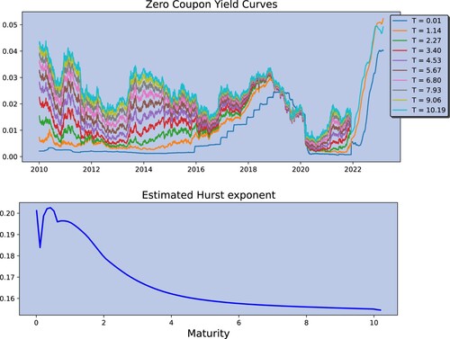Of course such a linear regression hinges on some assumptions in the form of $(r_t{)}_{t\ge 0}$ but a detailed analysis of short rate data is beyond the scope of the present paper, and we only provide here short insights into the potential roughness of short rates dynamics. We consider the sports interest rate data from Option Metrics.¹ We consider the data from 4/1/2010 until 28/2/2023. For different dates within this period, figure 1 shows the available data points (circles) as well as the interpolation by splines (the extrapolation is assumed flat). In figure 2, we compute the time series of the yield curves, for each (interpolated) maturities and estimate the Hurst exponent for each maturity.

Figure 1. Examples of rates curves over different days from the OptionMetrics rates data.

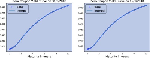
Figure 2. Top: Time series of the OptionMetrics rates for different maturities. Bottom: Estimation of the Hurst exponent for the OptionMetrics rates data.

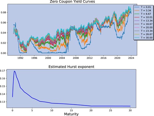
A similar analysis on the US Daily Treasury Par Yield Curve Rates² yields figure 3.

Figure 3. Top: Time series of the US Treasury rates for different maturities. Bottom: Estimation of the Hurst exponent for the US Treasury rates.

2. Gaussian martingale driver

2.1. Dynamics of the zero-coupon bond price

We assume first that $\mathfrak{W}$ is a continuous Gaussian martingale with ${\gamma }_{\mathfrak{W}}\left(t\right):=\mathbb{E}\left[{\mathfrak{W}}_t^2\right]$ finite for all $t\ge 0$. In this case, the (predictable) quadratic variation process ${\gamma }_{\mathfrak{W}}(\cdot )$ is clearly deterministic, but also continuous and increasing, and therefore its derivative ${\gamma }_{\mathfrak{W}}^{\prime }$ exists almost everywhere. In order to ensure existence of the rate process in (1(1) $\begin{array}{r}{r}_t=\theta \left(t\right)+{\int }_0^t\phi (t,u)\mathrm{d}{\mathfrak{W}}_u=\theta \left(t\right)+{\left(\phi \right(t,\cdot )\circ \mathfrak{W})}_t,\end{array}$(1) ), we assume the following (we write $\mathrm{d}\lambda$ for the Lebesgue measure on ${\mathbb{R}}_{+}$):

Assumption 2.1

For each $t\in [0,T]$, $\phi (t,\cdot )\in L^1\left(\mathrm{d}\lambda \right)\cap L^2\left({\gamma }_{\mathfrak{W}}\right)$, and φ is of convolution type (5(5) $\begin{array}{r}\phi (t,u)=\phi (t-u).\end{array}$(5) ).

Lemma 2.2

Under assumption 2.1, $\left({\mathrm{\Xi }}_T\right(t,\cdot )\circ \mathfrak{W}{)}_t$ is an $({\mathcal{F}}_t{)}_{t\in [0,T]}$ Gaussian semimartingale.

Proof.

From (2(2) $\begin{array}{r}{\mathrm{\Xi }}_T(t,u):=-{\int }_t^T\phi (s,u)\mathrm{d}s\text{ and}{\mathrm{\Xi }}_T\left(u\right):={\mathrm{\Xi }}_T(u,u)\end{array}$(2) ), ${\mathrm{\Xi }}_T$ is in general not in convolution form (5(5) $\begin{array}{r}\phi (t,u)=\phi (t-u).\end{array}$(5) ). However, since φ is, we can write $\begin{array}{rl}{\mathrm{\Xi }}_T(t,u)& :=-{\int }_t^T\phi (s,u)\mathrm{d}s=-{\int }_t^T\phi (s-u)\mathrm{d}s\\ & =\mathrm{\Phi }(T-u)-\mathrm{\Phi }(t-u),\end{array}$ where the function Φ is defined as $\mathrm{\Phi }\left(z\right):=-{\int }_{\cdot }^z\phi \left(u\right)\mathrm{d}u$. The stochastic integral then reads $\begin{array}{rl}{\left({\mathrm{\Xi }}_T\right(t,\cdot )\circ \mathfrak{W})}_t& ={\int }_0^t{\mathrm{\Xi }}_T(t,u)\mathrm{d}\\ {\mathfrak{W}}_u& =-{\int }_0^t\left[\mathrm{\Phi }\right(t-u)-\mathrm{\Phi }(T-u\left)\right]\mathrm{d}{\mathfrak{W}}_u,\end{array}$ which corresponds to a two-sided moving average process in the sense of Basse-O'Connor and Graversen (2010, Section 5.2). Assumption 2.1 then implies that for each $t\in [0,T]$, the function ${\mathrm{\Xi }}_T(t,\cdot )$ is absolutely continuous on $[0,t]$ and ${\mathrm{\partial }}_t{\mathrm{\Xi }}_T(t,\cdot )\in L^2\left({\gamma }_{\mathfrak{W}}\right)$ and the statement follows from Basse-O'Connor and Graversen (2010, Theorem 5.5).

Remark 2.3

• The $L^2$ property ensures that the stochastic integral $\left(\phi \right(t-\cdot )\circ \mathfrak{W}{)}_t$ is well defined.

• The assumption does not imply that the short rate itself, while Gaussian, is a semimartingale.

Proposition 2.4

The price of the zero-coupon bond at time t reads $\begin{array}{r}{P}_{t,T}=\exp \{-{\mathrm{\Theta }}_{t,T}+\frac{1}{2}{\int }_t^T{\mathrm{\Xi }}_T(u{)}^2\mathrm{d}u+{\left({\mathrm{\Xi }}_T\right(t,\cdot )\circ \mathfrak{W})}_t\},\end{array}$ and the discounted bond price ${\tilde{P}}_{t,T}:=P_{t,T}\exp \{-{\int }_0^t{r}_s\mathrm{d}s\}$ is a $\mathbb{Q}$-martingale satisfying $\begin{array}{r}\frac{\mathrm{d}{\tilde{P}}_{t,T}}{{\tilde{P}}_{t,T}}={\mathrm{\Xi }}_T\left(t\right)\mathrm{d}{\mathfrak{W}}_t.\end{array}$

Corollary 2.5

The instantaneous forward rate satisfies $f_{\mathrm{TT}}=r_T$ and, for all $t\in [0,T)$, $\begin{array}{r}{f}_{t,T}=\theta \left(T\right)+{\int }_0^t\phi (T,u)\mathrm{d}{\mathfrak{W}}_u+{\int }_t^T\phi (T,u){\mathrm{\Xi }}_T\left(u\right)\mathrm{d}u.\end{array}$

In differential form, for any fixed T>0, for $t\in [0,T]$, this is equivalent to $\begin{array}{r}\mathrm{d}{f}_{t,T}=\phi (T-t)\mathrm{d}{\mathfrak{W}}_t-\phi (T-t){\mathrm{\Xi }}_T\left(t\right)\mathrm{d}t.\end{array}$

Algorithm 2.6

For simulation purposes, we consider a time grid $\mathcal{T}:=\{0=t_0<t_1<\cdots <t_N=T\}$ and discretize the stochastic integral along this grid with left-point approximations as $\begin{array}{rl}& {\left({\mathrm{\Xi }}_T\right(t_i,\cdot )\circ \mathfrak{W})}_{t_i}\\ & ={\int }_0^{t_i}{\mathrm{\Xi }}_T(t_i,u)\mathrm{d}{\mathfrak{W}}_u\\ & \approx \sum _{k=0}^{i-1}{\mathrm{\Xi }}_T(t_i,t_k)({\mathfrak{W}}_{t_{k+1}}-{\mathfrak{W}}_{t_k}),\text{ for each }i=1,\dots ,N.\end{array}$ The vector $\left({\mathrm{\Xi }}_T\right(t_i,\cdot )\circ \mathfrak{W}{)}_{t_i\in \mathcal{T}}$ of stochastic integrals can then be simulated along the grid directly as $\begin{array}{rl}& \left(\begin{array}{c}{\left({\mathrm{\Xi }}_T\right(t_1,\cdot )\circ \mathfrak{W})}_{t_1}\\ ⋮\\ {\left({\mathrm{\Xi }}_T\right(t_N,\cdot )\circ \mathfrak{W})}_{t_N}\end{array}\right)\\ & \approx \left(\begin{array}{cccc}{\mathrm{\Xi }}_T(t_1,t_0)& & & \\ {\mathrm{\Xi }}_T(t_2,t_0)& {\mathrm{\Xi }}_T(t_2,t_1)& & \\ ⋮& \ddots & \ddots & \\ {\mathrm{\Xi }}_T(t_{N-1},t_0)& {\mathrm{\Xi }}_T(t_{N-1},t_1)& \dots & {\mathrm{\Xi }}_T(t_{N-1},t_{N-2})\\ {\mathrm{\Xi }}_T(t_N,t_0)& {\mathrm{\Xi }}_T(t_N,t_1)& \dots & {\mathrm{\Xi }}_T(t_N,t_{N-1})\end{array}\right)\\ & \times \left(\begin{array}{c}{\mathfrak{W}}_{t_1}-{\mathfrak{W}}_{t_0}\\ ⋮\\ {\mathfrak{W}}_{t_N}-{\mathfrak{W}}_{t_{N-1}}\end{array}\right),\end{array}$ where the middle matrix is lower triangular (we omit the null terms everywhere for clarity).

Example 2.7

With $\phi \left(t\right)=\sigma {\mathrm{e}}^{-\mathrm{\kappa t}}$, for $\sigma >0$, $\theta \left(t\right):=r_0{\mathrm{e}}^{-\mathrm{\kappa t}}+\mu (1-{\mathrm{e}}^{-\mathrm{\kappa t}})$ and $\mathfrak{W}=W$ a Brownian motion, we recover exactly the Vasicek model (Vasicek 1977), namely $r_t=r_0+\kappa {\int }_0^t(\mu -r_s)\mathrm{d}s+\sigma W_t$.

Example 2.8

Consider the extension of the Vasicek model proposed by Hull and White (1990), where $\mathrm{d}{r}_t=\left(\zeta \right(t)-a(t\left)r_t\right)\mathrm{d}t+\sigma \left(t\right)\mathrm{d}{W}_t,$ where $\zeta (\cdot ),a(\cdot )$ and $\sigma (\cdot )$ are sufficiently smooth deterministic functions of time. Direct computations yield the solution, with $A\left(t\right):={\int }_0^{t}a\left(s\right)\mathrm{d}s$, $\begin{array}{r}{r}_t=r_0+{\int }_0^t{\mathrm{e}}^{-\left(A\right(t)-A(s\left)\right)}\zeta \left(s\right)\mathrm{d}s+{\int }_0^t{\mathrm{e}}^{-\left(A\right(t)-A(s\left)\right)}\sigma \left(s\right)\mathrm{d}{W}_s.\end{array}$ Letting $\begin{array}{rl}\theta \left(t\right)& :=r_0+{\int }_0^t{\mathrm{e}}^{-\left(A\right(t)-A(s\left)\right)}\zeta \left(s\right)\mathrm{d}s,\\ \phi (t,s)& :={\mathrm{e}}^{-\left(A\right(t)-A(s\left)\right)}\text{ and}\mathrm{d}{\mathfrak{W}}_t=\sigma \left(t\right)\mathrm{d}{W}_t\end{array}$ makes it coincide exactly with our setup in (1(1) $\begin{array}{r}{r}_t=\theta \left(t\right)+{\int }_0^t\phi (t,u)\mathrm{d}{\mathfrak{W}}_u=\theta \left(t\right)+{\left(\phi \right(t,\cdot )\circ \mathfrak{W})}_t,\end{array}$(1) ). Now assumption 2.1 holds if and only if $A\left(t\right)-A\left(s\right)=A(t-s)$ for all $0\le s\le t$, namely when the function a is linear or constant. Note that, as mentioned in Brigo and Mercurio (2006, Section 3.3), the function a is often assumed constant in practice.

Proof of proposition 2.4.

The price of the zero-coupon bond at time t then reads (6) $\begin{array}{rl}& P_{t,T}:={\mathbb{E}}_t^{\mathbb{Q}}[\exp \{-{\int }_t^T{r}_s\mathrm{d}s\}]\\ & ={\mathbb{E}}_t^{\mathbb{Q}}[\exp \{-{\int }_t^T\left(\theta \right(s)+{\int }_0^s\phi (s,u\left)\mathrm{d}{\mathfrak{W}}_u\right)\mathrm{d}s\}]\\ & ={\mathrm{e}}^{-{\mathrm{\Theta }}_{t,T}}{\mathbb{E}}_t^{\mathbb{Q}}[\exp \{-{\int }_t^T\left({\int }_0^s\phi \right(s,u\left)\mathrm{d}{\mathfrak{W}}_u\right)\mathrm{d}s\}].\end{array}$(6) Using Fubini, we can write (7) $\begin{array}{rl}& -{\int }_t^T\left({\int }_0^s\phi \right(s,u\left)\mathrm{d}{\mathfrak{W}}_u\right)\mathrm{d}s\\ & =-{\int }_0^t\left({\int }_t^T\phi \right(s,u\left)\mathrm{d}s\right)\mathrm{d}{\mathfrak{W}}_u-{\int }_t^T\left({\int }_u^T\phi \right(s,u\left)\mathrm{d}s\right)\mathrm{d}{\mathfrak{W}}_u\\ & ={\int }_0^t{\mathrm{\Xi }}_T(t,u)\mathrm{d}{\mathfrak{W}}_u+{\int }_t^T{\mathrm{\Xi }}_T\left(u\right)\mathrm{d}{\mathfrak{W}}_u,\end{array}$(7) using (2(2) $\begin{array}{r}{\mathrm{\Xi }}_T(t,u):=-{\int }_t^T\phi (s,u)\mathrm{d}s\text{ and}{\mathrm{\Xi }}_T\left(u\right):={\mathrm{\Xi }}_T(u,u)\end{array}$(2) ). Plugging this into (6(6) $\begin{array}{rl}& P_{t,T}:={\mathbb{E}}_t^{\mathbb{Q}}[\exp \{-{\int }_t^T{r}_s\mathrm{d}s\}]\\ & ={\mathbb{E}}_t^{\mathbb{Q}}[\exp \{-{\int }_t^T\left(\theta \right(s)+{\int }_0^s\phi (s,u\left)\mathrm{d}{\mathfrak{W}}_u\right)\mathrm{d}s\}]\\ & ={\mathrm{e}}^{-{\mathrm{\Theta }}_{t,T}}{\mathbb{E}}_t^{\mathbb{Q}}[\exp \{-{\int }_t^T\left({\int }_0^s\phi \right(s,u\left)\mathrm{d}{\mathfrak{W}}_u\right)\mathrm{d}s\}].\end{array}$(6) ), the zero-coupon bond then reads $\begin{array}{rl}{P}_{t,T}& ={\mathrm{e}}^{-{\mathrm{\Theta }}_{t,T}}\exp \left\{{\int }_0^t{\mathrm{\Xi }}_T\right(t,u\left)\mathrm{d}{\mathfrak{W}}_u\right\}{\mathbb{E}}_t^{\mathbb{Q}}\\ & \times [\exp \left\{{\int }_t^T{\mathrm{\Xi }}_T\right(u\left)\mathrm{d}{\mathfrak{W}}_u\right\}]\\ & ={\mathrm{e}}^{-{\mathrm{\Theta }}_{t,T}}\exp \{{\left({\mathrm{\Xi }}_T\right(t,\cdot )\circ \mathfrak{W})}_t\}{\mathbb{E}}_t^{\mathbb{Q}}\left[{\mathrm{e}}^{{({\mathrm{\Xi }}_T\circ \mathfrak{W})}_{t,T}}\right].\end{array}$ Conditional on ${\mathcal{F}}_t$, $({\mathrm{\Xi }}_T\circ \mathfrak{W}{)}_{t,T}$ is centered Gaussian with ${\mathbb{V}}_t\left[\right({\mathrm{\Xi }}_T\circ \mathfrak{W}{)}_{t,T}]={\int }_t^T{\mathrm{\Xi }}_T(u{)}^2\mathrm{d}u$, hence $P_{t,T}={\mathrm{e}}^{-{\mathrm{\Theta }}_{t,T}}\exp \left\{\right({\mathrm{\Xi }}_T(t,\cdot )\circ \mathfrak{W}{)}_t+\frac{1}{2}{\int }_t^T{\mathrm{\Xi }}_T\left(u{)}^2\mathrm{d}u\right\}.$ By Fubini and assumption 2.1, $\begin{array}{rl}{\left({\mathrm{\Xi }}_T\right(t,\cdot )\circ \mathfrak{W})}_t& ={\int }_0^t{\mathrm{\Xi }}_T(t,u)\mathrm{d}{\mathfrak{W}}_u\\ & ={\int }_0^t\left({\mathrm{\Xi }}_T\right(u)+{\int }_u^t{\mathrm{\partial }}_s{\mathrm{\Xi }}_T(s,u\left)\mathrm{d}s\right)\mathrm{d}{\mathfrak{W}}_u\\ & ={\int }_0^t{\mathrm{\Xi }}_T\left(u\right)\mathrm{d}{\mathfrak{W}}_u+{\int }_0^t{\int }_u^t{\mathrm{\partial }}_s{\mathrm{\Xi }}_T(s,u)\mathrm{d}s\mathrm{d}{\mathfrak{W}}_u\\ & ={\int }_0^t{\mathrm{\Xi }}_T\left(u\right)\mathrm{d}{\mathfrak{W}}_u+{\int }_0^t{\int }_0^s{\mathrm{\partial }}_s{\mathrm{\Xi }}_T(s,u)\mathrm{d}{\mathfrak{W}}_u\mathrm{d}s\\ & ={\int }_0^t{\mathrm{\Xi }}_T\left(u\right)\mathrm{d}{\mathfrak{W}}_u+{\int }_0^t{\int }_0^s\phi (s,u)\mathrm{d}{\mathfrak{W}}_u\mathrm{d}s.\end{array}$ This is an $L^1$-Dirichlet process (Russo and Tudor 2006, Definition 2), written as a decomposition of a local martingale and a term with zero quadratic variation. Therefore $〈\log \left(P_{\cdot ,T}\right),\log \left(P_{\cdot ,T}\right){〉}_t={\int }_0^t{\mathrm{\Xi }}_T(u{)}^2\mathrm{d}u$ and (8) $\begin{array}{rl}\mathrm{d}\log \left(P_{\cdot ,T}\right)& =\left(\theta \right(t)+{\left({\mathrm{\partial }}_t{\mathrm{\Xi }}_T\right(t,\cdot )\circ \mathfrak{W})}_t-\frac{1}{2}{\mathrm{\Xi }}_T(t{)}^2)\mathrm{d}t\\ & +{\mathrm{\Xi }}_T\left(t\right)\mathrm{d}{\mathfrak{W}}_t.\end{array}$(8) Now, Itô's formula with $X_t:=\log \left(P_{t,T}\right)$, using (8(8) $\begin{array}{rl}\mathrm{d}\log \left(P_{\cdot ,T}\right)& =\left(\theta \right(t)+{\left({\mathrm{\partial }}_t{\mathrm{\Xi }}_T\right(t,\cdot )\circ \mathfrak{W})}_t-\frac{1}{2}{\mathrm{\Xi }}_T(t{)}^2)\mathrm{d}t\\ & +{\mathrm{\Xi }}_T\left(t\right)\mathrm{d}{\mathfrak{W}}_t.\end{array}$(8) ) yields $P_{T,T}=P_{t,T}+{\int }_t^T{P}_{s,T}\mathrm{d}{X}_s+\frac{1}{2}{\int }_t^T{P}_{s,T}\mathrm{d}〈X,X{〉}_s$, hence, for each T>0, $\mathrm{d}{P}_{T,T}=\mathrm{d}{P}_{t,T}-P_{t,T}\mathrm{d}{X}_t-\frac{1}{2}{P}_{t,T}\mathrm{d}〈X,X{〉}_t$, and therefore, since $P_{T,T}=1$, $\begin{array}{rl}\frac{\mathrm{d}{P}_{t,T}}{P_{t,T}}& =\mathrm{d}{X}_t+\frac{1}{2}\mathrm{d}〈X,X{〉}_t\\ & =(\underset{r_t}{\underbrace{\theta \left(t\right)+{\left({\mathrm{\partial }}_t{\mathrm{\Xi }}_T\right(t,\cdot )\circ \mathfrak{W})}_t}}-\frac{1}{2}{\mathrm{\Xi }}_T(t{)}^2)\mathrm{d}t\\ & +{\mathrm{\Xi }}_T\left(t\right)\mathrm{d}{\mathfrak{W}}_t+\frac{1}{2}\mathrm{d}\left({\int }_0^t{\mathrm{\Xi }}_T\right(u{)}^2\mathrm{d}u)\\ & =r_t\mathrm{d}t+{\mathrm{\Xi }}_T\left(t\right)\mathrm{d}{\mathfrak{W}}_t-\frac{1}{2}{\mathrm{\Xi }}_T(t{)}^2\mathrm{d}t\\ & +\frac{1}{2}{\mathrm{\Xi }}_T(t{)}^2\mathrm{d}t=r_t\mathrm{d}t+{\mathrm{\Xi }}_T(t)\mathrm{d}{\mathfrak{W}}_t.\end{array}$ The dynamics of the discounted zero-coupon bond price in the lemma follows immediately.

Proof of corollary 2.5.

It follows by direct computation starting from the instantaneous forward rate (4(4) $\begin{array}{r}{f}_{t,T}:=-{\mathrm{\partial }}_T\log P_{t,T}.\end{array}$(4) ): $\begin{array}{rl}{f}_{t,T}& ={\mathrm{\partial }}_T{\mathrm{\Theta }}_{t,T}-{\mathrm{\partial }}_T{\int }_0^t{\mathrm{\Xi }}_T(t,u)\mathrm{d}{\mathfrak{W}}_u-\frac{1}{2}{\mathrm{\partial }}_T{\int }_t^T{\mathrm{\Xi }}_T(u{)}^2\mathrm{d}u\\ & ={\mathrm{\partial }}_T{\mathrm{\Theta }}_{t,T}-{\mathrm{\partial }}_T{\int }_0^t(-{\int }_t^T\phi (s,u\left)\mathrm{d}s\right)\mathrm{d}{\mathfrak{W}}_u\\ & -\frac{1}{2}{\mathrm{\partial }}_T{\int }_t^T{(-{\int }_u^T\phi (s,u\left)\mathrm{d}s\right)}^2\mathrm{d}u\\ & =\theta \left(T\right)+{\int }_0^t{\mathrm{\partial }}_T\left({\int }_t^T\phi \right(s,u\left)\mathrm{d}s\right)\mathrm{d}{\mathfrak{W}}_u\\ & -\frac{1}{2}{\mathrm{\partial }}_T{\int }_t^T{\left({\int }_u^T\phi \right(s,u\left)\mathrm{d}s\right)}^2\mathrm{d}u\\ & =\theta \left(T\right)+{\int }_0^t\phi (T,u)\mathrm{d}{\mathfrak{W}}_u\\ & -\frac{1}{2}\left({\int }_T^T\phi \right(s,T{)}^2\mathrm{d}s+{\int }_t^T{\mathrm{\partial }}_T\left[{\left({\int }_u^T\phi \right(s,u\left)\mathrm{d}s\right)}^2\right]\mathrm{d}u)\\ & =\theta \left(T\right)+{\int }_0^t\phi (T,u)\mathrm{d}{\mathfrak{W}}_u\\ & -{\int }_t^T\phi (T,u)\left({\int }_u^T\phi \right(s,u\left)\mathrm{d}s\right)\mathrm{d}u\\ & =\theta \left(T\right)+{\int }_0^t\phi (T,u)\mathrm{d}{\mathfrak{W}}_u+{\int }_t^T\phi (T,u){\mathrm{\Xi }}_T\left(u\right)\mathrm{d}u.\end{array}$

Remark 2.9

The two lemmas above correspond to the two sides of the Heath–Jarrow–Morton framework. From the expression of the instantaneous forward rate, let ${\alpha }_{t,T}:=\phi (T-t){\mathrm{\Xi }}_T\left(t\right)$ and ${\text{β}}_{t,T}:=\phi (T-t)$, so that $\mathrm{d}{f}_{t,T}={\text{β}}_{t,T}\mathrm{d}{\mathfrak{W}}_t-{\alpha }_{t,T}\mathrm{d}t$, and consider the discounted bond price $\begin{array}{rl}{\tilde{P}}_{t,T}& :=P_{t,T}\exp \{-{\int }_0^t{r}_s\mathrm{d}s\}\\ & =\exp \{-{\int }_0^t{r}_s\mathrm{d}s-{\int }_t^T{f}_{t,s}\mathrm{d}s\}=:\exp \left\{Z_t\right\}.\end{array}$ Itôs' formula then yields (9) $\begin{array}{r}\frac{\mathrm{d}{\tilde{P}}_{t,T}}{{\tilde{P}}_{t,T}}=\mathrm{d}{Z}_t+\frac{1}{2}\mathrm{d}〈Z,Z{〉}_t.\end{array}$(9) From the differential form of $f_{t,T}$, we can write, for any $t\in [0,T)$, $\begin{array}{rl}{f}_{t,T}& =f_{0,T}+{\int }_0^t\mathrm{d}{f}_{s,T}=f_{0,T}\\ & +{\int }_0^t(\phi (T,u)\mathrm{d}{\mathfrak{W}}_u-\phi (T,u){\mathrm{\Xi }}_T\left(u\right)\mathrm{d}u)\\ & =f_{0,T}+{\int }_0^t{\text{β}}_{u,T}\mathrm{d}{\mathfrak{W}}_u+{\int }_0^t{\alpha }_{u,T}\mathrm{d}u,\end{array}$ so that, using stochastic Fubini, we obtain $\begin{array}{rl}{F}_{t,T}& :={\int }_t^T{f}_{t,s}\mathrm{d}s={\int }_t^T(f_{0,s}+{\int }_0^t{\text{β}}_{u,s}\mathrm{d}{\mathfrak{W}}_u+{\int }_0^t{\alpha }_{u,s}\mathrm{d}u)\mathrm{d}s\\ & ={\int }_t^T{f}_{0,s}\mathrm{d}s+{\int }_0^t{\int }_t^T{\text{β}}_{u,s}\mathrm{d}s\mathrm{d}{\mathfrak{W}}_u+{\int }_0^t{\int }_t^T{\alpha }_{u,s}\mathrm{d}s\mathrm{d}u.\end{array}$ Now, $\begin{array}{rl}{\int }_t^T{f}_{0,s}\mathrm{d}s& ={\int }_t^T(f_{s,s}-{\int }_0^s{\mathrm{\partial }}_u{f}_{u,s}\mathrm{d}u)\mathrm{d}s\\ & ={\int }_t^T{r}_s\mathrm{d}s-{\int }_0^t{\int }_t^T{\mathrm{\partial }}_u{f}_{u,s}\mathrm{d}s\mathrm{d}u\\ & -{\int }_t^T{\int }_u^T{\mathrm{\partial }}_u{f}_{u,s}\mathrm{d}s\mathrm{d}u\\ & ={\int }_t^T{r}_s\mathrm{d}s-{\int }_0^t({\int }_t^T{\mathrm{\partial }}_u{f}_{u,s}\mathrm{d}s-{\int }_u^T{\mathrm{\partial }}_u{f}_{u,s}\mathrm{d}s)\mathrm{d}u\\ & -{\int }_0^T{\int }_u^T{\mathrm{\partial }}_u{f}_{u,s}\mathrm{d}s\mathrm{d}u\\ & ={\int }_t^T{r}_s\mathrm{d}s+{\int }_0^t{\int }_u^t{\mathrm{\partial }}_u{f}_{u,s}\mathrm{d}s\mathrm{d}u\\ & -{\int }_0^T{\int }_u^T{\mathrm{\partial }}_u{f}_{u,s}\mathrm{d}s\mathrm{d}u,\end{array}$ using Fubini, so that $\begin{array}{rl}{F}_{t,T}& =\underset{{\int }_t^T{f}_{0,s}\mathrm{d}s}{\underbrace{{\int }_t^T{r}_s\mathrm{d}s+{\int }_0^t{\int }_u^t{\mathrm{\partial }}_u{f}_{u,s}\mathrm{d}s\mathrm{d}u-{\int }_0^T{\int }_u^T{\mathrm{\partial }}_u{f}_{u,s}\mathrm{d}s\mathrm{d}u}}\\ & +{\int }_0^t{\int }_t^T{\text{β}}_{u,s}\mathrm{d}s\mathrm{d}{\mathfrak{W}}_u+{\int }_0^t{\int }_t^T{\alpha }_{u,s}\mathrm{d}s\mathrm{d}u,\end{array}$ and $\mathrm{d}{F}_{t,T}=({\int }_t^T{\alpha }_{t,s}\mathrm{d}s-r_t)\mathrm{d}t+\left({\int }_t^T{\text{β}}_{t,s}\mathrm{d}s\right)\mathrm{d}{\mathfrak{W}}_t$. Therefore, $\begin{array}{rl}\mathrm{d}{Z}_t& =\mathrm{d}(-{\int }_0^t{r}_s\mathrm{d}s-{\int }_t^T{f}_{t,s}\mathrm{d}s)=-r_t\mathrm{d}t\\ & -\mathrm{d}{F}_{t,T}=-r_t\mathrm{d}t\\ & -\mathrm{d}{F}_{t,T}\\ & =-\left({\int }_t^T{\alpha }_{t,s}\mathrm{d}s\right)\mathrm{d}t-\left({\int }_t^T{\text{β}}_{t,s}\mathrm{d}s\right)\mathrm{d}{\mathfrak{W}}_t,\end{array}$ and (9(9) $\begin{array}{r}\frac{\mathrm{d}{\tilde{P}}_{t,T}}{{\tilde{P}}_{t,T}}=\mathrm{d}{Z}_t+\frac{1}{2}\mathrm{d}〈Z,Z{〉}_t.\end{array}$(9) ) gives $\begin{array}{rl}\frac{\mathrm{d}{\tilde{P}}_{t,T}}{{\tilde{P}}_{t,T}}& =-({\int }_t^T{\alpha }_{t,s}\mathrm{d}s-\frac{1}{2}{\left({\int }_t^T{\text{β}}_{t,s}\mathrm{d}s\right)}^2)\mathrm{d}t\\ & -\left({\int }_t^T{\text{β}}_{t,s}\mathrm{d}s\right)\mathrm{d}{\mathfrak{W}}_t.\end{array}$ The discounted process $({\tilde{P}}_{t,T}{)}_{t\in [0,T]}$ is a local martingale if and only if its drift is null: for $t\in (0,T)$, $\begin{array}{rl}& {\mathrm{\partial }}_T\{{\int }_t^T{\alpha }_{t,s}\mathrm{d}s-\frac{1}{2}{\left[{\int }_t^T{\text{β}}_{t,s}\mathrm{d}s\right]}^2\}\\ & ={\alpha }_{t,T}-{\text{β}}_{t,T}{\int }_t^T{\text{β}}_{t,s}\mathrm{d}s=\phi (T-t)\\ & \times \left[{\mathrm{\Xi }}_T\right(t)-{\int }_t^T\phi (s,t\left)\mathrm{d}s\right],\end{array}$ which is equal to zero by definition of the functions. Therefore the drift (as a function of T) is constant. Since it is trivially equal to zero at T = t, it is null everywhere and $({\tilde{P}}_{t,T}{)}_{t\in [0,T]}$ is a $\mathbb{Q}$-local martingale.

2.2. Convexity adjustments

We now enter the core of the paper, investigating the influence of the Gaussian driver on the convexity of bond prices. We first start with the following simple proposition:

Proposition 2.10

For any $T,\tau \ge 0$, $\begin{array}{rl}\mathrm{d}\left(\frac{1}{P_{t,\tau }}\right)& =\frac{\left({\mathrm{\Xi }}_{\tau }\right(t,t{)}^2{\gamma }_{\mathfrak{W}}^{\prime }\left(t\right)-r_t)\mathrm{d}t}{P_{t,\tau }}-\frac{{\mathrm{\Xi }}_{\tau }(t,t)}{P_{t,\tau }}\mathrm{d}{\mathfrak{W}}_t,\\ \mathrm{d}\left(\frac{P_{t,T}}{P_{t,\tau }}\right)& =\frac{P_{t,T}}{P_{t,\tau }}({\mathrm{\Xi }}_T(t,t)-{\mathrm{\Xi }}_{\tau }(t,t))\\ & \times \{-{\mathrm{\Xi }}_{\tau }(t,t){\gamma }_{\mathfrak{W}}^{\prime }\left(t\right)\mathrm{d}t+\mathrm{d}{\mathfrak{W}}_t\},\end{array}$ and there exists a probability measure ${\mathbb{Q}}^{\tau }$ such that ${\mathfrak{W}}_t^{{\mathbb{Q}}^{\tau }}$ is a ${\mathbb{Q}}^{\tau }$-Gaussian martingale and (10) $\begin{array}{r}\mathrm{d}\left(\frac{P_{t,T}}{P_{t,\tau }}\right)=\frac{P_{t,T}}{P_{t,\tau }}{\mathrm{\Sigma }}_t^{T,\tau }\mathrm{d}{\mathfrak{W}}_t^{{\mathbb{Q}}^{\tau }},\end{array}$(10) under ${\mathbb{Q}}^{\tau }$, where ${\mathrm{\Sigma }}_t^{T,\tau }:={\mathrm{\Xi }}_T\left(t\right)-{\mathrm{\Xi }}_{\tau }\left(t\right)=\mathrm{\Phi }(T-t)-\mathrm{\Phi }(\tau -t)$.

Note that, from the definition of ${\mathrm{\Xi }}_T$ in (2(2) $\begin{array}{r}{\mathrm{\Xi }}_T(t,u):=-{\int }_t^T\phi (s,u)\mathrm{d}s\text{ and}{\mathrm{\Xi }}_T\left(u\right):={\mathrm{\Xi }}_T(u,u)\end{array}$(2) ), ${\mathrm{\Sigma }}_t^{T,\tau }$ is non-negative whenever $\tau \ge T$. In standard Fixed Income literature, the probability measure ${\mathbb{Q}}^{\tau }$ corresponds to the τ-forward measure.

Proof.

From the definition of the zero-coupon price (3(3) $\begin{array}{r}{P}_{t,T}:={\mathbb{E}}_t^{\mathbb{Q}}\left[B_{t,T}\right],\text{ where}{B}_{t,T}:=\exp \{-{\int }_t^T{r}_s\mathrm{d}s\},\end{array}$(3) ) and proposition 2.4, $P_{t,T}>0$ is strictly positive almost surely and $\begin{array}{r}\frac{\mathrm{d}{P}_{t,T}}{P_{t,T}}=r_t\mathrm{d}t+{\mathrm{\Xi }}_T(t,t)\mathrm{d}{\mathfrak{W}}_t,\end{array}$ and therefore Itô's formula implies that, for any $0\le t\le \tau$, $\begin{array}{rl}\mathrm{d}\left(\frac{1}{P_{t,\tau }}\right)& =-\frac{\mathrm{d}{P}_{t,\tau }}{P_{t,\tau }^2}+\frac{\mathrm{d}〈P_{t,\tau },P_{t,\tau }〉}{P_{t,\tau }^3}\\ & =\frac{({\mathrm{\Xi }}_{\tau }(t,t{)}^2{\gamma }_{\mathfrak{W}}^{\prime }(t)-r_t)\mathrm{d}t}{P_{t,\tau }}-\frac{{\mathrm{\Xi }}_{\tau }(t,t)\mathrm{d}{\mathfrak{W}}_t}{P_{t,\tau }}.\end{array}$ Therefore $\begin{array}{rl}\mathrm{d}\left(\frac{P_{t,T}}{P_{t,\tau }}\right)& =P_{t,T}\mathrm{d}\left(\frac{1}{P_{t,\tau }}\right)+\frac{\mathrm{d}{P}_{t,T}}{P_{t,\tau }}+\mathrm{d}{P}_{t,T}\cdot \mathrm{d}\left(\frac{1}{P_{t,\tau }}\right)\\ & =\frac{P_{t,T}}{P_{t,\tau }}\left\{({\mathrm{\Xi }}_{\tau }\right(t,t{)}^2{\gamma }_{\mathfrak{W}}^{\prime }\left(t\right)-r_t)\mathrm{d}t\\ & -{\mathrm{\Xi }}_{\tau }(t,t)\mathrm{d}{\mathfrak{W}}_t+(r_t\mathrm{d}t+{\mathrm{\Xi }}_T(t,t)\mathrm{d}{\mathfrak{W}}_t)\\ & -{\mathrm{\Xi }}_T(t,t){\mathrm{\Xi }}_{\tau }(t,t){\gamma }_{\mathfrak{W}}^{\prime }\left(t\right)\mathrm{d}t\}\\ & =\frac{P_{t,T}}{P_{t,\tau }}({\mathrm{\Xi }}_T(t,t)-{\mathrm{\Xi }}_{\tau }(t,t))\\ & \times \{-{\mathrm{\Xi }}_{\tau }(t,t){\gamma }_{\mathfrak{W}}^{\prime }\left(t\right)\mathrm{d}t+\mathrm{d}{\mathfrak{W}}_t\}.\end{array}$ Define now the Doléans–Dade exponential $\begin{array}{rl}{M}_t& :=\exp \left\{{\int }_0^t{\mathrm{\Xi }}_{\tau }\right(s,s\left){\gamma }_{\mathfrak{W}}^{\prime }\right(s)\mathrm{d}{\mathfrak{W}}_s\\ & -\frac{1}{2}{\int }_0^t{\left[{\mathrm{\Xi }}_{\tau }\right(s,s\left){\gamma }_{\mathfrak{W}}^{\prime }\right(s\left)\right]}^2\mathrm{d}s\},\end{array}$ and the Radon–Nikodym derivative $\frac{\mathrm{d}{\mathbb{Q}}^{\tau }}{\mathrm{d}\mathbb{P}}:=M$. Girsanov's Theorem (Øksendal 2003, Theorem 8.6.4) implies that ${\mathfrak{W}}_t^{{\mathbb{Q}}^{\tau }}:={\mathfrak{W}}_t-{\int }_0^t{\mathrm{\Xi }}_{\tau }(s,s){\gamma }_{\mathfrak{W}}^{\prime }\left(s\right)\mathrm{d}s$ is a Gaussian martingale and $\frac{P_{t,T}}{P_{t,\tau }}$ satisfies (10(10) $\begin{array}{r}\mathrm{d}\left(\frac{P_{t,T}}{P_{t,\tau }}\right)=\frac{P_{t,T}}{P_{t,\tau }}{\mathrm{\Sigma }}_t^{T,\tau }\mathrm{d}{\mathfrak{W}}_t^{{\mathbb{Q}}^{\tau }},\end{array}$(10) ) under ${\mathbb{Q}}^{\tau }$.

The following proposition is key and provides a closed-form expression for the convexity adjustments:

Proposition 2.11

For any $\tau \ge 0$ let ${\mathfrak{t}}_1,{\mathfrak{t}}_2\ge 0$. We then have $\begin{array}{r}{\mathbb{E}}^{{\mathbb{Q}}^{\tau }}\left[\frac{P_{t,{\mathfrak{t}}_1}}{P_{t,{\mathfrak{t}}_2}}\right]=\frac{P_{0,{\mathfrak{t}}_1}}{P_{0,{\mathfrak{t}}_2}}{\mathfrak{C}}_t^{\tau }({\mathfrak{t}}_1,{\mathfrak{t}}_2),\text{ for any }t\in [0,{\mathfrak{t}}_1\wedge {\mathfrak{t}}_2],\end{array}$ where ${\mathfrak{C}}_t^{\tau }({\mathfrak{t}}_1,{\mathfrak{t}}_2):=\exp \left\{{\int }_0^t\right({\mathrm{\Sigma }}_s^{{\mathfrak{t}}_2,\tau }-{\mathrm{\Sigma }}_s^{{\mathfrak{t}}_1,\tau }\left){\mathrm{\Sigma }}_s^{{\mathfrak{t}}_2,\tau }{\gamma }_{\mathfrak{W}}^{\prime }\right(s\left)\mathrm{d}s\right\}$ is the convexity adjustment factor.

Remark 2.12

• When t = 0 or ${\mathfrak{t}}_1={\mathfrak{t}}_2$ or $\frac{P_{t,{\mathfrak{t}}_1}}{P_{t,{\mathfrak{t}}_2}}$ is constant, there is no convexity adjustment, i.e. ${\mathfrak{C}}_t^{\tau }({\mathfrak{t}}_1,{\mathfrak{t}}_2)=1$.

• More interestingly, if ${\mathfrak{t}}_2=\tau$, then ${\mathrm{\Sigma }}_t^{{\mathfrak{t}}_2,\tau }={\mathrm{\Sigma }}_t^{{\mathfrak{t}}_2,{\mathfrak{t}}_2}={\mathrm{\Xi }}_{{\mathfrak{t}}_2}(t,t)-{\mathrm{\Xi }}_{{\mathfrak{t}}_2}(t,t)=0$ and $\begin{array}{rl}& {\mathfrak{C}}_t^{\tau }({\mathfrak{t}}_1,{\mathfrak{t}}_2)\\ & ={\mathfrak{C}}_t^{{\mathfrak{t}}_2}({\mathfrak{t}}_1,{\mathfrak{t}}_2)\\ & =\exp \left\{{\int }_0^t({\mathrm{\Sigma }}_s^{{\mathfrak{t}}_2,{\mathfrak{t}}_2}-{\mathrm{\Sigma }}_s^{{\mathfrak{t}}_1,{\mathfrak{t}}_2}){\mathrm{\Sigma }}_s^{{\mathfrak{t}}_2,{\mathfrak{t}}_2}{\gamma }_{\mathfrak{W}}^{\prime }\right(s\left)\mathrm{d}s\right\}=1,\end{array}$ and the process $(\frac{P_{t,{\mathfrak{t}}_1}}{P_{t,{\mathfrak{t}}_2}}{)}_{t\ge 0}$ is a ${\mathbb{Q}}^{\tau }$-martingale on $[0,{\mathfrak{t}}_1\wedge {\mathfrak{t}}_2]$.

• Regarding the sign of the convexity adjustment, we have $\begin{array}{rl}{\mathrm{\Sigma }}_s^{{\mathfrak{t}}_2,\tau }-{\mathrm{\Sigma }}_s^{{\mathfrak{t}}_1,\tau }& =({\mathrm{\Xi }}_{{\mathfrak{t}}_2}(s,s)-{\mathrm{\Xi }}_{\tau }(s,s))\\ & -({\mathrm{\Xi }}_{{\mathfrak{t}}_1}(s,s)-{\mathrm{\Xi }}_{\tau }(s,s))\\ & ={\mathrm{\Xi }}_{{\mathfrak{t}}_2}(s,s)-{\mathrm{\Xi }}_{{\mathfrak{t}}_1}(s,s)\\ & =-{\int }_s^{{\mathfrak{t}}_2}\phi (z,s)\mathrm{d}z+{\int }_s^{{\mathfrak{t}}_2}\phi (z,s)\mathrm{d}z\\ & =-{\int }_{{\mathfrak{t}}_1}^{{\mathfrak{t}}_2}\phi (z,s)\mathrm{d}z.\end{array}$ Since $\phi (\cdot )$ is strictly positive, then $\mathrm{sgn}({\mathrm{\Sigma }}_s^{{\mathfrak{t}}_2,\tau }-{\mathrm{\Sigma }}_s^{{\mathfrak{t}}_1,\tau })=\mathrm{sgn}({\mathfrak{t}}_1-{\mathfrak{t}}_2)$. Furthermore, since $\begin{array}{rl}{\mathrm{\Sigma }}_s^{{\mathfrak{t}}_2,\tau }& ={\mathrm{\Xi }}_{{\mathfrak{t}}_2}(s,s)-{\mathrm{\Xi }}_{\tau }(s,s)\\ & =-{\int }_s^{{\mathfrak{t}}_2}\phi (z,s)\mathrm{d}z+{\int }_s^{\tau }\phi (z,s)\mathrm{d}z\\ & ={\int }_{{\mathfrak{t}}_2}^{\tau }\phi (z,s)\mathrm{d}z,\end{array}$ then $\mathrm{sgn}\left({\mathrm{\Sigma }}_s^{{\mathfrak{t}}_2,\tau }\right)=\mathrm{sgn}(\tau -{\mathfrak{t}}_2)$, and therefore, assuming ${\gamma }_{\mathfrak{W}}^{\prime }$ strictly positive (as will be the case in all the examples considered here),

  Table 1. aaaa

  $\mathrm{sgn}(\log {\mathfrak{C}}_t^{\tau }({\mathfrak{t}}_1,{\mathfrak{t}}_2\left)\right)$	${\mathfrak{t}}_1>{\mathfrak{t}}_2$	${\mathfrak{t}}_1<{\mathfrak{t}}_2$
  $\tau <{\mathfrak{t}}_2$	negative	positive
  $\tau >{\mathfrak{t}}_2$	positive	negative

  Considering without generality ${\mathfrak{t}}_1<{\mathfrak{t}}_2$, the convexity adjustment is therefore greater than 1 for $\tau <{\mathfrak{t}}_2$ and less than 1 above.

Proof of proposition 2.11.

Under ${\mathbb{Q}}^{\tau }$, the process defined as $X_t:=P_{t,T}/P_{t,\tau }$ satisfies $\mathrm{d}{X}_t=X_t{\mathrm{\Sigma }}_t^{T,\tau }\mathrm{d}{\mathfrak{W}}_t^{{\mathbb{Q}}^{\tau }}$, is clearly lognormal and hence Itô's formula implies $\begin{array}{rl}\mathrm{d}\log \left(X_t\right)& =\frac{\mathrm{d}{X}_t}{X_t}-\frac{1}{2}\frac{\mathrm{d}〈X,X{〉}_t}{X_t^2}\\ & ={\mathrm{\Sigma }}_t^{T,\tau }\mathrm{d}{\mathfrak{W}}_t^{{\mathbb{Q}}^{\tau }}-\frac{1}{2}{\left({\mathrm{\Sigma }}_t^{T,\tau }\right)}^2{\gamma }_{\mathfrak{W}}^{\prime }\left(t\right)\mathrm{d}t,\end{array}$ so that $\begin{array}{r}{X}_t=X_0\exp \{{\int }_0^t{\mathrm{\Sigma }}_s^{T,\tau }\mathrm{d}{\mathfrak{W}}_s-\frac{1}{2}{\int }_0^t{\left({\mathrm{\Sigma }}_s^{T,\tau }\right)}^2{\gamma }_{\mathfrak{W}}^{\prime }(s\left)\mathrm{d}s\right\},\end{array}$ and therefore $\begin{array}{r}\frac{P_{t,T}}{P_{t,\tau }}=\frac{P_{0,T}}{P_{0,\tau }}\exp \{{\int }_0^t{\mathrm{\Sigma }}_s^{T,\tau }\mathrm{d}{\mathfrak{W}}_s-\frac{1}{2}{\int }_0^t{\left({\mathrm{\Sigma }}_s^{T,\tau }\right)}^2{\gamma }_{\mathfrak{W}}^{\prime }(s\left)\mathrm{d}s\right\}.\end{array}$ With successively $T={\mathfrak{t}}_1$ and $T={\mathfrak{t}}_2$, we can then write $\begin{array}{rl}\frac{P_{t,{\mathfrak{t}}_1}}{P_{t,\tau }}& =\frac{P_{0,{\mathfrak{t}}_1}}{P_{0,\tau }}\exp \{{\int }_0^t{\mathrm{\Sigma }}_s^{{\mathfrak{t}}_1,\tau }\mathrm{d}{\mathfrak{W}}_s-\frac{1}{2}{\int }_0^t{\left({\mathrm{\Sigma }}_s^{{\mathfrak{t}}_1,\tau }\right)}^2{\gamma }_{\mathfrak{W}}^{\prime }(s\left)\mathrm{d}s\right\},\\ \frac{P_{t,{\mathfrak{t}}_2}}{P_{t,\tau }}& =\frac{P_{0,{\mathfrak{t}}_2}}{P_{0,\tau }}\exp \{{\int }_0^t{\mathrm{\Sigma }}_s^{{\mathfrak{t}}_2,\tau }\mathrm{d}{\mathfrak{W}}_s-\frac{1}{2}{\int }_0^t{\left({\mathrm{\Sigma }}_s^{{\mathfrak{t}}_2,\tau }\right)}^2{\gamma }_{\mathfrak{W}}^{\prime }(s\left)\mathrm{d}s\right\},\end{array}$ so that $\begin{array}{rl}\frac{P_{t,{\mathfrak{t}}_1}}{P_{t,{\mathfrak{t}}_2}}& =\frac{P_{0,{\mathfrak{t}}_1}}{P_{0,{\mathfrak{t}}_2}}\exp \{{\int }_0^t{\mathrm{\Sigma }}_s^{{\mathfrak{t}}_1,\tau }\mathrm{d}{\mathfrak{W}}_s-\frac{1}{2}{\int }_0^t{\left({\mathrm{\Sigma }}_s^{{\mathfrak{t}}_1,\tau }\right)}^2{\gamma }_{\mathfrak{W}}^{\prime }(s)\mathrm{d}s\\ & -{\int }_0^t{\mathrm{\Sigma }}_s^{{\mathfrak{t}}_2,\tau }\mathrm{d}{\mathfrak{W}}_s+\frac{1}{2}{\int }_0^t{\left({\mathrm{\Sigma }}_s^{{\mathfrak{t}}_2,\tau }\right)}^2{\gamma }_{\mathfrak{W}}^{\prime }\left(s\right)\mathrm{d}s\}\\ & =\frac{P_{0,{\mathfrak{t}}_1}}{P_{0,{\mathfrak{t}}_2}}\exp \{{\int }_0^t({\mathrm{\Sigma }}_s^{{\mathfrak{t}}_1,\tau }-{\mathrm{\Sigma }}_s^{{\mathfrak{t}}_2,\tau })\mathrm{d}{\mathfrak{W}}_s\\ & +\frac{1}{2}{\int }_0^t[{\left({\mathrm{\Sigma }}_s^{{\mathfrak{t}}_2,\tau }\right)}^2-{\left({\mathrm{\Sigma }}_s^{{\mathfrak{t}}_1,\tau }\right)}^2]{\gamma }_{\mathfrak{W}}^{\prime }\left(s\right)\mathrm{d}s\}\\ & =\frac{P_{0,{\mathfrak{t}}_1}}{P_{0,{\mathfrak{t}}_2}}\exp \{{\int }_0^t({\mathrm{\Sigma }}_s^{{\mathfrak{t}}_1,\tau }-{\mathrm{\Sigma }}_s^{{\mathfrak{t}}_2,\tau })\mathrm{d}{\mathfrak{W}}_s\\ & +\frac{1}{2}{\int }_0^t{({\mathrm{\Sigma }}_s^{{\mathfrak{t}}_1,\tau }-{\mathrm{\Sigma }}_s^{{\mathfrak{t}}_2,\tau })}^2{\gamma }_{\mathfrak{W}}^{\prime }\left(s\right)\mathrm{d}s\}\\ & \exp \{\frac{1}{2}{\int }_0^t[{\left({\mathrm{\Sigma }}_s^{{\mathfrak{t}}_1,\tau }\right)}^2+{\left({\mathrm{\Sigma }}_s^{{\mathfrak{t}}_2,\tau }\right)}^2\\ & -2{\mathrm{\Sigma }}_s^{{\mathfrak{t}}_1,\tau }{\mathrm{\Sigma }}_s^{{\mathfrak{t}}_2,\tau }]{\gamma }_{\mathfrak{W}}^{\prime }\left(s\right)\mathrm{d}s\\ & +\frac{1}{2}{\int }_0^t[{\left({\mathrm{\Sigma }}_s^{{\mathfrak{t}}_2,\tau }\right)}^2-{\left({\mathrm{\Sigma }}_s^{{\mathfrak{t}}_1,\tau }\right)}^2]{\gamma }_{\mathfrak{W}}^{\prime }\left(s\right)\mathrm{d}s\}\\ & =\frac{P_{0,{\mathfrak{t}}_1}}{P_{0,{\mathfrak{t}}_2}}\exp \{{\int }_0^t({\mathrm{\Sigma }}_s^{{\mathfrak{t}}_1,\tau }-{\mathrm{\Sigma }}_s^{{\mathfrak{t}}_2,\tau })\mathrm{d}{\mathfrak{W}}_s\\ & +\frac{1}{2}{\int }_0^t{({\mathrm{\Sigma }}_s^{{\mathfrak{t}}_1,\tau }-{\mathrm{\Sigma }}_s^{{\mathfrak{t}}_2,\tau })}^2{\gamma }_{\mathfrak{W}}^{\prime }\left(s\right)\mathrm{d}s\}\\ & \exp \left\{{\int }_0^t[{\left({\mathrm{\Sigma }}_s^{{\mathfrak{t}}_2,\tau }\right)}^2-{\mathrm{\Sigma }}_s^{{\mathfrak{t}}_1,\tau }{\mathrm{\Sigma }}_s^{{\mathfrak{t}}_2,\tau }]{\gamma }_{\mathfrak{W}}^{\prime }\right(s\left)\mathrm{d}s\right\}.\end{array}$ The first exponential is a Doléans-Dade exponential martingale under ${\mathbb{Q}}^{\tau }$, thus has ${\mathbb{Q}}^{\tau }$-expectation equal to one, and the proposition follows.

2.3. Examples

Let $\mathfrak{W}=W$ be a standard Brownian motion, so that ${\gamma }_{\mathfrak{W}}\left(t\right)=t$ and ${\gamma }_{\mathfrak{W}}^{\prime }\left(t\right)=1$.

2.3.1. Exponential kernels

Assume that $\phi \left(t\right)={\mathrm{e}}^{-\mathrm{\alpha t}}$ for some $\alpha >0$, then the short rate process is of Ornstein-Uhlenbeck type and $\begin{array}{r}{\mathrm{\Xi }}_T(t,u)=\mathrm{\Phi }(T-u)-\mathrm{\Phi }(t-u)\text{ with}\mathrm{\Phi }\left(z\right):=\frac{1}{\alpha }{\mathrm{e}}^{-\mathrm{\alpha z}}.\end{array}$ We can further compute ${\mathrm{\Xi }}_{\tau }(t,t)=\mathrm{\Phi }(\tau ,t)-\mathrm{\Phi }(t,t)$, and $\begin{array}{rl}{\mathrm{\Sigma }}_t^{T,\tau }& ={\mathrm{\Xi }}_T(t,t)-{\mathrm{\Xi }}_{\tau }(t,t)=\mathrm{\Phi }(T,t)-\mathrm{\Phi }(t,t)\\ & -\mathrm{\Phi }(\tau ,t)+\mathrm{\Phi }(t,t)=\mathrm{\Phi }(T,t)-\mathrm{\Phi }(\tau ,t).\end{array}$ Therefore the diffusion coefficient ${\mathrm{\Sigma }}_t^{T,\tau }$ and the Girsanov drift ${\mathrm{\Xi }}_{\tau }(t,t)$ read $\begin{array}{rl}{\mathrm{\Xi }}_{\tau }(t,t)& =\frac{1}{\alpha }({\mathrm{e}}^{-\alpha (\tau -t)}-1)\text{ and}{\mathrm{\Sigma }}_t^{T,\tau }\\ & =\frac{1}{\alpha }({\mathrm{e}}^{-\alpha (T-t)}-{\mathrm{e}}^{-\alpha (\tau -t)}).\end{array}$ Finally, regarding the convexity adjustment, $\begin{array}{rl}\log {\mathfrak{C}}_t^{\tau }({\mathfrak{t}}_1,{\mathfrak{t}}_2)& =\frac{{\mathrm{e}}^{2\mathrm{\alpha t}}-1}{2{\alpha }^3}\{({\mathrm{e}}^{-\alpha {\mathfrak{t}}_1}-{\mathrm{e}}^{-\alpha {\mathfrak{t}}_2}){\mathrm{e}}^{-\mathrm{\alpha \tau }}\\ & +{\mathrm{e}}^{-2\alpha {\mathfrak{t}}_2}-{\mathrm{e}}^{-\alpha ({\mathfrak{t}}_1+{\mathfrak{t}}_2)}\}.\end{array}$ Note that, as α tends to zero, namely $r_t=\theta \left(t\right)+W_t$ (in the limit), we obtain $\begin{array}{r}{\mathfrak{C}}_t^{\tau }({\mathfrak{t}}_1,{\mathfrak{t}}_2)=\exp \{({\mathfrak{t}}_2-{\mathfrak{t}}_1)({\mathfrak{t}}_2-\tau )t\}.\end{array}$

2.3.2. Riemann–Liouville kernels

Let $H\in (0,1)$ and $H_{\pm }:=H\pm \frac{1}{2}$. If $\phi \left(t\right)=t^{H_{-}}$, with, the short rate process (1(1) $\begin{array}{r}{r}_t=\theta \left(t\right)+{\int }_0^t\phi (t,u)\mathrm{d}{\mathfrak{W}}_u=\theta \left(t\right)+{\left(\phi \right(t,\cdot )\circ \mathfrak{W})}_t,\end{array}$(1) ) is driven by a Riemann–Liouville fractional Brownian motion with Hurst exponent H. Furthermore, with $H_{+}:=H+\frac{1}{2}$, $\begin{array}{r}{\mathrm{\Xi }}_T(t,u)=\mathrm{\Phi }(T-u)-\mathrm{\Phi }(t-u)\text{ with}\mathrm{\Phi }\left(z\right):=-\frac{z^{H_{+}}}{H_{+}}.\end{array}$ Therefore the diffusion coefficient ${\mathrm{\Sigma }}_t^{T,\tau }$ and Girsanov drift ${\mathrm{\Xi }}_{\tau }(t,t)$ read $\begin{array}{rl}{\mathrm{\Xi }}_{\tau }(t,t)& =-\frac{(\tau -t{)}^{H_{+}}}{H_{+}}\text{ and}\\ {\mathrm{\Sigma }}_t^{T,\tau }& =\frac{(\tau -t{)}^{H_{+}}-(T-t{)}^{H_{+}}}{H_{+}}.\end{array}$ Regarding the convexity adjustment, we instead have $\begin{array}{r}{\mathfrak{C}}_t^{\tau }({\mathfrak{t}}_1,{\mathfrak{t}}_2)=\exp \left\{{\int }_0^t({\mathrm{\Sigma }}_s^{{\mathfrak{t}}_2,\tau }-{\mathrm{\Sigma }}_s^{{\mathfrak{t}}_1,\tau }){\mathrm{\Sigma }}_s^{{\mathfrak{t}}_2,\tau }\mathrm{d}s\right\}\end{array}$ Unfortunately, there does not seem to be a closed-form simplification here. We can however provide the following approximations:

Lemma 2.13

The following asymptotic expansions are straightforward and provide some closed-form expressions that may help the reader grasp a flavor on the roles of the parameters:

• As t tends to zero, $\begin{array}{rl}\log {\mathfrak{C}}_t^{\tau }({\mathfrak{t}}_1,{\mathfrak{t}}_2)& =\frac{t}{H_{+}^2}({\mathfrak{t}}_2^{H_{+}}-{\mathfrak{t}}_1^{H_{+}})\\ & \times ({\mathfrak{t}}_2^{H_{+}}-{\tau }^{H_{+}})+\mathcal{O}\left(t^2\right).\end{array}$

• For any $\eta >0$, as ε tend to zero, $\begin{array}{rl}\log {\mathfrak{C}}_t^{{\mathfrak{t}}_1-ϵ}({\mathfrak{t}}_1,{\mathfrak{t}}_1+ϵ)& =\frac{1+\eta }{2H}({\mathfrak{t}}_1^{2H}-({\mathfrak{t}}_1-t{)}^{2H}){ϵ}^2\\ & +\mathcal{O}\left({ϵ}^3\right).\end{array}$

Proof.

From the explicit computation of ${\mathrm{\Sigma }}_t^{T,\tau }$ above, we can write, as s tends to zero, $\begin{array}{r}{\mathrm{\Sigma }}_s^{T,\tau }=\frac{(\tau -s{)}^{H_{+}}-(T-s{)}^{H_{+}}}{H_{+}}=\frac{{\tau }^{H_{+}}-T^{H_{+}}}{H_{+}}+\mathcal{O}\left(s\right).\end{array}$ As a function of s, ${\mathrm{\Sigma }}_s^{{\mathfrak{t}}_2,\tau }$ is continuously differentiable. Because we are integrating over the compact $[0,t]$, we can integrate term by term, so that $\begin{array}{rl}\log {\mathfrak{C}}_t^{\tau }({\mathfrak{t}}_1,{\mathfrak{t}}_2)& ={\int }_0^t({\mathrm{\Sigma }}_s^{{\mathfrak{t}}_2,\tau }-{\mathrm{\Sigma }}_s^{{\mathfrak{t}}_1,\tau }){\mathrm{\Sigma }}_s^{{\mathfrak{t}}_2,\tau }\mathrm{d}s\\ & ={\int }_0^t\{(\frac{{\tau }^{H_{+}}-{\mathfrak{t}}_2^{H_{+}}}{H_{+}}-\frac{{\tau }^{H_{+}}-{\mathfrak{t}}_1^{H_{+}}}{H_{+}}+\mathcal{O}(s\left)\right)\\ & \times (\frac{{\tau }^{H_{+}}-{\mathfrak{t}}_2^{H_{+}}}{H_{+}}+\mathcal{O}(s\left)\right)\}\mathrm{d}s\\ & ={\int }_0^t\{(\frac{{\mathfrak{t}}_1^{H_{+}}-{\mathfrak{t}}_2^{H_{+}}}{H_{+}}+\mathcal{O}(s\left)\right)\\ & \times (\frac{{\tau }^{H_{+}}-{\mathfrak{t}}_2^{H_{+}}}{H_{+}}+\mathcal{O}(s\left)\right)\}\mathrm{d}s\\ & =\frac{{\mathfrak{t}}_1^{H_{+}}-{\mathfrak{t}}_2^{H_{+}}}{H_{+}}\frac{{\tau }^{H_{+}}-{\mathfrak{t}}_2^{H_{+}}}{H_{+}}t+\mathcal{O}\left(t^2\right),\end{array}$ where we can check by direct computations that the term $\mathcal{O}\left(t^2\right)$ is indeed non null.

2.4. Extension to smooth Gaussian Volterra semimartingale drivers

Let now $\mathfrak{W}$ in (1(1) $\begin{array}{r}{r}_t=\theta \left(t\right)+{\int }_0^t\phi (t,u)\mathrm{d}{\mathfrak{W}}_u=\theta \left(t\right)+{\left(\phi \right(t,\cdot )\circ \mathfrak{W})}_t,\end{array}$(1) ) be a Gaussian Volterra process with a smooth kernel of the form $\begin{array}{r}{\mathfrak{W}}_t={\int }_0^{t}K(t,u)\mathrm{d}{W}_u,\end{array}$ for some standard Brownian motion W. Assuming that K is a convolution kernel absolutely continuous with square integrable derivative, it follows by Basse-O'Connor and Graversen (2010) that $\mathfrak{W}$ is a Gaussian semimartingale (yet not necessarily a martingale) with the decomposition $\begin{array}{rl}{\mathfrak{W}}_t& ={\int }_0^{t}K(u,u)\mathrm{d}{W}_u+{\int }_0^t\left({\int }_0^u{\mathrm{\partial }}_{1}K\right(u,s\left)\mathrm{d}{W}_s\right)\mathrm{d}u\\ & =:{\int }_0^{t}K(u,u)\mathrm{d}{W}_u+A\left(t\right),\end{array}$ where A is a process of bounded variation satisfying $\mathrm{d}A\left(t\right)=A^{\prime }\left(t\right)\mathrm{d}t=\left({\int }_0^t{\mathrm{\partial }}_{1}K\right(t,s\left)\mathrm{d}{W}_s\right)\mathrm{d}t$ and hence the Itô differential of ${\mathfrak{W}}_t$ reads $\mathrm{d}{\mathfrak{W}}_t=K(t,t)\mathrm{d}{W}_t+A^{\prime }\left(t\right)\mathrm{d}t$, and its quadratic variation is $\mathrm{d}〈\mathfrak{W},\mathfrak{W}{〉}_t={\int }_0^{t}K(u,u{)}^2\mathrm{d}u$. The short rate process (1(1) $\begin{array}{r}{r}_t=\theta \left(t\right)+{\int }_0^t\phi (t,u)\mathrm{d}{\mathfrak{W}}_u=\theta \left(t\right)+{\left(\phi \right(t,\cdot )\circ \mathfrak{W})}_t,\end{array}$(1) ) therefore reads $\begin{array}{rl}{r}_t& =\theta \left(t\right)+{\int }_0^t\phi (t-u)\mathrm{d}{\mathfrak{W}}_u=\theta \left(t\right)\\ & +{\int }_0^t\phi (t-u)\left(K\right(u,u)\mathrm{d}{W}_u+A^{\prime }(u\left)\mathrm{d}u\right)={\tilde{\theta }}_t\\ & +{\int }_0^t\tilde{\phi }(t,u)K(u,u)\mathrm{d}{W}_u,\end{array}$ where ${\tilde{\theta }}_t:=\theta +{\int }_0^t\phi (t-u)A^{\prime }\left(u\right)\mathrm{d}u$ and $\tilde{\phi }(t,u):=\phi (t-u)K(u,u)$. If $\tilde{\phi }$ satisfies assumption 2.1, then the analysis above still holds.

2.4.1. Comments on the Bond process

Let $R_{t,T}:={\int }_t^T{r}_s\mathrm{d}s$ be the integrated short rate process and $B_{t,T}:={\mathrm{e}}^{-R_{t,T}}$ the bond price process on $[0,T]$.

Lemma 2.14

The process $(B_{t,T}{)}_{t\in [0,T]}$ satisfies $B_{T,T}=1$ and, for $t\in [0,T)$, $\begin{array}{rl}\frac{\mathrm{d}{B}_{t,T}}{B_{t,T}}& =r_t\mathrm{d}t=\left(\theta \right(t)+{\int }_0^t\phi (t-u\left)A^{\prime }\right(u)\mathrm{d}u\\ & +{\int }_0^t\phi (t-u)K(u,u)\mathrm{d}{W}_u)\mathrm{d}t.\end{array}$

Proof.

For any $t\in [0,T)$, we can write $\begin{array}{rl}{r}_t& =\theta \left(t\right)+{\int }_0^t\phi (t-u)\mathrm{d}\left({\int }_0^{u}K\right(s,s)\mathrm{d}{W}_s+A(u\left)\right)\\ & =\theta \left(t\right)+{\int }_0^t\phi (t-u)A^{\prime }\left(u\right)\mathrm{d}u\\ & +{\int }_0^t\phi (t-u)K(u,u)\mathrm{d}{W}_u.\end{array}$ and therefore (11) $\begin{array}{rl}\mathrm{d}{R}_{t,T}& =-r_t\mathrm{d}t=-\left(\theta \right(t)+{\int }_0^t\phi (t-u\left)A^{\prime }\right(u)\mathrm{d}u\\ & +{\int }_0^t\phi (t-u)K(u,u)\mathrm{d}{W}_u)\mathrm{d}t.\end{array}$(11) Itô's formula (Alòs et al. 2001, Theorem 4) then yields $\begin{array}{rl}{B}_{T,T}& =B_{t,T}-{\int }_t^T{B}_{s,T}\mathrm{d}{R}_{s,T}+\frac{1}{2}{\int }_t^T{B}_{s,T}\mathrm{d}〈R,R{〉}_{s,T}\\ & =B_{t,T}+{\int }_t^T{B}_{s,T}\{\left(\theta \right(s)+{\int }_0^s\phi (s,u\left)A^{\prime }\right(u\left)\mathrm{d}u\right)\\ & +{\int }_0^s\phi (s,u)K(u,u)\mathrm{d}{W}_u\}\mathrm{d}s.\end{array}$ so that, since $B_{T,T}=1$, the lemma follows from $\begin{array}{rl}\mathrm{d}{B}_{t,T}& =-\mathrm{d}({\int }_t^T{B}_{s,T}\{\left(\theta \right(s)+{\int }_0^s\phi (s,u\left)A^{\prime }\right(u\left)\mathrm{d}u\right)\\ & +{\int }_0^s\phi (s,u)K(u,u)\mathrm{d}{W}_u\}\mathrm{d}s)\\ & =B_{t,T}\{\left(\theta \right(t)+{\int }_0^t\phi (t-u\left)A^{\prime }\right(u\left)\mathrm{d}u\right)\\ & +{\int }_0^t\phi (t-u)K(u,u)\mathrm{d}{W}_u\}\mathrm{d}t.\end{array}$

Remark 2.15

We can also write $R_{t,T}$ in integral form as follows, using stochastic Fubini: $\begin{array}{rl}{R}_{t,T}& ={\int }_t^T\left[\theta \right(s)+{\int }_0^s\phi (s,u\left)A^{\prime }\right(u)\mathrm{d}u\\ & +{\int }_0^s\phi (s,u)K(u,u)\mathrm{d}{W}_u]\mathrm{d}s\\ & ={\mathrm{\Theta }}_{t,T}+{\int }_t^T\left({\int }_0^s\phi \right(s,u\left)A^{\prime }\right(u\left)\mathrm{d}u\right)\mathrm{d}s\\ & +{\int }_t^T\left({\int }_0^s\phi \right(s,u\left)K\right(u,u\left)\mathrm{d}{W}_u\right)\mathrm{d}s\\ & ={\mathrm{\Theta }}_{t,T}+{\int }_0^t\left({\int }_t^T\phi \right(s,u\left)\mathrm{d}s\right)A^{\prime }\left(u\right)\mathrm{d}u\\ & +{\int }_0^t\left({\int }_t^T\phi \right(s,u\left)\mathrm{d}s\right)K(u,u)\mathrm{d}{W}_u\\ & +{\int }_t^T\left({\int }_u^T\phi \right(s,u\left)\mathrm{d}s\right)A^{\prime }\left(u\right)\mathrm{d}u\\ & +{\int }_t^T\left({\int }_u^T\phi \right(s,u\left)\mathrm{d}s\right)K(u,u)\mathrm{d}{W}_u\\ & ={\mathrm{\Theta }}_{t,T}+{\int }_0^t{\mathrm{\Phi }}_t\left(u\right)A^{\prime }\left(u\right)\mathrm{d}u+{\int }_0^t{\mathrm{\Phi }}_t^K\left(u\right)\mathrm{d}{W}_u\\ & +{\int }_t^T{\mathrm{\Phi }}_u\left(u\right)A^{\prime }\left(u\right)\mathrm{d}u+{\int }_t^T{\mathrm{\Phi }}_u^K\left(u\right)\mathrm{d}{W}_u,\end{array}$ with ${\mathrm{\Phi }}_t\left(u\right):={\int }_t^T\phi (s,u)\mathrm{d}s$ and ${\mathrm{\Phi }}_t^K\left(u\right):={\mathrm{\Phi }}_t\left(u\right)K(u,u)$. As a consistency check, we have $\begin{array}{rl}\mathrm{d}{R}_{t,T}& =-\theta \left(t\right)\mathrm{d}t+{\mathrm{\Phi }}_t\left(t\right)A^{\prime }\left(t\right)\mathrm{d}t+{\mathrm{\Phi }}_t^K\left(t\right)\mathrm{d}{W}_t\\ & -{\mathrm{\Phi }}_t\left(t\right)A^{\prime }\left(t\right)\mathrm{d}t-{\mathrm{\Phi }}_t^K\left(t\right)\mathrm{d}{W}_t\\ & +{\int }_0^t{\mathrm{\partial }}_t{\mathrm{\Phi }}_t\left(u\right)A^{\prime }\left(u\right)\mathrm{d}u\mathrm{d}t+{\int }_0^t{\mathrm{\partial }}_t{\mathrm{\Phi }}_t^K\left(u\right)\mathrm{d}{W}_u\mathrm{d}t\\ & =(-\theta (t)+{\mathrm{\Phi }}_t(t\left)A^{\prime }\right(t)-{\mathrm{\Phi }}_t(t\left)A^{\prime }\right(t)\\ & +{\int }_0^t{\mathrm{\partial }}_t{\mathrm{\Phi }}_t\left(u\right)A^{\prime }\left(u\right)\mathrm{d}u+{\int }_0^t{\mathrm{\partial }}_t{\mathrm{\Phi }}_t^K\left(u\right)\mathrm{d}{W}_u)\mathrm{d}t\\ & +\left({\mathrm{\Phi }}_t^K\right(t)-{\mathrm{\Phi }}_t^K(t\left)\right)\mathrm{d}{W}_t\\ & =(-\theta (t)+{\mathrm{\Phi }}_t(t\left)A^{\prime }\right(t)-{\mathrm{\Phi }}_t(t\left)A^{\prime }\right(t)\\ & +{\int }_0^t{\mathrm{\partial }}_t{\mathrm{\Phi }}_t\left(u\right)A^{\prime }\left(u\right)\mathrm{d}u)\mathrm{d}t\\ & +{\int }_0^t{\mathrm{\partial }}_t{\mathrm{\Phi }}_t^K\left(u\right)\mathrm{d}{W}_u\mathrm{d}t\\ & =(-\theta (t)+{\int }_0^t{\mathrm{\partial }}_t{\mathrm{\Phi }}_t(u\left)A^{\prime }\right(u\left)\mathrm{d}u\right)\mathrm{d}t\\ & +{\int }_0^t{\mathrm{\partial }}_t{\mathrm{\Phi }}_t^K\left(u\right)\mathrm{d}{W}_u\mathrm{d}t\\ & =-\left(\theta \right(t)+{\int }_0^t\phi (t-u\left)A^{\prime }\right(u\left)\mathrm{d}u\right)\mathrm{d}t\\ & -{\int }_0^t\phi (t-u)K(u,u)\mathrm{d}{W}_u\mathrm{d}t,\end{array}$ which corresponds precisely to (11(11) $\begin{array}{rl}\mathrm{d}{R}_{t,T}& =-r_t\mathrm{d}t=-\left(\theta \right(t)+{\int }_0^t\phi (t-u\left)A^{\prime }\right(u)\mathrm{d}u\\ & +{\int }_0^t\phi (t-u)K(u,u)\mathrm{d}{W}_u)\mathrm{d}t.\end{array}$(11) ).

2.4.2. Specific example

Consider the kernel $K(t,s)={\mathrm{e}}^{-\text{β}(t-s)}$ with $\text{β}>0$, so that $K(t,t)=1$ and ${\mathrm{\partial }}_{t}K(t,s)=-\text{β}K(t,s)$. In this case, $A^{\prime }\left(t\right)={\int }_0^t{\mathrm{\partial }}_{t}K(t,s)\mathrm{d}{W}_s=-\text{β}{\mathfrak{W}}_t$, so that $\mathrm{d}{\mathfrak{W}}_t=\mathrm{d}{W}_t-\text{β}{\mathfrak{W}}_t\mathrm{d}t$, which is an Ornstein-Uhlenbeck process, with covariance, for all $s,t\ge 0$, $\begin{array}{rl}\mathbb{E}\left[{\mathfrak{W}}_s{\mathfrak{W}}_t\right]& =\mathbb{E}\left[{\int }_0^{s}K\right(s,u)\mathrm{d}{W}_u\cdot {\int }_0^{t}K(t,u\left)\mathrm{d}{W}_u\right]\\ & ={\int }_0^{s}K(s,u)K(t,u)\mathrm{d}u=\frac{{\mathrm{e}}^{-\text{β}|t-s|}-{\mathrm{e}}^{-\text{β}(s+t)}}{2\text{β}}.\end{array}$ The short rate dynamics in (1(1) $\begin{array}{r}{r}_t=\theta \left(t\right)+{\int }_0^t\phi (t,u)\mathrm{d}{\mathfrak{W}}_u=\theta \left(t\right)+{\left(\phi \right(t,\cdot )\circ \mathfrak{W})}_t,\end{array}$(1) ) then reads $\begin{array}{rl}{r}_t& =\theta \left(t\right)+{\int }_0^t\phi (t,u)\mathrm{d}{\mathfrak{W}}_u\\ & =\theta \left(t\right)+{\int }_0^t\phi (t,u)(\mathrm{d}{W}_u-\text{β}{\mathfrak{W}}_u\mathrm{d}u)\\ & =\tilde{\theta }\left(t\right)+{\int }_0^t\phi (t,u)\mathrm{d}{W}_u,\end{array}$ with $\tilde{\theta }\left(t\right)=\theta \left(t\right)-\text{β}{\int }_0^t\phi (t-u){\mathfrak{W}}_u\mathrm{d}u$, and the zero-coupon bond dynamics ( proposition 2.4) reads $\begin{array}{r}{P}_{t,T}=\exp \{-{\tilde{\mathrm{\Theta }}}_{t,T}+\frac{1}{2}{\int }_t^T{\mathrm{\Xi }}_T(u{)}^2\mathrm{d}u+{\int }_0^t{\mathrm{\Xi }}_T(t,u)\mathrm{d}{W}_u\},\end{array}$ with $\begin{array}{rl}{\tilde{\mathrm{\Theta }}}_{t,T}& :={\int }_t^T{\tilde{\theta }}_s\mathrm{d}s={\int }_t^T(\theta \left(s\right)-\text{β}{\int }_0^s\phi (s-u){\mathfrak{W}}_u\mathrm{d}u)\mathrm{d}s\\ & ={\mathrm{\Theta }}_{t,T}-\text{β}{\int }_t^T{\int }_0^s\phi (s-u){\mathfrak{W}}_u\mathrm{d}u\mathrm{d}s.\end{array}$ Applying stochastic Fubini, we then obtain $\begin{array}{rl}{\tilde{\mathrm{\Theta }}}_{t,T}& ={\mathrm{\Theta }}_{t,T}-\text{β}{\int }_0^T{\int }_{t+u(1-t/T)}^T\phi (s-u)\mathrm{d}s{\mathfrak{W}}_u\mathrm{d}u\\ & ={\mathrm{\Theta }}_{t,T}-\text{β}{\int }_0^T\left(\mathrm{\Phi }\right(T-u)-\mathrm{\Phi }(t-\frac{t}{T})){\mathfrak{W}}_u\mathrm{d}u.\end{array}$ We note that the convexity adjustment in proposition 2.11 is only affected by a different weighting scheme in the integral given by the function ${\gamma }_{\mathfrak{W}}^{\prime }$. In our case, from the covariance computation above, ${\gamma }_{\mathfrak{W}}\left(t\right)=\frac{1}{2\text{β}}(1-{\mathrm{e}}^{-2\text{β}t})$, and therefore ${\gamma }_{\mathfrak{W}}^{\prime }\left(t\right)={\mathrm{e}}^{-2\text{β}t}$.

3. Pricing OIS products and options

3.1. Simple compounded rate

Using proposition 2.4, we can compute several OIS products and options Consider the simple compounded rate (12) $\begin{array}{r}{r}^S(t_0,T):=\frac{1}{\mathfrak{D}(t_0,T)}(\prod _{i=0}^{n-1}\frac{1}{P_{t_i,t_{i+1}}}-1),\end{array}$(12) where $\mathfrak{D}(t_0,T)$ is the day count fraction and n the number of business days in the period $[t_0,t_n]$. The following then holds directly: $\begin{array}{rl}{r}^S(t_0^R,T)& =\frac{1}{\mathfrak{D}(t_0,T)}(\prod _{i=0}^{n-1}\exp \{{\mathrm{\Theta }}_{t_i^R,t_{i+1}^R}-\frac{1}{2}{\int }_{t_i^R}^{t_{i+1}^R}\mathrm{\Xi }(u,u{)}^2\mathrm{d}u\\ & -{\left(\mathrm{\Xi }\right(t_i^R,\cdot )\circ \mathfrak{W})}_{t_i^R}\}-1),\end{array}$ where the superscript ${}^R$ refers to reset dates; we use the superscript ${}^A$ to refer to accrual dates below.

3.2. Compounded rate cashflows with payment delay

The present value at time zero of a compounded rate cashflow is given by $\begin{array}{rl}{\mathrm{PV}}_{\mathrm{flow}}& =P_{0,T_p}\mathfrak{D}(t_0^A,t_n^A){\mathbb{E}}^{{\mathbb{Q}}^{T_p}}\left[r^S\right]\\ & =P_{0,T_p}\mathfrak{D}(t_0^A,t_n^A){\mathbb{E}}^{{\mathbb{Q}}^{T_p}}[\frac{1}{\mathfrak{D}(t_0^A,t_n^A)}\\ & \times \{\prod _{i=0}^{n-1}(1+\frac{\mathfrak{D}(t_i^A,t_{i+1}^A)}{\mathfrak{D}(t_i^R,t_{i+1}^R)}(\frac{P_{t,t_i^R}}{P_{t,t_{i+1}^R}}-1))-1\}],\end{array}$ where $r^S$ denotes the compounded RFR rate. In the case where there is no reset delays, namely $t_i^R=t_i^A$ for all $i=0,\dots ,n$, then $\begin{array}{rl}{\mathrm{PV}}_{\mathrm{flow}}& =P_{0,T_p}{\mathbb{E}}^{{\mathbb{Q}}^{T_p}}[\prod _{i=0}^{n-1}\left(\frac{P_{t,t_i^R}}{P_{t,t_{i+1}^R}}\right)-1]\\ & =P_{0,T_p}{\mathbb{E}}^{{\mathbb{Q}}^{T_p}}[\frac{P_{t,t_0^R}}{P_{t,t_n^R}}-1]\\ & =P_{0,T_p}\left(\frac{P_{0,t_0^R}}{P_{0,t_n^R}}{\mathfrak{C}}_t^{T_p}\right(t_0^R,t_n^R)-1)\\ & =P_{0,T_p}\left(\frac{P_{0,T_{\mathrm{RS}}}}{P_{0,T_{\mathrm{RE}}}}{\mathfrak{C}}_t^{T_p}\right(T_{\mathrm{RS}},T_{\mathrm{RE}})-1),\end{array}$ where $t_0^R=T_{\mathrm{RS}}$ and $t_n^R=T_{\mathrm{RE}}$, using the convexity adjustment formula given in proposition 2.11.

3.3. Compounded rate cashflows with reset delay

Assuming now that $t_i^R\ne t_i^A$, we can write $r_t^S={\tilde{r}}_t^S+r_t^{S,\mathrm{adj}}$, from (12(12) $\begin{array}{r}{r}^S(t_0,T):=\frac{1}{\mathfrak{D}(t_0,T)}(\prod _{i=0}^{n-1}\frac{1}{P_{t_i,t_{i+1}}}-1),\end{array}$(12) ), where $\begin{array}{r}{\tilde{r}}_t^S:=\frac{1}{\mathfrak{D}(t_0^R,t_n^R)}(\frac{P_{t,T_{\mathrm{RS}}}}{P_{t,T_{\mathrm{RE}}}}-1),\end{array}$ and $r_t^{S,\mathrm{adj}}$ is implied from the decomposition above. Therefore $\begin{array}{rl}{\mathrm{PV}}_{\mathrm{flow}}& =P_{0,T_p}\mathfrak{D}(t_0^A,t_n^A){\mathbb{E}}^{{\mathbb{Q}}^{T_p}}\left[r_t^S\right]\\ & =P_{0,T_p}\mathfrak{D}(t_0^A,t_n^A){\mathbb{E}}^{{\mathbb{Q}}^{T_p}}[{\tilde{r}}_t^S+r_t^{S,\mathrm{adj}}]\\ & =P_{0,T_p}\mathfrak{D}(t_0^A,t_n^A){\mathbb{E}}^{{\mathbb{Q}}^{T_p}}\\ & \times [\frac{1}{\mathfrak{D}(t_0^R,t_n^R)}(\frac{P_{t,T_{\mathrm{RS}}}}{P_{t,T_{\mathrm{RE}}}}-1)+r_t^{S,\mathrm{adj}}]\\ & =P_{0,T_p}\mathfrak{D}(t_0^A,t_n^A)\\ & \times \{\frac{1}{\mathfrak{D}(t_0^R,t_n^R)}\left(\frac{P_{0,T_{\mathrm{RS}}}}{P_{0,T_{\mathrm{RE}}}}{\mathfrak{C}}_t^{T_p}\right(T_{\mathrm{RS}},T_{\mathrm{RE}})-1)\\ & +{\mathbb{E}}^{{\mathbb{Q}}^{T_p}}\left[r_t^{S,\mathrm{adj}}\right]\}\\ & =P_{0,T_p}\frac{\mathfrak{D}(t_0^A,t_n^A)}{\mathfrak{D}(t_0^R,t_n^R)}\\ & \times \left\{\frac{P_{0,T_{\mathrm{RS}}}}{P_{0,T_{\mathrm{RE}}}}{\mathfrak{C}}_t^{T_p}\right(T_{\mathrm{RS}},T_{\mathrm{RE}})-1\\ & +\mathfrak{D}(t_0^R,t_n^R){\mathbb{E}}^{{\mathbb{Q}}^{T_p}}\left[r_t^{S,\mathrm{adj}}\right]\}.\end{array}$ Assume now that ${\mathbb{E}}^{{\mathbb{Q}}^{T_p}}\left[r_t^{S,\mathrm{adj}}\right]=r_0^{S,\mathrm{adj}}$, so that we can simplify the above as $\begin{array}{rl}{\mathrm{PV}}_{\mathrm{flow}}& =P_{0,T_p}\frac{\mathfrak{D}(t_0^A,t_n^A)}{\mathfrak{D}(t_0^R,t_n^R)}\\ & \times \left\{\frac{P_{0,T_{\mathrm{RS}}}}{P_{0,T_{\mathrm{RE}}}}{\mathfrak{C}}_t^{T_p}\right(T_{\mathrm{RS}},T_{\mathrm{RE}})-1+\mathfrak{D}(t_0^R,t_n^R\left)r_0^{S,\mathrm{adj}}\right\}\\ & =P_{0,T_p}\frac{\mathfrak{D}(t_0^A,t_n^A)}{\mathfrak{D}(t_0^R,t_n^R)}\\ & \times \left\{\frac{P_{0,T_{\mathrm{RS}}}}{P_{0,T_{\mathrm{RE}}}}{\mathfrak{C}}_t^{T_p}\right(T_{\mathrm{RS}},T_{\mathrm{RE}})-1+\mathfrak{D}(t_0^R,t_n^R\left)(r_0^S-{\tilde{r}}_0^S)\right\}\\ & =P_{0,T_p}\frac{\mathfrak{D}(t_0^A,t_n^A)}{\mathfrak{D}(t_0^R,t_n^R)}\\ & \times \left\{\frac{P_{0,T_{\mathrm{RS}}}}{P_{0,T_{\mathrm{RE}}}}{\mathfrak{C}}_t^{T_p}\right(T_{\mathrm{RS}},T_{\mathrm{RE}})-1+\mathfrak{D}(t_0^R,t_n^R)\\ & \times (r_0^S-\frac{1}{\mathfrak{D}(t_0^R,t_n^R)}(\frac{P_{0,T_{\mathrm{RS}}}}{P_{0,T_{\mathrm{RE}}}}-1))\}\\ & =P_{0,T_p}\frac{\mathfrak{D}(t_0^A,t_n^A)}{\mathfrak{D}(t_0^R,t_n^R)}\\ & \times \{\frac{P_{0,T_{\mathrm{RS}}}}{P_{0,T_{\mathrm{RE}}}}\left({\mathfrak{C}}_t^{T_p}\right(T_{\mathrm{RS}},T_{\mathrm{RE}})-1)+\mathfrak{D}(t_0^R,t_n^R\left)r_0^S\right\}.\end{array}$

4. Numerics

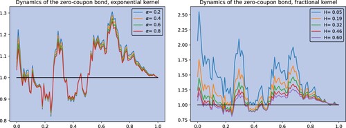
4.1. Zero-coupon dynamics

In figure 4, we analyze the impact of the parameter, α in the Exponential kernel case (section 2.3.1) and H in the Riemann-Liouville case (section 2.3.2), on the dynamics of the zero-coupon bond over a time span $[0,1]$ and considering a constant curve $\theta (\cdot )=6\mathrm{\%}$. In order to compare them properly, the underlying Brownian path is the same for all kernels. Unsurprisingly, we observe that the Riemann-Liouville case creates a lot more variance in the dynamics.

Figure 4. Dynamics of the zero-coupon bond in the Exponential (left) and the Riemann-Liouville (right) kernel case.

4.2. Impact of the roughness on convexity

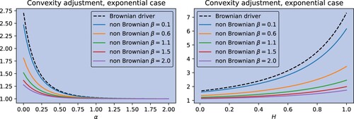
We compare in figure 5 the impact of the (roughness of the) kernel on the convexity adjustment. We consider a constant curve $\theta (\cdot )=6\mathrm{\%}$ and $(t,{\mathfrak{t}}_1,{\mathfrak{t}}_2,\tau )=(1,2,3,2)$. As α tends to zero (exponential kernel case) and as H tends to $\frac{1}{2}$ (Riemann-Liouville case), the convexity adjustments converge to the same value (as expected), approximately equal to 2.718. In figure 6, we consider example 2.4.2, shifting away from a standard Brownian driver.

Figure 5. Left: Impact of the exponential factor α on the convexity for the Exponential kernel from section 2.3.1. Right: Impact of the Hurst exponent H on the convexity for the power-law kernel from section 2.3.2.

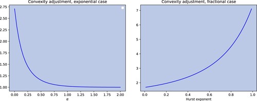
Figure 6. Left: Impact of the exponential factor α on the convexity for the Exponential kernel with standard Brownian motion (black dashed) and with OU driver with different β parameters. Right: Same but with the power-law kernel.

Acknowledgments

The authors would like to thank Damiano Brigo for helpful comments. ‘For the purpose of open access, the author(s) has applied a Creative Commons Attribution (CC BY) licence (where permitted by UKRI, “Open Government Licence” or “Creative Commons Attribution No-derivatives (CC BY-ND) licence” may be stated instead) to any Author Accepted Manuscript version arising’.

Disclosure statement

No potential conflict of interest was reported by the author(s).

Additional information

Funding

AJ is supported by the EPSRC [grant numbers EP/W032643/1 and EP/T032146/1].

Notes

1 Data available at WRDS/OptionMetrics.

2 Data available at home.treasury.gov/resource-center/data-chart-center/interest-rates.

References

- Alòs, E., Mazet, O. and Nualart, D., Stochastic calculus with respect to Gaussian processes. Ann. Probab., 2001, 29, 766–801.
- Andersen, L. and Piterbarg, V., Interest Rate Modeling, 2010 (Atlantic Financial Press).
- Basse-O'Connor, A. and Graversen, S.-E., Path and semimartingale properties of chaos processes. Stoch. Process. Appl., 2010, 120, 522–540.
- Bayer, C., Friz, P. and Gatheral, J., Pricing under rough volatility. Quant. Finance, 2016, 16, 887–904.
- Bayer, C., Friz, P.K., Fukasawa, M., Gatheral, J., Jacquier, A. and Rosenbaum, M., Rough Volatility, 2023 (SIAM).
- Bonesini, O., Jacquier, A. and Pannier, A., Rough Volatility, Path-Dependent PDEs and Weak Rates of Convergence, 2023. arXiv:2304.03042.
- Brigo, D. and Mercurio, F., Interest Rate Models-Theory and Practice: With Smile, Inflation and Credit, Vol. 2, 2006 (Springer).
- Brotherton-Ratcliffe, R. and Iben, B., Yield curve applications of swap products. In Advanced Strategies in Financial Risk Management, edited by R.J. Schwartz and C.W. Smith, pp. 400–450, 1993 (New York Institute of Finance: New York).
- El Euch, O., Fukasawa, M. and Rosenbaum, M., The microstructural foundations of leverage effect and rough volatility. Finance Stoch., 2018, 22, 241–280.
- Flesaker, B., Arbitrage free pricing of interest rate futures and forward contracts. J. Futures Mark., 1993, 13, 77–91.
- Fukasawa, M., Volatility has to be rough. Quant. Finance, 2021, 21, 1–8.
- García-Lorite, D. and Merino, R., Convexity Adjustments à la Malliavin, 2023. arXiv:2304.13402.
- Gatheral, J., Jaisson, T. and Rosenbaum, M., Volatility is rough. Quant. Finance, 2018, 18, 933–949.
- Hull, J. and White, A., Pricing interest-rate-derivative securities. Rev. Financ. Stud., 1990, 3, 573–592.
- Jacquier, A., Muguruza, A. and Pannier, A., Rough Multifactor Volatility for SPX and VIX Options, 2021. arXiv:2112.14310.
- Jacquier, A. and Oumgari, M., Deep curve-dependent PDEs for affine rough volatility. SIAM J. Financ. Math., 2023, 14, 353–382.
- Kirikos, G. and Novak, D., Convexity conundrums: Presenting a treatment of swap convexity in the hall-white framework. Risk Mag., 1997, 10, 60–61.
- Øksendal, B., Stochastic Differential Equations, 2003 (Springer).
- Pelsser, A., Mathematical foundation of convexity correction. Quant. Finance, 2003, 3, 59–65.
- Ritchken, P. and Sankarasubramanian, L., Averaging and deferred payment yield agreements. J. Futures Mark., 1993, 13, 23–41.
- Russo, F. and Tudor, C.A., On bifractional Brownian motion. Stoch. Process. Appl., 2006, 116, 830–856.
- Vasicek, O., An equilibrium characterization of the term structure. J. Financ. Econ., 1977, 5, 177–188.