Earnings mean reversion and dynamic optimal capital structure

Abstract

We formulate a trade-off model that integrates mean reversion in earnings, encompassing dynamic financing decisions that entail both the initial leverage selection and the subsequent decision related to the financing of a growth option. We identify that higher earnings mean reversion speed increases both initial and subsequent leverage ratios for growth option financing and accelerates investment, revealing the volatility-mitigating role of mean reversion speed. Furthermore, our analysis reveals a U-shaped relation between profitability and leverage, influenced by the presence of growth options. In contrast, higher long-term profitability has a positive relationship with leverage, highlighting the differential impact of long-term versus contemporaneous profitability on leverage. The model also yields further implications for corporate policies regarding debt priority structure, investment timing, default thresholds, and credit spreads, contingent on earnings mean reversion dynamics. Our empirical analysis reveals the prevalence of mean reversion in earnings among US firms and provides a comparison of capital structure decisions of firms with mean reverting earnings against firms having non-stationary earnings dynamics.

Keywords:

• Leverage
• Temporary and permanent shocks
• Real options
• Debt financing

JEL Classification:

• G31
• G13

1. Introduction

Financial flexibility is a critical consideration for firms, as emphasized by Graham and Harvey (2001) and Graham (2022). Dynamic models that incorporate adjustments in leverage and real investments offer valuable insights into firms’ capital structure decisions, as discussed by Strebulaev (2007) and analysed in various other theoretical models (e.g. Hennessy and Whited 2005, Titman and Tsyplakov 2003, Hackbarth and Mauer 2012, Shibata and Nishihara 2012, Mauer and Sarkar 2005). However, establishing a connection between the nature of earnings shocks (temporary or permanent) and firms’ financial choices remains a complex and ongoing research challenge.

A recent and growing literature is placing an increasing focus on the nature of shocks recognizing the different implications they have on corporate policies (e.g. see DeMarzo et al. 2012, Décamps et al. 2017, Gryglewicz et al. 2020, Gryglewicz et al. 2022, Hackbarth et al. 2022). Existing empirical research (Byun et al. 2019, Gryglewicz et al. 2022) underscores diverse persistence in earnings changes, while lenders adapt, based on the permanence of these shifts (Ma et al. 2022). Acknowledging this, our study examines corporate investment and financing choices using a dynamic trade-off model, centring our analysis on mean reversion to capture the range of earnings change permanence.

Mean reversion is employed in the context of energy commodities (Schwartz 1997, Geman 2005), making it a prominent feature in research focused on energy-intensive sectors (Moreno et al. 2019, Schmeck 2021). Beyond energy, Sarkar and Zapatero (2003) highlight its applicability to a broader set of industries capturing competitive dynamics, where rivals could erode advantages and restore typical earnings over time. Regardless of full characterization, variable mean reversion speeds can represent diverse permanence of earnings shocks, offering insights into corporate policies (Sarkar and Zapatero 2003).

We develop a model with arithmetic mean-reverting (AMR) earnings, incorporating dynamic financing and a growth option. Our model, unlike Levendorskii (2005) and Briest et al. (2022), who use AMR for investment options involving energy projects, focuses on the study of investment and capital structure decisions. Sarkar and Zapatero (2003) develop a trade-off model incorporating earnings mean reversion; however, their framework does not incorporate a growth option, multiple debt issues and alternative priority rules. Instead, following Hackbarth and Mauer (2012), in our model the firm has two debt issue decisions (initially and when it finances the exercise of the growth option), a priority structure decision (for the initial and subsequent debt issue), an investment decision (when to exercise the growth option), and two default decisions (before and after the exercise of the growth option). Our multi-issue debt framework, which encompasses growth option financing, contributes to the comprehension of capital structure choices made by firms during the execution of their growth options (Purnanandam and Rajan 2018). Contrary to geometric mean-reverting (GMR) process used in some literature (Sarkar 2003, Tsekrekos 2010, Metcalf and Hasset 1995 and Sarkar and Zapatero 2003) we employ an AMR which permits negative earnings and features a volatility which is independent of earnings level.¹ A comparison of our AMR assumption with earlier literature provides insights into the differences in firm behaviour due to the process assumption. Notably, with our AMR process, we obtain a negative relationship between profitability and leverage, similar to Sarkar and Zapatero (2003) who used GMR. However, our results show more significant positive adjustments in coupon payments as profitability increases compared to their GMR assumption. Our dynamic framework provides additional insights, summarized succinctly below.

Our initial predictions concern leverage ratios’ cross-sectional variation. We find that both initial and subsequent ratios (upon growth option exercise) rise with earnings mean reversion speed. This indicates a volatility-reducing effect of high mean reversion favouring greater leverage. In line with Sarkar and Zapatero (2003) we find that leverage is negatively associated with profitability in the absence of growth options. However, in contrast to Sarkar and Zapatero (2003), our research reveals a U-shaped connection between current profitability and leverage arising due to the presence of growth options. This pattern remains consistent even when considering very low mean reversion speeds as a representation of a non-stationary process. We find that long-term profitability is associated with higher leverage ratios, aligning with common expectations, underscoring the divergent effects of long-term and current profitability on leverage. In alignment with earlier empirical findings, we also discover greater leverage for firms with lower earnings volatility, as well as increased debt conservatism among growth companies. Furthermore, our investigation delves into the impact of debt priority structures. Under a ‘me-first’ priority system, we observe higher debt conservatism, leading to reduced leverage compared to an equal priority structure. Innovatively, our analysis extends to predictions concerning leverage adjustments as firms exercise growth options, revealing that lower growth option-related leverage increases occur with higher mean reversion speeds.

Our framework also adds several new corporate investment and default timing policy implications. Firstly, we demonstrate that a higher degree of mean reversion prompts investment acceleration. Secondly, we show that optimal investment timing is delayed for firms with earnings which are more volatile, have lower levels of current or long-term profitability, low levels of expansion (growth) options and for firms with a ‘me-first’ debt priority structure. Thirdly, the optimal default threshold is found to be U-shaped with respect to long-term profitability and mean reversion speed. Default is optimally delayed for firms with higher earnings volatility, higher levels of growth options and when firms have ‘me-first’ priority rule debt structure (compared with par-passu). Finally, we discuss how the interaction of firm’s investment and default policies along with capital structure affect the credit spreads.

Our valuation framework shows the impact of the earnings mean reversion and other parameters on firm value. In line with intuition, higher levels of long-term profitability, current profitability and the expansion factor for the growth option increase firm value. A less intuitive effect is obtained for the effect of mean reversion speed, where we show that similarly with volatility it has a U-shape effect on firm value. Finally, we demonstrate that a ‘me-first’ debt priority structure results in an improvement of firm value relative to an equal priority rule.

In the empirical part of the paper we focus on a sample of US firms with available observations (which account for 18% of the universe of US firms) and test for the presence of mean reversion in the data using an Augmented Dickey Fuller test. Our analysis based on the levels of earnings shows that a significance fraction of the sample, amounting to 58% of the sample, can be characterized as mean reverting. Our industry break down shows that mean reversion exists in various industries. We also provide descriptive statistics of estimates of mean reversion parameters including mean reversion speeds, long-term profitability and volatility for our sample and a comparison of firm characteristics (e.g. leverage, profitability, size) of mean reverting and non-stationary firms.

Our multivariate empirical analysis reveals that the theoretical analysis predictions are plausible. Importantly, mean reverting firms are more leveraged compared to non-stationary firms in line with model predictions showing higher leverage ratios for firms with higher speed of mean reversion. In addition, there is a more pronounced negative relation between profitability and leverage for mean reverting compared to non-stationary firms (consistent with our context and that of Sarkar and Zapatero 2003). Finally, in line with our model’s reverse of the relationship of profitability with leverage at high profitability levels driven by growth options indicating a U-shape, we show evidence of a positive adjustment of the profitability-leverage relation for firms with higher growth potential.

Related literature and contributions. Our work contributes to the literature investigating the impact of transitory and permanent earnings shocks on corporate financial policies. Compared to Gorbenko and Strebulaev (2010), who present a contingent claim trade-off model incorporating both temporary and permanent shocks featuring Poisson jumps, our approach focuses on a mean reversion process. Furthermore, we expand upon their findings regarding the debt conservatism puzzle linked to earnings dynamics revealing that the impact of mean reversion speed on leverage ratios depends on firms’ long-term profitability.

While Raymar (1991) examines dynamic decisions in a mean reversion context, his focus is on short-term (single period) debt and exogenous default. In contrast, Sarkar and Zapatero (2003) endogenize equity holders’ default decisions but in a single-stage model with no growth option. Glover and Hambusch (2016) study a single stage of financing of a growth option and focus on agency conflicts in a mean reversion context. In comparison to these earlier studies on capital structure in a mean reversion context, our analysis incorporates a growth option, two stages of financing, and endogenous default, offering a more comprehensive framework. Notably, our approach facilitates comparisons with Hackbarth and Mauer (2012), offering a comprehensive view of capital structure predictions encompassing both non-stationary and stationary earnings processes in a dynamic environment. For example, we demonstrate that the higher debt conservatism shown in Hackbarth and Mauer (2012) under ‘me-first’ priority structure of debt (compared to equal priority) is preserved in the presence of mean reversion. Conversely, our novel finding of a U-shape relationship between profitability and leverage shown in our mean reverting setting holds even for low mean reversion speeds and can thus be considered a general result irrespective of earnings dynamics.

Our work complements existing literature on earnings shock nature, which covers areas like cash holding, liquidity management and dividends (Décamps et al. 2017, Gryglewicz et al. 2022, Cadenillas et al. 2007), and agency conflicts, optimal compensation, and investment within dynamic moral hazard models (DeMarzo et al. 2012, Gryglewicz et al. 2020, Hackbarth et al. 2022). Our framework stands out by focusing on leverage dynamics, offering a novel approach to studying the effect of permanence of earnings shocks. Unlike other models, such as Décamps et al. (2017) who focus on a framework with correlated permanent and temporary shocks or Gorbenko and Strebulaev (2010) focusing on Poisson shocks, our approach models earnings using a parsimonious mean reversion process. In addition, our analysis highlights the interplay between mean reversion speed and long-term profitability, yielding new insights.

Besides our own empirical analysis, additional empirical evidence corroborates with our model predictions. Byun et al. (2019) identify temporary and persistent shocks to cash flows by applying filter methods demonstrating that firms with greater exposure to permanent cash flow shocks, i.e. shocks which are more persistent, maintain higher leverage. They also observe that firms increase debt issuance after experiencing positive permanent cash flow shocks, while the increase is much less pronounced with temporary shocks. Ma et al. (2022) reveal that lenders react differently to temporary versus permanent shifts in profitability, granting more flexibility to borrowers facing temporary changes to meet covenants. Their empirical findings underscore the importance of considering the nature of earnings shocks, as this is a feature priced by lenders. Beyond earnings shock permanence, understanding firm heterogeneity in the permanence of debt ratios is also of paramount importance for a better understanding of individual corporate capital structures (e.g. see Bontempi and Golinelli 2012).

A notable theoretical finding challenges the conventional interpretation of the empirical negative correlation between profitability and leverage. This observation, often cited against trade-off models and in favour of pecking order theory (Shyam-Sunder and Myers 1999), has been termed the ‘leverage-profitability puzzle’ (e.g. Frank and Goyal 2015). Sarkar and Zapatero (2003) single period trade-off framework, suggest a negative relation exists when earnings are mean reverting. Our contribution expands on this by considering growth options, revealing a U-shaped leverage-profitability relationship. Alternative models aiming to understand the leverage-profitability puzzle include Tserlukevich (2008), Goldstein et al. (2001) and Danis et al. (2014) who focus on fixed costs and irreversibility, explaining the negative relation due to a mechanical negative correlation of leverage and profitability in inactive periods. Graham and Leary (2011) focus on an alternative explanation of the negative profitability-leverage relation attributed to a substitution effect between operating leverage and financial leverage. Our U-shape prediction is distinct, pertaining to active financing decisions and holding regardless of the speed of mean reversion of earnings.

Our paper is organized as follows. Section 2 describes the theoretical model with mean reversion in earnings and a growth option. Section 3 presents the numerical sensitivity results and summarizes the model predictions, as well as provides comparable predictions for firms following non-stationary earnings. Section 4 presents our empirical analysis for identifying the presence of mean reversion among US firms’ earnings as well as the comparison of leverage choices of mean reverting against non-stationary firms. An Appendix provides details for the derivation of the theoretical model and an online appendix additional sensitivity tests.²

2. The model with mean reversion in earnings

2.1. Model assumptions

We model a firm with existing assets generating an earnings stream x which follows an arithmetic mean-reverting (AMR) process as follows: (1) $\mathrm{dx}=q\left(\theta -x\right)\mathrm{dt}+\mathrm{\sigma dz}$(1) where q defines the mean reversion speed, θ defines the long-term mean to which earnings revert, σ the project earnings volatility and dz is the increment to a standard Brownian Motion process. The firm has a growth opportunity to increase earnings to a level $e\cdot x$ at an optimal time. The firm selects an optimal level of perpetual debt $\mathrm{Db}\left(x\right)$ at time zero (stage 1) with a promised (coupon) payment $R_0$ and pays corporate taxes at a constant rate $\tau$ with a full-loss offset scheme.³

The bankruptcy trigger $x_b$ is endogenously and optimally chosen by equity holders by maximizing equity value. When earnings $x$ drop to the low threshold level $x_b$ then the firm goes bankrupt and the original debt holders take over and obtain the firm’s unlevered assets $\mathrm{Ub}\left(x\right)$ net of proportional bankruptcy costs b, 0 < b < 1. On the other hand, if earnings rise to a high level $x_I$ then the firm makes a capital (growth) investment I and expands earnings by e > 1, thus earnings after investment become $v=e\cdot x$. The optimal timing for investment is chosen to maximize the market value of equity (‘second-best investment’). Post investment earnings also follow a mean-reverting process of the following form: (2) $\mathrm{dv}=q\left(\mathrm{e\theta }-v\right)\mathrm{dt}+\mathrm{e\sigma dz}$(2) Thus, after investment, earnings follow an AMR process with standard deviation $e\cdot \sigma$ and long-term mean $e\cdot \theta$.

New investment can be financed by additional perpetual debt $\mathrm{Da}\left(x\right)$ with coupon $R_1$. Post investment, equity holders select the earnings level $v_L$ which triggers bankruptcy. Priority rules define the amount of unlevered assets obtained by original and subsequent debt holders in the event of bankruptcy. Like Hackbarth and Mauer (2012) we allow for commonly observed priority rules which include absolute priority of original debt, pari-passu (equal priority) and absolute priority for subsequent debt holders.

The optimal capital structure is chosen among $R_0$ and $R_1$ combinations satisfying optimally chosen investment and default timing conditions. From these $R_0$ and $R_1$ combinations we select the one that maximizes initial firm value. Note that at investment, $R_1$ is chosen to also satisfy an optimization condition maximizing the equity plus the proceeds from the new debt issue. This amounts to ‘second-best financing’, as suggested in Hackbarth and Mauer (2012). We do not focus on the study of agency issues in this paper and thus do not consider a comparison with a ‘first-best’ optimization for either the selection of investment timing and/or financing (see Hackbarth and Mauer 2012 for further details). Table 1 provides details all the variables and abbreviations used in the paper.

Table 1. Definition of variables of the theoretical model.

$\mathrm{Eb}\left(x\right)$ = Equity before investment (equity in stage 1).

$\mathrm{Fb}\left(x\right)$ = Firm value before investment.

$\mathrm{Ub}\left(x\right)$ = Value of unlevered assets before investment.

$\mathrm{TBb}\left(x\right)$ = Tax benefits before investment.

$\mathrm{BCb}\left(x\right)$ = Bankruptcy costs before investment.

$\mathrm{Db}\left(x\right)$ = Debt before investment.

$R_0$ =  Coupon for $\mathrm{Db}\left(x\right)$.

$x_b$ = Bankruptcy threshold before investment.

$x_I$ = Investment trigger

$\mathrm{Ea}\left(x\right)$ = Equity after investment (equity in stage 2).

$\mathrm{Fa}\left(x\right)$ = Firm value after investment.

$\mathrm{Ua}\left(x\right)$ = Value of unlevered assets after Investment.

$\mathrm{TBa}\left(x\right)$ = Tax Benefits after Investment.

$\mathrm{BCa}\left(x\right)$ = Bankruptcy costs after Investment.

$D{a}_0\left(x\right)$ = Debt value of debt obtained at time zero after investment.

$D{a}_1\left(x\right)$ = Debt value of debt obtained at the investment trigger after investment.

$R_1$ =  Coupon for $D{a}_1\left(x\right)$.

$x_L$ = Bankruptcy threshold following investment (in stage 2).

$\tau$ = Corporate tax rate

$b$ = Proportional to unlevered assets bankruptcy costs

${\text{β}}_0$ = share of initial debt holders at bankruptcy in stage 2 under equal priority.

${\text{β}}_1=$ share of second debt holders at bankruptcy in stage 2 under equal priority.

I = Investment cost

RT = R0 + R1

Levb = $\mathrm{Db}\left(x\right)$ / $\mathrm{Fb}\left(x\right)$: Leverage ratio at t = 0

Crb = R0/ $\mathrm{Db}\left(x\right)$-r: Credit spread of initial debt at t = 0

Invb = $\text{I }\cdot \text{ J}\left(\text{x}\right)$ = Expected present value of investment costs

NBb(x) = $\mathrm{TBb}\left(x\right)$ – $\mathrm{BCb}\left(x\right)$: Net benefits of debt

At the investment trigger:

LevT = $\left(D{a}_0\right(x\left)\text{ + }D{a}_1\right(x)$) / $\mathrm{Fa}\left(x\right)$: Total leverage ratio at the investment trigger

ΔLev = LevT-Levb: Change in leverage relative to initial stage

Crb = R0/$D{a}_0\left(x\right)$-r: Credit spread of initial debt at the investment trigger

CrT = (R0 +R1)/ ($D{a}_0\left(x\right)+D{a}_1\left(x\right))$-r: Credit spread of total debt at the investment trigger

2.2. Security and firm valuation after investment

In Appendix 1 we show the derivation of the solutions to the homogeneous differential equations with AMR. Below, we utilize the solution of the basic claims derived in Appendix 2 to simplify the exposition for the value of all claims. Appendix 3 provides full details relating the valuation of all claims.

2.2.1. Equity and unlevered assets after investment

Equity value after investment is equal to: (3) $\mathrm{Ea}\left(v\right)=E{a}_p\left(v\right)-E{a}_p\left(v_L\right)\left(\frac{P_1\left(v\right)}{P_1\left(v_L\right)}\right)$(3) where $v=\mathrm{ex}$ are expanded cash flows following investment and (4) $E{a}_p\left(v\right)=\left(\frac{1}{q+r}v+\frac{q{\theta }^{\ast }}{r\left(q+r\right)}-\frac{R_0+R_1}{r}\right)\left(1-\tau \right)$(4) with ${\theta }^{\ast }=e\cdot \theta$.

Note that in equation (3) the term $Q\left(v\right)=\frac{P_1\left(v\right)}{P_1\left(v_L\right)}$ is derived in Appendix A2.1 and can be interpreted as the value of a basic claim which pays one dollar when $v_L$ is reached from above from $v$. Equation (3) has an intuitive interpretation. It includes the present value of after tax income net of the payments to debt holders (first term) with an adjustment for income lost in the event of default (second term).

We now summarize the calculation of the basic claim $Q\left(v\right)=\frac{P_1\left(v\right)}{P_1\left(v_L\right)}$ used in equation (3). The term $P_1(\cdot )$ is defined in equation (5a) below. Equation (5b) also defines $P_2(\cdot )$ that will be used in subsequent equations for the value of securities. (5a) $\begin{array}{rl}{P}_1\left(x\right)& =e^{\frac{1}{4}{\left(\frac{\left(x-\theta \right)\sqrt{2q}}{\sigma }\right)}^2}{D}_{\nu }\left(\frac{\left(x-\theta \right)\sqrt{2q}}{\sigma }\right)\end{array}$(5a) (5b) $\begin{array}{rl}{P}_2\left(x\right)& =e^{\frac{1}{4}{\left(\frac{\left(x-\theta \right)\sqrt{2q}}{\sigma }\right)}^2}{D}_{\nu }\left(-\frac{\left(x-\theta \right)\sqrt{2q}}{\sigma }\right).\end{array}$(5b) where (6) $\begin{array}{rl}{D}_{\nu }\left(z\right)& =\frac{1}{2^{\xi }\sqrt{\pi }}[\cos (\mathrm{\xi \pi }\left)\mathrm{\Gamma }\left(\frac{1}{2}-\xi \right)y_1\right(a,z)\\ & -\sqrt{2}\sin \left(\mathrm{\xi \pi }\right)\mathrm{\Gamma }\left(1-\xi \right)y_2\left(a,z\right)]\end{array}$(6) $z=\frac{x-\theta }{\overline{\sigma }},\overline{\sigma }=\sigma /\sqrt{2q}$ $a=-\nu -\frac{1}{2},\nu =-\frac{r}{q}<0$ $\xi =\frac{1}{2}a+\frac{1}{4}$ $\mathrm{\Gamma }(\cdot )=\text{ is the Gamma function}$ $y_1\left(a,z\right)=e^{-\frac{z^2}{4}}{}_1^{}{F}_1^{}\left(\frac{1}{2}a+\frac{1}{4};\frac{1}{2};\frac{z^2}{2}\right)$ $y_2\left(a,z\right)=z{e}^{-\frac{z^2}{4}}{}_1^{}{F}_1^{}\left(\frac{1}{2}a+\frac{3}{4};\frac{3}{2};\frac{z^2}{2}\right)$

In the above ${}_1^{}{F}_1^{}\left(\alpha ;\text{β};z\right)=M\left(\alpha ;\text{β};z\right)$ is the confluent hypergeometric function (see Abramowitz and Stegun 1972). The Gamma function is defined as follows: $\mathrm{\Gamma }\left(n\right)={\int }_0^{\mathrm{\infty }}{x}^{n-1}{e}^{-x}\mathrm{dx}$ where the integral converges for n > 0. Note that $\mathrm{\Gamma }\left(n+1\right)=n\mathrm{\Gamma }\left(n\right)$, so for integer n this function coincides with the factorial function, that is, $\mathrm{\Gamma }\left(n+1\right)=n!$.

The value of unlevered assets after investment, included in the value of equity in equation (3), is shown separately below: (7) $\mathrm{Ua}\left(v\right)=\left[\frac{1}{q+r}v+\frac{q{\theta }^{\ast }}{r\left(q+r\right)}\right]\left(1-\tau \right)$(7) It is worth focusing on the impact of mean reversion on the value of assets in expression (7). The term $\frac{1}{q+r}v$ represents the transitory component and the constant $\frac{q{\theta }^{\ast }}{r\left(q+r\right)}$ is a permanent component. Note that when q = 0, then expression (7) simplifies to $\frac{v\left(1-\tau \right)}{\text{r}}$, which is the value for an arithmetic process with zero drift. When the earnings level changes, the value $\mathrm{Ua}\left(v\right)$ is affected only by the transitory part. Since the transitory part is a decreasing function of the speed of reversion q, if mean reversion becomes stronger (q increases), the transitory part becomes less important and if q goes to infinity, it disappears.

To avoid negative liquidation values for initial debt holders at bankruptcy we ensure that the value of unlevered assets after investment ($\mathrm{Ua}\left(v\right)$), as well as before investment ($\mathrm{Ub}\left(x\right)$), do not drop below zero at the bankruptcy thresholds (see Appendix 3 equations A29 and A44).

2.2.2. Debt and firm value after investment

Debt value after investment for the initial debt issued at time zero $D{a}_0\left(v\right)$ and the second debt issued at the investment trigger $D{a}_1\left(v\right)$ are given by: (8) $D{a}_i\left(v\right)=\frac{R_i}{r}+\left(D{a}_i\left(v_L\right)-\frac{R_i}{r}\right)\left(\frac{P_1\left(v\right)}{P_1\left(v_L\right)}\right)$(8) where $D{a}_i\left(v_L\right)$ defines liquidation proceeds value at bankruptcy which depends on the priority structure. The value of debt for initial and second debt issue in expression (8) includes the perpetual value of coupons (first term) and an adjustment for the event of bankruptcy (second term). In the case of equal priority of the two debt issuers, liquidation proceeds are shared depending on the scale of payments: ${\text{β}}_0=\frac{R_0}{R_0+R_1},{\text{β}}_1=1-{\text{β}}_0=\frac{R_1}{R_0+R_1}$ Thus, with equal priority the boundary condition for debt becomes: (9) $D{a}_i\left(v_L\right)={\text{β}}_i\left(1-b\right)\mathrm{Ua}\left(v_L\right)$(9) In the case the first lender has secured priority to other creditors (‘me-first’ for initial debt) then the boundary conditions become: (10a) $\begin{array}{rl}D{a}_0\left(v_L\right)& =\text{min}\left[\left(1-b\right)\mathrm{Ua}\left(v_L\right),\frac{R_0}{r}\right]\end{array}$(10a) (10b) $\begin{array}{rl}D{a}_1\left(v_L\right)& =\left(1-b\right)\mathrm{Ua}\left(v_L\right)-D{a}_0\left(v_L\right)\end{array}$(10b) In the case that second lender have secured priority to other creditors then the boundary conditions become: (11a) $\begin{array}{rl}D{a}_1\left(v_L\right)& =\text{min }\left[\left(1-b\right)\mathrm{Ua}\left(v_L\right),\frac{R_1}{r}\right]\end{array}$(11a) (11b) $\begin{array}{rl}D{a}_0\left(v_L\right)& =\left(1-b\right)\mathrm{Ua}\left(v_L\right)-D{a}_1\left(v_L\right)\end{array}$(11b) Firm value after investment is then given by the sum of equity plus debt values after investment: (12a) $\mathrm{Fa}\left(v\right)=\mathrm{Ea}\left(v\right)+D{a}_0\left(v\right)+D{a}_1\left(v\right)$(12a) Replacing equation (3) and equations (8) for $\mathrm{Ea}\left(v\right),D{a}_0\left(v\right)$ and $D{a}_1\left(v\right)$ in equation (12a) above we obtain an alternative characterization of firm value as follows: (12b) $\mathrm{Fa}\left(v\right)=\mathrm{Ua}\left(v\right)+\mathrm{TBa}\left(v\right)-\mathrm{BCa}\left(v\right)$(12b) where $\mathrm{Ua}\left(v\right)$ is given in equation (7). The expected present value of tax benefits $\mathrm{TBa}\left(v\right)$ and bankruptcy costs $\mathrm{BCa}\left(v\right)$ following investment are defined as follows:

$\mathrm{TBa}\left(v\right)=\left(\frac{R_0+R_1}{r}\right)\tau -\left(\frac{R_0+R_1}{r}\right)\tau \left(\frac{P_1\left(v\right)}{P_1\left(v_L\right)}\right)$, $\mathrm{BCa}\left(v\right)=\mathrm{bUa}\left(v_L\right)\left(\frac{P_1\left(v\right)}{P_1\left(v_L\right)}\right)$.

We define $\mathrm{NBa}\left(x\right)=\mathrm{TBa}\left(v\right)-\mathrm{BCa}\left(v\right)$ as a summary measure of the net benefits of debt after investment.

2.3. Valuation before investment

2.3.1. Equity and unlevered value before investment

Equity value before investment $\mathrm{Eb}\left(x\right)$ is given by: (13) $\begin{array}{rl}\mathrm{Eb}\left(x\right)& =\left(\mathrm{Ea}\left(e{x}_I\right)-I+D{a}_1\left(e{x}_I\right)-E{b}_p\left(x_I\right)\right)J\left(x\right)\\ & -E{b}_p\left(x_b\right)L\left(x\right)+E{b}_p\left(x\right)\end{array}$(13) where $E{b}_p\left(x\right)=\left(\frac{1}{q+r}x+\frac{q{\theta }^{}}{r\left(q+r\right)}-\frac{R_0}{r}\right)\left(1-\tau \right)$.

$J\left(x\right)$ in equation (13) defines the value of a basic claim that pays one dollar if x hits trigger $x_I$ and zero when it hits $x_b$. Similarly, we define a basic claim $L\left(x\right)$ that pays one dollar if x hits trigger $x_b$ and zero when it hits $x_I$. The solutions to these basic claims are as follows (see Appendix 1 and 2): (14) $J\left(x\right)=\frac{P_2\left(x_b\right)}{D\left(x_I,x_b\right)}{P}_1\left(x\right)-\frac{P_1\left(x_b\right)}{D\left(x_I,x_b\right)}{P}_2\left(x\right)$(14) $L\left(x\right)=-\frac{P_2\left(x_I\right)}{D\left(x_I,x_b\right)}{P}_1\left(x\right)+\frac{P_1\left(x_I\right)}{D\left(x_I,x_b\right)}{P}_2\left(x\right)$ where $D\left(x_I,x_b\right)=P_1\left(x_I\right)P_2\left(x_b\right)-P_1\left(x_b\right)P_2\left(x_I\right)$.

Note that using the above basic claims provides a very intuitive interpretation for the value of equity before investment in equation (13). The first term multiplied by $J\left(x\right)$ includes the expected value obtained from exercising the growth option investment. The second term multiplied by $L\left(x\right)$ reflects foregone income for equity holders if the default trigger is reached. The last term includes the perpetual income generated from assets at t = 0.

The value of unlevered assets before investment which is important to determine the liquidation proceeds for initial debt holders in the event of bankruptcy is given by: (15) $\mathrm{Ub}\left(x\right)=\left[\frac{1}{q+r}x+\frac{\mathrm{q\theta }}{r\left(q+r\right)}\right]\left(1-\tau \right)$(15)

2.3.2. Debt and firm value before investment

Initial (t = 0) debt value is given by: (16) $\begin{array}{rl}\mathrm{Db}\left(x\right)& =\frac{R_0}{r}+\left(D{a}_0\left(x_I\right)-\frac{R_0}{r}\right)J\left(x\right)\\ & +\left(\left(1-b\right)\mathrm{Ub}\left(x_b\right)-\frac{R_0}{r}\right)L\left(x\right)\end{array}$(16) where equation for $D{a}_0\left(x\right)$ is given in equation (8) and $\mathrm{Ub}\left(x\right)$ in equation (15).

Thus, firm value before investment is the sum of equity plus debt before investment: (17a) $\mathrm{Fb}\left(x\right)=\mathrm{Eb}\left(x\right)+\mathrm{Db}\left(x\right)$(17a) Replacing equation (13) for $\mathrm{Eb}\left(x\right)$ and equation (16) for $\mathrm{Db}\left(x\right)$ we obtain the following breakdown of firm value at t = 0: (17b) $\begin{array}{rl}\mathrm{Fb}\left(x\right)& =\mathrm{UB}\left(x\right)+\mathrm{Ua}\left(v_I\right)J\left(x\right)+\mathrm{TBb}\left(x\right)+\mathrm{TBa}\left(v_I\right)J\left(x\right)\\ & -\mathrm{BCb}\left(x\right)-\mathrm{BCa}\left(v_I\right)J\left(x\right)-\mathrm{IJ}\left(x\right)\end{array}$(17b) where $\mathrm{UB}\left(x\right)=\mathrm{Ub}\left(x\right)-\mathrm{Ub}\left(x_I\right)J\left(x\right)$ with $\mathrm{Ub}(\cdot )$ given in equation (15), $\mathrm{TBb}\left(x\right)=\frac{\tau R_0}{r}-\frac{\tau R_0}{r}J\left(x\right)-\frac{\tau R_0}{r}L\left(x\right)$ and $\mathrm{BCb}\left(x\right)=\mathrm{bUb}\left(x_b\right)L\left(x\right)$. We also define the net benefits of debt at t = 0 as $\mathrm{NBb}\left(x\right)=\mathrm{TBb}\left(x\right)-\mathrm{BCb}\left(x\right)$.

Expression (17b) for firm value underscores the trade-off nature of the model by decomposing firm value into the value of unlevered assets, tax benefits of debt and bankruptcy costs.

2.4. Optimal investment, default, and capital structure

In this section we describe smooth pasting (optimality) conditions. First, we demand that the derivative of equity after investment at $v_L$ should be zero to ensure that equity holders choose the bankruptcy trigger optimally following investment. This implies the condition: (18) $E{a}^{\mathrm{\prime }}\left(v_L\right)=0.$(18) Note that the optimality condition in equation (18) can be stated in terms of the underlying x with the condition $\tilde{E}{a}^{\mathrm{\prime }}\left(x_L\right)=0$ where $\tilde{E}a(\cdot )$ is equation defined in equation (3) evaluated at $v=\mathrm{ex}$. Similarly, we demand that the derivative of equity value before investment should be zero at bankruptcy trigger $x_b$: (19) $E{b}^{\mathrm{\prime }}\left(x_b\right)=0.$(19)

We use ‘second-best investment’ optimization for the investment trigger $x_I$ which accounts for raising the optimal new level of debt financing, however, it does not account for the effect of investment on existing debt holders. This translates into: (20) $E{b}^{\mathrm{\prime }}\left(x_I\right)=\tilde{E}{a}^{\mathrm{\prime }}\left(x_I\right)+\tilde{D}{a_1}^{\mathrm{\prime }}\left(x_I\right)$(20) Note that under ‘first-best investment’ optimization (not used in our subsequent analysis) equity holders consider the best interest of debt issuers by optimizing firm value. This would imply the following condition $F{b}^{\mathrm{\prime }}\left(x_I\right)=\tilde{F}{a}^{\mathrm{\prime }}\left(x_I\right)$ where $\tilde{F}{a}^{\mathrm{\prime }}\left(x_I\right)$ is equation (12) replacing $v=e\cdot x$. ‘First-best investment’ would be useful for analysing agency issues which is not the goal of this paper.

The optimal capital structure is selected numerically by performing a double-loop dense grid search for both the initial and subsequent coupon levels $R_0$ and $R_1$. For each $R_0$ and $R_1$ combination, we ensure the satisfaction of optimally chosen default levels conditions (see equations 18, 19) and the smooth pasting condition at the investment trigger (equation 20). From these $R_0$ and $R_1$ combinations, satisfying the optimality conditions, we select the one that maximizes initial firm value, that is the equity plus initial debt financing obtained (see equation, 17a). This optimization process establishes the initial and subsequent debt levels in the firm's capital structure.

3. Model predictions

3.1. Sensitivity analysis

In this section, we offer numerical sensitivity analyses concerning key parameters, relating to mean reversion speed (q), long-term profitability (θ), earnings level (x), volatility (σ), growth option expansion factor (e), and the influence of alternate debt priority rules. Our investigation delves into their effects on firm value, leverage ratio levels, changes in leverage ratios upon exercise of the growth option, and credit spreads. We also emphasize the formulation of empirical predictions amenable to empirical testing concerning cross-sectional leverage ratios.

Our base case parameters are as follows. We use a normalized level of current earnings at the level $x=1$. Following Hackbarth and Mauer (2012) we use a risk-free rate of $r=0.06$, a tax rate $\tau =0.15$. For the growth option we also follow the same study and use $e=2$ and an investment cost $I=10$ (i.e. the cost of investment is ten times the current earnings level as used in Hackbarth and Mauer 2012). We take proportional bankruptcy costs $b=0.5$ as in Leland (1994). For the mean-reverting stochastic process parameters we follow Sarkar and Zapatero (2003) and use $\sigma =0.4$, mean reversion speed $q=0.1$ and long-term mean $\theta =1$.⁴

For all subsequently reported results we report sensitivity until $x<x_I$ remains valid. In all simulations we ensure that the value of unlevered assets at default thresholds which defines recovery values for debt holders at default (net of bankruptcy costs) is never negative (see discussion following equations A29 and A44 in the Appendix 3). Finally, where necessary to show a particular direction of an effect more clearly, we provide a denser sensitivity analysis.

Table 2 provides new insights regarding the impact of mean reversion speed (q). We observe that an increase in mean reversion speed q leads to a reduction in $x_I$, implying an acceleration of investment. This effect holds true regardless of long-term levels of profitability. The acceleration of investment is discernible not only through the decreased $x_I$ at higher mean reversion speeds (refer to Panel A) but also through the elevated expected investment ($\mathrm{In}{v}_b\left(x\right)$) for greater q values (refer to Panel B). Our findings extend the work of Sarkar and Zapatero (2003) into an investment option context. The accelerated investment pattern aligns with a real options rationale, where a higher mean reversion speed indicates a less volatile earnings process.

Table 2. Sensitivity analysis with respect to mean reversion speed (q).

Panel A: Optimal coupon and thresholds
Base case (θ = 1)
q	R0	R1	xI	vL	xb
0.10	0.52	0.55	1.341	−1.501	−1.191
0.15	0.65	0.45	1.238	−1.795	−1.209
0.20	0.78	0.45	1.149	−1.810	−1.134
0.25	0.88	0.47	1.077	−1.738	−1.053
0.30	0.96	0.49	1.021	−1.623	−0.958
Lower long-term profitability (θ = 0.75)
q	R0	R1	xI	vL	xb
0.10	0.36	0.54	1.473	−1.356	−1.094
0.15	0.39	0.4	1.409	−1.772	−1.186
0.20	0.46	0.37	1.342	−1.947	−1.169
0.25	0.52	0.39	1.276	−1.969	−1.137
0.30	0.57	0.42	1.217	−1.910	−1.094
Panel B: Firm value, equity, debt and leverage and credit spreads
Base case (θ = 1)
	Values at t = 0							Values at investment trigger T
q	Fb(x)	Db(x)	Eb(x)	Ub(x)	NBb(x)	Levb	Invb	Crb	LevT	ΔLev	CrT
0.1	20.556	7.997	8.518	26.720	1.692	0.389	7.856	0.005	0.485	0.096	0.0052
0.15	20.771	10.486	7.046	27.234	2.174	0.505	8.637	0.002	0.545	0.040	0.0020
0.2	21.166	12.787	6.114	27.683	2.707	0.604	9.224	0.001	0.628	0.024	0.0010
0.25	21.524	14.526	5.244	28.019	3.139	0.675	9.634	0.0006	0.698	0.023	0.0006
0.3	21.814	15.898	4.605	28.253	3.469	0.729	9.908	0.0004	0.752	0.023	0.0004
Lower long-term profitability (θ = 0.75)
	Values at t = 0							Values at investment trigger T
q	Fb(x)	Db(x)	Eb(x)	Ub(x)	NBb(x)	Levb	Invb	Crb	LevT	ΔLev	CrT
0.1	16.063	5.239	10.823	21.488	1.167	0.326	6.591	0.0087	0.431	0.104	0.0089
0.15	15.227	6.118	9.104	21.037	1.261	0.402	7.072	0.0037	0.44	0.038	0.0041
0.2	14.954	7.448	7.505	20.95	1.573	0.498	7.568	0.0018	0.499	0.001	0.0019
0.25	14.876	8.53	6.345	21.052	1.897	0.573	8.073	0.001	0.569	−0.004	0.0010
0.3	14.863	9.404	5.459	21.207	2.176	0.633	8.521	0.0006	0.633	0.001	0.0006

Notes: Initial earnings level x = 1, risk-free rate r = 0.06, tax rate τ = 0.15, proportional bankruptcy costs b = 0.5, growth option rate e = 2, investment cost I = 10. For the mean-reverting stochastic model parameters we use σ = 0.4, long-term mean θ = 1 or θ = 0.75 and vary mean reversion speed q. ΔLev stands for change in leverage and is calculated as Lev_T – Lev_b. Base case parameters highlighted in bold.

Our results also extend the work of Sarkar and Zapatero (2003) within a dynamic capital structure framework encompassing initial and subsequent leverage decisions. Consistent with the role of mean reversion speed in reducing volatility, we discover that both initial coupons and leverage rise with the speed of mean reversion. The positive correlation between leverage and q is evident even at the investment trigger stage, when firms transition to a phase devoid of further growth options. Furthermore, our analysis builds upon Gorbenko and Strebulaev (2010) by offering deeper insights into the favorable impact of mean reversion speed on leverage. Specifically, we reveal that the higher leverage ratio for higher q values is influenced by the alternative impact in the valuations of both equity and debt, contingent on the company's long-term profitability. In instances of strong long-term profitability, an elevated q leads to increases in the leverage ratio arising from increases in debt value despite the increase in overall firm value (denominator of the leverage ratio), suggesting that debt increases at a higher rate than firm value increases. Conversely, when long-term profitability is low, we observe that leverage increases both because debt increases but also because the overall firm value (the denominator of the leverage ratio) decreases.

Our context also extends earlier literature by providing predictions with respect to the effect of speed of mean reversion on leverage dynamics. For instance, Purnanandam and Rajan (2018) investigate how optimal growth option exercise serves to transmit project quality information to the market, thereby diminishing the relative cost of issuing information-sensitive financial claims. Our analysis offers insights into capital structure changes during growth option execution, influenced by earnings dynamics. We observe that an increase in the speed of mean reversion results in a lower increase of leverage at the investment threshold relative to the initial level. This effect holds irrespective of long-term profitability level. Intuitively, the lower increase in leverage ratios relate to the lower $x_I$ level at which investment options are exercised when the speed of mean reversion is high implying a lower debt capacity. Credit spreads decrease as the speed of mean reversion increases for both the base case of long-term profitability θ and the case where θ is low, which is also consistent with the fact that a higher q implies lower volatility.

Understanding how a firm’s value is influenced by the speed of earnings mean reversion is important for both the management of these firms and for potential investors. We find that the speed of mean reversion results in a reduction in equity value and an increase in debt value. The effect of speed of mean reversion on firm value depends on the level of firm’s long-term profitability. Specifically, in the base case where long-term profitability is high, we found that firm value increases as the speed of mean reversion increases. However, in situations where long-term profitability is low (see case $\theta$ = 0.75), we observed the opposite effect, where the firm's value decreases with an increase in the speed of mean reversion. Thus, more generally one should expect a U-shape for intermediate values of long-term profitability. Such a U-shape can be explained with reference to the effect of speed of mean reversion on volatility which shows a similar U-shape relation with leverage.

We now turn to the effect of long-term profitability.⁵ In line with intuition, Table 3 shows that an increase in long-term profitability (θ) accelerates a firm’s investment as indicated by the lower $x_I$ (see panel A) and the higher expected investment costs (Inv_b(x)) (see panel B) and, as expected, increases firm value by increasing both equity and debt values.

Table 3. Sensitivity analysis with respect to long-term profitability (θ).

Panel A: Optimal coupon and thresholds
θ	R0	R1	xI	vL	xb
0.6	0.31	0.53	1.571	−1.217	−0.974
0.75	0.36	0.54	1.473	−1.356	−1.094
1	0.52	0.55	1.341	−1.501	−1.191
1.25	0.73	0.58	1.237	−1.544	−1.234
1.5	0.99	0.61	1.156	−1.504	−1.210
1.75	1.29	0.63	1.093	−1.411	−1.132
2	1.64	0.62	1.047	−1.282	−0.976
2.25	2.03	0.57	1.017	−1.161	−0.764
Panel B: Firm value, equity, debt and leverage and credit spreads
	Values at t = 0							Values at investment trigger T
θ	Fb(x)	Db(x)	Eb(x)	Ub(x)	NBb(x)	Levb	Invb	Crb	LevT	ΔLev	CrT
0.6	13.635	4.246	9.387	18.243	0.97	0.311	5.578	0.013	0.405	0.094	0.0126
0.75	16.063	5.238	10.823	21.488	1.167	0.326	6.591	0.0087	0.430	0.104	0.009
1	20.556	7.997	12.555	26.72	1.692	0.389	7.856	0.005	0.485	0.096	0.0052
1.25	25.429	11.561	13.867	31.741	2.396	0.455	8.708	0.0031	0.548	0.093	0.0032
1.5	30.532	15.923	14.601	36.579	3.214	0.522	9.261	0.0022	0.611	0.089	0.0022
1.75	35.763	20.952	14.808	41.283	4.093	0.586	9.613	0.0016	0.667	0.081	0.0016
2	41.063	26.787	14.265	45.883	5.004	0.652	9.824	0.0012	0.716	0.064	0.0012
2.25	46.398	33.325	13.071	50.414	5.928	0.718	9.944	0.0009	0.754	0.036	0.0009

Notes: Initial earnings level x = 1, risk-free rate r = 0.06, tax rate τ = 0.15, proportional bankruptcy costs b = 0.5, growth option rate e = 2, investment cost I = 10. For the mean-reverting stochastic model parameters we use σ = 0.4, mean reversion speed q = 0.1 and vary long-term mean of earnings θ. ΔLev stands for change in leverage and is calculated as Lev_T – Lev_b. Base case parameters highlighted in bold.

Table 3 shows that long-term profitability increases the initial leverage ratio, as well as the leverage ratio when the investment option is exercised. Studies building on static versions of the trade-off model for empirical investigation (see, e.g. Frank and Goyal 2009; Graham and Leary 2011) have associated leverage ratios with contemporaneous (not long-term) profitability, finding a puzzling negative relation. Our theoretical context brings clarity by helping to explain the different impact of a firm's current versus long-term profitability on leverage ratios. Indeed, our subsequent sensitivity analysis on contemporaneous profitability shows that it has a different impact on leverage ratios compared to long-term profitability.

With respect to leverage dynamics, we find that leverage increases at a lower rate with respect to the level of long-term profitability. This result is driven by the lower threshold where investment takes place when long-term profitability is high which supports lower debt levels. Consistent with intuition, higher long-term profitability results in lower credit spreads at the investment threshold. Long-term profitability has a U-shape with respect to default thresholds $v_L$ and $x_b$.

While long-term profitability has an intuitive positive effect on leverage ratios, the effect of contemporaneous (current) profitability on leverage is quite different. Table 4 shows that a negative relation between leverage and current profitability levels (see panel B) for the base case parameters holds for a wide range of x values, while for high values of x, the relation becomes positive, suggesting more broadly a U-shape relation between leverage and contemporaneous profitability.

Table 4. Sensitivity analysis with respect to current profitability level (x).

Panel A: Optimal coupon and thresholds
x	R0	R1	xI	vL	xb
−0.40	0.30	0.8	1.323	−1.481	−1.660
−0.25	0.32	0.8	1.324	−1.481	−1.616
0	0.37	0.7	1.327	−1.481	−1.508
0.25	0.41	0.7	1.330	−1.481	−1.422
0.50	0.44	0.6	1.332	−1.481	−1.358
0.75	0.48	0.6	1.336	−1.501	−1.274
1	0.52	0.6	1.341	−1.501	−1.191
1.25	0.59	0.5	1.352	−1.501	−1.049
1.30	0.62	0.45	1.357	−1.501	−0.989
1.35	0.68	0.4	1.369	−1.481	−0.873
Panel B: Firm value, equity, debt and leverage and credit spreads
	Values at t = 0							Values at investment trigger T
x	Fb(x)	Db(x)	Eb(x)	Ub(x)	NBb(x)	Levb	Invb	Crb	LevT	ΔLev	CrT
−0.4	10.391	4.583	5.807	13.44	1.176	0.441	4.225	0.0055	0.492	0.051	0.0054
−0.25	11.372	4.912	6.458	14.596	1.225	0.432	4.449	0.0051	0.491	0.059	0.0054
0	13.039	5.688	7.351	16.576	1.318	0.436	4.855	0.0051	0.491	0.055	0.0053
0.25	14.762	6.31	8.449	18.716	1.407	0.427	5.361	0.005	0.491	0.064	0.0054
0.5	16.563	6.78	9.780	21.069	1.493	0.409	6.000	0.0049	0.490	0.081	0.0053
0.75	18.476	7.393	11.079	23.688	1.589	0.4	6.801	0.0049	0.486	0.086	0.0052
1	20.556	7.997	12.555	26.720	1.692	0.389	7.856	0.005	0.485	0.096	0.0052
1.25	22.882	9.05	13.824	30.322	1.807	0.396	9.247	0.0052	0.484	0.088	0.0052
1.3	23.389	9.509	13.872	31.118	1.832	0.407	9.561	0.0052	0.483	0.077	0.0052
1.35	23.915	10.418	13.489	31.908	1.856	0.436	9.848	0.0053	0.485	0.05	0.0052

Notes: Risk-free rate r = 0.06, tax rate τ = 0.15, proportional bankruptcy costs b = 0.5, growth option rate e = 2, investment cost I = 10. For the mean-reverting stochastic model parameters we use σ = 0.4, mean reversion speed q = 0.1 and long-term mean of earnings θ = 1. ΔLev stands for change in leverage and is calculated as Lev_T – Lev_b. Base case parameters highlighted in bold.

The negative relationship between profitability and leverage commonly observed in the literature (see, e.g. Frank and Goyal 2009; Graham and Leary 2011) plausibly prevails across a broad range of profitability levels or when growth options are not significant. An alternate explanation, extensively supported in the literature, attributes the negative correlation to firms’ hesitancy in adjusting leverage due to the presence of costly adjustment expenses (as elaborated in models by Fischer et al. 1989; Goldstein et al. 2001, Strebulaev 2007, Danis et al. 2014) or to a substitution effect between operating leverage and financial leverage (Graham and Leary 2011). However, our prediction deviates, prompting empirical investigation to center around the impact of mean reversion causing, or exasperating, the observed negative impact, which is expected to be reversed in the presence of growth options (see empirical section).

Our prediction for the presence of U-shape, extends the work of Sarkar and Zapatero (2003), showing that in the presence of growth options at high current profitability, this relationship may be inverted, resulting in a more rapid increase in debt values compared to equity values—thereby leading to an elevated leverage ratio. This U-shaped pattern remains consistent across alternative parameterizations, encompassing diverse scenarios of long-term profitability and mean-reversion speeds (additional results are detailed in an online Appendix). Furthermore, this U-shaped correlation is preserved even in cases where q→0, signifying its applicability to firms with restricted mean reversion and approximating non-stationary earnings dynamics. Our supplementary analysis in online Appendix 2 confirms the persistence of the U-shaped profitability-leverage relationship in firms following Geometric Brownian Motion (GBM) in earnings—such as the setting presented in Hackbarth and Mauer (2012).

It is noteworthy that while empirical studies often consider the return on assets as opposed to profit levels, our constructed theoretical measure of return on assets, defined as earnings scaled by unlevered assets (Ub(x)), also conforms to the U-shaped pattern in relation to leverage—a fact readily confirmed (refer to Figure 1).

Figure 1. The theoretical cross sectional relationship between leverage and return on asset.

Note: The figure uses numerical sensitivity results from the theoretical model in Table 4. The y-axis is Levb and the x-axis is a theoretical measure of return on assets taken as $x\left(1-\tau \right)/\mathrm{Ub}\left(x\right)$ which defines the after tax earnings divided by the value of unlevered assets Ub(x).

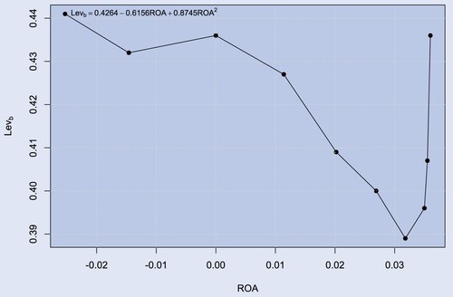
The U-shaped relationship between profitability and leverage within our framework has the following underpinnings. In the range of low profitability and a relatively out-of-the-money growth option, increased profitability results in a relatively modest increase in debt compared to equity. This restrained increase in debt arises due to the temporary nature of earnings increases, driven by the prevailing impact of mean reversion. Conversely, within this low profitability spectrum, equity registers a more rapid rise. This occurs from equity's encompassment of options, both favorably toward the realization of growth prospects and for truncation of downside losses concerning the choice of the timing of default. In contrast, as profitability reaches elevated levels, the likelihood of exercising the growth option increases, facilitating the firm's entering into an expanded revenue level. This, in turn, enhances the firm's debt capacity while equity increase flats out, culminating in higher leverage ratios.

We further explore the influence of growth options on this relationship by examining scenarios without growth options (refer to online Appendix 3). Our findings demonstrate that in the absence of a growth option, the relationship becomes negative for higher x values, thus lacking the U-shaped pattern. Evidently, the growth option serves as the primary catalyst behind the U-shaped relation between leverage and profitability. This U-shaped pattern was also discernible in Raymar (1991). However, Raymar (1991) focuses on short-term debt which exasperates the positive effect on leverage of an increase in profitability. Moreover, in Raymar (1991) default is exogenous, while we allow for endogenous default.

Notably, this observed U-shape would likely exhibit greater prominence compared to utilizing a Geometric Mean Reversion (GMR) (e.g. as in Sarkar and Zapatero 2003). This is due to the GMR process leading to higher volatility when earnings become higher (which reduces leverage at higher earnings levels), a phenomenon absent in our framework with Arithmetic Mean Reversion (AMR) which maintains earnings volatility constant irrespective of earnings levels. Indeed, a comparison of our AMR assumption with that of GMR performed in online Appendix 3 shows a more significant increase in coupon levels as profitability increases under an AMR process compared to the case of GMR.

We proceed to analyze the implications of a firm's response to an increase in current earnings on its investment and default strategies. As shown in Table 4, Panel A, the investment threshold experiences an ascent alongside x, albeit with an accompanying acceleration in investment due to the relatively moderate growth in the investment trigger compared to the incremental rise in x. This investment acceleration is further highlighted by the amplified value of expected investment costs ($\mathrm{In}{v}_b\left(x\right)$), as illustrated in Panel B.

Regarding default thresholds, Panel A demonstrates the increase of $x_b$ with x, whereas $v_L$ slightly diminishes. These effects are determined by the firm's decisions regarding coupon levels $R_0$ and $R_1$. Specifically, $R_0$ displays an increase, while $R_1$ sees a decline in relation with x. In line with expectations, Table 4, Panel B, shows that an increase in current profitability expands firm and debt values, along with the net benefits of debt. The succinct summary of the effects of current profitability on leverage adjustments and credit spreads is provided in Table 6.

Table 5 presents sensitivity analyses concerning earnings volatility (σ). In Panel A, aligned with a real options reasoning, increased volatility results in a postponement of the investment option ($x_I$ rises) and a delay in default choices ($v_L$ and $x_b$ thresholds decline). In Panel B, the impact of higher earnings volatility is U-shaped on firm value (Fb(x)) driven by the opposite effects of volatility on equity value (positive) compared to debt value (negative). Higher volatility also leads to diminished value of unlevered assets (Ub(x)), reduced leverage ratio at t = 0 ($\mathrm{Le}{v}_b$), decreased net benefits of debt (NB(x)), and lowered anticipated present value of investment costs ($\mathrm{In}{v}_b$). This last effect implies a reduced likelihood of investment occurrence. As anticipated, leverage falls with volatility, extending the findings of Sarkar and Zapatero (2003) within a dynamic context.

Table 5. Sensitivity analysis with respect to earnings volatility (σ).

Panel A: Optimal coupon and thresholds
σ	R0	R1	xI	vL	xb
0.24	0.72	0.46	1.015	−0.658	−0.415
0.30	0.61	0.5	1.135	−1.028	−0.772
0.40	0.52	0.55	1.341	−1.501	−1.191
0.50	0.46	0.64	1.541	−1.856	−1.563
Panel B: Firm value, equity, debt and leverage and credit spreads
	Values at t = 0							Values at investment trigger T
σ	Fb(x)	Db(x)	Eb(x)	Ub(x)	NBb(x)	Levb	Invb	Crb	LevT	ΔLev	CrT
0.24	20.822	11.644	9.175	28.187	2.475	0.559	9.84	0.0018	0.616	0.057	0.0018
0.3	20.58	9.711	10.867	27.373	2.08	0.472	8.873	0.0028	0.553	0.081	0.0028
0.4	20.556	7.997	12.555	26.72	1.692	0.389	7.856	0.005	0.485	0.096	0.0052
0.5	20.815	6.778	14.034	26.551	1.532	0.326	7.268	0.0079	0.45	0.124	0.0082

Notes: Initial earning level x = 1, risk-free rate r = 0.06, tax rate τ = 0.15, proportional bankruptcy costs b = 0.5, growth rate parameter e = 2, investment cost I = 10. For the mean-reverting stochastic model parameters we vary σ and use a mean reversion speed q = 0.1 and long-term mean of earnings θ = 1. ΔLev stands for change in leverage and is calculated as Lev_T – Lev_b. Base case parameters are highlighted in bold.

Despite the leverage decrease, credit spreads rise with σ, echoing the increased debt riskiness. Elevated volatility also curtails leverage ratios and positively impacts credit spreads at the investment trigger. In terms of leverage dynamics, we show that when firms reach the investment-execution stage without remaining options, leverage surpasses prior levels when volatility is higher. This pattern is intuitively linked to higher volatility facilitating investment initiation at elevated revenue thresholds, thus enabling the firm to transition toward higher leverage levels.

We've also investigated whether the sensitivity outcomes mentioned above, about the effect of earnings volatility, change with varying levels of long-term profitability (tables not included for brevity). Our findings reveal that, in instances of high long-term profitability, an increase in volatility diminishes firm value. This result is intuitive, as increased volatility raises the probability of deviating from highly valuable prospects. Conversely, when long-term profitability is low, the firm value demonstrates a strictly increasing relation with volatility. This accounts for the U-shaped pattern observed in our baseline scenario of (average) long-term profitability. Despite these divergences from our baseline, all other findings remain consistent with higher level of volatility: investment and default is delayed, leverage contracts, credit spreads increase, and adjustments in leverage at the investment trigger in relation to previous levels intensify.

Finally, we report sensitivity outcomesof the growth option expansion factor and capital investment cost (tables not presented for conciseness). A higher level of the growth expansion factor hastens investment, defers default, and enhances firm value by increasing both equity and debt value. Despite the enhanced net benefits of debt, the leverage ratio at t = 0 diminishes. This outcome aligns with the well-documented debt conservatism observed in firms with growth options (Graham and Harvey 2001). Notably, coupon levels rise at t = 0, yet the more substantial improvement in equity value compared to debt contributes to the reduction in the leverage ratio. The inverse relationship between market leverage and growth options also aligns with Hackbarth and Mauer (2012), who employ a Geometric Brownian Motion for earnings under a second-best solution framework, akin to our model.⁶ Conversely, we observe an increased leverage ratio with the expansion factor as firms reach a stage where they exercise their investment growth options. Notably, there is a more pronounced rise in credit spreads at this later stage. In contrastto the effects described for the expansion factor, we notice opposite directional impacts concerning the level of capital investment cost (I).

In online Appendix 1, we provide sensitivity results and discussions concerning the optimal priority rule. Similar to Hackbarth and Mauer (2012), we observe that adopting a ‘me-first’ priority rule for initial debt leads to enhanced firm values, increased debt conservatism, and greater underinvestment compared to scenarios where alternative debt issuances possess equal priority.

3.2. Summary of empirical predictions and comparison with models with non-stationary earnings

Table 6 summarizes model predictions for firms exhibiting earnings mean reversion, intended as guidance for empirical analysis.

Table 6. Summary of directional effects on firm value, firm investment and default policies and leverage dynamics.

Parameter	Fb(x)	xI	vL	xb	Levb	LevT	ΔLev
Volatility (σ) ^1	U	+	–	–	–	–	+
Mean reversion speed (q)^2	U	–	U	U	+	+	–
Long-term profitability (θ)	+	-	U	U	+	+	-
Earnings level (x)	+	+	-	+	U	-	Inverted U
Growth expansion factor (e)	+	-	-	-	-	+	+
Capital investment cost (I)	-	+	+	+	+	-	-
Me-first priority rule (compared with equal priority)	+	+	-	-	-	Minor positive	+

Notes: The above table summarizes our sensitivity results. Note 1: the relation holds for ‘average’ long-term profitability: firm value is increasing when long-term profitability is low and decreasing when long-term profitability is high. All other effects of volatility remain unchanged. Note 2: When long-term profitability is low (high) firm value is decreasing (increasing).

Empirical focus often centers on cross-sectional determinants of leverage ratios. Thus, we succinctly present our primary empirical leverage predictions for mean-reverting firms (refer to $\mathrm{Le}{v}_b$ in Table 6⁷).

Comparing our model predictions with those involving non-stationary earnings is illuminating. A comparison suggests a similarity in the cross sectional predictions across various factors irrespective of earnings dynamics. Specifically, Hackbarth and Mauer (2012) also establish a negative association between market leverage and volatility, as well as a negative correlation with the value of growth opportunities. Similarly, lower leverage is observed under a ‘me-first’ debt priority rule compared to equal priority scenarios. Since their analysis did not include the effect of profitability, in online Appendix section 2, we present results following the Hackbarth and Mauer (2012) paper, affirming that the U-shaped profitability-leverage relation for firms operating also exists under Geometric Brownian Motion (GBM) in earnings.⁸

The above discussion highlights that a number of variables are expected to behave similarly in the cross section, irrespective of earnings dynamics, in line with the similarity in the mechanisms underlying trade-off models. Despite the similarities, however, there are potential differences between the behavior of mean reverting and non-stationary firms which we explore empirically in the next section.

First, we are interested in understanding any potential differences between mean reverting versus non-stationary firms in the choice of leverage levels. The positive impact of the mean reversion speed on leverage on both at initial and follow-on stages involving the financing of growth options (see Tables 1 and 6) is illuminating, suggesting that stronger levels of mean reversion will result in higher leverage ratios in the cross section. This leads to the following hypothesis:

H1 (Leverage of mean reverting vs non-stationary firms): Leverage ratios for mean reverting firms are expected to be higher compared to firms exhibiting no mean reversion (non-stationary firms).

Secondly, we focus on potential differences in the profitability-leverage relation. The empirical literature on capital structure has identified a negative relation between profitability and leverage which is attributed to firms’ inaction in frequently adjusting leverage causing a mechanical negative relation of profitability with leverage (e.g. Danis et al. 2014). Excluding a growth option, our model predicts, similarly to Sarkar and Zapatero (2003), that the impact of mean reversion should result in an exasperation of the negative relation of profitability with leverage (in contrast, in the absence of growth options leverage ratios do not vary with profitability under non-stationary dynamics as also discussed Sarkar and Zapatero 2003). However, our analysis when adding growth option suggests that the negative relation observed in the cross section is plausible even without reference to inaction irrespective of earnings dynamics. Specifically, our analysis suggests that adding multiple stages of financing involving the financing of a growth option results in a wide region where the profitability exhibits a negative relation with leverage for both mean reverting firms and non-stationary firms (see online appendix 2 for the latter). We can summarize the following hypotheses that considers also the effect of growth options:

H2a (Profitability-leverage relation): Leverage is anticipated to have a negative relation with profitability for mean reverting and non-stationary firms (due to inaction or multiple stages of financing involving growth options causing a wide range of negative relation). The negative effect is expected to be more pronounced for the mean reverting group.

H2b (Impact of growth options on profitability-leverage relation): We expect that a mitigation of the negative profitability-leverage effect for high profitability levels exists for firms facing high growth potential for either mean reverting or non-stationary firms.

Finally, in our model and our sensitivity analysis concerning the case with non-stationary dynamics, the effect of growth options (as indicated by our sensitivity of expansion factor of the growth option) leads to more conservative leverage ratios. A similar effect exists also in the case of non-stationary dynamics leading to the following hypothesis where the differences in the reaction of the two groups will be explored empirically.

H3: (Growth options impact): Growth options (proxied by market-to-book) are expected to have a negative relation on leverage irrespective of earnings dynamics.

4. Empirical analysis

4.1. Mean reversion process estimation and descriptive statistics for mean-reverting and non-stationary firms

The solution of the stochastic differential equation in eq. (1) implies the following discrete approximation for the dynamics of x (see Dixit and Pindyck 1994, 76, eq.19): (21) $\mathrm{\Delta }{x}_t=\theta \left(1-e^{-q}\right)+(e^{-q}-1)x_{t-1}+\sigma \sqrt{\frac{1-e^{-2q}}{2q}}{Z}_t$(21) where $Z_t\sim N\left(0,1\right)$. In the above specification the standard error per unit of interval is: (22) ${\sigma }_{ϵ}=\sigma \sqrt{\frac{1-e^{-2q}}{2q}}$(22) To estimate the mean reversion speed (q), long-term mean (θ) and volatility (σ) in equation (21) we estimate the following AR (1) model in discrete time (see Dixit and Pindyck 1994, 76): (23) $\mathrm{\Delta }{x}_t=a+b{x}_{t-1}+{ϵ}_t$(23) We then associate the estimated terms with the continuous time model approximation analogue in equation (21) which results in the following solution for the parameters: (24) $\begin{array}{rl}q& =-\text{ln}\left(1+\hat{b}\right)\end{array}$(24) (25) $\begin{array}{rl}\theta & =-\frac{\hat{a}}{\hat{b}}\end{array}$(25) (26) $\begin{array}{rl}\sigma & ={\sigma }_{ϵ}\sqrt{\frac{\text{ln}\left(1+\hat{b}\right)}{{\left(1+\hat{b}\right)}^2-1}}\end{array}$(26)

For preserving mean reversion, we need that $-1<\hat{b}<0$ so that we obtain a positive mean reversion speed. Note that the smaller the coefficient $\hat{b}$ the larger the speed of mean reversion q while as $\hat{b}\to 0$ we have $q\to 0$. We estimate eq. (23) after first de-seasonalizing the earnings series and after scaling each firm’s earnings with its initial sample earnings level so we have comparable results across firms.⁹ We then use an ADF test to test the null of non-stationary series $\hat{b}$ = 0 versus the alternative of stationary series $\hat{b}$<0 using a 5% level of significance. Note that ${\sigma }_{ϵ}$ can be estimated using the standard error of regression of eq. (23). We use this as an input to estimate our volatility measure for mean reverting processes as shown in eq. (26). We report ${\sigma }_{ϵ}$ as a measure of volatility risk for the case where firms are found to be non-stationary.

Our initial sample is from the quarterly COMPUSTAT database covering the period between January 1961 and June 2020. We do not go beyond 2020 so as not to introduce possible bias in our estimates arising from the effect of the COVID pandemic. We exclude financial firms (Standard Industrial Classification (SIC) codes 6000 to 6999) and regulated firms (SIC codes 4900 to 4999). The total number of non-financial and non-regulated firms in the sample before and after the requirement of at least 40 consecutive observations is shown in Table 7. Table 7 shows the detailed steps in arriving at our final sample of firms which we summarize below.

Table 7. Sample of mean reverting and non-stationary firms.

Total non-financial and non-regulated firms	26,223
Number of firms with N = 40 consecutive earnings (oibdpq) excluding firms with growth >500% and no full parameter estimates of stochastic process	4,672
N. of firms classified as mean reverting	2,694
N. of firms classified as non-mean reverting	1,978
N. of mean reverting firms used in subsequent analysis with 1% quantile and 99% quantile for long-term mean and mean reversion speed removed and those with volatility higher than 5.	2,123
N. of non-mean reverting firms with volatility higher than 5 removed.	1,641
N. of unique mean reverting firms with complete observations on all financial variables (with 1% highest and lowest outliers removed)	1,572
Total number of firm-quarter year observation with full data for mean reverting firms	67,370
N. of unique non-mean reverting firms with complete observations on all variables (with 1% highest and lowest outliers removed)	1,300
Total number of firm-quarter year observation with full data for non-mean reverting firms	58,581

Similarly to Byun et al. (2019) for a firm to be included in the analysis we require that it has at least 40 consecutive quarterly observations (10 year of data) for earnings (oibdpq).¹⁰ In addition, following Gryglewicz et al. (2022) we impose a condition for the exclusion of firms with asset growth exceeding 500%. The reasoning for exclusion of firms with significant asset growth is to exclude firms with abrupt changes in asset growth reflecting large jumps in business fundamentals (e.g. mergers, reorganizations). We also exclude a limited number of firms where a complete set of stochastic process parameter estimates was not possible. Our restrictions, necessary to conduct a reasonable classification based on ADF test, limits our sample, however it is provides a representative sample of about 18% of the overall non financial and non-regulated firms listed in the US. The sample size is similar to Byun et al. (2019) requiring similar restrictions using consecutive observations.

Table 7 also shows the number of firms classified as mean reverting using the full sample available for each firm by applying the ADF to test the null of non-stationary series (based on estimating eq. 23). Using the ADF, our analysis shows that about 58% of the firms with available data are classified as having mean reverting (stationary) earnings.

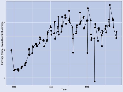
Besides the formal ADF test we have visually inspected firms’ earnings using line graphs to assess how reasonable our classification may be. Figure 2 illustratively shows a firm found to be mean-reverting and reports the estimates for the mean reverting process.

Figure 2. Example of a firm classified as mean reverting.

Notes: The figure shows an example of mean reverting firm with gvkey = 1609 with estimated parameters θ = 1.5, q = 0.23 and σe = 0.37. The figure show earnings (oibdpq) unadjusted for seasonality and scaled by the initial value of earnings of the firm for the whole periods of consecutive available data the firm.

Byun et al. (2019) focus on identifying temporary and persistent shocks to cash flows by applying the filtering methods. Hence their analysis is not directly comparable with our analysis focusing on identifying mean reversion. In addition, their analysis focuses on a scaled measured of cash flows to total assets (i.e. a return on asset measure). In contrast, our analysis is based on the level of operating income which is consistent with theoretical model assumptions and thus provides (to the best of our knowledge) the first evidence of a significant presence of earnings mean reversion in earnings levels. In contrast, Gryglewicz et al. (2022) find a significant proportion of firms following non-stationary earnings. However their analysis requires at least 10, not necessarily consecutive, observations and focuses on annual not quarterly data series. Before we proceed to create a sample to compare the financial characteristics of mean reverting and non-stationary firms we apply an additional filtering in order to remove any firms with extreme earnings process estimates of mean reversion speed, long-term mean and volatility as described in Table 7.

Our sample of firm financial variables is obtained from COMPUSTAT. We merge COMPUSTAT with CRSP monthly security prices based on the initial month of the same quarter to construct the market value of equity. We calculate market leverage, profitability (ROA), volatility, size (log sales) adjusted for inflation, market to book, tangible assets, cash ratio, capital expenditure to assets and industry concentration based on Herfindahl index (see Danis et al. (2014) and Eckbo and Kisser 2021). After trimming the 1% lowest and highest values for all variables to avoid outliers we are left with 1,572 unique mean reverting firms with complete data and a total of 67,370 firm-quarter observations on these variables. We apply the same process for the sample of non-stationary firms which leaves a sample of 1,300 unique non-stationary firms with complete data and a total of 58,581 firm-quarter observations on all variables. The final sample is summarized in Table 7.

Regarding industry characteristics (tables not shown for brevity), the data reveal that mean reverting and non-mean reverting firms are evenly split in different industries. The evidence thus does not support the hypothesis that earnings dynamics is driven by the industry the firm is operating. Most sample observations, with about 56% of our sample for mean reverting and 53% respectively for the non-stationary, belong to the manufacturing sector, followed by services with about 14% and 20% for the two groups respectively. The mining sector (a possible candidate to suspect stronger levels of mean reversion due to reliance on commodity prices) represents only 5% of mean reverting observations (a similar proportion exists also for non-mean reverting firms). We find that mean reversion (and non-stationarity) exists in other sectors such as transportation, communications, electric, gas and sanitary service and wholesale trade.

Table 8, panel A provides descriptive statistics for our sample of mean reverting firms with panel B showing related information for the sample of non-stationary firms.

Table 8. Descriptive statistics for sample of mean reverting and non-stationary firms.

Panel A: Mean reverting firms
	25% perc.	Median	Mean	75% perc.	Std
Market Leverage (gross)- Total	0.103	0.249	0.297	0.447	0.232
Profitability (ROA)	0.008	0.028	0.032	0.051	0.057
Size (Log of sales)	−3.055	−1.573	−1.542	−0.016	2.069
Market to book	0.644	0.922	1.174	1.386	0.896
Tangible assets	0.132	0.259	0.312	0.449	0.222
Herfindahl index	0.084	0.128	0.177	0.224	0.143
Cash ratio	0.019	0.060	0.111	0.150	0.137
Capex to assets (year-to-date)	0.009	0.021	0.033	0.043	0.036
Volatility (σ)	0.298	0.706	1.098	1.490	1.113
Long-Term profitability (θ)	0.407	0.989	1.426	2.097	2.223
Mean reversion speed (q)	0.347	0.566	0.751	0.928	0.594
Panel B: Non-stationary firms
	25% perc.	Median	Mean	75% perc.	Std
Market Leverage (gross)- Total	0.073	0.181	0.239	0.352	0.212
Profitability (ROA)	0.031	0.061	0.109	0.126	0.160
Size (Log of sales)	−2.015	−0.779	−0.846	0.313	1.811
Market to book	0.866	1.241	1.566	1.893	1.097
Tangible assets	0.121	0.256	0.316	0.471	0.236
Herfindahl index	0.080	0.119	0.159	0.199	0.127
Cash ratio	0.023	0.066	0.122	0.167	0.144
Capex to assets (year-to-date)	0.010	0.022	0.036	0.047	0.040
Volatility (σϵ)	0.361	0.712	1.168	1.587	1.154

Notes: The table provides descriptive statistics of all non-financial, non-regulated firms with at least 40 consecutive earnings (oibdpq) which are either mean reverting or non-stationary and have complete data on a set of variables needed for the analysis (see Table 5). Gross market leverage defined as long-term debt plus short-term debt divided long-term debt plus short-term debt plus the market value of equity, with market value of equity calculated using CRSP data (dlttq + dlcq)/ (dlttq + dlcq + price × shrout) while gross Profitability is defined as operating income after depreciation over total asset (oibdpq/atq). Volatility (σ) is the estimate of volatility as defined in eq. (29). Volatility (σ_ϵ) is defined as the estimated volatility of the standard error of eq. (26). Market-to-book is the market value of equity plus long-term debt divided by total assets ((equity + dlttq)/atq). Tangible assets are property plant and equipment over total assets (ppentq/atq). Herfindahl index a particular industry is defined as the sum of squared market shares for all firms in a two-digit SIC industry in a year-quarter. The market share of a firm is defined as sales of that firm in a year-quarter divided by the total sales in the industry of firm in that year-quarter. Cash ratio is cash and equivalents (cheq) scaled by total assets. Capex to assets is (capex) scaled by total assets. LT profitability (θ) is defined in eq. (28). Mean reversion speed is the estimated mean reversion speed as defined in eq. (27).

The sample of mean reverting firms exhibits higher leverage despite mean reverting firms being on average less profitable (in terms of ROA) compared to the corresponding non-stationary group of firms. These differences stand out and provide preliminary evidence to support our theoretical framework (see H1) where higher speeds of mean reversion result in higher leverage ratios (see Table 1 and the summary of effects in Table 6). We provide additional evidence to support this in the next subsection within a multivariate context which controls for other firm characteristics.

We turn our attention to the estimates of stochastic model parameters. First, we provide estimates of the stochastic process volatility with separate estimates for mean reverting (panel A) and non-mean reverting firms (panel B).¹¹ There is scarce evidence for comparison of our estimates concerning volatilties, however our estimate of volatility appears reasonable when compared with the analysis of Gryglewicz et al. (2022). While Gryglewicz et al. (2022) follow a different estimation approach by separately estimating the variance of the temporary and the permanent component, our estimates appear to be reasonably close to their volatility of the permanent component of earnings shocks.¹² Interestingly, our estimates for the median long-term profitability is close to par to firms’ initial earnings level. However, the long term mean profitability is almost 43% higher than firms’ initial earnings level indicating an upside long-term profitability for the mean firm. The evidence also suggests a significant persistence of earnings close to their long-term mean with an average mean reversion speed of 0.751 (a median speed of 0.566).

4.2. Multivariate analysis

In this section we empirically investigate the relation between different factors affecting leverage for our sample of mean reversion firms and non-stationary firms. For the multivariate empirical tests, we run the following linear regression: (27) $\begin{array}{rl}{L}_{i,t}& =a+{\gamma }_0\mathrm{RO}{A}_{i,t-1}+{\gamma }_1\mathrm{Siz}{e}_{\iota ,t-1}+{\gamma }_{2}M{B}_{\iota ,t-1}\\ & +{\gamma }_3\mathrm{Tan}{g}_{i,t-1}+{\gamma }_4\mathrm{Her}{f}_{i,t-1}+\text{β}\left(\mathrm{RO}{A}_{i,t-1}\cdot M{B}_{\iota ,t-1}\right)\end{array}$(27) where $L_{i,t}$ denotes gross market leverage, $\mathrm{RO}{A}_{i,t-1}$ is operating income after depreciation over total assets (ROA), $M{B}_{\iota ,t-1}$ is the market-to-book ratio, $\mathrm{Tan}{g}_{i,t-1}$ reflects firms proportion of tangible assets and $\mathrm{Her}{f}_{i,t-1}$ is the Herfindahl index showing industry concentration. The last term in the regression captures the interaction of profitability with growth opportunities aiming to investigate whether the profitability-leverage relation is affected by a firm’s growth options. The above panel regression is run separately for the mean reverting and non-reverting sample of firms and also for the full sample (including both groups). In the latter case of using the full sample we also include a dummy (called Revert) to investigate the differences in leverage decisions between mean reverting and non-mean reverting firms. We also interact this dummy with the profitability and market to book measure in order to uncover the differential impact of growth options depending on whether the firm is mean reverting or non-stationary. In all specifications we use time and industry fixed effects and heteroskedastic and autocorrelation robust standard errors clustered at firm level.

Our first goal is to see whether important factors affecting leverage used in previous empirical capital structure studies behave the same for our sub-samples of mean reverting and non-stationary firms (see models (1) and (2) respectively) (Table 9).

Table 9. Factors affecting leverage for mean reverting firms.

	Mean reverting	Non-stationary	All firms
	(1)	(2)	(3)
ROA	−0.493***	−0.123***	−0.159***
	(0.035)	(0.014)	(0.014)
Size	0.010***	0.006***	0.008***
	(0.001)	(0.001)	(0.000)
MB	−0.109***	−0.095***	−0.092***
	(0.002)	(0.001)	(0.001)
Tang.	0.168***	0.171***	0.166***
	(0.007)	(0.007)	(0.005)
Herf.	−0.036***	−0.034**	−0.024**
	(0.013)	(0.014)	(0.010)
Interaction of ROA with growth
MB × ROA	0.099***	0.053***	0.056***
	(0.019)	(0.005)	(0.005)
Revert vs Non-Revert
Revert			0.061***
			(0.010)
ROA × Revert			−0.327***
			(0.038)
MB × Revert			−0.021***
			(0.002)
ROA × MB × Revert			0.051**
			(0.02)
Quarter FE	Yes	Yes	Yes
Industry FE	Yes	Yes	Yes
R^2	0.328	0.391	0.350
Adj. R^2	0.326	0.389	0.348
Firm obs.	1,572	1,300	2,872
Total obs.	67,370	58,581	125,951
F-test (Prob)	<0.0001	<0.0001	<0.0001

Notes: The analysis is based on all non-financial, non-regulated firms with at least 40 consecutive earnings (oibdpq) (see Table 5). The dependent variable is gross market leverage defined as long-term debt plus short-term debt divided long-term debt plus short-term debt plus the market value of equity, with market value of equity calculated using CRSP data (dlttq + dlcq)/ (dlttq + dlcq + price × shrout). Profitability is defined as operating income after depreciation over total asset (oibdpq/atq). Size is the inflation adjusted log of sales (log(salesq/cpiind)). Market-to-book is the market value of equity plus long-term debt divided by total assets ((equity + dlttq)/atq). Tangible assets are property plant and equipment over total assets (ppentq/atq). Herfindahl index a particular industry is defined as the sum of squared market shares for all firms in a two-digit SIC industry in a year-quarter. The market share of a firm is defined as sales of that firm in a year-quarter divided by the total sales in the industry of firm in that year-quarter. The symbols *, **, and **** refer to estimates significantly different from zero at 10%, 5% and 1% confidence level, respectively. Heteroskedastic and autocorrelation robust standard errors clustered at firm level are provided in parenthesis.

We find that expected empirical predictions supporting trade-off models confirm other studies and hold irrespective of earnings dynamics. In both model (1) (mean reverting) and model (2) (non-stationary), the results show that leverage is negatively associated with profitability. The negative profitability-leverage is consistent with inaction causing a mechanical negative relation between the two variables (see Danis et al. 2014) and also the observed wide range of negative relation between profitability and leverage which exists in our multistage framework. This effect is expected to apply irrespective of whether the firm is mean reverting or non-stationary (see previous section leading to H2a). In addition, as expected, market-to-book (a proxy for growth options) is negatively associated with leverage whereas size and tangible assets are positively associated with leverage as in other studies (see e.g. Danis et al. 2014, Table 2, p.433). In contrast to Danis et al. (2014) we find Herfindahl industry concentration to negatively affect leverage in both groups.¹³

In line with our theoretical discussion on the impact of growth options on the leverage-profitability relation (see H2b), our last interaction variable between profitability and market to book aims to investigate whether the negative relation between leverage and profitability is mitigated due to the presence of growth options. Indeed, we find evidence of the positive influence of growth options, showing that for high growth firms the negative relation of profitability with leverage is reduced.

Model (3) reveals additional insights relating the different behavior between mean reverting and non-stationary firms. First, we confirm that the results obtained in the capital structure literature regarding the effect of profitability, size, market-to-book and tangible assets are consistent with prior literature. This is reassuring that our sample is representative of the overall population of firms. We also confirm that the leverage-profitability relation is mitigated by the presence of growth options for the overall sample.

The most revealing part of the analysis of model (3) is that mean reverting firms are more leveraged compared to non-mean reverting firms after controlling for firm characteristics. This is in line with the theoretical model (see H1) where a higher speed of mean reversion is expected to result in higher leverage (see Table 1 and Table 6). The absolute magnitude of this effect is a significant 6.1% while the relative magnitude when compared to the mean leverage for the whole sample (which is about 27%)¹⁴ showing a significant 23% more leverage for the average mean reverting compared to the mean sample firm ( = (0.061/0.27)).

The comparison of the firms reaction to profitability changes provides additional insights. First, we find that the negative relation between profitability and leverage is more pronounced for mean reverting compared to non-stationary firms (see negative coefficient of ROA x Revert). This effect is in line with our model suggesting that a negative effect relation between profitability and leverage existing for a wide range of profitability levels. Thus, besides the mechanical negative relation caused due to inaction shown in the literature, we show that mean reversion induces an additional (reinforcing) negative effect on the relation between profitability and leverage (see H2a).

Trade-off models focusing on either mean reverting or non-stationary dynamics predict higher debt conservatism (lower leverage ratios) when firms have higher growth options (see previous section leading to H3). It would be interesting however to investigate empirically which group of firms behaves more conservatively when facing higher growth potential. Our empirical analysis finds that mean reverting firms are more conservative (reduce leverage more) in reaction to increases in growth options compared to non-stationary changes (see negative sign of MB x Revert). Lastly, the interaction between profitability and growth options aims to investigate how the growth options effect on the profitability-leverage relation differs between the two groups. The empirical analysis shows that the mitigation effect of higher profitability on leverage when firms face higher growth options is more substantial for the mean reversion group. In sum, our empirical investigation provides evidence that earnings dynamics is an important determinant of firms’ capital structure decisions.

5. Conclusion

We developed a dynamic trade-off model integrating mean-reversion in earnings and leverage adjustments during the exercise and financing of a growth option. Our analysis yields novel insights into the impact of earnings dynamics, specifically long-term profitability, mean reversion speed, and volatility, on firm value, leverage levels, dynamic leverage changes, and credit spreads. Our framework also bring forth managerial implications regarding optimal investment and default timing based on model parameters and earnings process attributes.

We contribute several new insights concerning the effects of earnings shocks’ permanence and long-term profitability levels. Notably, higher mean reversion speed positively impacts current and future leverage ratios and accelerates investment. Significantly, we contrast our findings with related scenarios that centre on non-stationary earnings dynamics, elucidating predictions from dynamic trade-off models. This analysis underscores a consistent U-shaped relation between current profitability and leverage, attributable to growth options, independent of earnings dynamics. Moreover, our investigation reveals that adopting a ‘me-first’ priority structure, akin to earlier literature findings in the context of non-stationary earnings dynamics, enhances firm value yet could lead to underinvestment and more conservative debt levels.

Our empirical analysis reveals that a significant fraction of US firms spanning various industries can be well characterized as having a mean reverting earnings process. In line with our theoretical predictions, our analysis reveals that mean reverting firms have more leverage compared to non-stationary firms. We also show empirically that mean reverting firms are more conservative in their leverage choices when facing high growth options. With respect to the U-shape of profitability with leverage caused with growth options we find evidence of a more substantial effect for the mean reversion group.

Given the evidence of prevalence of mean reversion in quarterly earnings, future research avenues could consider other important topics such as managerial-shareholder conflicts, or managerial conservatism, as discussed in Graham (2022) in a dynamic mean reversion context.

Disclosure statement

No potential conflict of interest was reported by the author(s). 

Supplemental data

Supplemental data for this article can be accessed online at https://doi.org/10.1080/14697688.2024.2361018.

Notes

1 The GMR could be used to model revenues (instead of earnings) and only by properly including positive costs would allow for negative earnings. An alternative mean reversion process also used is the Cox-Ingersoll and Ross (CIR) process discussed in a real options context in Ewald and Wang (2010).

2 Specifically, Appendix 1 shows the derivation of the homogeneous differential equation solution, Appendix 2 shows the derivation of the solutions for the basic and general claims involving two boundaries within a mean-reverting framework and Appendix 3 shows the proofs for security and firm values presented in the main text. The online Appendix presents additional sensitivity results of the main model and sensitivity that confirm the robustness of the U-shape of leverage with respect to profitability, irrespective of the earnings process, as well as results of sensitivity with respect to profitability in the absence of growth option.

3 We do not consider tax convexity issues (see Sarkar 2008) but assume that constant tax rate τ is applied irrespective of the earnings level. Our analysis thus likely somehow exaggerates the true tax benefits levels.

4 The predictions derived in this section are not affected if we use the median sample empirical estimates derived in Section 4 of the volatility of earnings, mean reversion speed, and long-term profitability for all US non-regulated and non-financial firms with consecutive 10-year quarterly data.

5 This is particularly important for investors. See for example the case of Tesla: https://www.forbes.com/sites/sergeiklebnikov/2022/06/09/tesla-stock-can-jump-another-50-thanks-to-superior-growth-in-the-years-ahead-analysts-say/?sh=61363ad51f06.

6 They establish a U-shaped pattern in the first-best case, which pertains to scenarios devoid of agency conflicts. We, however, do not analyze the first-best case here, as it represents an ideal scenario without conflicts between debt and equity holders. Such an analysis would have been essential for measuring agency costs, an aspect we do not delve into in this study. Empirical evidence by Ogden and Wu (2013) explores the plausibility of a non-linear relationship between leverage and growth options (market-to-book).

7 Initial financing leverage ratios ($\mathrm{Le}{v}_b$) mirror anticipated patterns within a framework involving potential growth options. For instance, it is reasonable to expect a negative relation between market-to-book and leverage (as indicated by $\mathrm{Le}{v}_b$) in the cross-section, contrasting with a positive correlation (as in $\mathrm{Le}{v}_T$) that would only emerge if growth options vanish post an investment decision.

8 Moreover, we have conducted sensitivity analyses approximating the non-stationary case within our framework, which can be obtained when q tends to zero, verifying a similar U-shape exists for very low q. While formally our case of q→0, defining non-stationary firms, does not encompass GBM motion, our qualitative (sign) empirical predictions for q→0 align with those obtained under the assumption of a GBM motion process on earnings.

9 A related approach is adopted by Gryglewicz et al. (2022), wherein they scale each earnings observation with the initial asset level. Instead, we scale by initial earnings to maintain normalization consistent with the theoretical model, where the initial earnings level starts at x = 1. Similar to Gryglewicz et al. (2022), this normalization aids in interpreting the results more effectively and does not impact the results of the ADF test.

10 Byun et al. (2019) work with annual data. Unlike Byun et al. (2019) we do not fill missing values with nearby averages (our consecutive observation requirement is thus more strict). Gryglewicz et al. (2022) require at least 10 years, not necessarily consecutive, observations, however they employ a filtering technique that does not require the use of consecutive observations. They also subtract the change in working capital from earnings (oibdpq) stating however that their analysis is not affected by this transformation. For this reason we choose to focus on earnings without working capital adjustment which also allows maintaining consistency with our theoretical model assumptions involving no working capital adjustments.

11 Typically in capital structure studies (e.g., Danis et al. 2014) estimates of volatility are based on the standard derivation of earnings divided by the number of observations used (e.g., Danis et al. 2014 scale by 20 observations). While providing a crude approach of comparison, when scaling our estimates of volatility with the same number of quarters our results appear closer to these literature estimates.

12 Indeed, they report a median volatility of the permanent component of 65.1% with our median being 70.6% while their 75% quantile volatility is 126% while ours is 149%.

13 We note that our industry concentration measure uses a two-digit SIC code whereas Danis et al. (2014) use a four-digit SIC.

14 This can be readily seen as the weighted average of the means of the two groups’ leverage ratio with weights being the contribution of each group in the overall sample (58% for mean reverting and 42% for non-mean reverting).

15 To derive this general contingent claim differential equation, we assume risk-neutral investors and hence that the total required return on holding an asset in equilibrium is $r=a\left(x\right)+\delta$ where $a\left(x\right)=q\left(\theta -x\right)$ is the capital (gain) of asset x and $\delta$ the convenience yield. Thus, the implied convenience yield of holding the underlying asset x is $\delta =r-a\left(x\right)$. A similar approach is followed in Sarkar and Zapatero (2003).

Appendices

Appendix 1.

Derivation of the homogeneous differential equation solution

Following standard replication arguments (example, Dixit and Pindyck 1994, 180) any contingent claim $P\left(x\right)$on an underlying asset x that follows the mean reversion process defined in equation (1) should satisfy¹⁵: (A1) $T\left(P\left(x\right)\right)=\frac{1}{2}{\sigma }^2{P}^{\mathrm{\prime \prime }}\left(x\right)-q\left(x-\theta \right)P^{\mathrm{\prime }}\left(x\right)-\mathrm{rP}\left(x\right)=0,x\in \mathrm{\Re }$(A1) To find the general solution of this homogeneous differential equation first set $\overline{\sigma }=\sigma /\sqrt{2q}$ and make the following change of variables: $z=\frac{x-\theta }{\overline{\sigma }}.$ Then $P\left(x\right)=u\left(z\right),P^{\mathrm{\prime }}\left(x\right)=\frac{1}{\overline{\sigma }}{u}^{\mathrm{\prime }}\left(z\right)$ and $P^{{}^{\mathrm{\prime \prime }}}\left(x\right)=\frac{1}{\overline{{\overline{\sigma }}^2}}{u}^{\mathrm{\prime \prime }}\left(z\right)$. Thus equation (A1) is transformed to: (A2) $q{u}^{\mathrm{\prime \prime }}\left(z\right)-\mathrm{qz}{u}^{\mathrm{\prime }}\left(z\right)-\mathrm{ru}\left(z\right)=0,z\in \mathrm{\Re }.$(A2) Setting also $u\left(z\right)=w\left(z\right)e^{\frac{z^2}{4}}$, with $\nu =-\frac{r}{q}<0$, deduce that $u^{\mathrm{\prime }}\left(z\right)=e^{\frac{z^2}{4}}\left(w^{\mathrm{\prime }}\left(z\right)+w\left(z\right)\frac{z}{2}\right)$ and $u^{\mathrm{\prime \prime }}\left(z\right)=e^{\frac{z^2}{4}}\left(w^{\mathrm{\prime \prime }}\right(z)+z{w}^{\mathrm{\prime }}(z)+w(z)\frac{1}{2}\left(1+\frac{z^2}{2}\right))$. A simple calculation then shows that equation (A2) can be rewritten into: (A3) $w^{\mathrm{\prime \prime }}\left(z\right)-\left[\frac{1}{4}{z}^2-\left(\nu +\frac{1}{2}\right)\right]w\left(z\right)=0,z\in \mathrm{\Re }.$(A3) Equation (A3) is the real version of Weber’s equation (Abramowitz and Stegun 1972), that is: (A4) $w^{\mathrm{\prime \prime }}\left(z\right)-\left[\frac{1}{4}{z}^2+a\right]w\left(z\right)=0,z\in \mathbb{C},$(A4) where $a=-\nu -\frac{1}{2}$. The general solution of equation (A3) is given by: (A5) $w_g\left(z\right)=C_{1}U\left(a,z\right)+C_{2}U\left(a,-z\right).$(A5) With $C_1$ and $C_2$ general constants and where: (A6) $\begin{array}{rl}U\left(a,z\right)& =\frac{1}{2^{\xi }\sqrt{\pi }}[\cos (\mathrm{\xi \pi }\left)\mathrm{\Gamma }\left(\frac{1}{2}-\xi \right)y_1\right(a,z)\\ & -\sqrt{2}\sin \left(\mathrm{\xi \pi }\right)\mathrm{\Gamma }\left(1-\xi \right)y_2\left(a,z\right)]\end{array}$(A6) with $\xi =\frac{1}{2}a+\frac{1}{4},$ (A7) $y_1\left(a,z\right)=e^{-\frac{z^2}{4}}{}_1^{}{F}_1^{}\left(\frac{1}{2}a+\frac{1}{4};\frac{1}{2};\frac{z^2}{2}\right)$(A7) and (A8) $y_2\left(a,z\right)=z{e}^{-\frac{z^2}{4}}{}_1^{}{F}_1^{}\left(\frac{1}{2}a+\frac{3}{4};\frac{3}{2};\frac{z^2}{2}\right)$(A8) where ${}_1^{}{F}_1^{}\left(\alpha ;\text{β};z\right)=M\left(\alpha ;\text{β};z\right)$ is the confluent hypergeometric function (see Buchholz 1969, Borodin and Salminen 2002).

For the sake of being in the same line of notation with the literature concerning the limits of functions subsequently used we name $D_{\nu }\left(z\right)=U\left(a,z\right)$. Thus, focusing on the real solutions, the general solution (A5) can be re-written as: (A9) $w_g\left(z\right)=C_1{D}_{\nu }\left(z\right)+C_2{D}_{\nu }\left(-z\right)z\in \mathrm{\Re }.$(A9) Two useful asymptotic properties of the two linear independent solutions of equation (A3) (Abramowitz and Stegun (1972), equations 19.3.1 and 19.3.2, p.687, combined with equations 19.8.1 and 19.8.2, p.689) are the following: (A10) $\underset{z\to \mathrm{\infty }}{lim}{e}^{\frac{z^2}{4}}{D}_{\nu }\left(z\right)=\underset{z\to \mathrm{\infty }}{\text{lim}}{z}^{\nu }(1+O(z^{-2})=0,\mathrm{for\nu }<0$(A10) and (A11) $\underset{z\to \mathrm{\infty }}{lim}{e}^{\frac{z^2}{4}}{D}_{\nu }\left(-z\right)\sim \frac{\sqrt{2\pi }}{\mathrm{\Gamma }\left(-\nu \right)}\underset{z\to \mathrm{\infty }}{\text{lim}}{e}^{\frac{z^2}{2}}{z}^{-\nu -1}=\mathrm{\infty }.$(A11) Since we have used the transformation $u\left(z\right)=w\left(z\right)e^{\frac{z^2}{4}}$ we can now move back to get the general solution of equation (A2) to be: $u_g\left(z\right)=C_1{e}^{\frac{z^2}{4}}{D}_{\nu }\left(z\right)+C_2{e}^{\frac{z^2}{4}}{D}_{\nu }\left(-z\right),z\in \mathrm{\Re }.$ Thus, we deduce that the solution of equation (A1) expressed in terms of x is given by: (A12) $\begin{array}{rl}P\left(x\right)& =C_1{e}^{\frac{1}{4}{\left(\frac{\left(x-\theta \right)\sqrt{2q}}{\sigma }\right)}^2}{D}_{\nu }\left(\frac{\left(x-\theta \right)\sqrt{2q}}{\sigma }\right)\\ & +C_2{e}^{\frac{1}{4}{\left(\frac{\left(x-\theta \right)\sqrt{2q}}{\sigma }\right)}^2}{D}_{\nu }\left(-\frac{\left(x-\theta \right)\sqrt{2q}}{\sigma }\right),x\in \mathrm{\Re }.\end{array}$(A12) For simplicity of presentation denote the general solution of (A1) as (A13a) $P\left(x\right)=C_1{P}_1\left(x\right)+C_2{P}_2\left(x\right),$(A13a) with $P_1\left(x\right)=e^{\frac{1}{4}{\left(\frac{\left(x-\theta \right)\sqrt{2q}}{\sigma }\right)}^2}{D}_{\nu }\left(\frac{\left(x-\theta \right)\sqrt{2q}}{\sigma }\right),$ and $P_2\left(x\right)=e^{\frac{1}{4}{\left(\frac{\left(x-\theta \right)\sqrt{2q}}{\sigma }\right)}^2}{D}_{\nu }\left(-\frac{\left(x-\theta \right)\sqrt{2q}}{\sigma }\right),$ with equations (A10) and (A11) giving that: (A13b) $\begin{array}{rl}\underset{x\to \mathrm{\infty }}{\text{lim}}{P}_1\left(x\right)& =0\end{array}$(A13b) (A13c) $\begin{array}{rl}\underset{x\to -\mathrm{\infty }}{\text{lim}}{P}_1\left(x\right)& =\mathrm{\infty }\end{array}$(A13c) (A13d) $\begin{array}{rl}\underset{x\to \mathrm{\infty }}{\text{lim}}{P}_2\left(x\right)& =\mathrm{\infty }\end{array}$(A13d) (A13e) $\begin{array}{rl}\underset{x\to -\mathrm{\infty }}{\text{lim}}{P}_2\left(x\right)& =0\end{array}$(A13e)

Appendix 2.

Derivation of solution for basic and general claims involving two boundaries

A2.1. Basic claim paying one dollar at $v_L$ after investment

Consider the following differential equation problem: (A14) $T^{\ast }\left(Q\left(v\right)\right)=0,v\in \mathrm{\Re }$(A14) $\underset{v\to \mathrm{\infty }}{\text{lim}}Q\left(v\right)=0$ $Q\left(v_L\right)=1$ where $T^{\ast }\left({\theta }^{\ast },{\sigma }^{\ast }\right)\equiv T\left(\mathrm{e\theta },\mathrm{e\sigma }\right)$. The solution for $Q\left(v\right)$ is given by applying (A13a): $Q\left(v\right)=C_1{P}_1\left(v\right)+C_2{P}_2\left(v\right)$ Applying the first boundary condition in (A14) combined with equation (A13d) gives $C_2=0$. Then the second boundary condition gives $C_1=\frac{1}{P_1\left(v_L\right)}$ . Thus, the solution for this basic claim paying one dollar at $v_L$ after investment is: (A15) $Q\left(v\right)=\frac{P_1\left(v\right)}{P_1\left(v_L\right)}$(A15)

A2.1. Basic claims for homogeneous equations before investment

$J\left(x\right)$ and $L\left(x\right)$ are basic claims where $J\left(x\right)$ pays one dollar at $x_I$ and zero when $x_b$ is reached and $L\left(x\right)$ pays one dollar at $x_b$ and zero when $x_I$ is reached.

A. Derivation of $J\left(x\right)$

Consider the following differential equation problem: (A16) $T\left(J\left(x\right)\right)=0,x\in \mathrm{\Re }$(A16) $J\left(x_I\right)=1$ $J\left(x_b\right)=0$

The solution $J\left(x\right)$ satisfies (A13) hence: $J\left(x\right)=C_1{P}_1\left(x\right)+C_2{P}_2\left(x\right)$ Applying the boundary conditions in (A16) results in: $C_1=\frac{P_2\left(x_b\right)}{D\left(x_I,x_b\right)},C_2=-\frac{P_1\left(x_b\right)}{D\left(x_I,x_b\right)},$ where $D\left(x_I,x_b\right)=P_1\left(x_I\right)P_2\left(x_b\right)-P_1\left(x_b\right)P_2\left(x_I\right).$ Thus, the solution for J(x) is: (A17) $J\left(x\right)=\frac{P_2\left(x_b\right)}{D\left(x_I,x_b\right)}{P}_1\left(x\right)-\frac{P_1\left(x_b\right)}{D\left(x_I,x_b\right)}{P}_2\left(x\right).$(A17)

B. Derivation of $L\left(x\right)$

Consider now the corresponding problem for $L\left(x\right)$ which is given by: (A18) $T\left(L\left(x\right)\right)=0,x\in \mathrm{\Re }$(A18) $L\left(x_I\right)=0$ $L\left(x_b\right)=1$

Applying the boundary conditions results in the following solutions for the constants: $C_1=-\frac{P_2\left(x_I\right)}{D\left(x_I,x_b\right)},C_2=\frac{P_1\left(x_I\right)}{D\left(x_I,x_b\right)}.$ Thus, the solution for $L\left(x\right)$ is: (A19) $L\left(x\right)=-\frac{P_2\left(x_I\right)}{D\left(x_I,x_b\right)}{P}_1\left(x\right)+\frac{P_1\left(x_I\right)}{D\left(x_I,x_b\right)}{P}_2\left(x\right)$(A19)

A2.3. Basic claims for linear homogeneous equations

Consider now the following problem regarding a contingent claim $N\left(x\right)$: (A20) $T\left(N\left(x\right)\right)=0,x\in \mathrm{\Re }$(A20) $N\left(x_I\right)=A$ $N\left(x_b\right)=B$

It can be easily shown that the solution of problem (A20) can be written in terms of the basic claims $J\left(x\right)$ and $L\left(x\right)$ in the following way: (A21) $N\left(x\right)=\mathrm{AJ}\left(x\right)+\mathrm{BL}\left(x\right).$(A21)

A2.4. Basic claims for non-homogeneous equations

Consider now a more general contingent claim $M\left(x\right)$ which may pay $g\left(x\right)$ expressed by: (A22) $T\left(M\left(x\right)\right)+g\left(x\right)=0,x\in \mathrm{\Re }$(A22) $M\left(x_I\right)=A$ $M\left(x_b\right)=B$ Since $T(\cdot )$ is a linear differential operator then the general solution is given by the expression: (A23) $M\left(x\right)=M_h\left(x\right)+M_p\left(x\right),$(A23) where $M_h\left(x\right)$ is a solution of a corresponding homogeneous problem $T\left(M_h\left(x\right)\right)=0$ (that is $g\left(x\right)=0$) and $M_p\left(x\right)$ is one solution of problem (A20). To find which boundary conditions $M_h\left(x\right)$ should satisfy notice that: $M_h\left(x_I\right)=M\left(x_I\right)-M_p\left(x_I\right)=A-M_p\left(x_I\right)$ $M_h\left(x_b\right)=M\left(x_b\right)-M_p\left(x_b\right)=B-M_p\left(x_b\right)$ The problem for $M_h\left(x\right)$ is in the form of problem (A20) and its solution is given by equation (A21). Thus, we obtain the solution: $M_h\left(x\right)=\left(A-M_p\left(x_I\right)\right)J\left(x\right)+\left(B-M_p\left(x_b\right)\right)L\left(x\right).$ As a result, the solution for the value of $M\left(x\right)$ is: (A24) $M\left(x\right)=\left(A-M_p\left(x_I\right)\right)J\left(x\right)+\left(B-M_p\left(x_b\right)\right)L\left(x\right)+M_p\left(x\right).$(A24) Equation (A24) is general enough to value securities (equity, debt) and firm value prior to investment depending on the payment $g\left(x\right)$ (which define $M_p\left(x\right)$ for the particular claim) and the boundary values A and B. Note that for debt holders g($\cdot$) is not a function of x.

Appendix 3.

Detailed proofs of security and firm valuation solutions

A3.1. General solution of the problem

Consider the differential equation of the form: (A25) $T\left(y\left(x\right)\right)+\mathrm{ax}+b=0,x\in \mathrm{\Re }\text{.}$(A25) The general solution of this problem is given by $y_g\left(x\right)=y_h\left(x\right)+y_p\left(x\right)$, where $y_h\left(x\right)$ is a solution of $T\left(y\left(x\right)\right)=0$ and $y_p\left(x\right)$ (particular solution) is one solution of equation (A25). From equation (A13a) we have that $y_h\left(x\right)=C_1{P}_1\left(x\right)+C_2{P}_2\left(x\right)$. For the particular solution consider that $y_p\left(x\right)=k_{1}x+k_2$. Then $y_p^{\mathrm{\prime }}\left(x\right)=k_1$ and $y_p^{{}^{\mathrm{\prime \prime }}}\left(x\right)=0$. Plugging in equation (A25) where $T(\cdot )$ is given by equation (A1) we get: $-q\left(x-\theta \right)k_1-r\left(k_{1}x+k_2\right)+\mathrm{ax}+b=0.$ Rearranging the terms, one gets: $\left(-\left(q+r\right)k_1+a\right)x+\mathrm{q\theta }{k}_1-r{k}_2+b=0.$ This gives that: $k_1=\frac{a}{q+r}$ and $k_2=\frac{1}{r}\left(\frac{\mathrm{q\vartheta a}}{q+r}+b\right)$ Thus, the general solution of equation (A25) is given by: (A26) $y_g\left(x\right)=C_1{P}_1\left(x\right)+C_2{P}_2\left(x\right)+\frac{a}{q+r}x+\frac{1}{r}\left(\frac{\mathrm{q\vartheta a}}{q+r}+b\right)$(A26)

A3.2. Values after investment

A3.2.1. Value of unlevered assets

The value of unlevered assets after investment satisfies the following differential equation: (A27) $T^{\ast }\left(\mathrm{Ua}\left(v\right)\right)+v\left(1-\tau \right)=0,v\in \mathrm{\Re }\text{.}$(A27) The general solution of equation A27 is given by equation (A26) with $a=1-\tau$ and $=0$: (A28) $\mathrm{Ua}\left(v\right)=C_1{P}_1\left(v\right)+C_2{P}_2\left(v\right)+\left[\frac{1}{q+r}v+\frac{q{\theta }^{\ast }}{r\left(q+r\right)}\right]\left(1-\tau \right)$(A28) The value of unlevered assets must also satisfy the following boundary conditions: (A28) $\underset{v\to \pm \mathrm{\infty }}{lim}\mathrm{Ua}\left(v\right)=U{a}_p\left(v\right)$(A28) Equation (A13b) then suggests that $C_2=0$ and equation (A13c) suggests that $C_1=0$. Thus (A29) $\mathrm{Ua}\left(v\right)=\left[\frac{1}{q+r}v+\frac{q{\theta }^{\ast }}{r\left(q+r\right)}\right]\left(1-\tau \right)$(A29) $\mathrm{Ua}\left(v\right)$ can turn negative for sufficiently negative $v$. The value of $v_A$ at which the value of unlevered assets is zero is the solution of $\mathrm{Ua}\left(v_A\right)=0$ which suggests that $v_A=-\frac{q{\theta }^{\ast }}{r}.$ Since the value of unlevered assets is obtained (net of bankruptcy costs) by debt holders when the firm goes bankrupt at optimally determined $v_L$ we need to ensure that if $v_L<v_A$ debt holders do not obtain a negative value and thus if $v_L<v_A$, $\mathrm{Ua}\left(v_L\right)$ is set to zero.

A3.2.2. Equity value

Equity value after investment satisfies the following differential equation: (A30) $T^{\ast }\left(\mathrm{Ea}\left(v\right)\right)+\left(v-R_0-R_1\right)\left(1-\tau \right)=0,v\in \mathrm{\Re }$(A30) The general solution of equation A30 is given by equation (A26) with $a=1-\tau$ and $b=-\left(1-\tau \right)\left(R_0+R_1\right)$: (A31) $\begin{array}{rl}\mathrm{Ea}\left(v\right)& =C_1{P}_1\left(v\right)+C_2{P}_2\left(v\right)\\ & +\left(\frac{1}{q+r}v+\frac{q{\theta }^{\ast }}{r\left(q+r\right)}-\frac{R_0+R_1}{r}\right)\left(1-\tau \right).\end{array}$(A31) Equity must also satisfy (A32) $\underset{v\to \mathrm{\infty }}{\text{lim}}\mathrm{Ea}\left(v\right)=E{a}_p\left(v\right)$(A32) and (A33) $\mathrm{Ea}\left(v_L\right)=0$(A33) Equation (Α13d) suggests that $C_2=0$ and by (A33) we obtain that $C_1=-\frac{E{a}_p\left(v_L\right)}{P_1\left(v_L\right)}$ Thus, we obtain that: (A34) $\mathrm{Ea}\left(v\right)=E{a}_p\left(v\right)-E{a}_p\left(v_L\right)\frac{P_1\left(v\right)}{P_1\left(v_L\right)}$(A34) Setting $v=\mathrm{ex}$ define (A35) $\tilde{E}a\left(x\right)=\mathrm{Ea}\left(\mathrm{ex}\right)=E{a}_p\left(\mathrm{ex}\right)-E{a}_p\left(v_L\right)\frac{P_1\left(\mathrm{ex}\right)}{P_1\left(v_L\right)}$(A35)

A3.2.3. Debt values

Debt value after investment for the initial debt issued at time zero $D{a}_0\left(v\right)$ and the second debt issued at the investment trigger $D{a}_1\left(v\right)$ satisfy the following: (A36) $T^{\ast }\left(D{a}_i\left(v\right)\right)+R_i=0,i=0,1v\in \mathrm{\Re }$(A36) The general solution of equation (A36) is given by equation (A26) with $a=0$ and $b=R_i$: (A37) $D{a}_i\left(v\right)=C_1{P}_1\left(v\right)+C_2{P}_2\left(v\right)+\frac{R_i}{r}$(A37) Debt must also satisfy two boundary conditions. The first one is given by: (A38) $\underset{v\to \mathrm{\infty }}{lim}D{a}_i\left(v\right)=\frac{R_i}{r}$(A38) The second boundary depends on the priority structure. Under equal priority: (A39) $D{a}_i\left(v_L\right)={\text{β}}_i\left(1-b\right)\mathrm{Ua}\left(v_L\right)$(A39) In the case the first creditors have secured priority to other creditors then the boundary conditions become: (A40) $D{a}_0\left(v_L\right)=\text{min}\left[\left(1-b\right)\mathrm{Ua}\left(v_L\right),\frac{R_0}{r}\right]$(A40) $D{a}_1\left(v_L\right)=\left(1-b\right)\mathrm{Ua}\left(v_L\right)-D{a}_0\left(v_L\right))$ In the case that second debt holders have secured priority to other creditors then the boundary conditions become: (A41) $D{a}_1\left(v_L\right)=\text{min }\left[\left(1-b\right)\mathrm{Ua}\left(v_L\right),\frac{R_1}{r}\right]$(A41) $D{a}_0\left(v_L\right)=\left(1-b\right)\mathrm{Ua}\left(v_L\right)-D{a}_1\left(v_L\right)$ Equation (A36) combined with (A13d) suggests that $C_2=0$. Thus $D{a}_i\left(v\right)=C_1{P}_1\left(v\right)+\frac{R_i}{r}$. Depending on priority structure, applying boundary conditions (A39), (A40) or (A41) deduce that: $C_1=\frac{D{a}_i\left(v_L\right)-\frac{R_i}{r}}{P_1\left(v_L\right)}$ and thus (A42) $D{a}_i\left(v\right)=\frac{R_i}{r}+\left(D{a}_i\left(v_L\right)-\frac{R_i}{r}\right)\left(\frac{P_1\left(v\right)}{P_1\left(v_L\right)}\right)$(A42) Setting $v=\mathrm{ex}$ define (A43) $\tilde{D}{a}_i\left(x\right)=D{a}_i\left(\mathrm{ex}\right)=\frac{R_i}{r}+\left(D{a}_i\left(e{x}_L\right)-\frac{R_i}{r}\right)\left(\frac{P_1\left(\mathrm{ex}\right)}{P_1\left(e{x}_L\right)}\right)$(A43)

A3.3. Values before investment

A3.3.1. Value unlevered before investment

Following similar arguments as the ones used to derive the value of unlevered assets after investment one can show that the value of unlevered assets before investment $\mathrm{Ub}\left(x\right)$ is given by: (A44) $\mathrm{Ub}\left(x\right)=\left[\frac{1}{q+r}x+\frac{\mathrm{q\theta }}{r\left(q+r\right)}\right]\left(1-\tau \right)$(A44) To avoid negative liquidation values for initial debt holders at bankruptcy if $x_B<x_A$ then $\mathrm{Ub}\left(x_B\right)=0$ where $x_A=-\frac{\mathrm{q\theta }}{r}$ is the threshold where $\mathrm{Ub}\left(x\right)$ becomes zero.

A3.3.2. Debt value before investment

Debt $\mathrm{Db}\left(x\right)$ satisfies the following differential equation: (A45) $T\left(\mathrm{Db}\left(x\right)\right)+R_0=0,x\in \mathrm{\Re }$(A45) The general solution of equation (A43) is given by equation (A26) with $a=0$ and $b=R_0$: (A46) $\mathrm{Db}\left(x\right)=D{b}_h\left(x\right)+\frac{R_0}{r}$(A46) Debt before investment must also satisfy the following boundary conditions: $\mathrm{Db}\left(x_I\right)=D{a}_0\left(x_I\right)$ $\mathrm{Db}\left(x_b\right)=\left(1-b\right)\mathrm{Ub}\left(x_b\right).$ Equation (A24) then suggests that the solution of the problem is given by: (A47) $\begin{array}{rl}\mathrm{Db}\left(x\right)& =\left(D{a}_0\left(x_I\right)-\frac{R_0}{r}\right)J\left(x\right)\\ & +\left(\left(1-b\right)\mathrm{Ub}\left(x_b\right)-\frac{R_0}{r}\right)L\left(x\right)+\frac{R_0}{r}\end{array}$(A47)

A3.3.3. Equity and firm value before investment

The equity function before investment satisfies the following differential equation: (A48) $T\left(\mathrm{Eb}\left(x\right)\right)+\left(x-R_0\right)\left(1-\tau \right)=0,x\in \mathrm{\Re }$(A48) The general solution is given by equation (A26) with $a=1-\tau$ and $b=-\left(1-\tau \right)R_0$: $\begin{array}{rl}\mathrm{Eb}\left(x\right)& =E{b}_h\left(x\right)+E{b}_p\left(x\right)=C_1{P}_1\left(x\right)+C_2{P}_2\left(x\right)\\ & +\left(\frac{1}{q+r}x+\frac{\mathrm{q\theta }}{r\left(q+r\right)}-\frac{R_0}{r}\right)\left(1-\tau \right)\end{array}$ Equity should also satisfy the following boundary conditions: $\mathrm{Eb}\left(x_I\right)=\mathrm{Ea}\left(v_I\right)-I+D{a}_1\left(v_I\right)$ $\mathrm{Eb}\left(x_b\right)=0$ Equation (A24) then implies that solution of the problem is: (A49) $\begin{array}{rl}\mathrm{Eb}\left(x\right)& =\left(\mathrm{Ea}\left(v_I\right)-I+D{a}_1\left(v_I\right)-E{b}_p\left(x_I\right)\right)J\left(x\right)\\ & -E{b}_p\left(x_b\right)L\left(x\right)+E{b}_p\left(x\right)\end{array}$(A49)

Note that with $v_I=e{x}_I$ this becomes: $\begin{array}{rl}\mathrm{Eb}\left(x\right)& =\left(\mathrm{Ea}\right(e{x}_I)-I+D{a}_1(e{x}_I)\\ & -E{b}_p\left(x_I\right)\left)J\right(x)-E{b}_p(x_b\left)L\right(x)+E{b}_p(x)\end{array}$ Firm value before investment is then given by the sum of equity plus debt after investment: (A50) $\mathrm{Fb}\left(x\right)=\mathrm{Eb}\left(x\right)+\mathrm{Db}\left(x\right)$(A50)

References

- Abramowitz, M. and Stegun, I. A., Handbook of Mathematical Functions, 1972 (Dover Publications: New York).
- Bontempi, M. E. and Golinelli, R., The effect of neglecting the slope parameters’ heterogeneity on dynamic models of corporate capital structure. Quant Finance, 2012, 12(11), 1733–1751.
- Borodin, A. N. and Salminen, P., Handbook of Brownian Motion – Facts and Formulae. 2nd ed., 2002 (Birkhauser Verlag: Basel Boston Berlin).
- Briest, G., Lauven, L. P., Kupfer, S. and Lukas, E., Leaving well-worn paths: Reversal of the investment-uncertainty relationship and flexible biogas plant operation. Eur. J. Oper. Res., 2022, 300(3), 1162–1176.
- Buchholz, B., The Confluent Hypergeometric Function, 1969 (Springer Verlag: Berlin Heidelberg New York).
- Byun, S. K., Polkovnichenko, V. and Rebello, M. J. The long and short of cash flow shocks and debt financing. Available at SSRN 3222960, 2019.
- Cadenillas, A., Sarkar, S. and Zapatero, F., Optimal dividend policy with mean-reverting cash reservoir. Math Finance, 2007, 17(1), 81–109.
- Danis, A., Rettl, D. A. and Whited, T. M., Refinancing, profitability, and capital structure. J. Financ. Econ., 2014, 114(3), 424–443.
- Décamps, J. P., Gryglewicz, S., Morellec, E. and Villeneuve, S., Corporate policies with permanent and transitory shocks. Rev. Financ. Stud., 2017, 30(1), 162–210.
- DeMarzo, P. M., Fishman, M. J., He, Z. and Wang, N., Dynamic agency and the q theory of investment. J. Finance., 2012, 67(6), 2295–2234.
- Dixit, A. K. and Pindyck, R. S., Investment under Uncertainty, 1994 (Princeton University Press: Princeton, NJ).
- Eckbo, B. E. and Kisser, M., The leverage–profitability puzzle resurrected. Rev. Finance., 2021, 25(4), 1089–1128.
- Ewald, C. and Wang, W. K., Irreversible investment with Cox-Ingersoll-Ross type mean reversion. Math. Soc. Sci., 2010, 59(3), 314–318.
- Fischer, E. O., Heinkel, R. and Zechner, J., Dynamic capital structure choice: Theory and tests. J. Finance, 1989, 44(1), 19–40.
- Frank, M. Z. and Goyal, V. K., Capital structure decisions: Which factors are reliably important? Financ. Manage., 2009, 38(1), 1–37.
- Frank, M. Z. and Goyal, V. K., The profits–leverage puzzle revisited. Rev. Financ., 2015, 19(4), 1415–1453.
- Geman, H., Commodities and Commodity Derivatives: Modeling and Pricing for Agriculturals, Metals and Energy, 2005 (John Wiley & Sons).
- Glover, K. and Hambusch, G., Leveraged investments and agency conflicts when cash flows are mean reverting. J. Econ. Dyn. Control., 2016, 67, 1–21.
- Goldstein, R., Ju, N. and Leland H., An EBIT-based model of dynamic capital structure. J. Bus., 2001, 74, 483–512.
- Gorbenko, A. S. and Strebulaev, I. A., Temporary versus permanent shocks: Explaining corporate financial policies. Rev. Financ. Stud., 2010, 23(7), 2591–2647.
- Graham, J. R., Presidential address: Corporate finance and reality. J. Finance., 2022, 77(4), 1975–2049.
- Graham, J. R. and Harvey, C., The theory and practice of corporate finance: Evidence from the field. J. Financ. Econ., 2001, 60(2–3), 187–243.
- Graham, J. R. and Leary, M. T., A review of empirical capital structure research and directions for the future. Annu. Rev. Financ. Econ., 2011, 3(1), 309–345.
- Gryglewicz, S., Mancini, L., Morellec, E., Schroth, E. and Valta, P., Understanding cash flow risk. Rev. Financ. Stud., 2022, 35(8), 3922–3972.
- Gryglewicz, S., Mayer, S. and Morellec, E., Agency conflicts and short-versus long-termism in corporate policies. J. Financ. Econ., 2020, 136(3), 718–742.
- Hackbarth, D. and Mauer, D. C., Optimal priority structure, capital structure, and investment. Rev. Financ. Stud., 2012, 25(3), 747–796.
- Hackbarth, D., Rivera, A. and Wong, T. Y., Optimal short-termism. Manage. Sci., 2022, 68(9), 6477–6505.
- Hennessy, C. A. and Whited, T. M., Debt dynamics. J. Finance., 2005, 60(3), 1129–1165.
- Leland, H. E., Corporate debt value, bond covenants, and optimal capital structure. J. Finance., 1994, 49(4), 1213–1252.
- Levendorskii. Perpetual American options and real options under mean-reverting Processes. Working Paper, 2005.
- Ma, L., Sikochi, A. S. and Xiao, Y. Transitory and permanent cash flow shocks in debt contract design. Harvard Business School Accounting & Management Unit Working Paper, (22-026), 2022.
- Mauer, D. C. and Sarkar, S., Real options, agency conflicts, and optimal capital structure. J. Bank. Financ., 2005, 29(6), 1405–1428.
- Metcalf, G. E. and Hasset, K. A., Investment under alternative return assumptions. Comparing random walk and mean reversion. J. Econ. Dyn. Control, 1995, 19, 1471–1488.
- Moreno, M., Novales, A. and Platania, F., Long-term swings and seasonality in energy markets. Eur. J. Oper. Res., 2019, 279(3), 1011–1023.
- Ogden, J. P. and Wu, S., Reassessing the effect of growth options on leverage. J. Corp. Finance, 2013, 23, 182–195.
- Purnanandam, A. and Rajan, U., Growth option exercise and capital structure. Rev. Financ., 2018, 22(1), 177–206.
- Raymar, S., A model of capital structure when earnings are mean reverting. J. Financ. Quant. Anal., 1991, 26, 327–344.
- Sarkar, S., The effect of mean reversion on investment under uncertainty. J. Econ. Dyn. Control, 2003, 28, 377–396.
- Sarkar, S., Can tax convexity be ignored in corporate financing decisions? J. Bank. Financ., 2008, 32(7), 1310–1321.
- Sarkar, S. and Zapatero, F., The trade-off model with mean reverting earnings: Theory and empirical tests. Econ. J., 2003, 113(490), 834–860.
- Schmeck, M. D., The effect of mean-reverting processes in the pricing of options in the energy market: an arithmetic approach. Risks, 2021, 9(5), 100.
- Schwartz, E. S., The stochastic behaviour of commodity prices: Implications for valuation and hedging. J. Finance, 1997, 52(3), 923–973.
- Shibata, T. and Nishihara, M., Investment timing under debt issuance constraint. J. Bank. Financ., 2012, 36(4), 981–991.
- Shyam-Sunder, L. and Myers, S. C., Testing static tradeoff against pecking order models of capital structure. J. financ. econ., 1999, 51, 219–244.
- Strebulaev, I. A., Do tests of capital structure theory mean what they say? J. Finance., 2007, 62(4), 1747–1787.
- Titman, S. and Tsyplakov, S., A dynamic model of optimal capital structure. Rev. Financ., 2003, 11(3), 401–451.
- Tsekrekos, A. E., The effect of mean reversion on entry and exit decisions under uncertainty. J. Econ. Dyn. Control, 2010, 34, 725–742.
- Tserlukevich, Y., Can real options explain financing behavior? J. Financ. Econ., 2008, 89(2), 232–252.