Fluvial geomorphology and landscape morphology: reconciling concepts across timescales

ABSTRACT

Much of Paul Bishop’s published work can be classified under the heading of fluvial geomorphology. His distinctive approach was to use fluvial evidence to interrogate hypotheses regarding landscape evolution, an effort that inevitably led to reconciling evidence across a range of spatial and temporal scales. Here, examples from Paul’s work are used to demonstrate his methodology and his considerable contributions to current understanding of landscape evolution. River long profiles reveal much about landscape history, although they integrate the effects of multiple boundary conditions and external forcing factors. Empirical, theoretical and modelling studies show how long profiles can be interpreted to address fundamental questions regarding the role of sediment in bedrock river incision and transient behaviour following climate change. The complex nature of transient landscape responses underpins much of Paul’s work, and here examples form the Sierra Nevada, Spain and Namibia are used to illustrate how modern analytical techniques have revolutionised understanding of this transience. An assessment is provided of Paul’s contributions to fluvial geomorphology and the wider discipline of geomorphology as a whole, noting the longevity of his contribution and the considerable impact that his collaborators, particularly his research students, have made, and continue to make.

KEYWORDS:

• Geomorphology
• river long profiles
• landscape evolution

Preamble

The following article is derived directly from a transcript of my spoken presentation delivered at the event held at the University of Glasgow in September 2022 to commemorate the academic life and work of Paul Bishop (see Philo & Briggs, 2023, this issue). What follows is a characterisation of Paul’s substantial contribution to understanding the role of fluvial geomorphology in controlling landscape development. I have kept many of the constructions and rhythms of my spoken version, not least because this style is in keeping with my goal of capturing something of Paul’s (fluvial) geomorphology through in effect staging the ‘conversations’ occurring between him, myself and a number of co-researchers – postgraduate and undergraduate students, postdoctoral researchers and academic colleagues – in the context of various shared research projects and ‘fireside’ conversations in the field, office and motor vehicles over many years. The figures are based on the composite slides that I produced for the event, all which were used to visually emphasise points that I made during the spoken presentation.

Introduction

The sub-title of a book that I frequently discussed with Paul Bishop is ‘from turbulence to tectonics’ (Leeder, 2011). At first sight, this range of scales may appear too large to bridge, and that may not in any case yield new insights. However, from Hutton (1795) through Schumm and Lichty (1965), Church (1996) and others, geomorphologists have approached this issue directly in trying to determine how we link the macro-scale configurations of the physical landscape, often controlled by processes originating deep below the Earth’s surface that are then uplifted, shaped, formed and deformed and finally eroded over extremely long or ‘geological’ timescales, with present-day geomorphology, including the detailed morphology of slopes and rivers across the landscape, and with the processes of weathering, erosion and deposition that we observe (e.g. Bishop, 2007). Church (2010) described the trajectory of geomorphology as being from historical interpretation to simultaneous concerns with scientific rigour, detailed measurement and advanced theory, set alongside human social and economic values as society tackles the challenges of environmental change, resource scarcity and environmental hazards. Whatever we want ‘our’ geomorphology to look like and to achieve, explicit consideration of spatial and temporal scales cannot be avoided. The challenges of working across scales, transferring concepts and knowledge from ancient cratonic landscapes in Australia to Pliocene orogeny in Spain, and from Holocene environments in Asia, Australia and the United Kingdom to the industrial transformation of rivers in Scotland, provide the foundation for Paul Bishop’s contributions to fluvial geomorphology and a legacy of creativity and imagination that has transformed our understanding in some key areas of research.

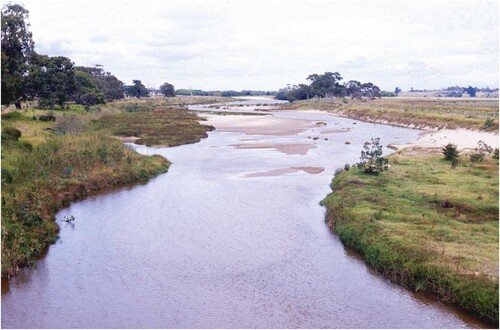
I first encountered Paul in 1989, in Buchan, Victoria at a meeting of the Australia and New Zealand Geomorphology Group, when I was completing my PhD on braided river processes. In the first few days of the conference, speakers presented their papers and as they responded to questions from the audience the response, more often than not, was ‘ … I’m not quite sure of that, let’s wait until Paul gets here’ or ‘Paul’s getting here on Wednesday, so we’ll ask him then’. Paul was en route from Sydney to a new job in Melbourne at the time, and so arrived mid-week and gave his own talk, and suddenly the questions asked in the first part of the week started to be answered. What Paul was doing was addressing the interactions between the specific landscape features that were being discussed (see Figure 1) and fundamental processes at scales ranging from sub-continental to local and from millions of years to hydrological events. He was linking process to form, but at appropriate timescales and with an awareness of what was, and was not, important to consider at the specific scales at which different presenters were operating. Many of the questions that had arisen earlier in the week were, of course, specific to individual studies, each of which provided new and informative data, but not always the conceptual frameworks within which to answer the initial research questions.

Figure 1. A sand-bed river in Victoria, Australia with floodplain and in-channel sediments influenced by post-European settlement erosion (see Portenga et al., 2016). I forget the precise location, but the image is memorable as the photograph was taken on the day when I first met Paul Bishop.

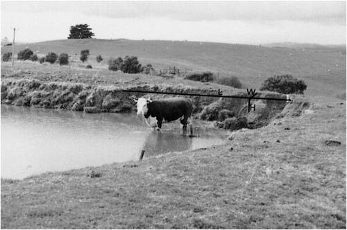
A few years later, Paul arrived in Glasgow soon after the publication of a paper urging caution in interpreting erosion measurements from small farm dams, including the figure reproduced here (Lloyd et al., 1998; see Figure 2). The importance of the figure is obviously not to show the geomorphological community what a cow looks like, but to encourage critical thought about how the cow interacts with the landscape and so influences the results of any measurements made in the dam lake. A sedimentation rate determined from the accumulation of sediment in the dam lake (in the image behind the cow) may be thought to be representative of the average erosion rate in the catchment, but what may actually be measured is how much erosion of the banks of the lake has been caused by the livestock. Hence, erosion rates measured from the dam sediments are likely to be overestimates of catchment erosion. There is a general message here that Paul emphasised to his students and colleagues: that when you make any measurements, you know precisely what you are measuring; and, when you take samples, you know precisely where to take samples to answer the questions that you wish to answer. Like all good advice, this sounds simple but is easy to forget or ignore.

Figure 2. ‘Livestock standing in a small farm dam’ (start of original caption from Lloyd et al., 1998).

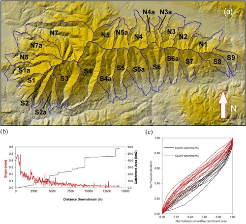
As many new measurement techniques have been developed over recent decades, the tendency to hurry to collect some samples and get some data remains, from which researchers try inductively to interpret that data without due attention to the details of the time, place and method of data collection. Paul took a consistently different approach. He was always deductive, based on consistent hypotheses and expectations, that were then to be tested critically against the data. The previous example illustrates the risks of measuring without careful a priori planning; without a careful sampling design, measurements may record the frequency of livestock movements up and down the bank, whereas the researcher may believe that they have measured catchment-averaged erosion rates and, therefore, may arrive at incorrect conclusions. The careful linkage of process to form coupled with deductive interpretation is what characterises Paul’s contributions to geomorphology. In the following sections, some examples are presented to demonstrate in more detail how this approach enabled Paul to make such profound and lasting contributions. Once in Glasgow, Paul formed a formidable collaboration with Brian Bluck (Williams, 2015) that included a series of research projects in the Sierra Nevada, Spain. The geomorphological research activity commenced with some simple observations of landscape and river morphology (Figure 3), from which a range of studies were developed, as described below.

Figure 3. (a) Catchments of the Sierra Nevada, Spain. Catchments labelled N drain northwards from the range, and those labelled S drain south towards the Mediterranean Sea. (b) River slope (red/lighter line) determined from GTOPO30 Digital Elevation Model and catchment area, for the Picena River (catchment S6). Note abrupt increases in catchment area at tributary junctions. (c) Normalised long profiles for the north (red/lighter) and south (black/darker) draining rivers. Unpublished data from John Jansen.

Revisiting river long profiles at multiple scales

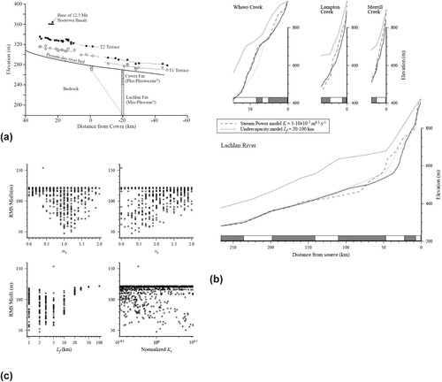
The Sierra Nevada work commenced in the late 1990s. Of course, Paul had been thinking about these issues for some time beforehand. Having mapped river terraces and the present-day riverbed in the Upper Lachlan catchment (Bishop et al., 1985; Bishop & Brown, 1992), Paul was not satisfied with speculating how these ancient and modern long profiles may have developed. As bedrock incision is driven by a combination of erosional processes, Paul deduced how different processes may result in different equilibrium river profiles. Having become aware of how early computer simulations of landscape evolution were able to predict long profile shape, Paul and Peter van der Beek undertook a pioneering modelling study to ‘test … quantitative fluvial incision models’, as the title of their paper puts it (van der Beek & Bishop, 2003). This paper is one of the first to consider how we can build fundamental sediment transport processes into a long-term model, simulate the development of river long profiles, and so bridge at least some of the gap between turbulence and tectonics noted in the introduction. Through this work, they asked questions such as: does it matter how in our modelling we drive sedimentary process? And, does it matter whether we have a simple model based on stream power or a more complicated one based on sediment supply and transport?

van der Beek and Bishop (2003) modelled the Upper Lachlan system under a range of assumptions and conditions (see Figure 4), and used Monte Carlo simulations to try to constrain the models better. Their conclusion is that, for the transport-limited stream power model and the nonlinear capacity and tools models, the optimal parameter combinations appear to have no physical significance, whereas for some models the best-fit parameter combinations are such that these models tend to mimic other models. That conclusion encapsulates Paul’s approach to these multi-parameter complex situations, in that he was not looking for the answer, but rather looking to constrain the range of possible answers to guide the next stage of the investigation. At that time, research into bedrock river incision was still developing, and their goal was to rule out the implausible and to work out where similar results may emerge for different parameter combinations, so as to guide where next to take the research. As such, this echoes Beven’s approach to catchment hydrological modelling (Beven, 2018; Beven & Lane, 2022), although the availability of data for model parameterisation and validation is very different in the two cases (see also Codilean et al., 2006).

Figure 4. Field data and model results from van der Beek and Bishop (2003). (a) Long profiles of the present-day Lachlan River, Australia and fluvial terraces, showing locations of the 12.5 Ma Boorowa basalt and alluvial fill at the bedrock-alluvial transition. (b) Modern river profiles for the Lachlan River and three tributary creeks predicted by two incision models, each of which includes variable lithologies shown in the boxes below each profile. Grey shading shows the Adaminaby Group metamorphics and white is the Wyangala Granite. (c) Results of Monte Carlo sampling of the parameter space for one of the models tested by van der Beek and Bishop (2003), the tools model. Plots show root mean square (RMS) of model misfit against four model parameters (m_t, n_t are exponents and normalised K_t is a constant in a transport-limited fluvial incision law, and L_f is a characteristic length scale for incision).

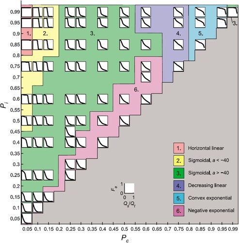
A significant body of research has followed on from van der Beek and Bishop’s (2003) starting point. As an example, building on many discussions with Paul regarding the links between grain-scale processes and long-term landscape response, Rebecca Hodge and I began to consider what might be revealed if we consider the implications of sediment transport processes (see Figure 5). In this case, clusters of sedimentary material are important because they protect the riverbed from erosion, reducing the rate of erosion occurring, and prior literature (e.g. Sklar & Dietrich, 2004) had suggested a simple form to this relationship. By modelling grain entrainment and clustering in multi-parameter space, we demonstrated that the relationship between bed erosion rate and sediment supply can take a range of shapes, depending on the combination of the probabilities of a grain moving and of becoming trapped in a cluster of bed material.

Figure 5. Relationships between sediment cover (F_e) and relative sediment supply (Q_s/Q_t, where Q_s is sediment supply and Q_t is the capacity sediment transport rate in the channel). A range of different forms of this relationship (colour coded and groups 1–6 in the legend) are found for combinations of the probabilities of entrainment of isolated grains (P_i) and cluster grains (P_c). Reproduced from Hodge and Hoey (2012).

This example shows Paul’s influence as he led us all to think about linkages between scales. Martin Williams (2023, this issue) tells us about this concern in relation to Paul’s early work on the Lachlan, and we can see how these principles then feed through into analysing the development of river long profiles. Moreover, through the work of several of our postgraduate students, we were able to start to think about these relationships between different scales. By way of illustration (see Figure 6), Jong Yeon Kim, one of our students at Glasgow, used a multi-scale approach to investigate the controls over long profile development in the River Etive, western Scotland (Kim, 2004). The long profile of the Etive shows a gradual reduction in gradient towards base level, but with some steep reaches. The steep reaches (shown in Figure 6) include waterfalls, which might be identified as knickpoints, only some of which have a clear lithological control. The knickzones contain bedforms of different types and there are strath terraces that record evidence of ancient long profiles prior to incision to the modern river bed level. These field observations led to asking questions about the micro-scale processes that are responsible for producing the long profile. To address this matter, Kim carried out some of the first laboratory tests of in situ river bed erosion, in which we put bedrock plates into a tumbling mill with sediment grains from the River Etive to generate impacts. The plates show erosion processes at the micro-scale (shown in Figure 6), down to showing differential weathering of feldspar and quartz grains under these impacts. The research challenge here was to determine how this river long profile had developed over post-glacial timescales through an ongoing combination of small-scale processes. Critically, Paul’s approach was never to be satisfied with generalisations, and he constantly questioned what exactly do we mean by abrasion, how does it operate, and how does it work at the grain scale? Once again, it is the link between scales that was crucial to some of the understanding that we derived from combining these laboratory experiments with numerical simulations and field observations.

Figure 6. Bedrock river long profiles and knickpoints at different scales. (a)-(d) (Kim, 2004) show knickpoints on the River Etive, Scotland, including sculpted bedforms (b) and incision below a strath terrace (d). (e) is part of the long profile of the River Etive, showing exposed bedrock (grey shading), alluvial cover (thick grey line) and strath terraces (dashed line). ¹⁰Be exposure ages of the strath terrace are plotted on the right y-axis. From Jansen et al. (2011). (f) SEM images (Kim, 2004) of bedrock plates from the River Etive following abrasion tests in a tumbling mill. Number on the upper image indicate different minerals (1 – feldspar; 2 – quartz). Arrows show impact marks from clasts in the tumbling mill. (g) Scaling of knickpoint retreat with catchment area for small streams along the east cost of Scotland (from Bishop et al., 2005).

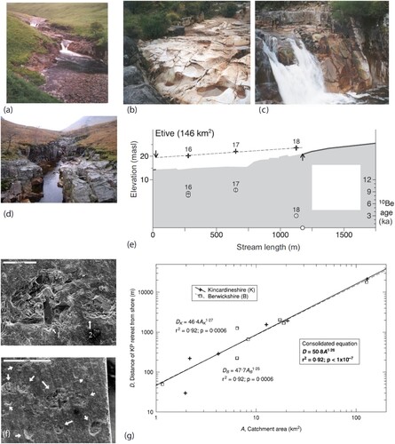
As Paul’s primary research interest was in the long-term evolution of landscapes, the logical next step to take when investigating knickpoint behaviour was to consider the scaling between knickpoint retreat rates and catchment size (Figure 6; Bishop et al., 2005). These results, later corroborated by data from elsewhere in Scotland (Castillo et al., 2013) showed that catchment area, and hence the erosive power of the rivers, was the primary control over post-glacial knickpoint retreat rates. This simple conclusion is very powerful in guiding interpretation of the development of transient landscapes.

Back to the Sierra Nevada: measuring the spatial variability of erosion to comprehend long-term landscape evolution

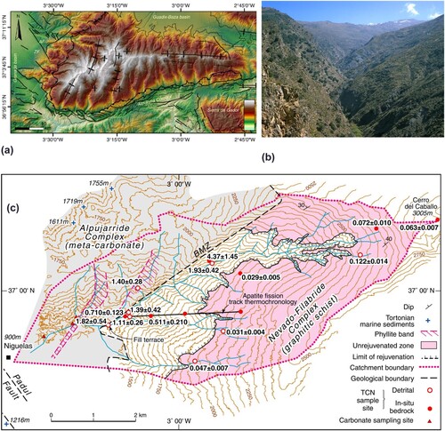
A further innovation that Paul initiated was to use cosmogenic isotopes to measure rates of in-channel processes, and the links between these and catchment-wide hillslope processes. Two PhD studies illustrate Paul’s approach here, again with multiple scales of analysis and thorough determination of process-form interactions. Liam Reinhardt worked in the Sierra Nevada, looking at the relationship between the catchment-wide erosion rates that can be measured from the river sediment rates and the erosion rates that we see on the hillslopes. The Sierra Nevada has a distinctive morphology that can be identified visually (see Figure 7) where the upper hillslopes appear to be at lower angles than many of the lower slopes, implying that the catchment is being incised in response to a base level change. The question is what can erosion rate measurements tell us about this apparent incision? In summary, Reinhardt’s sampling strategy was designed to test the hypothesis that a migrating wave of erosion is moving up this catchment. The upper catchment erosion rates on the hillslopes are around 0.05–0.10 mm year⁻¹, which are surprisingly low for the headwaters of an active orogen. However, in the lower catchment erosion rates are around 0.70–1.80 mm year⁻¹, an order of magnitude higher than in the upper part, and much more typical of orogenic erosion rates.

Figure 7. Erosion of the Sierra Nevada, Spain. (a) digital elevation model (Pérez-Peña et al., 2010) showing the overall E-W orientation of the mountain range, with the highest elevation terrain towards the western end. The Rio Torrente catchment is on the SW margin of the range. (b) View of the upper part of the Rio Torrente catchment, looking NE towards the peak of Cerro de Caballo (3005m). (c) Topographic map of the Rio Torrent catchment, showing in site and detrital ¹⁰Be erosion rates (Reinhardt et al., 2007a).

This study applied what were, at the time, very new geochronology techniques in a conceptually informed manner. At this time, in the late 1990s before the Scottish Universities Environmental Research Centre (SUERC: see Philo & Briggs, 2023, this issue) had the capability to make measurements of cosmogenic beryllium, we made the measurements at the Australian National University (ANU) with Keith Fifield. The careful collection and preparation of the samples allowed us to demonstrate that this new technique could provide reliable data from this very rapidly eroding terrain, and so added to the rationale for a cosmogenic isotope facility at SUERC. The data then allowed us to answer some fundamental questions about what is driving landscape evolution in this active orogen. Reinhardt et al., (2007a) demonstrated the role of base-level controlled knickpoint retreat, accelerated erosion downstream from the knickpoints, and was one of the first studies to quantify the long-standing geomorphological concept of landscape rejuvenation (Bishop, 2007).

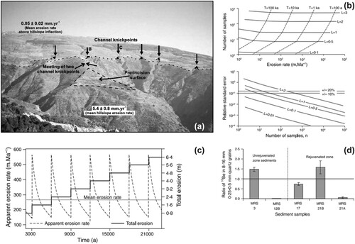
But, of course, Paul would not let us stop there. The slopes in the upper part of the rapidly eroding zone of the Sierra Nevada landscape are dominated by landslides, and so Paul’s challenge was to find a way to assess the contribution of landslides to the overall erosion pattern. Conceptually, a model was developed that demonstrated expectations of what would happen to the erosion rate depending on the landslide frequency. Note that at depths greater than about 3 metres there is negligible cosmogenic isotope accumulation, so if landslides are more than 3 metres deep they access rock that has zero concentration, but shallower landslides do mobilise material with inherited isotope concentrations. Knowing this fact allows us to calculate erosion rates as a function of landslide depth and landslide frequency (see Figure 8), from which we were able to interrogate the underlying processes. This was done by considering how different grain sizes might assist in identifying processes. So, we made cosmogenic isotope measurements in the 8–16 millimetre fraction – representing coarse landslide fragments – and in the sand fraction, and examined how the ratio of cosmogenic ¹⁰Be concentration between these two fractions varied across the landscape. The results corroborated the visual interpretation of the landscape, namely that landsliding was the dominant erosional mechanism in the steeper parts of the catchment whereas slower processes, mainly soil creep, dominated in the lower gradient areas. For the Sierra Nevada, therefore, we arrive at an understanding that there are two elements of the landscape that are in dynamic equilibrium: that of the upper catchment, which has low relief and shallow slopes dominated by soil creep; and, that of the lower catchment, which has threshold slopes of about 35 degrees and is dominated by river incision. Between these landscapes is a boundary marked by a zone of transience as the incision migrates up catchment.

Figure 8. (a) View of the Rio Torrente catchment showing the contrast between rapid erosion below the knickpoints and slow erosion on the lower gradient upper catchment terrain (Reinhardt et al., 2007a). (b) Estimates of the number of erosion rate estimates (upper plot) required to generate standard error = 0.2 mean erosion rate as a function of erosion rate, spalling thickness (L) and detachment recurrence interval (T). Lower plot shows the relative standard error as a function of the number of samples (Reinhardt et al., 2007b). (c) Modelled measured (dashed lines) and mean (solid grey line) erosion rates for a 0.8m bedrock chip removed every 3000 years (Reinhardt et al., 2007b). (d) Relative ¹⁰Be concentrations for 8-16mm and 0.25-0.5mm size fractions in detrital sediment samples from the Rio Torrente (Reinhardt et al., 2007b).

The message from this example is not about applying new techniques per se, but rather is about using these measurement techniques in an informed way when combining the interpretation of the data with modelling what you would expect (predicted outcomes) to guide interpretation and understanding. This is in many ways the classic Bishop approach: innovative technical work combined with geomorphic theory and deductive hypotheses to address fundamental research questions. The innovation is crucial, for exciting colleagues and students and, critically, funding bodies.

The world in a grain of sand?

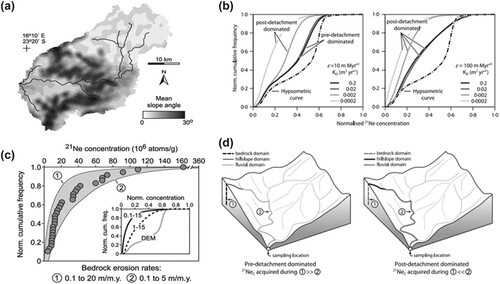
One of the most exciting developments in geomorphology has been the extension of measurement technologies to single grains (Bulur et al., 2002; Codilean et al., 2008, 2009). Single-grain analysis is not possible in the Sierra Nevada because the erosion rates are too rapid to allow measurable cosmogenic isotope concentrations to accumulate, but in certain other parts of the world this does become a feasible approach. Paul encouraged Tibi Codilean, another postgraduate student, to find a location where we could test the effectiveness of single-grain, stable cosmogenic isotope measurements. Codilean identified Namibia as an environment where we could once again analyse landscape evolution under steady-state and transient conditions, but at a very different timescale to the Sierra Nevada. The Namibian landscape is generally low gradient with isolated hills (see Figure 9), this time with steep slopes in the upper catchment and very flat slopes in the lower catchment. The measurements in this case are of stable ²¹Ne, which was a novel cosmogenic technique at the time, and remains underused. Modelling took place in a GIS framework to simulate what expected frequency distributions of isotope concentrations in grains moving through this landscape. The results (shown in Figure 9) were compared with multiple simulations to determine the influence of certain key parameters, specifically those relating to climate, the frequency of grain movement and erosion rates in the rivers and on the hillslopes. This modelling allowed assessment of the extent to which measured cosmogenic isotope concentrations in individual grains are acquired while the grains are still attached to the bedrock, after they have left the bedrock and are moving over the hillside slowly, or after they have entered the river channel and are moving much more quickly. The approach is to be patient and to analyse the different parts of the process carefully, so that we avoid lumping things together, trying forensically to ‘fingerprint’ the origins of these isotopic concentrations in the grains.

Figure 9. (a) Spatial distribution of mean slope in the upper Gaub River catchment (Namibia) (Codilean et al., 2008). (b) Normalised ²¹Ne concentration distributions for different assumptions regarding the timing of erosion (Codliean et al., 2009). (c) Cumulative frequency distribution from 32 measurements of ²¹Ne in individual clasts in Gaub River sediments. Inset shows simulated cumulative frequency distributions of ²¹Ne for two different assumptions of the dependence of erosion rate on catchment slope, and the hypsometry of the catchment (DEM) (Codliean et al., 2008).

While the Namibian and Sierra Nevada cases appear different, there are many similarities in how the data are interpreted. In both cases, the relationship between geomorphic processes and landscape-scale features has been identified, and the cosmogenic isotope measurements validate hypotheses concerning the development of dynamic equilibria over appropriate timescales. As with Kim’s work on the River Etive, and other studies that Paul has initiated (e.g. Castillo et al., 2013; Jansen et al., 2010; Whitbread et al., 2015), detailed measurements and deductive, testable hypotheses allow reconciliation of features and processes across spatial and temporal scales. For a geomorphologist to ‘observe complexity and see simplicity’ (cf. Stark, 2000) is a career-defining capability that Paul undoubtedly possessed and that he tried, as the previous examples illustrate, to pass on to his students and colleagues.

Conclusion: Paul Bishop’s geomorphology

The stripes shown in Figure 10, are becoming almost ubiquitous in our daily lives, adorning mugs, ties, book covers, newspapers and, of course, appearing in scientific discourse (Dixon, 2023). They offer a powerful representation of how the planet's climatic-temperature regime has oscillated but with such an obvious warming trend over recent years. They also provide an appropriate metaphor to describe developments in the discipline of geomorphology, and in physical geography and earth sciences more generally, over recent decades. In Figure 10, Paul’s career is mapped on to the stripes. The first three letters that came up when planning this exercise were B, F and G: the ‘Big Friendly Giant’ (BFG) (see Philo & Briggs, 2023, this issue). Indeed, Paul was born (B) during a ‘cold period’; he published his first major paper (F) to coincide with a little warm stripe in 1980, although I now realise that there was some published work from slightly earlier (see Williams, 2023, this issue); and he moved to Glasgow (G) at the time when the ‘reddening’ was taking over. As in any long career, a wide range of measurement and modelling techniques became available at different stages of Paul’s career. When he started in 1980, apatite-fission track analysis was relatively new, apatite uranium, thorium and helium analysis had not been developed as a tool for geochronology, cosmogenic isotopes were a largely theoretical concept (Lal, 1991), luminescence was in its infancy, and even techniques that were widely used, such as radiocarbon dating, have changed dramatically since then. As is the case for all of us as we go through our careers, things change. A critical skill is to adapt to these changes, not seeing them as threats but as opportunities. Paul was perhaps particularly distinctive in how he constantly used such technical developments as opportunities throughout his career, never rushing towards the latest fashion but always working with new methods in a conceptually-informed manner, continually asking how the innovations could help him in his quest to better understand landscape.

Figure 10. Summarising Paul’s career in context. Challenges are generalised (see Church, 2010). Photograph is of Paul (with hat) with Tim Dempster in the Sierra Nevada, Spain. Climate stripes from Hawkins (2018) show the period 1850–2020. B – birth of Paul Bishop; F – date of his first paper as lead author (Bishop, 1980); G – Paul moves to University of Glasgow.

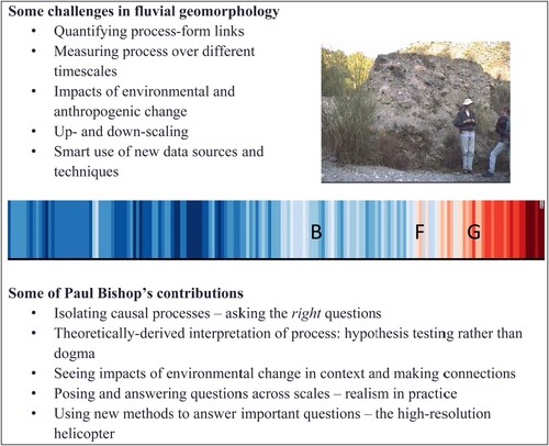
In the top left of Figure 10 I have summarised in very few words, which do not do justice to the complexity of the arguments here, some of the challenges that fluvial geomorphologists have faced, and continue to face, many of which have been of concern for decades. In the lower part of the graphic, not mapped one-to-one on to these challenges, are some comments and thoughts about Paul’s contributions. The isolating of causal processes, and asking the right sorts of questions, is something that Paul has done throughout his career, making sure that we think in advance ‘what is it that we really want to know?’ It was always vital for Paul that we are not faced with the problem of post hoc rationalisation of data collected for its own sake, but that we always collect data with a goal or series of goals in mind. His emphasis was always on prior deductive thinking, thinking that was long, hard, deep and smart. Paul was a strong advocate of hypothesis-testing, trying to move beyond dogma and to ensure that we are, as far as possible, objective. Paul knew the challenges of objectivity, but insisted on standing back from the problem at hand, asking the right questions, and making meaningful connections. He was always a brilliant thinker in this regard, making connections between the apparently unconnected, and asking ‘what do you think of that?’ of whoever he was interacting with at that moment.

This stance before the world might be characterised as ‘realism in practice’, and a paper that Paul, Rob Ferguson and I wrote two decades ago (Hoey et al., 2003) sought to deploy a realist philosophical approach to explain how a lot of geomorphology actually does work in practice: in a realist approach, examination of related phenomena at the same scale, combined with consideration of the same phenomena at and across different scales, enables insights from this intersection of scales to significantly advance geomorphologists’ understanding. Paul truly was very good at doing that: whether or not he would have agreed that it was realism in a philosophical sense or not is less important than the fact that it was his way of operating.

Paul’s approach helped him in always thinking about how new methods could help to answer what are actually important questions. We are often told to examine complex problems by taking ‘a helicopter view’, where you take yourself high above what you are looking at, what issue or concern needs to be addressed, and look down from above. Often from that height the issue in question is almost lost from view, its details and specificities no longer detectable, but what Paul was especially great at doing was adopting a high-resolution helicopter view. His binoculars were obviously quite sharp in focus and powerful because he could occupy his virtual helicopter and continue to ask the detailed, precise and crucial question that unlocked the next level of understanding. This precision and focus represent a deceptively great contribution that was, is, and will continue to be, the mark of Paul Bishop’s geomorphology.

Acknowledgements

Many thanks to all of the former undergraduate and PhD students, post-doctoral researchers and colleagues of Paul’s and mine who have helped with the research and ideas discussed herein. The list is too long to mention, and there would always be the risk of omitting someone, but your contributions to delivering Paul’s legacy are each essential. The audience at the symposium to honour Paul provided valuable insight and feedback. Particular thanks to Chris Philo for transcribing my words on that occasion and insightful suggestions on the manuscript, and to Martin Hurst and Daniel Peifer for many helpful suggestions and clarifications. Specific thanks are due to the following people for their generous permissions to reproduce materials (maps, graphs, images, etc.) in the composite figures created specially for this article: Ivars Reinfelds (Figure 2); Peter van der Beek (Figure 4); Jong Yeon Kim (Figure 6); Liam Reinhardt (Figures 7 and 8); and Tibi Codilean (Figure 9).

Disclosure statement

No potential conflict of interest was reported by the author(s).

References

- Beven, K. J. (2018). On hypothesis testing in hydrology: Why falsification of models is still a really good idea. WIRES Water, 5(3), e1278. https://doi.org/10.1002/wat2.1278
- Beven, K. J., & Lane, S. N. (2022). On (in)validating environmental models. 1. Principles for formulating a Turing-like Test for determining when a model is fit-for purpose. Hydrological Processes, 36(10), e14704. https://doi.org/10.1002/hyp.14704
- Bishop, P. (1980). Popper's principle of falsifiability and the irrefutability of the Davisian cycle. The Professional Geographer, 32(3), 310–315. https://doi.org/10.1111/j.0033-0124.1980.00310.x
- Bishop, P. (2007). Long-term landscape evolution: Linking tectonics and surface processes. Earth Surface Processes and Landforms, 32(3), 329–365. https://doi.org/10.1002/esp.1493
- Bishop, P., & Brown, R. (1992). Denudational isostatic rebound of intraplate highlands: The Lachlan river valley, Australia. Earth Surface Processes and Landforms, 17(4), 345–360. https://doi.org/10.1002/esp.3290170405
- Bishop, P., Hoey, T. B., Jansen, J. D., & Lexartza Artza, I. (2005). Knickpoint recession rate and catchment area: The case of uplifted rivers in eastern Scotland. Earth Surface Processes and Landforms, 30(6), 767–778. https://doi.org/10.1002/esp.1191
- Bishop, P., Young, R. W., & McDougall, I. (1985). Stream profile change and longterm landscape evolution: Early miocene and modern rivers of the east Australian highland crest, central New South Wales, Australia. The Journal of Geology, 93(4), 455–474. https://doi.org/10.1086/628966
- Bulur, E., Duller, G. A. T., Solongo, S., Bøtter-Jensen, L., & Murray, A. S. (2002). LM-OSL from single grains of quartz: A preliminary study. Radiation Measurements, 35(1), 79–85. https://doi.org/10.1016/S1350-4487(01)00256-6
- Castillo, M., Jansen, J., & Bishop, P. (2013). Knickpoint retreat and transient bedrock channel morphology triggered by base-level fall in small bedrock river catchments: The case of the Isle of Jura, Scotland. Geomorphology, 180-181, 1–9. https://doi.org/10.1016/j.geomorph.2012.08.023
- Church, M. (1996). Space, time and the mountain - how do we order what we see? In B. L. Rhoads & C. E. Thorn (Eds.), The scientific nature of geomorphology (pp. 147–170).
- Church, M. (2010). The trajectory of geomorphology. Progress in Physical Geography: Earth and Environment, 34(3), 265–286. https://doi.org/10.1177/0309133310363992
- Codilean, A. T., Bishop, P., & Hoey, T. B. (2006). Surface process models and the links between tectonics and topography. Progress in Physical Geography: Earth and Environment, 30(3), 307–333. https://doi.org/10.1191/0309133306pp480ra
- Codilean, A. T., Bishop, P., Hoey, T. B., Stuart, F. M., & Fabel, D. (2009). Cosmogenic 21Ne analysis of individual detrital grains: Opportunities and limitations. Earth Surface Processes and Landforms, 35(1), 16–27. https://doi.org/10.1002/esp.1815
- Codilean, A. T., Bishop, P., Stuart, F. M., Hoey, T. B., Fabel, D., & Freeman, S. P. H. T. (2008). Single-grain cosmogenic 21Ne concentrations in fluvial sediments reveal spatially variable erosion rates. Geology, 36(2), 159–162. https://doi.org/10.1130/G24360A.135
- Dixon, D. (2023). In the breach: Feeling the heat of climate change. Scottish Geographical Journal, 139(1-2), 103–114. https://doi.org/10.1080/14702541.2022.2157867
- Hawkins, E. (2018). 2018 visualisation update. https://www.climate-lab-book.ac.uk/2018/2018-visualisation-update/.
- Hodge, R. A., & Hoey, T. B. (2012). Upscaling from grain-scale processes to alluviation in bedrock channels using a cellular automaton model. Journal of Geophysical Research: Earth Surface, 117, F01017. https://doi.org/10.1029/2011JF002145
- Hoey, T. B., Bishop, P., & Ferguson, R. I. (2003). Testing numerical models in geomorphology: How can we ensure critical use of model predictions? Chapter 17. In P. Wilcock & R. Iverson (Eds.), Prediction in geomorphology (vol. 135, pp. 241–256). AGU Geophysical Monograph. https://doi.org/10.1029/135GM017
- Hutton, J. (1795). Theory of the Earth: with proofs and illustrations. London and Edinburgh: Cadell, Junior and Davies; William Creech.
- Jansen, J. D., Codilean, A. T., Bishop, P., & Hoey, T. B. (2010). Scale dependence of lithological control on topography: Bedrock channel geometry and catchment morphometry in western Scotland. The Journal of Geology, 118(3), 223–246. https://doi.org/10.1086/651273
- Jansen, J. D., Fabel, D., Bishop, P., Xu, S., Schnabel, C., & Codilean, A. T. (2011). Does decreasing paraglacial sediment supply slow knickpoint retreat? Geology, 39(6), 543–546. https://doi.org/10.1130/G32018.1
- Kim, J.-Y. (2004). Controls over bedrock channel incision. Unpublished PhD thesis. University of Glasgow.
- Lal, D. (1991). Cosmic-ray labeling of erosion surfaces: In situ nuclide production rates and erosion models. Earth and Planetary Science Letters, 104(2-4), 424–439.
- Leeder, M. (2011). Sedimentology and sedimentary basins: From turbulence to tectonics. Wiley-Blackwell.
- Lloyd, S. D., Bishop, P., & Reinfelds, I. (1998). Shoreline erosion: A cautionary note in using small farm dams to determine catchment erosion rates. Earth Surface Processes and Landforms, 23(10), 905–912. https://doi.org/10.1002/(SICI)1096-9837(199810)23:10<905::AID-ESP910>3.0.CO;2-E
- Pérez-Peña, J. V., Azor, A., Azañón, J. M., & Keller, E. A. (2010). Active tectonics in the Sierra Nevada (Betic Cordillera, SE Spain): insights from geomorphic indexes and drainage pattern analysis. Geomorphology, 119(1-2), 74–87. https://doi.org/10.1016/j.geomorph.2010.02.020
- Philo, C., & Briggs, J. (2023). Paul Bishop: Recalling an academic life. Scottish Geographical Journal, this issue.
- Portenga, E. W., Westaway, K. E., & Bishop, P. (2016). Timing of post-European settlement alluvium deposition in SE Australia: A legacy of European land-use in the Goulburn plains. The Holocene, 26(9), 1472–1485. https://doi.org/10.1177/0959683616640047
- Reinhardt, L. J., Bishop, P., Hoey, T. B., Dempster, T. J., & Sanderson, D. C. W. (2007a). Quantification of the transient response to base-level fall in a small mountain catchment: Sierra Nevada, southern Spain. Journal of Geophysical Research, 112(F3), F03S–F005. https://doi.org/10.1029/2006JF000524
- Reinhardt, L. J., Hoey, T. B., Barrows, T. T., Dempster, T. J., Bishop, P., & Fifield, L. K. (2007b). Interpreting erosion rates from cosmogenic radionuclide concentrations measured in rapidly eroding terrain. Earth Surface Processes and Landforms, https://doi.org/10.1002/esp.1415
- Schumm, S. A., & Lichty, R. W. (1965). Time, space and causality in geomorphology. American Journal of Science, 263(2), 110–119. https://doi.org/10.2475/ajs.263.2.110
- Sklar, L. S., & Dietrich, W. E. (2004). A mechanistic model for river incision into bedrock by saltating bed load. Water Resources Research, 40(6), W06301. https://doi.org/10.1029/2003WR002496
- Stark, J. (2000). Observing complexity, seeing simplicity. Philosophical Transactions of the Royal Society of London. Series A: Mathematical, Physical and Engineering Sciences, 358(1765), 41–61. https://doi.org/10.1098/rsta.2000.0518
- van der Beek, P., & Bishop, P. (2003). Cenozoic river profile development in the Upper Lachlan catchment (SE Australia) as a test of quantitative fluvial incision models. Journal of Geophysical Research – Solid Earth, 108(B6), https://doi.org/10.1029/2002JB002125.
- Whitbread, K., Jansen, J., Bishop, P., & Attal, M. (2015). Substrate, sediment, and slope controls on bedrock channel geometry in postglacial streams. Journal of Geophysical Research: Earth Surface, 120(5), 779–798. https://doi.org/10.1002/2014JF003295
- Williams, B. (2015). Brian John Bluck 1935-2015. The Geological Society. https://www.geolsoc.org.uk/About/History/Obituaries-2001-onwards/Obituaries-2015/Brian-John-Bluck–1935–2015.
- Williams, M. (2023). Paul Bishop: The early years in Australia and Ethiopia. Scottish Geographical Journal. https://doi.org/10.1080/14702541.2023.2233943